2 Asymptotic expansion of expectation of Wiener functionals
We prepare notation and definitions on Malliavin calculus on an abstract Wiener space. For the details, see Watanabe (1984) [25 ] , Ikeda and Watanabe (1989) [9 ] , Üstünel (1995) [23 ] , Malliavin (1997) [13 ] , Üstünel and Zakai (2000) [24 ] , Nualart (2006) [16 ] and Matsumoto and Taniguchi (2016) [15 ] .
Let ( 𝒲 , ℋ , μ ) 𝒲 ℋ 𝜇 \displaystyle({\cal W},{\cal H},\mu) 𝒲 𝒲 \displaystyle{\cal W} ℋ ℋ \displaystyle{\cal H} 𝒲 𝒲 \displaystyle{\cal W} j : ℋ → 𝒲 : 𝑗 → ℋ 𝒲 \displaystyle j:{\cal H}\to{\cal W} 𝒲 ′ superscript 𝒲 ′ \displaystyle{\cal W}^{\prime} ℋ ′ superscript ℋ ′ \displaystyle{\cal H}^{\prime} 𝒲 𝒲 \displaystyle{\cal W} ℋ ℋ \displaystyle{\cal H} 𝒲 ′ ↪ j ∗ ℋ ′ = ℋ ↪ 𝑗 𝒲 superscript 𝒲 ′ superscript 𝑗 ∗ ↪ superscript ℋ ′ ℋ 𝑗 ↪ 𝒲 \displaystyle{\cal W}^{\prime}\overset{j^{\ast}}{\hookrightarrow}{\cal H}^{\prime}={\cal H}\overset{j}{\hookrightarrow}{\cal W} j ∗ superscript 𝑗 ∗ \displaystyle j^{\ast} j 𝑗 \displaystyle j μ 𝜇 \displaystyle\mu ( 𝒲 , ℬ ( 𝒲 ) ) 𝒲 ℬ 𝒲 \displaystyle({\cal W},\mathscr{B}(\cal W))
∫ 𝒲 e i 𝒲 ′ ⟨ l , ω ⟩ 𝒲 𝑑 μ ( ω ) = e − 1 2 ‖ j ∗ ( l ) ‖ ℋ 2 , for all l ∈ 𝒲 ′ . formulae-sequence subscript 𝒲 superscript 𝑒 subscript i superscript 𝒲 ′ subscript 𝑙 𝜔
𝒲 differential-d 𝜇 𝜔 superscript 𝑒 1 2 superscript subscript norm superscript 𝑗 ∗ 𝑙 ℋ 2 for all 𝑙 superscript 𝒲 ′ \displaystyle\displaystyle\int_{{\cal W}}e^{\mathrm{i}_{{\cal W}^{\prime}}\langle l,\omega\rangle_{{\cal W}}}d\mu(\omega)=e^{-\frac{1}{2}\|j^{\ast}(l)\|_{{\cal H}}^{2}},\ \ \mbox{for all}\ l\in{\cal W}^{\prime}. (2.1)
Hence { 𝒲 ′ ⟨ l , ⋅ ⟩ 𝒲 ; l ∈ 𝒲 ′ } \displaystyle\{_{{\cal W}^{\prime}}\langle l,\cdot\rangle_{{\cal W}};\ l\in{\cal W}^{\prime}\} ( 𝒲 , ℬ ( 𝒲 ) , μ ) 𝒲 ℬ 𝒲 𝜇 \displaystyle({\cal W},\mathscr{B}(\cal W),\mu) 0 0 \displaystyle 0 𝔼 [ 𝒲 ′ ⟨ l , ω ⟩ 𝒲 ⟨ l ′ , ω ⟩ 𝒲 𝒲 ′ ] = ⟨ j ∗ ( l ) , j ∗ ( l ′ ) ⟩ ℋ \displaystyle\mathbb{E}[_{{\cal W}^{\prime}}\langle l,\omega\rangle_{{\cal W}}\ {}_{{\cal W}^{\prime}}\langle l^{\prime},\omega\rangle_{{\cal W}}]=\langle j^{\ast}(l),j^{\ast}(l^{\prime})\rangle_{{\cal H}} l , l ′ ∈ 𝒲 ′ 𝑙 superscript 𝑙 ′
superscript 𝒲 ′ \displaystyle l,l^{\prime}\in{\cal W}^{\prime} j ∗ ( 𝒲 ′ ) ∋ j ∗ ( l ) ↦ 𝒲 ′ ⟨ l , ⋅ ⟩ 𝒲 ∈ L 2 ( 𝒲 ) contains superscript 𝑗 ∗ superscript 𝒲 ′ superscript 𝑗 ∗ 𝑙 subscript maps-to superscript 𝒲 ′ subscript 𝑙 ⋅
𝒲 superscript 𝐿 2 𝒲 \displaystyle j^{\ast}({\cal W}^{\prime})\ni j^{\ast}(l)\ \mapsto\ _{{\cal W}^{\prime}}\langle l,\cdot\rangle_{{\cal W}}\in L^{2}({\cal W}) I : ℋ → L 2 ( 𝒲 ) : 𝐼 → ℋ superscript 𝐿 2 𝒲 \displaystyle I:{\cal H}\to L^{2}({\cal W}) I ( h ) 𝐼 ℎ \displaystyle I(h) 0 0 \displaystyle 0 ‖ I ( h ) ‖ L 2 ( 𝒲 ) = ‖ h ‖ ℋ subscript norm 𝐼 ℎ superscript 𝐿 2 𝒲 subscript norm ℎ ℋ \displaystyle\|I(h)\|_{L^{2}({\cal W})}=\|h\|_{{\cal H}} j ∗ ( 𝒲 ) ⊂ ℋ superscript 𝑗 ∗ 𝒲 ℋ \displaystyle j^{\ast}({\cal W})\subset{\cal H}
Let 𝒮 ( 𝒲 ) = { F : 𝒲 → ℝ ; F = f ( I ( h 1 ) , … , I ( h n ) ) , n ∈ ℕ , f ∈ C b ∞ ( ℝ n ) , h 1 , … , h n ∈ ℋ } 𝒮 𝒲 conditional-set 𝐹 formulae-sequence → 𝒲 ℝ formulae-sequence 𝐹 𝑓 𝐼 subscript ℎ 1 … 𝐼 subscript ℎ 𝑛 formulae-sequence 𝑛 ℕ formulae-sequence 𝑓 superscript subscript 𝐶 𝑏 superscript ℝ 𝑛 subscript ℎ 1 …
subscript ℎ 𝑛 ℋ \displaystyle\mathscr{S}({\cal W})=\{F:{\cal W}\to\mathbb{R};\ F=f(I(h_{1}),\ldots,I(h_{n})),\ n\in\mathbb{N},\ f\in C_{b}^{\infty}(\mathbb{R}^{n}),h_{1},\ldots,h_{n}\in{\cal H}\} F = f ( I ( h 1 ) , … , I ( h n ) ) ∈ 𝒮 ( 𝒲 ) 𝐹 𝑓 𝐼 subscript ℎ 1 … 𝐼 subscript ℎ 𝑛 𝒮 𝒲 \displaystyle F=f(I(h_{1}),\ldots,I(h_{n}))\in\mathscr{S}({\cal W}) D F ∈ ℋ 𝐷 𝐹 ℋ \displaystyle DF\in{\cal H}
D F = ∑ i = 1 n ( ∂ i f ) ( I ( h 1 ) , … , I ( h n ) ) h i . 𝐷 𝐹 superscript subscript 𝑖 1 𝑛 subscript 𝑖 𝑓 𝐼 subscript ℎ 1 … 𝐼 subscript ℎ 𝑛 subscript ℎ 𝑖 \displaystyle\displaystyle DF=\sum_{i=1}^{n}(\partial_{i}f)(I(h_{1}),\ldots,I(h_{n}))h_{i}. (2.2)
The operator D 𝐷 \displaystyle D p > 1 𝑝 1 \displaystyle p>1 𝔻 1 , p = 𝒮 ( 𝒲 ) ¯ ∥ ⋅ ∥ 1 , p \displaystyle\mathbb{D}^{1,p}=\overline{\mathscr{S}({\cal W})}^{\|\cdot\|_{1,p}} ∥ ⋅ ∥ 1 , p \displaystyle\|\cdot\|_{1,p} ‖ F ‖ 1 , p = ‖ F ‖ ℒ p ( 𝒲 ) + ‖ D F ‖ ℒ p ( 𝒲 ; ℋ ) subscript norm 𝐹 1 𝑝
subscript norm 𝐹 superscript ℒ 𝑝 𝒲 subscript norm 𝐷 𝐹 superscript ℒ 𝑝 𝒲 ℋ
\displaystyle\|F\|_{1,p}=\|F\|_{{\cal L}^{p}({\cal W})}+\|DF\|_{{\cal L}^{p}({\cal W};{\cal H})} D k superscript 𝐷 𝑘 \displaystyle D^{k} 𝔻 k , p superscript 𝔻 𝑘 𝑝
\displaystyle\mathbb{D}^{k,p} 𝔻 ∞ = ∩ k ∈ ℕ , p > 1 𝔻 k , p superscript 𝔻 subscript formulae-sequence 𝑘 ℕ 𝑝 1 superscript 𝔻 𝑘 𝑝
\displaystyle\mathbb{D}^{\infty}=\cap_{k\in\mathbb{N},p>1}\mathbb{D}^{k,p}
Let Dom δ = { u ∈ L 2 ( 𝒲 ; ℋ ) ; ∃ C > 0 s.t. | 𝔼 [ ⟨ D F , u ⟩ ℋ ] | ≤ C ∥ F ∥ L 2 ( 𝒲 ) , ∀ F ∈ 𝔻 1 , 2 } \displaystyle\mathrm{Dom}\delta=\{u\in L^{2}({\cal W};{\cal H});\ \exists C>0\mbox{ s.t. }|\mathbb{E}[\langle DF,u\rangle_{{\cal H}}]|\leq C\|F\|_{L^{2}({\cal W})},\forall F\in\mathbb{D}^{1,2}\} u ∈ Dom δ 𝑢 Dom 𝛿 \displaystyle u\in\mathrm{Dom}\delta δ ( u ) ∈ L 2 ( 𝒲 ) 𝛿 𝑢 superscript 𝐿 2 𝒲 \displaystyle\delta(u)\in L^{2}({\cal W})
𝔼 [ ⟨ D F , u ⟩ ℋ ] = 𝔼 [ F δ ( u ) ] , 𝔼 delimited-[] subscript 𝐷 𝐹 𝑢
ℋ 𝔼 delimited-[] 𝐹 𝛿 𝑢 \displaystyle\displaystyle\mathbb{E}[\langle DF,u\rangle_{{\cal H}}]=\mathbb{E}[F\delta(u)], (2.3)
which is called the duality formula.
For a multi-index α = ( α 1 , … , α k ) 𝛼 subscript 𝛼 1 … subscript 𝛼 𝑘 \displaystyle\alpha=(\alpha_{1},\ldots,\alpha_{k}) | α | = ∑ i = 1 k α i = n 𝛼 superscript subscript 𝑖 1 𝑘 subscript 𝛼 𝑖 𝑛 \displaystyle|\alpha|=\textstyle{\sum_{i=1}^{k}}\alpha_{i}=n I n : ℋ ⊗ n → ℝ : subscript 𝐼 𝑛 → superscript ℋ tensor-product absent 𝑛 ℝ \displaystyle I_{n}:{\cal H}^{\otimes n}\to\mathbb{R}
I n ( h 1 ⊗ α 1 ⊗ ⋯ ⊗ h k ⊗ α k ) = α ! ∏ i = 1 k H α i ( δ ( h i ) ) , subscript 𝐼 𝑛 tensor-product superscript subscript ℎ 1 tensor-product absent subscript 𝛼 1 ⋯ superscript subscript ℎ 𝑘 tensor-product absent subscript 𝛼 𝑘 𝛼 superscript subscript product 𝑖 1 𝑘 subscript 𝐻 subscript 𝛼 𝑖 𝛿 subscript ℎ 𝑖 \displaystyle\displaystyle I_{n}(h_{1}^{\otimes\alpha_{1}}\otimes\cdots\otimes h_{k}^{\otimes\alpha_{k}})=\alpha!\prod_{i=1}^{k}H_{\alpha_{i}}(\delta(h_{i})), (2.4)
where α ! = ∏ i = 1 k α k ! 𝛼 superscript subscript product 𝑖 1 𝑘 subscript 𝛼 𝑘 \displaystyle\alpha!=\textstyle{\prod_{i=1}^{k}}\alpha_{k}! H ℓ ( ⋅ ) subscript 𝐻 ℓ ⋅ \displaystyle H_{\ell}(\cdot) ℓ ℓ \displaystyle\ell F ∈ 𝔻 ∞ , 2 𝐹 superscript 𝔻 2
\displaystyle F\in\mathbb{D}^{\infty,2}
F = 𝔼 [ F ] + ∑ p ≥ 1 1 p ! I p ( 𝔼 [ D p F ] ) . 𝐹 𝔼 delimited-[] 𝐹 subscript 𝑝 1 1 𝑝 subscript 𝐼 𝑝 𝔼 delimited-[] superscript 𝐷 𝑝 𝐹 \displaystyle\displaystyle F=\mathbb{E}[F]+\sum_{p\geq 1}\frac{1}{p!}I_{p}(\mathbb{E}[D^{p}F]). (2.5)
For F = ( F 1 , … , F e ) ∈ ( 𝔻 ∞ ) e 𝐹 superscript 𝐹 1 … superscript 𝐹 𝑒 superscript superscript 𝔻 𝑒 \displaystyle F=(F^{1},\ldots,F^{e})\in(\mathbb{D}^{\infty})^{e} σ F = [ σ i j F ] 1 ≤ i , j ≤ e superscript 𝜎 𝐹 subscript delimited-[] subscript superscript 𝜎 𝐹 𝑖 𝑗 formulae-sequence 1 𝑖 𝑗 𝑒 \displaystyle\sigma^{F}=[\sigma^{F}_{ij}]_{1\leq i,j\leq e}
σ i j F = ⟨ D F i , D F j ⟩ ℋ , 1 ≤ i , j ≤ e . formulae-sequence subscript superscript 𝜎 𝐹 𝑖 𝑗 subscript 𝐷 superscript 𝐹 𝑖 𝐷 superscript 𝐹 𝑗
ℋ formulae-sequence 1 𝑖 𝑗 𝑒 \displaystyle\displaystyle\sigma^{F}_{ij}=\langle DF^{i},DF^{j}\rangle_{{\cal H}},\ \ \ 1\leq i,j\leq e. (2.6)
We say F ∈ ( 𝔻 ∞ ) e 𝐹 superscript superscript 𝔻 𝑒 \displaystyle F\in(\mathbb{D}^{\infty})^{e} σ F superscript 𝜎 𝐹 \displaystyle\sigma^{F}
‖ det ( σ F ) − 1 ‖ ℒ p ( 𝒲 ) < ∞ , ∀ p > 1 . formulae-sequence subscript norm superscript superscript 𝜎 𝐹 1 superscript ℒ 𝑝 𝒲 for-all 𝑝 1 \displaystyle\displaystyle\|\det(\sigma^{F})^{-1}\|_{{\cal L}^{p}({\cal W})}<\infty,\ \ \ \forall p>1. (2.7)
Let 𝒮 ( ℝ e ) 𝒮 superscript ℝ 𝑒 \displaystyle\mathcal{S}(\mathbb{R}^{e}) ℝ ℝ \displaystyle\mathbb{R} ℝ e superscript ℝ 𝑒 \displaystyle\mathbb{R}^{e} F ∈ ( 𝔻 ∞ ) e 𝐹 superscript superscript 𝔻 𝑒 \displaystyle F\in(\mathbb{D}^{\infty})^{e} G ∈ 𝔻 ∞ 𝐺 superscript 𝔻 \displaystyle G\in\mathbb{D}^{\infty} f ∈ 𝒮 ( ℝ e ) 𝑓 𝒮 superscript ℝ 𝑒 \displaystyle f\in\mathcal{S}(\mathbb{R}^{e}) α ∈ { 1 , … , e } k 𝛼 superscript 1 … 𝑒 𝑘 \displaystyle\alpha\in\{1,\ldots,e\}^{k}
𝔼 [ ∂ α f ( F ) G ] = 𝔼 [ f ( F ) H α ( F , G ) ] , 𝔼 delimited-[] superscript 𝛼 𝑓 𝐹 𝐺 𝔼 delimited-[] 𝑓 𝐹 subscript 𝐻 𝛼 𝐹 𝐺 \displaystyle\displaystyle\mathbb{E}[\partial^{\alpha}f(F)G]=\mathbb{E}[f(F)H_{\alpha}(F,G)], (2.8)
where H α ( F , G ) subscript 𝐻 𝛼 𝐹 𝐺 \displaystyle H_{\alpha}(F,G) H α ( F , G ) = H ( α k ) ( F , H ( α 1 , … , α k − 1 ) ( F , G ) ) subscript 𝐻 𝛼 𝐹 𝐺 subscript 𝐻 subscript 𝛼 𝑘 𝐹 subscript 𝐻 subscript 𝛼 1 … subscript 𝛼 𝑘 1 𝐹 𝐺 \displaystyle H_{\alpha}(F,G)=H_{(\alpha_{k})}(F,H_{(\alpha_{1},\ldots,\alpha_{k-1})}(F,G))
H ( i ) ( F , G ) = ∑ j = 1 e δ ( γ i j F D F j G ) , i = 1 , … , e , formulae-sequence subscript 𝐻 𝑖 𝐹 𝐺 superscript subscript 𝑗 1 𝑒 𝛿 subscript superscript 𝛾 𝐹 𝑖 𝑗 𝐷 superscript 𝐹 𝑗 𝐺 𝑖 1 … 𝑒
\displaystyle\displaystyle H_{(i)}(F,G)=\sum_{j=1}^{e}\delta(\gamma^{F}_{ij}DF^{j}G),\ \ \ i=1,\ldots,e, (2.9)
with the inverse matrix γ F superscript 𝛾 𝐹 \displaystyle\gamma^{F} F 𝐹 \displaystyle F γ F = ( σ F ) − 1 superscript 𝛾 𝐹 superscript superscript 𝜎 𝐹 1 \displaystyle\gamma^{F}=(\sigma^{F})^{-1}
Let 𝒮 ′ ( ℝ e ) superscript 𝒮 ′ superscript ℝ 𝑒 \displaystyle\mathcal{S}^{\prime}(\mathbb{R}^{e}) 𝒮 ( ℝ e ) 𝒮 superscript ℝ 𝑒 \displaystyle\mathcal{S}(\mathbb{R}^{e}) 𝒮 ′ ( ℝ e ) superscript 𝒮 ′ superscript ℝ 𝑒 \displaystyle\mathcal{S}^{\prime}(\mathbb{R}^{e}) 𝔻 − ∞ superscript 𝔻 \displaystyle\mathbb{D}^{-\infty} 𝔻 ∞ superscript 𝔻 \displaystyle\mathbb{D}^{\infty} 𝔻 ∞ superscript 𝔻 \displaystyle\mathbb{D}^{\infty} T ∈ 𝒮 ′ ( ℝ e ) 𝑇 superscript 𝒮 ′ superscript ℝ 𝑒 \displaystyle T\in{\cal S}^{\prime}(\mathbb{R}^{e}) α = ( α 1 , … , α k ) 𝛼 subscript 𝛼 1 … subscript 𝛼 𝑘 \displaystyle\alpha=(\alpha_{1},\ldots,\alpha_{k}) F ∈ ( 𝔻 ∞ ) e 𝐹 superscript superscript 𝔻 𝑒 \displaystyle F\in(\mathbb{D}^{\infty})^{e} G ∈ 𝔻 ∞ 𝐺 superscript 𝔻 \displaystyle G\in\mathbb{D}^{\infty}
⟨ ∂ α T ( F ) , G ⟩ 𝔻 − ∞ = 𝔻 ∞ ⟨ T ( F ) , H α ( F , G ) ⟩ 𝔻 − ∞ , 𝔻 ∞ \displaystyle\displaystyle{}_{\mathbb{D}^{-\infty}}\langle\partial^{\alpha}T(F),G\rangle{}_{\mathbb{D}^{\infty}}={}_{\mathbb{D}^{-\infty}}\langle T(F),H_{\alpha}(F,G)\rangle{}_{\mathbb{D}^{\infty}}, (2.10)
where ⟨ ⋅ , ⋅ ⟩ 𝒮 𝒮 ′ \displaystyle{}_{{\cal S}^{\prime}}\langle\cdot,\cdot\rangle_{{\cal S}} 𝒮 ′ ( ℝ e ) superscript 𝒮 ′ superscript ℝ 𝑒 \displaystyle{\cal S}^{\prime}(\mathbb{R}^{e}) 𝒮 ( ℝ e ) 𝒮 superscript ℝ 𝑒 \displaystyle{\cal S}(\mathbb{R}^{e}) ⟨ T ( F ) , G ⟩ 𝔻 ∞ ( = : 𝔼 [ T ( F ) G ] ) 𝔻 − ∞ \displaystyle{}_{\mathbb{D}^{\infty}}\langle T(F),G\rangle{}_{\mathbb{D}^{-\infty}}(=:\mathbb{E}[T(F)G]) T ( F ) ∈ 𝔻 − ∞ 𝑇 𝐹 superscript 𝔻 \displaystyle T(F)\in\mathbb{D}^{-\infty} G ∈ 𝔻 ∞ 𝐺 superscript 𝔻 \displaystyle G\in\mathbb{D}^{\infty} ∂ α T = ∂ α 1 ⋯ ∂ α k T superscript 𝛼 𝑇 subscript subscript 𝛼 1 ⋯ subscript subscript 𝛼 𝑘 𝑇 \displaystyle\partial^{\alpha}T=\partial_{\alpha_{1}}\cdots\partial_{\alpha_{k}}T
We now discuss asymptotic expansion of Wiener functionals.
For { G ε } ε ∈ ( 0 , 1 ] ⊂ 𝔻 ∞ subscript subscript 𝐺 𝜀 𝜀 0 1 superscript 𝔻 \displaystyle\{G_{\varepsilon}\}_{\varepsilon\in(0,1]}\subset\mathbb{D}^{\infty} G ε = O ( ε r ) subscript 𝐺 𝜀 𝑂 superscript 𝜀 𝑟 \displaystyle G_{\varepsilon}=O(\varepsilon^{r}) 𝔻 ∞ superscript 𝔻 \displaystyle\mathbb{D}^{\infty} ‖ G ε ‖ k , p = O ( ε r ) subscript norm subscript 𝐺 𝜀 𝑘 𝑝
𝑂 superscript 𝜀 𝑟 \displaystyle\|G_{\varepsilon}\|_{k,p}=O(\varepsilon^{r}) k ∈ ℕ 𝑘 ℕ \displaystyle k\in\mathbb{N} p > 1 𝑝 1 \displaystyle p>1 [26 ] shows that if a family of Wiener functionals { F ε } ε ∈ ( 0 , 1 ] ⊂ ( 𝔻 ∞ ) e subscript superscript 𝐹 𝜀 𝜀 0 1 superscript superscript 𝔻 𝑒 \displaystyle\{F^{\varepsilon}\}_{\varepsilon\in(0,1]}\subset(\mathbb{D}^{\infty})^{e}
(a)
F ε , i ∼ F 0 , i + ε F 1 i + ε 2 F 2 i + ⋯ + in 𝔻 ∞ , i = 1 , … , e , formulae-sequence similar-to superscript 𝐹 𝜀 𝑖
superscript 𝐹 0 𝑖
𝜀 superscript subscript 𝐹 1 𝑖 superscript 𝜀 2 superscript subscript 𝐹 2 𝑖 limit-from ⋯ in superscript 𝔻
𝑖 1 … 𝑒
\displaystyle\displaystyle F^{\varepsilon,i}\sim F^{0,i}+\varepsilon F_{1}^{i}+\varepsilon^{2}F_{2}^{i}+\cdots+\ \ \mbox{in}\ \ \mathbb{D}^{\infty},\ \ i=1,\ldots,e, (2.11)
where F 0 , F 1 , F 2 , … ∈ ( 𝔻 ∞ ) e superscript 𝐹 0 subscript 𝐹 1 subscript 𝐹 2 …
superscript superscript 𝔻 𝑒 \displaystyle F^{0},F_{1},F_{2},\ldots\in(\mathbb{D}^{\infty})^{e} m ≥ 1 𝑚 1 \displaystyle m\geq 1
F ε , i − ( F 0 , i + ε F 1 i + ε 2 F 2 i + ⋯ + ε m F m i ) = O ( ε m + 1 ) in 𝔻 ∞ , i = 1 , … , e , formulae-sequence superscript 𝐹 𝜀 𝑖
superscript 𝐹 0 𝑖
𝜀 superscript subscript 𝐹 1 𝑖 superscript 𝜀 2 superscript subscript 𝐹 2 𝑖 ⋯ superscript 𝜀 𝑚 superscript subscript 𝐹 𝑚 𝑖 𝑂 superscript 𝜀 𝑚 1 in superscript 𝔻
𝑖 1 … 𝑒
\displaystyle\displaystyle F^{\varepsilon,i}-(F^{0,i}+\varepsilon F_{1}^{i}+\varepsilon^{2}F_{2}^{i}+\cdots+\varepsilon^{m}F_{m}^{i})=O(\varepsilon^{m+1})\ \ \mbox{in}\ \ \mathbb{D}^{\infty},\ \ i=1,\ldots,e,
(b)
(the uniformly nondegenerate condition)
lim sup ε ↓ 0 ‖ det ( σ F ε ) − 1 ‖ ℒ p ( 𝒲 ) < ∞ for all p > 1 , subscript limit-supremum ↓ 𝜀 0 subscript norm superscript superscript 𝜎 superscript 𝐹 𝜀 1 superscript ℒ 𝑝 𝒲 expectation for all 𝑝 1 \displaystyle\displaystyle\limsup_{\varepsilon\downarrow 0}\|\det(\sigma^{F^{\varepsilon}})^{-1}\|_{{\cal L}^{p}({\cal W})}<\infty\ \mbox{ for all}\ p>1, (2.12)
then, for all T ∈ 𝒮 ′ ( ℝ e ) 𝑇 superscript 𝒮 ′ superscript ℝ 𝑒 \displaystyle T\in{\cal S}^{\prime}(\mathbb{R}^{e})
𝔼 [ T ( F ε ) ] = a 0 + ε a 1 + ε 2 a 2 + ⋯ 𝔼 delimited-[] 𝑇 superscript 𝐹 𝜀 subscript 𝑎 0 𝜀 subscript 𝑎 1 superscript 𝜀 2 subscript 𝑎 2 ⋯ \displaystyle\displaystyle\mathbb{E}[T(F^{\varepsilon})]=a_{0}+\varepsilon a_{1}+\varepsilon^{2}a_{2}+\cdots (2.13)
where
a 0 = 𝔼 [ T ( F 0 ) ] , a 1 = 𝔼 [ ∑ i = 1 e ∂ i T ( F 0 ) F 1 i ] , formulae-sequence subscript 𝑎 0 𝔼 delimited-[] 𝑇 superscript 𝐹 0 subscript 𝑎 1 𝔼 delimited-[] superscript subscript 𝑖 1 𝑒 subscript 𝑖 𝑇 superscript 𝐹 0 superscript subscript 𝐹 1 𝑖 \displaystyle\displaystyle a_{0}=\mathbb{E}[T(F^{0})],\ \ a_{1}=\mathbb{E}[\textstyle{\sum_{i=1}^{e}}\partial_{i}T(F^{0})F_{1}^{i}],
a 2 = subscript 𝑎 2 absent \displaystyle\displaystyle a_{2}= 𝔼 [ ∑ i = 1 e ∂ i T ( F 0 ) F 2 i ] + 𝔼 [ 1 2 ∑ i 1 , i 2 = 1 e ∂ i 1 ∂ i 2 T ( F 0 ) F 1 i 1 F 1 i 2 ] , … . 𝔼 delimited-[] superscript subscript 𝑖 1 𝑒 subscript 𝑖 𝑇 superscript 𝐹 0 superscript subscript 𝐹 2 𝑖 𝔼 delimited-[] 1 2 superscript subscript subscript 𝑖 1 subscript 𝑖 2
1 𝑒 subscript subscript 𝑖 1 subscript subscript 𝑖 2 𝑇 superscript 𝐹 0 superscript subscript 𝐹 1 subscript 𝑖 1 superscript subscript 𝐹 1 subscript 𝑖 2 …
\displaystyle\displaystyle\mathbb{E}[\textstyle{\sum_{i=1}^{e}}\partial_{i}T(F^{0})F_{2}^{i}]+\mathbb{E}[\textstyle{\frac{1}{2}\sum_{i_{1},i_{2}=1}^{e}}\partial_{i_{1}}\partial_{i_{2}}T(F^{0})F_{1}^{i_{1}}F_{1}^{i_{2}}],\ \ \ldots. (2.14)
In this paper, we improve the conditions (2.11 2.12 2.13 2.14 H < 1 / 2 𝐻 1 2 \displaystyle H<1/2 fractional order expansion formula of 𝔼 [ f ( F ε ) ] 𝔼 delimited-[] 𝑓 superscript 𝐹 𝜀 \displaystyle\mathbb{E}[f(F^{\varepsilon})] { F ε } ε ∈ ( 0 , 1 ] subscript superscript 𝐹 𝜀 𝜀 0 1 \displaystyle\{F^{\varepsilon}\}_{\varepsilon\in(0,1]}
1.
F ε superscript 𝐹 𝜀 \displaystyle F^{\varepsilon} ( 𝔻 ∞ ) e superscript superscript 𝔻 𝑒 \displaystyle(\mathbb{D}^{\infty})^{e} 2.11
2.
It works under a weaker condition than the uniformly nondegenerate condition (2.12
3.
An asymptotic expansion is obtained as an extension of (2.13 2.14
For the new expansion, we give the theoretical error including the uniform bound of f 𝑓 \displaystyle f
The first main result is as follows.
Theorem 1 .
Let { F ε } ε ∈ ( 0 , 1 ] ⊂ ( 𝔻 ∞ ) e subscript superscript 𝐹 𝜀 𝜀 0 1 superscript superscript 𝔻 𝑒 \displaystyle\{F^{\varepsilon}\}_{\varepsilon\in(0,1]}\subset(\mathbb{D}^{\infty})^{e} F ε superscript 𝐹 𝜀 \displaystyle F^{\varepsilon} ( 𝔻 ∞ ) e superscript superscript 𝔻 𝑒 \displaystyle(\mathbb{D}^{\infty})^{e}
F ε , i ∼ F 0 , i + ε κ 1 F 1 i + ε κ 2 F 2 i + ⋯ in 𝔻 ∞ , i = 1 , … , e , formulae-sequence similar-to superscript 𝐹 𝜀 𝑖
superscript 𝐹 0 𝑖
superscript 𝜀 subscript 𝜅 1 superscript subscript 𝐹 1 𝑖 superscript 𝜀 subscript 𝜅 2 superscript subscript 𝐹 2 𝑖 ⋯ in superscript 𝔻
𝑖 1 … 𝑒
\displaystyle\displaystyle F^{\varepsilon,i}\sim F^{0,i}+\varepsilon^{\kappa_{1}}F_{1}^{i}+\varepsilon^{\kappa_{2}}F_{2}^{i}+\cdots\ \ \mbox{in}\ \ \mathbb{D}^{\infty},\ \ i=1,\ldots,e, (2.15)
where F 0 , F 1 , F 2 , … ∈ ( 𝔻 ∞ ) e superscript 𝐹 0 subscript 𝐹 1 subscript 𝐹 2 …
superscript superscript 𝔻 𝑒 \displaystyle F^{0},F_{1},F_{2},\ldots\in(\mathbb{D}^{\infty})^{e} { κ i ; i ∈ ℕ } subscript 𝜅 𝑖 𝑖
ℕ \displaystyle\{\kappa_{i};i\in\mathbb{N}\} 0 < κ 1 < κ 2 < ⋯ 0 subscript 𝜅 1 subscript 𝜅 2 ⋯ \displaystyle 0<\kappa_{1}<\kappa_{2}<\cdots m ≥ 1 𝑚 1 \displaystyle m\geq 1
F ε , i − ( F 0 , i + ε κ 1 F 1 i + ε κ 2 F 2 i + ⋯ + ε κ m F m i ) = O ( ε κ m + 1 ) in 𝔻 ∞ , i = 1 , … , e , formulae-sequence superscript 𝐹 𝜀 𝑖
superscript 𝐹 0 𝑖
superscript 𝜀 subscript 𝜅 1 superscript subscript 𝐹 1 𝑖 superscript 𝜀 subscript 𝜅 2 superscript subscript 𝐹 2 𝑖 ⋯ superscript 𝜀 subscript 𝜅 𝑚 superscript subscript 𝐹 𝑚 𝑖 𝑂 superscript 𝜀 subscript 𝜅 𝑚 1 in superscript 𝔻
𝑖 1 … 𝑒
\displaystyle\displaystyle F^{\varepsilon,i}-(F^{0,i}+\varepsilon^{\kappa_{1}}F_{1}^{i}+\varepsilon^{\kappa_{2}}F_{2}^{i}+\cdots+\varepsilon^{\kappa_{m}}F_{m}^{i})=O(\varepsilon^{\kappa_{m+1}})\ \ \mbox{in}\ \ \mathbb{D}^{\infty},\ \ i=1,\ldots,e, (2.16)
and assume that the Malliavin covariance matrix σ F 0 superscript 𝜎 superscript 𝐹 0 \displaystyle\sigma^{F^{0}}
‖ ( det σ F 0 ) − 1 ‖ ℒ p ( 𝒲 ) < ∞ , subscript norm superscript superscript 𝜎 superscript 𝐹 0 1 superscript ℒ 𝑝 𝒲 \displaystyle\displaystyle\|(\det\sigma^{F^{0}})^{-1}\|_{{\cal L}^{p}({\cal W})}<\infty, (2.17)
for all p > 1 𝑝 1 \displaystyle p>1 m ≥ 1 𝑚 1 \displaystyle m\geq 1 C > 0 𝐶 0 \displaystyle C>0
| 𝔼 [ f ( F ε ) ] − { 𝔼 [ f ( F 0 ) ] \displaystyle\displaystyle\Big{|}\mathbb{E}[f(F^{\varepsilon})]-\Big{\{}\mathbb{E}[f(F^{0})]
+ ∑ j = 1 m ε ν j ∑ k , α , β , γ ( j ) 𝔼 [ f ( F 0 ) H α ∗ γ ( F 0 , 1 p ! ⟨ D F 0 , γ 1 ⊗ ⋯ ⊗ D F 0 , γ p , 𝔼 [ D p ∏ e = 1 k F β e α e ] ⟩ ℋ ⊗ p ) ] } | \displaystyle\displaystyle~{}~{}~{}~{}+\sum_{j=1}^{m}\varepsilon^{\nu_{j}}\sum_{k,\alpha,\beta,\gamma}^{(j)}\mathbb{E}\Big{[}f(F^{0})H_{\alpha\ast\gamma}\Big{(}F^{0},\frac{1}{p!}\Big{\langle}DF^{0,\gamma_{1}}\otimes\cdots\otimes DF^{0,\gamma_{p}},\mathbb{E}[D^{p}\prod_{e=1}^{k}F_{\beta_{e}}^{\alpha_{e}}]\Big{\rangle}_{{\cal H}^{\otimes p}}\Big{)}\Big{]}\Big{\}}\Big{|}
≤ C ‖ f ‖ ∞ ε ν m + 1 , absent 𝐶 subscript norm 𝑓 superscript 𝜀 subscript 𝜈 𝑚 1 \displaystyle\displaystyle\leq C\|f\|_{\infty}\varepsilon^{\nu_{m+1}}, (2.18)
for any bounded measurable function f : ℝ e → ℝ : 𝑓 → superscript ℝ 𝑒 ℝ \displaystyle f:\mathbb{R}^{e}\to\mathbb{R} ε ∈ ( 0 , 1 ] 𝜀 0 1 \displaystyle\varepsilon\in(0,1] ν ℓ subscript 𝜈 ℓ \displaystyle\nu_{\ell} ℓ ∈ ℕ ℓ ℕ \displaystyle\ell\in\mathbb{N} { ∑ i = 1 m κ i ; m ∈ ℕ } superscript subscript 𝑖 1 𝑚 subscript 𝜅 𝑖 𝑚
ℕ \displaystyle\{\textstyle{\sum_{i=1}^{m}}\kappa_{i};\ m\in\mathbb{N}\}
∑ k , α , β , γ ( j ) = ∑ β = ( β 1 , … , β k ) , k ∈ ℕ , ∑ ℓ = 1 k κ β ℓ = ν j ∑ α = ( α 1 , … , α k ) ∈ { 1 , … , e } k 1 k ! ∑ γ ∈ { 1 , … , e } p , p ≥ 0 , superscript subscript 𝑘 𝛼 𝛽 𝛾
𝑗 subscript formulae-sequence 𝛽 subscript 𝛽 1 … subscript 𝛽 𝑘 𝑘 ℕ superscript subscript ℓ 1 𝑘 subscript 𝜅 subscript 𝛽 ℓ subscript 𝜈 𝑗
subscript 𝛼 subscript 𝛼 1 … subscript 𝛼 𝑘 superscript 1 … 𝑒 𝑘 1 𝑘 subscript formulae-sequence 𝛾 superscript 1 … 𝑒 𝑝 𝑝 0 \displaystyle\displaystyle\sum_{k,\alpha,\beta,\gamma}^{(j)}=\sum_{\begin{subarray}{c}\beta=(\beta_{1},\ldots,\beta_{k}),k\in\mathbb{N},\\
\sum_{\ell=1}^{k}\kappa_{\beta_{\ell}}=\nu_{j}\end{subarray}}\ \sum_{\alpha=(\alpha_{1},\ldots,\alpha_{k})\in\{1,\ldots,e\}^{k}}\frac{1}{k!}\sum_{\gamma\in\{1,\ldots,e\}^{p},p\geq 0}, (2.19)
Here, we used the convention: if p = 0 𝑝 0 \displaystyle p=0 1 p ! ⟨ D F 0 , γ 1 ⊗ ⋯ ⊗ D F 0 , γ p , 𝔼 [ D p G ] ⟩ ℋ ⊗ p = 𝔼 [ G ] 1 𝑝 subscript tensor-product 𝐷 superscript 𝐹 0 subscript 𝛾 1
⋯ 𝐷 superscript 𝐹 0 subscript 𝛾 𝑝
𝔼 delimited-[] superscript 𝐷 𝑝 𝐺
superscript ℋ tensor-product absent 𝑝 𝔼 delimited-[] 𝐺 \displaystyle\textstyle{\frac{1}{p!}\langle DF^{0,\gamma_{1}}\otimes\cdots\otimes DF^{0,\gamma_{p}},\mathbb{E}[D^{p}G]\rangle_{{\cal H}^{\otimes p}}}=\mathbb{E}[G] α ∗ β ∗ 𝛼 𝛽 \displaystyle\alpha\ast\beta α ∗ β = ( α 1 , … , α k , β 1 , … , β ℓ ) ∗ 𝛼 𝛽 subscript 𝛼 1 … subscript 𝛼 𝑘 subscript 𝛽 1 … subscript 𝛽 ℓ \displaystyle\alpha\ast\beta=(\alpha_{1},\ldots,\alpha_{k},\beta_{1},\ldots,\beta_{\ell}) α = ( α 1 , … , α k ) 𝛼 subscript 𝛼 1 … subscript 𝛼 𝑘 \displaystyle\alpha=(\alpha_{1},\ldots,\alpha_{k}) β = ( β 1 , … , β ℓ ) 𝛽 subscript 𝛽 1 … subscript 𝛽 ℓ \displaystyle\beta=(\beta_{1},\ldots,\beta_{\ell})
Proof of Theorem 1 .
We note that for all λ ∈ [ 0 , 1 ] 𝜆 0 1 \displaystyle\lambda\in[0,1]
| det σ F 0 + λ ( F ε − F 0 ) − det σ F 0 | ≤ ( C ‖ D ( F ε − F 0 ) ‖ ℋ 2 ( ‖ D F 0 ‖ ℋ 2 + ‖ D F ε ‖ ℋ 2 ) ( 2 e − 1 ) / 2 ) 1 / 2 superscript 𝜎 superscript 𝐹 0 𝜆 superscript 𝐹 𝜀 superscript 𝐹 0 superscript 𝜎 superscript 𝐹 0 superscript 𝐶 superscript subscript norm 𝐷 superscript 𝐹 𝜀 superscript 𝐹 0 ℋ 2 superscript subscript superscript norm 𝐷 superscript 𝐹 0 2 ℋ subscript superscript norm 𝐷 superscript 𝐹 𝜀 2 ℋ 2 𝑒 1 2 1 2 \displaystyle\displaystyle\Big{|}\det\sigma^{F^{0}+\lambda(F^{\varepsilon}-F^{0})}-\det\sigma^{F^{0}}\Big{|}\leq(C\|D(F^{\varepsilon}-F^{0})\|_{\cal H}^{2}(\|DF^{0}\|^{2}_{\cal H}+\|DF^{\varepsilon}\|^{2}_{\cal H})^{(2e-1)/2})^{1/2}
for some C > 0 𝐶 0 \displaystyle C>0
det σ F 0 + λ ( F ε − F 0 ) ≥ det σ F 0 − ( C ‖ D ( F ε − F 0 ) ‖ ℋ 2 ( ‖ D F 0 ‖ ℋ 2 + ‖ D F ε ‖ ℋ 2 ) ( 2 e − 1 ) / 2 ) 1 / 2 superscript 𝜎 superscript 𝐹 0 𝜆 superscript 𝐹 𝜀 superscript 𝐹 0 superscript 𝜎 superscript 𝐹 0 superscript 𝐶 superscript subscript norm 𝐷 superscript 𝐹 𝜀 superscript 𝐹 0 ℋ 2 superscript subscript superscript norm 𝐷 superscript 𝐹 0 2 ℋ subscript superscript norm 𝐷 superscript 𝐹 𝜀 2 ℋ 2 𝑒 1 2 1 2 \displaystyle\displaystyle\det\sigma^{F^{0}+\lambda(F^{\varepsilon}-F^{0})}\geq\det\sigma^{F^{0}}-(C\|D(F^{\varepsilon}-F^{0})\|_{\cal H}^{2}(\|DF^{0}\|^{2}_{\cal H}+\|DF^{\varepsilon}\|^{2}_{\cal H})^{(2e-1)/2})^{1/2}
by (2.110) of [2 ] . Let ψ ∈ C b ∞ ( ℝ ) 𝜓 superscript subscript 𝐶 𝑏 ℝ \displaystyle\psi\in C_{b}^{\infty}(\mathbb{R}) 0 ≤ ψ ≤ 1 0 𝜓 1 \displaystyle 0\leq\psi\leq 1
ψ ( x ) = 𝟏 | x | ≤ 1 / 8 + exp ( 1 − ( 1 / 8 ) 2 / ( ( 1 / 8 ) 2 − ( x − 1 / 8 ) 2 ) ) 𝟏 1 / 8 < | x | < 1 / 4 𝜓 𝑥 subscript 1 𝑥 1 8 1 superscript 1 8 2 superscript 1 8 2 superscript 𝑥 1 8 2 subscript 1 1 8 𝑥 1 4 \displaystyle\displaystyle\psi(x)={\bf 1}_{|x|\leq 1/8}+\exp\Big{(}1-(1/8)^{2}/((1/8)^{2}-(x-1/8)^{2})\Big{)}{\bf 1}_{1/8<|x|<1/4}
and
η ε = C ‖ D ( F ε − F 0 ) ‖ ℋ 2 ( ‖ D F 0 ‖ ℋ 2 + ‖ D F ε ‖ ℋ 2 ) ( 2 e − 1 ) / 2 ( det σ F 0 ) 2 superscript 𝜂 𝜀 𝐶 superscript subscript norm 𝐷 superscript 𝐹 𝜀 superscript 𝐹 0 ℋ 2 superscript subscript superscript norm 𝐷 superscript 𝐹 0 2 ℋ subscript superscript norm 𝐷 superscript 𝐹 𝜀 2 ℋ 2 𝑒 1 2 superscript superscript 𝜎 superscript 𝐹 0 2 \displaystyle\displaystyle\eta^{\varepsilon}=\frac{C\|D(F^{\varepsilon}-F^{0})\|_{\cal H}^{2}(\|DF^{0}\|^{2}_{\cal H}+\|DF^{\varepsilon}\|^{2}_{\cal H})^{(2e-1)/2}}{(\det\sigma^{F^{0}})^{2}}
so that
ψ ( η ε ) ≠ 0 implies det σ F 0 + λ ( F ε − F 0 ) ≥ ( 1 / 2 ) det σ F 0 for all λ ∈ [ 0 , 1 ] . formulae-sequence 𝜓 superscript 𝜂 𝜀 0 implies
formulae-sequence superscript 𝜎 superscript 𝐹 0 𝜆 superscript 𝐹 𝜀 superscript 𝐹 0 1 2 superscript 𝜎 superscript 𝐹 0 for all 𝜆 0 1 \displaystyle\displaystyle\psi(\eta^{\varepsilon})\neq 0\ \ \ \mbox{implies}\ \ \ \det\sigma^{F^{0}+\lambda(F^{\varepsilon}-F^{0})}\geq(1/2)\det\sigma^{F^{0}}\ \ \mbox{for all}\ \lambda\in[0,1]. (2.20)
For k ∈ ℕ 𝑘 ℕ \displaystyle k\in\mathbb{N} p > 1 𝑝 1 \displaystyle p>1 η ε superscript 𝜂 𝜀 \displaystyle\eta^{\varepsilon} ‖ η ε ‖ k , p ≤ C 1 ‖ F ε − F 0 ‖ k + 1 , r 2 ≤ C 2 ε 2 κ 1 subscript norm superscript 𝜂 𝜀 𝑘 𝑝
subscript 𝐶 1 subscript superscript norm superscript 𝐹 𝜀 superscript 𝐹 0 2 𝑘 1 𝑟
subscript 𝐶 2 superscript 𝜀 2 subscript 𝜅 1 \displaystyle\big{\|}\eta^{\varepsilon}\big{\|}_{k,p}\leq C_{1}\|F^{\varepsilon}-F^{0}\|^{2}_{k+1,r}\leq C_{2}\varepsilon^{2\kappa_{1}} C 1 , C 2 , r > 0 subscript 𝐶 1 subscript 𝐶 2 𝑟
0 \displaystyle C_{1},C_{2},r>0 k , p 𝑘 𝑝
\displaystyle k,p e ∈ ℕ 𝑒 ℕ \displaystyle e\in\mathbb{N} q > 1 𝑞 1 \displaystyle q>1 C 3 ( q ) , C 4 ( e , q ) subscript 𝐶 3 𝑞 subscript 𝐶 4 𝑒 𝑞
\displaystyle C_{3}(q),C_{4}(e,q) C 5 ( e , q ) subscript 𝐶 5 𝑒 𝑞 \displaystyle C_{5}(e,q) ‖ ( det σ F 0 ) − 1 ‖ ℒ q ( 𝒲 ) ≤ C 3 ( q ) subscript norm superscript superscript 𝜎 superscript 𝐹 0 1 superscript ℒ 𝑞 𝒲 subscript 𝐶 3 𝑞 \displaystyle\|(\det\sigma^{F^{0}})^{-1}\|_{{\cal L}^{q}({\cal W})}\leq C_{3}(q) ‖ F ε ‖ e , q ≤ C 4 ( e , q ) subscript norm superscript 𝐹 𝜀 𝑒 𝑞
subscript 𝐶 4 𝑒 𝑞 \displaystyle\|F^{\varepsilon}\|_{e,q}\leq C_{4}(e,q) ‖ F 0 ‖ e , q ≤ C 5 ( e , q ) subscript norm superscript 𝐹 0 𝑒 𝑞
subscript 𝐶 5 𝑒 𝑞 \displaystyle\|F^{0}\|_{e,q}\leq C_{5}(e,q) k ∈ ℕ 𝑘 ℕ \displaystyle k\in\mathbb{N} p > 1 𝑝 1 \displaystyle p>1 C > 0 𝐶 0 \displaystyle C>0 ‖ ψ ( η ε ) ‖ k , p ≤ C subscript norm 𝜓 superscript 𝜂 𝜀 𝑘 𝑝
𝐶 \displaystyle\|\psi(\eta^{\varepsilon})\|_{k,p}\leq C ψ 𝜓 \displaystyle\psi 1 − ψ ( η ε ) ≠ 0 1 𝜓 superscript 𝜂 𝜀 0 \displaystyle 1-\psi(\eta^{\varepsilon})\neq 0 η ε ≥ 1 / 8 superscript 𝜂 𝜀 1 8 \displaystyle\eta^{\varepsilon}\geq 1/8
‖ 1 − ψ ( η ε ) ‖ ℒ 1 ( 𝒲 ) ≤ μ ( η ε ≥ 1 / 8 ) ≤ 2 − 3 r 𝔼 [ | η ε | r ] ≤ C ( r ) ε 2 κ 1 r . subscript norm 1 𝜓 superscript 𝜂 𝜀 superscript ℒ 1 𝒲 𝜇 superscript 𝜂 𝜀 1 8 superscript 2 3 𝑟 𝔼 delimited-[] superscript superscript 𝜂 𝜀 𝑟 𝐶 𝑟 superscript 𝜀 2 subscript 𝜅 1 𝑟 \displaystyle\displaystyle\|1-\psi(\eta^{\varepsilon})\|_{{\cal L}^{1}({\cal W})}\leq\mu(\eta^{\varepsilon}\geq 1/8)\leq 2^{-3r}\mathbb{E}[|\eta^{\varepsilon}|^{r}]\leq C(r)\varepsilon^{2\kappa_{1}r}.
for all r > 1 𝑟 1 \displaystyle r>1
Let f ∈ 𝒮 ( ℝ e ) 𝑓 𝒮 superscript ℝ 𝑒 \displaystyle f\in{\cal S}(\mathbb{R}^{e})
𝔼 [ f ( F ε ) ] = 𝔼 [ f ( F ε ) ( 1 − ψ ( η ε ) ) ] + 𝔼 [ f ( F ε ) ψ ( η ε ) ] . 𝔼 delimited-[] 𝑓 superscript 𝐹 𝜀 𝔼 delimited-[] 𝑓 superscript 𝐹 𝜀 1 𝜓 superscript 𝜂 𝜀 𝔼 delimited-[] 𝑓 superscript 𝐹 𝜀 𝜓 superscript 𝜂 𝜀 \displaystyle\displaystyle\mathbb{E}[f(F^{\varepsilon})]=\mathbb{E}[f(F^{\varepsilon})(1-{\psi(\eta^{\varepsilon})})]+\mathbb{E}[f(F^{\varepsilon})\psi(\eta^{\varepsilon})]. (2.21)
For the first term of the right-hand side of (2.21
| 𝔼 [ f ( F ε ) ( 1 − ψ ( η ε ) ) ] | ≤ ‖ f ‖ ∞ h ( ε ) , 𝔼 delimited-[] 𝑓 superscript 𝐹 𝜀 1 𝜓 superscript 𝜂 𝜀 subscript norm 𝑓 ℎ 𝜀 \displaystyle\displaystyle|\mathbb{E}[f(F^{\varepsilon})(1-\psi(\eta^{\varepsilon}))]|\leq\|f\|_{\infty}h(\varepsilon),
where h ( ε ) = O ( ε r ) ℎ 𝜀 𝑂 superscript 𝜀 𝑟 \displaystyle h(\varepsilon)=O(\varepsilon^{r}) r > 0 𝑟 0 \displaystyle r>0 2.21 m ∈ ℕ 𝑚 ℕ \displaystyle m\in\mathbb{N} N = N ( m ) ∈ ℕ 𝑁 𝑁 𝑚 ℕ \displaystyle N=N(m)\in\mathbb{N} κ 1 ( N + 1 ) ≥ ν m + 1 subscript 𝜅 1 𝑁 1 subscript 𝜈 𝑚 1 \displaystyle\kappa_{1}(N+1)\geq\nu_{m+1}
𝔼 [ f ( F ε ) ψ ( η ε ) ] 𝔼 delimited-[] 𝑓 superscript 𝐹 𝜀 𝜓 superscript 𝜂 𝜀 \displaystyle\displaystyle\mathbb{E}[f(F^{\varepsilon})\psi(\eta^{\varepsilon})] = 𝔼 [ f ( F 0 ) ψ ( η ε ) ] + ∑ i = 1 N ∑ α ∈ { 1 , … , e } i 1 i ! 𝔼 [ ∂ α f ( F 0 ) ∏ ℓ = 1 i ( F ε , α ℓ − F 0 , α ℓ ) ψ ( η ε ) ] + R 1 , f ε absent 𝔼 delimited-[] 𝑓 superscript 𝐹 0 𝜓 superscript 𝜂 𝜀 superscript subscript 𝑖 1 𝑁 subscript 𝛼 superscript 1 … 𝑒 𝑖 1 𝑖 𝔼 delimited-[] superscript 𝛼 𝑓 superscript 𝐹 0 superscript subscript product ℓ 1 𝑖 superscript 𝐹 𝜀 subscript 𝛼 ℓ
superscript 𝐹 0 subscript 𝛼 ℓ
𝜓 superscript 𝜂 𝜀 subscript superscript 𝑅 𝜀 1 𝑓
\displaystyle\displaystyle=\mathbb{E}[f(F^{0})\psi(\eta^{\varepsilon})]+\sum_{i=1}^{N}\sum_{\alpha\in\{1,\ldots,e\}^{i}}\frac{1}{i!}\mathbb{E}[\partial^{\alpha}f(F^{0})\prod_{\ell=1}^{i}(F^{\varepsilon,\alpha_{\ell}}-F^{0,\alpha_{\ell}})\psi(\eta^{\varepsilon})]+R^{\varepsilon}_{1,f}
= 𝔼 [ f ( F 0 ) ] + ∑ j = 1 m ε ν j ∑ k , α , β ( j ) 𝔼 [ ∂ α f ( F 0 ) ∏ e = 1 k F β e α e ] + R 1 , f ε + R 2 , f ε absent 𝔼 delimited-[] 𝑓 superscript 𝐹 0 superscript subscript 𝑗 1 𝑚 superscript 𝜀 subscript 𝜈 𝑗 superscript subscript 𝑘 𝛼 𝛽
𝑗 𝔼 delimited-[] superscript 𝛼 𝑓 superscript 𝐹 0 superscript subscript product 𝑒 1 𝑘 superscript subscript 𝐹 subscript 𝛽 𝑒 subscript 𝛼 𝑒 subscript superscript 𝑅 𝜀 1 𝑓
subscript superscript 𝑅 𝜀 2 𝑓
\displaystyle\displaystyle=\mathbb{E}[f(F^{0})]+\sum_{j=1}^{m}\varepsilon^{\nu_{j}}\sum_{k,\alpha,\beta}^{(j)}\mathbb{E}[\partial^{\alpha}f(F^{0})\prod_{e=1}^{k}F_{\beta_{e}}^{\alpha_{e}}]+R^{\varepsilon}_{1,f}+R^{\varepsilon}_{2,f} (2.22)
where
R 1 , f ε subscript superscript 𝑅 𝜀 1 𝑓
\displaystyle\displaystyle R^{\varepsilon}_{1,f} = ∫ 0 1 ( 1 − λ ) N N ! ∑ α ∈ { 1 , … , e } N + 1 𝔼 [ ∂ α f ( F λ , ε ~ ) ∏ ℓ = 1 N + 1 ( F ε , α ℓ − F 0 , α ℓ ) ψ ( η ε ) ] d λ , absent superscript subscript 0 1 superscript 1 𝜆 𝑁 𝑁 subscript 𝛼 superscript 1 … 𝑒 𝑁 1 𝔼 delimited-[] superscript 𝛼 𝑓 ~ superscript 𝐹 𝜆 𝜀
superscript subscript product ℓ 1 𝑁 1 superscript 𝐹 𝜀 subscript 𝛼 ℓ
superscript 𝐹 0 subscript 𝛼 ℓ
𝜓 superscript 𝜂 𝜀 𝑑 𝜆 \displaystyle\displaystyle=\int_{0}^{1}\frac{(1-\lambda)^{N}}{N!}\sum_{\alpha\in\{1,\ldots,e\}^{N+1}}\mathbb{E}[\partial^{\alpha}f(\widetilde{F^{\lambda,\varepsilon}})\prod_{\ell=1}^{N+1}(F^{\varepsilon,\alpha_{\ell}}-F^{0,\alpha_{\ell}})\psi(\eta^{\varepsilon})]d\lambda,
with F λ , ε ~ = F 0 + λ ( F ε − F 0 ) ~ superscript 𝐹 𝜆 𝜀
superscript 𝐹 0 𝜆 superscript 𝐹 𝜀 superscript 𝐹 0 \displaystyle\widetilde{F^{\lambda,\varepsilon}}=F^{0}+\lambda(F^{\varepsilon}-F^{0}) λ ∈ [ 0 , 1 ] 𝜆 0 1 \displaystyle\lambda\in[0,1] ε ∈ ( 0 , 1 ] 𝜀 0 1 \displaystyle\varepsilon\in(0,1] R 2 , f ε , m + 1 subscript superscript 𝑅 𝜀 𝑚 1
2 𝑓
\displaystyle R^{\varepsilon,m+1}_{2,f}
R 2 , f ε subscript superscript 𝑅 𝜀 2 𝑓
\displaystyle\displaystyle R^{\varepsilon}_{2,f} = ∑ α ∈ { 1 , … , e } k , k ≤ N 𝔼 [ ∂ α f ( F 0 ) G α ε ( 1 − ψ ( η ε ) ) ] absent subscript formulae-sequence 𝛼 superscript 1 … 𝑒 𝑘 𝑘 𝑁 𝔼 delimited-[] superscript 𝛼 𝑓 superscript 𝐹 0 superscript subscript 𝐺 𝛼 𝜀 1 𝜓 superscript 𝜂 𝜀 \displaystyle\displaystyle=\textstyle{\sum_{\alpha\in\{1,\ldots,e\}^{k},k\leq N}}\mathbb{E}[\partial^{\alpha}f(F^{0})G_{\alpha}^{\varepsilon}(1-\psi(\eta^{\varepsilon}))]
where for all α ∈ { 1 , … , e } k 𝛼 superscript 1 … 𝑒 𝑘 \displaystyle\alpha\in\{1,\ldots,e\}^{k} k ≤ N 𝑘 𝑁 \displaystyle k\leq N G α ε ∈ 𝔻 ∞ superscript subscript 𝐺 𝛼 𝜀 superscript 𝔻 \displaystyle G_{\alpha}^{\varepsilon}\in\mathbb{D}^{\infty} ‖ G α ε ‖ ℓ , p = O ( ε ν m + 1 ) subscript norm superscript subscript 𝐺 𝛼 𝜀 ℓ 𝑝
𝑂 superscript 𝜀 subscript 𝜈 𝑚 1 \displaystyle\|G_{\alpha}^{\varepsilon}\|_{\ell,p}=O(\varepsilon^{\nu_{m+1}}) ℓ ∈ ℕ ℓ ℕ \displaystyle\ell\in\mathbb{N} p > 1 𝑝 1 \displaystyle p>1 2.20
R 1 , f ε = ∫ 0 1 ( 1 − λ ) N N ! 𝔼 [ f ( F λ , ε ~ ) H α ( F λ , ε ~ , ∏ ℓ = 1 N + 1 ( F ε , α ℓ − F 0 , α ℓ ) ψ ( η ε ) ) ] 𝑑 λ . subscript superscript 𝑅 𝜀 1 𝑓
superscript subscript 0 1 superscript 1 𝜆 𝑁 𝑁 𝔼 delimited-[] 𝑓 ~ superscript 𝐹 𝜆 𝜀
subscript 𝐻 𝛼 ~ superscript 𝐹 𝜆 𝜀
superscript subscript product ℓ 1 𝑁 1 superscript 𝐹 𝜀 subscript 𝛼 ℓ
superscript 𝐹 0 subscript 𝛼 ℓ
𝜓 superscript 𝜂 𝜀 differential-d 𝜆 \displaystyle\displaystyle R^{\varepsilon}_{1,f}=\int_{0}^{1}\frac{(1-\lambda)^{N}}{N!}\mathbb{E}\Big{[}f(\widetilde{F^{\lambda,\varepsilon}})H_{\alpha}\Big{(}\widetilde{F^{\lambda,\varepsilon}},\prod_{\ell=1}^{N+1}(F^{\varepsilon,\alpha_{\ell}}-F^{0,\alpha_{\ell}})\psi(\eta^{\varepsilon})\Big{)}\Big{]}d\lambda.
with the estimates: for p ≥ 1 𝑝 1 \displaystyle p\geq 1 C > 0 𝐶 0 \displaystyle C>0 p 1 , p 2 , q > 1 subscript 𝑝 1 subscript 𝑝 2 𝑞
1 \displaystyle p_{1},p_{2},q>1 k ∈ ℕ 𝑘 ℕ \displaystyle k\in\mathbb{N}
‖ H α ( F λ , ε ~ , ∏ ℓ = 1 N + 1 ( F ε , α ℓ − F 0 , α ℓ ) ψ ( η ε ) ) ‖ p ≤ C ‖ ( det σ F 0 ) − 1 ‖ p 1 q ‖ ∏ ℓ = 1 N + 1 ( F ε , α ℓ − F 0 , α ℓ ) ψ ( η ε ) ‖ k , p 2 subscript norm subscript 𝐻 𝛼 ~ superscript 𝐹 𝜆 𝜀
superscript subscript product ℓ 1 𝑁 1 superscript 𝐹 𝜀 subscript 𝛼 ℓ
superscript 𝐹 0 subscript 𝛼 ℓ
𝜓 superscript 𝜂 𝜀 𝑝 𝐶 superscript subscript norm superscript superscript 𝜎 superscript 𝐹 0 1 subscript 𝑝 1 𝑞 subscript norm superscript subscript product ℓ 1 𝑁 1 superscript 𝐹 𝜀 subscript 𝛼 ℓ
superscript 𝐹 0 subscript 𝛼 ℓ
𝜓 superscript 𝜂 𝜀 𝑘 subscript 𝑝 2
\displaystyle\displaystyle\|H_{\alpha}(\widetilde{F^{\lambda,\varepsilon}},\prod_{\ell=1}^{N+1}(F^{\varepsilon,\alpha_{\ell}}-F^{0,\alpha_{\ell}})\psi(\eta^{\varepsilon}))\|_{p}\leq C\|(\det\sigma^{F^{0}})^{-1}\|_{p_{1}}^{q}\|\prod_{\ell=1}^{N+1}(F^{\varepsilon,\alpha_{\ell}}-F^{0,\alpha_{\ell}})\psi(\eta^{\varepsilon})\|_{k,p_{2}}
by p102 of [16 ] , and for p ≥ 1 𝑝 1 \displaystyle p\geq 1 k ∈ ℕ 𝑘 ℕ \displaystyle k\in\mathbb{N} ‖ ∏ ℓ = 1 N + 1 ( F ε , α ℓ − F 0 , α ℓ ) ‖ k , p = O ( ε κ 1 ( N + 1 ) ) = O ( ε ν m + 1 ) subscript norm superscript subscript product ℓ 1 𝑁 1 superscript 𝐹 𝜀 subscript 𝛼 ℓ
superscript 𝐹 0 subscript 𝛼 ℓ
𝑘 𝑝
𝑂 superscript 𝜀 subscript 𝜅 1 𝑁 1 𝑂 superscript 𝜀 subscript 𝜈 𝑚 1 \displaystyle\|\textstyle{\prod_{\ell=1}^{N+1}}(F^{\varepsilon,\alpha_{\ell}}-F^{0,\alpha_{\ell}})\|_{k,p}=O(\varepsilon^{\kappa_{1}(N+1)})=O(\varepsilon^{\nu_{m+1}}) ‖ ψ ( η ε ) ‖ k , p = O ( 1 ) subscript norm 𝜓 superscript 𝜂 𝜀 𝑘 𝑝
𝑂 1 \displaystyle\|\psi(\eta^{\varepsilon})\|_{k,p}=O(1) C > 0 𝐶 0 \displaystyle C>0
| R 1 , f ε | ≤ C ‖ f ‖ ∞ ε ν m + 1 , subscript superscript 𝑅 𝜀 1 𝑓
𝐶 subscript norm 𝑓 superscript 𝜀 subscript 𝜈 𝑚 1 \displaystyle\displaystyle|R^{\varepsilon}_{1,f}|\leq C\|f\|_{\infty}\varepsilon^{\nu_{m+1}},
for all ε ∈ ( 0 , 1 ] 𝜀 0 1 \displaystyle\varepsilon\in(0,1] R 2 , f ε subscript superscript 𝑅 𝜀 2 𝑓
\displaystyle R^{\varepsilon}_{2,f} C > 0 𝐶 0 \displaystyle C>0
| R 2 , f ε | subscript superscript 𝑅 𝜀 2 𝑓
\displaystyle\displaystyle|R^{\varepsilon}_{2,f}| = | ∑ α ∈ { 1 , … , e } k , k ≤ N 𝔼 [ f ( F 0 ) H α ( F 0 , G α ε ( 1 − ψ ( η ε ) ) ) ] | ≤ C ‖ f ‖ ∞ ε ν m + 1 , absent subscript formulae-sequence 𝛼 superscript 1 … 𝑒 𝑘 𝑘 𝑁 𝔼 delimited-[] 𝑓 superscript 𝐹 0 subscript 𝐻 𝛼 superscript 𝐹 0 superscript subscript 𝐺 𝛼 𝜀 1 𝜓 superscript 𝜂 𝜀 𝐶 subscript norm 𝑓 superscript 𝜀 subscript 𝜈 𝑚 1 \displaystyle\displaystyle=|\textstyle{\sum_{\alpha\in\{1,\ldots,e\}^{k},k\leq N}}\mathbb{E}[f(F^{0})H_{\alpha}(F^{0},G_{\alpha}^{\varepsilon}(1-\psi(\eta^{\varepsilon})))]|\leq C\|f\|_{\infty}\varepsilon^{\nu_{m+1}},
for all ε ∈ ( 0 , 1 ] 𝜀 0 1 \displaystyle\varepsilon\in(0,1] ℓ ∈ ℕ ℓ ℕ \displaystyle\ell\in\mathbb{N} p ≥ 1 𝑝 1 \displaystyle p\geq 1 ‖ G α ε ‖ ℓ , p = O ( ε ν m + 1 ) subscript norm superscript subscript 𝐺 𝛼 𝜀 ℓ 𝑝
𝑂 superscript 𝜀 subscript 𝜈 𝑚 1 \displaystyle\|G_{\alpha}^{\varepsilon}\|_{\ell,p}=O(\varepsilon^{\nu_{m+1}}) ‖ 1 − ψ ( η ε ) ‖ k , p = O ( 1 ) subscript norm 1 𝜓 superscript 𝜂 𝜀 𝑘 𝑝
𝑂 1 \displaystyle\|1-\psi(\eta^{\varepsilon})\|_{k,p}=O(1)
We give the representation of the expansion coefficients. While the similar computation in the error analysis can be applied to the expansion coefficients, we provide more useful representation for each coefficient for the practical computational purpose. Applying the Stroock formula, the chain rule of Malliavin derivative, the duality formula and the IBP formula, we have
𝔼 [ ∂ α f ( F 0 ) G ] 𝔼 delimited-[] superscript 𝛼 𝑓 superscript 𝐹 0 𝐺 \displaystyle\displaystyle\mathbb{E}[\partial^{\alpha}f(F^{0})G] = 𝔼 [ ∂ α f ( F 0 ) ] 𝔼 [ G ] + 𝔼 [ ∂ α f ( F 0 ) ∑ p ≥ 1 1 p ! I p ( 𝔼 [ D p G ] ) ] absent 𝔼 delimited-[] superscript 𝛼 𝑓 superscript 𝐹 0 𝔼 delimited-[] 𝐺 𝔼 delimited-[] superscript 𝛼 𝑓 superscript 𝐹 0 subscript superscript 𝑝 1 1 𝑝 subscript 𝐼 𝑝 𝔼 delimited-[] superscript 𝐷 𝑝 𝐺 \displaystyle\displaystyle=\mathbb{E}[\partial^{\alpha}f(F^{0})]\mathbb{E}[G]+\mathbb{E}[\partial^{\alpha}f(F^{0})\sum_{p^{\geq}1}\frac{1}{p!}I_{p}(\mathbb{E}[D^{p}G])]
= 𝔼 [ ∂ α f ( F 0 ) ] 𝔼 [ G ] + ∑ p ≥ 1 ∑ γ 𝔼 [ ∂ α ∗ γ f ( F 0 ) 1 p ! ⟨ D F 0 , γ 1 ⊗ ⋯ ⊗ D F 0 , γ p , 𝔼 [ D p G ] ⟩ ℋ ⊗ p ] absent 𝔼 delimited-[] superscript 𝛼 𝑓 superscript 𝐹 0 𝔼 delimited-[] 𝐺 subscript superscript 𝑝 1 subscript 𝛾 𝔼 delimited-[] superscript ∗ 𝛼 𝛾 𝑓 superscript 𝐹 0 1 𝑝 subscript tensor-product 𝐷 superscript 𝐹 0 subscript 𝛾 1
⋯ 𝐷 superscript 𝐹 0 subscript 𝛾 𝑝
𝔼 delimited-[] superscript 𝐷 𝑝 𝐺
superscript ℋ tensor-product absent 𝑝 \displaystyle\displaystyle=\mathbb{E}[\partial^{\alpha}f(F^{0})]\mathbb{E}[G]+\sum_{p^{\geq}1}\sum_{\gamma}\mathbb{E}[\partial^{\alpha\ast\gamma}f(F^{0})\frac{1}{p!}\langle DF^{0,\gamma_{1}}\otimes\cdots\otimes DF^{0,\gamma_{p}},\mathbb{E}[D^{p}G]\rangle_{{\cal H}^{\otimes p}}]
= ∑ p ≥ 0 ∑ γ 𝔼 [ f ( F 0 ) H α ∗ γ ( F 0 , 1 p ! ⟨ D F 0 , γ 1 ⊗ ⋯ ⊗ D F 0 , γ p , 𝔼 [ D p G ] ⟩ ℋ ⊗ p ) ] , absent subscript superscript 𝑝 0 subscript 𝛾 𝔼 delimited-[] 𝑓 superscript 𝐹 0 subscript 𝐻 ∗ 𝛼 𝛾 superscript 𝐹 0 1 𝑝 subscript tensor-product 𝐷 superscript 𝐹 0 subscript 𝛾 1
⋯ 𝐷 superscript 𝐹 0 subscript 𝛾 𝑝
𝔼 delimited-[] superscript 𝐷 𝑝 𝐺
superscript ℋ tensor-product absent 𝑝 \displaystyle\displaystyle=\sum_{p^{\geq}0}\sum_{\gamma}\mathbb{E}[f(F^{0})H_{\alpha\ast\gamma}(F^{0},\frac{1}{p!}\langle DF^{0,\gamma_{1}}\otimes\cdots\otimes DF^{0,\gamma_{p}},\mathbb{E}[D^{p}G]\rangle_{{\cal H}^{\otimes p}})],
where we used the convention: if p = 0 𝑝 0 \displaystyle p=0 1 p ! ⟨ D F 0 , γ 1 ⊗ ⋯ ⊗ D F 0 , γ p , 𝔼 [ D p G ] ⟩ ℋ ⊗ p = 𝔼 [ G ] 1 𝑝 subscript tensor-product 𝐷 superscript 𝐹 0 subscript 𝛾 1
⋯ 𝐷 superscript 𝐹 0 subscript 𝛾 𝑝
𝔼 delimited-[] superscript 𝐷 𝑝 𝐺
superscript ℋ tensor-product absent 𝑝 𝔼 delimited-[] 𝐺 \displaystyle\textstyle{\frac{1}{p!}\langle DF^{0,\gamma_{1}}\otimes\cdots\otimes DF^{0,\gamma_{p}},\mathbb{E}[D^{p}G]\rangle_{{\cal H}^{\otimes p}}}=\mathbb{E}[G]
Therefore, for f ∈ 𝒮 ′ ( ℝ e ) 𝑓 superscript 𝒮 ′ superscript ℝ 𝑒 \displaystyle f\in{\cal S}^{\prime}(\mathbb{R}^{e}) 2.21 2.22 f : ℝ e → ℝ : 𝑓 → superscript ℝ 𝑒 ℝ \displaystyle f:\mathbb{R}^{e}\to\mathbb{R}
𝔼 [ f ( F ε ) ] = 𝔼 [ f ( F 0 ) ] 𝔼 delimited-[] 𝑓 superscript 𝐹 𝜀 𝔼 delimited-[] 𝑓 superscript 𝐹 0 \displaystyle\displaystyle\mathbb{E}[f(F^{\varepsilon})]=\mathbb{E}[f(F^{0})]
+ ∑ j = 1 m ε ν j ∑ k , α , β , γ ( j ) 𝔼 [ f ( F 0 ) H α ∗ γ ( F 0 , 1 p ! ⟨ D F 0 , γ 1 ⊗ ⋯ ⊗ D F 0 , γ p , 𝔼 [ D p ∏ e = 1 k F β e α e ] ⟩ ℋ ⊗ p ) ] + R f ε ~ , superscript subscript 𝑗 1 𝑚 superscript 𝜀 subscript 𝜈 𝑗 superscript subscript 𝑘 𝛼 𝛽 𝛾
𝑗 𝔼 delimited-[] 𝑓 superscript 𝐹 0 subscript 𝐻 ∗ 𝛼 𝛾 superscript 𝐹 0 1 𝑝 subscript tensor-product 𝐷 superscript 𝐹 0 subscript 𝛾 1
⋯ 𝐷 superscript 𝐹 0 subscript 𝛾 𝑝
𝔼 delimited-[] superscript 𝐷 𝑝 superscript subscript product 𝑒 1 𝑘 superscript subscript 𝐹 subscript 𝛽 𝑒 subscript 𝛼 𝑒
superscript ℋ tensor-product absent 𝑝 ~ subscript superscript 𝑅 𝜀 𝑓 \displaystyle\displaystyle+\sum_{j=1}^{m}\varepsilon^{\nu_{j}}\sum_{k,\alpha,\beta,\gamma}^{(j)}\mathbb{E}\Big{[}f(F^{0})H_{\alpha\ast\gamma}\Big{(}F^{0},\frac{1}{p!}\Big{\langle}DF^{0,\gamma_{1}}\otimes\cdots\otimes DF^{0,\gamma_{p}},\mathbb{E}[D^{p}\prod_{e=1}^{k}F_{\beta_{e}}^{\alpha_{e}}]\Big{\rangle}_{{\cal H}^{\otimes p}}\Big{)}\Big{]}+\widetilde{R^{\varepsilon}_{f}},
with the estimate
| R f ε ~ | ≤ C ‖ f ‖ ∞ ε ν m + 1 , ~ subscript superscript 𝑅 𝜀 𝑓 𝐶 subscript norm 𝑓 superscript 𝜀 subscript 𝜈 𝑚 1 \displaystyle\displaystyle|\widetilde{R^{\varepsilon}_{f}}|\leq C\|f\|_{\infty}\varepsilon^{\nu_{m+1}},
for some C > 0 𝐶 0 \displaystyle C>0 f 𝑓 \displaystyle f ε 𝜀 \displaystyle\varepsilon □ □ \displaystyle\Box
Remark 1 .
The form of the factor ⟨ D F 0 , γ 1 ⊗ ⋯ ⊗ D F 0 , γ p , 𝔼 [ D p ∏ e = 1 k F β e α e ] ⟩ ℋ ⊗ p subscript tensor-product 𝐷 superscript 𝐹 0 subscript 𝛾 1
⋯ 𝐷 superscript 𝐹 0 subscript 𝛾 𝑝
𝔼 delimited-[] superscript 𝐷 𝑝 superscript subscript product 𝑒 1 𝑘 superscript subscript 𝐹 subscript 𝛽 𝑒 subscript 𝛼 𝑒
superscript ℋ tensor-product absent 𝑝 \displaystyle\langle DF^{0,\gamma_{1}}\otimes\cdots\otimes DF^{0,\gamma_{p}},\mathbb{E}[D^{p}\textstyle{\prod_{e=1}^{k}}F_{\beta_{e}}^{\alpha_{e}}]\rangle_{{\cal H}^{\otimes p}} 2.18 1 ℋ ⊗ p superscript ℋ tensor-product absent 𝑝 \displaystyle{\cal H}^{\otimes p}
Remark 2 .
Our condition (2.17 2.12
3 Asymptotic expansion formula of expectation of solution of rough differential equation driven by fractional Brownian motion with H < 1 / 2 𝐻 1 2 \displaystyle H<1/2
In the section, we show asymptotic expansion formulas of expectations of a solution of a multidimensional rough differential equation driven by d 𝑑 \displaystyle d H ∈ ( 1 / 3 , 1 / 2 ) 𝐻 1 3 1 2 \displaystyle H\in(1/3,1/2) [4 ] , Decreusefond and Üstünel (1999) [6 ] , Alós et al. (2001) [1 ] and Nualart (2006) [16 ] .
Let 𝒲 d = C 0 ( [ 0 , T ] ; ℝ d ) := { ω : [ 0 , T ] → ℝ d ; ω is continuous , ω ( 0 ) = 0 } superscript 𝒲 𝑑 subscript 𝐶 0 0 𝑇 superscript ℝ 𝑑
assign conditional-set 𝜔 formulae-sequence → 0 𝑇 superscript ℝ 𝑑 𝜔 is continuous
𝜔 0 0 \displaystyle{\cal W}^{d}=C_{0}([0,T];\mathbb{R}^{d}):=\{\omega:[0,T]\to\mathbb{R}^{d};\ \omega\ \mbox{is continuous},\ \omega(0)=0\} ℬ ( 𝒲 d ) ℬ superscript 𝒲 𝑑 \displaystyle\mathscr{B}({\cal W}^{d}) σ 𝜎 \displaystyle\sigma ℙ = μ d ℙ superscript 𝜇 𝑑 \displaystyle\mathbb{P}=\mu^{d} ( 𝒲 d , ℬ ( 𝒲 d ) ) superscript 𝒲 𝑑 ℬ superscript 𝒲 𝑑 \displaystyle({\cal W}^{d},\mathscr{B}({\cal W}^{d})) B H = ( B H , 1 , … , B H , d ) superscript 𝐵 𝐻 superscript 𝐵 𝐻 1
… superscript 𝐵 𝐻 𝑑
\displaystyle B^{H}=(B^{H,1},\ldots,B^{H,d}) d 𝑑 \displaystyle d H ∈ ( 1 / 3 , 1 / 2 ) 𝐻 1 3 1 2 \displaystyle H\in(1/3,1/2) 𝔼 [ B t H , i B s H , j ] = R ( t , s ) 𝟏 i = j 𝔼 delimited-[] superscript subscript 𝐵 𝑡 𝐻 𝑖
superscript subscript 𝐵 𝑠 𝐻 𝑗
𝑅 𝑡 𝑠 subscript 1 𝑖 𝑗 \displaystyle\mathbb{E}[B_{t}^{H,i}B_{s}^{H,j}]=R(t,s){\bf 1}_{i=j} t , s ∈ [ 0 , T ] 𝑡 𝑠
0 𝑇 \displaystyle t,s\in[0,T] i , j = 1 , … , d formulae-sequence 𝑖 𝑗
1 … 𝑑
\displaystyle i,j=1,\ldots,d
R ( t , s ) = 1 2 { | s | 2 H + | t | 2 H − | t − s | 2 H } . 𝑅 𝑡 𝑠 1 2 superscript 𝑠 2 𝐻 superscript 𝑡 2 𝐻 superscript 𝑡 𝑠 2 𝐻 \displaystyle\displaystyle R(t,s)=\frac{1}{2}\{|s|^{2H}+|t|^{2H}-|t-s|^{2H}\}. (3.1)
Let ℋ d superscript ℋ 𝑑 \displaystyle{\cal H}^{d} { R ( t , ⋅ ) e j ; t ∈ [ 0 , T ] , j = 1 , … , d } formulae-sequence 𝑅 𝑡 ⋅ subscript 𝑒 𝑗 𝑡
0 𝑇 𝑗 1 … 𝑑
\displaystyle\{R(t,\cdot)e_{j};\ t\in[0,T],j=1,\ldots,d\} ∥ ⋅ ∥ ℋ d = ⟨ ⋅ , ⋅ ⟩ ℋ d \displaystyle\|\cdot\|_{{\cal H}^{d}}=\langle\cdot,\cdot\rangle_{{\cal H}^{d}}
⟨ R ( t , ⋅ ) e i , R ( s , ⋅ ) e j ⟩ ℋ d = R ( t , s ) 𝟏 i = j . subscript 𝑅 𝑡 ⋅ subscript 𝑒 𝑖 𝑅 𝑠 ⋅ subscript 𝑒 𝑗
superscript ℋ 𝑑 𝑅 𝑡 𝑠 subscript 1 𝑖 𝑗 \displaystyle\displaystyle\langle R(t,\cdot)e_{i},R(s,\cdot)e_{j}\rangle_{{\cal H}^{d}}=R(t,s){\bf 1}_{i=j}. (3.2)
Let K H subscript 𝐾 𝐻 \displaystyle K_{H}
K H ( t , s ) = subscript 𝐾 𝐻 𝑡 𝑠 absent \displaystyle\displaystyle K_{H}(t,s)= ( 2 H ( 1 − 2 H ) β ( 1 − 2 H , H + 1 / 2 ) ) 1 / 2 [ ( t s ) H − 1 / 2 ( t − s ) H − 1 / 2 \displaystyle\displaystyle\Big{(}\frac{2H}{(1-2H)\beta(1-2H,H+1/2)}\Big{)}^{1/2}\Big{[}\Big{(}\frac{t}{s}\Big{)}^{H-1/2}(t-s)^{H-1/2}
− ( H − 1 / 2 ) s 1 / 2 − H ∫ s t u H − 3 / 2 ( u − s ) H − 1 / 2 d u ] \displaystyle\displaystyle\hskip 80.00012pt-(H-1/2)s^{1/2-H}\int_{s}^{t}u^{H-3/2}(u-s)^{H-1/2}du\Big{]} (3.3)
where β ( ⋅ , ⋅ ) 𝛽 ⋅ ⋅ \displaystyle\beta(\cdot,\cdot) ℋ d superscript ℋ 𝑑 \displaystyle{\cal H}^{d}
ℋ d = { f ∈ 𝒲 d ; ∃ f ~ ∈ L 2 ( [ 0 , T ] ; ℝ d ) s . t . f ( t ) = ∫ 0 t K H ( t , s ) f ~ ( s ) d s , t ≥ 0 } \displaystyle\displaystyle{\cal H}^{d}=\{f\in{\cal W}^{d};\ \exists\tilde{f}\in L^{2}([0,T];\mathbb{R}^{d})\ \mathrm{s.t.}\ f(t)=\int_{0}^{t}K_{H}(t,s)\tilde{f}(s)ds,\ t\geq 0\} (3.4)
(see Theorem 3.3.1 of Decreusefond and Üstünel (1999) [6 ] and Theorem 2.1 of Decreusefond (2001) [5 ] ).
Let ℋ ¯ d superscript ¯ ℋ 𝑑 \displaystyle\bar{\cal H}^{d} { 𝟏 [ 0 , t ] ( ⋅ ) e j ; t ∈ [ 0 , T ] , j = 1 , … , d } formulae-sequence subscript 1 0 𝑡 ⋅ subscript 𝑒 𝑗 𝑡
0 𝑇 𝑗 1 … 𝑑
\displaystyle\{{\bf 1}_{[0,t]}(\cdot)e_{j};\ t\in[0,T],j=1,\ldots,d\} ∥ ⋅ ∥ ℋ ¯ d = ⟨ ⋅ , ⋅ ⟩ ℋ ¯ d \displaystyle\|\cdot\|_{\bar{\cal H}^{d}}=\langle\cdot,\cdot\rangle_{\bar{\cal H}^{d}}
⟨ 𝟏 [ 0 , t ] ( ⋅ ) e i , 𝟏 [ 0 , s ] ( ⋅ ) e j ⟩ ℋ ¯ d = R ( t , s ) 𝟏 i = j , subscript subscript 1 0 𝑡 ⋅ subscript 𝑒 𝑖 subscript 1 0 𝑠 ⋅ subscript 𝑒 𝑗
superscript ¯ ℋ 𝑑 𝑅 𝑡 𝑠 subscript 1 𝑖 𝑗 \displaystyle\displaystyle\langle{\bf 1}_{[0,t]}(\cdot)e_{i},{\bf 1}_{[0,s]}(\cdot)e_{j}\rangle_{\bar{\cal H}^{d}}=R(t,s){\bf 1}_{i=j}, (3.5)
and then there exists an isomorphism Φ : ℋ ¯ d → ℋ d : Φ → superscript ¯ ℋ 𝑑 superscript ℋ 𝑑 \displaystyle\Phi:\bar{\cal H}^{d}\to{\cal H}^{d} 𝟏 [ 0 , t ] ( ⋅ ) e j ↦ R ( t , ⋅ ) e j maps-to subscript 1 0 𝑡 ⋅ subscript 𝑒 𝑗 𝑅 𝑡 ⋅ subscript 𝑒 𝑗 \displaystyle{\bf 1}_{[0,t]}(\cdot)e_{j}\mapsto R(t,\cdot)e_{j} t ∈ [ 0 , T ] 𝑡 0 𝑇 \displaystyle t\in[0,T] j = 1 , … , d 𝑗 1 … 𝑑
\displaystyle j=1,\ldots,d [4 ] ).
Thus, we have the following relationship:
⟨ 𝟏 [ 0 , t ] e i , 𝟏 [ 0 , s ] e j ⟩ ℋ ¯ d = R ( t , s ) 𝟏 i = j = ⟨ R ( t , ⋅ ) e i , R ( s , ⋅ ) e j ⟩ ℋ d = ⟨ K H ( t , ⋅ ) 𝟏 [ 0 , t ] , K H ( s , ⋅ ) 𝟏 [ 0 , s ] ⟩ L 2 ( [ 0 , T ] ) 𝟏 i = j . subscript subscript 1 0 𝑡 subscript 𝑒 𝑖 subscript 1 0 𝑠 subscript 𝑒 𝑗
superscript ¯ ℋ 𝑑 𝑅 𝑡 𝑠 subscript 1 𝑖 𝑗 subscript 𝑅 𝑡 ⋅ subscript 𝑒 𝑖 𝑅 𝑠 ⋅ subscript 𝑒 𝑗
superscript ℋ 𝑑 subscript subscript 𝐾 𝐻 𝑡 ⋅ subscript 1 0 𝑡 subscript 𝐾 𝐻 𝑠 ⋅ subscript 1 0 𝑠
superscript 𝐿 2 0 𝑇 subscript 1 𝑖 𝑗 \displaystyle\displaystyle\langle{\bf 1}_{[0,t]}e_{i},{\bf 1}_{[0,s]}e_{j}\rangle_{\bar{\cal H}^{d}}=R(t,s){\bf 1}_{i=j}=\langle R(t,\cdot)e_{i},R(s,\cdot)e_{j}\rangle_{{\cal H}^{d}}=\langle K_{H}(t,\cdot){\bf 1}_{[0,t]},K_{H}(s,\cdot){\bf 1}_{[0,s]}\rangle_{L^{2}([0,T])}{\bf 1}_{i=j}. (3.6)
On ( 𝒲 d , ℋ ¯ d , μ d ) superscript 𝒲 𝑑 superscript ¯ ℋ 𝑑 superscript 𝜇 𝑑 \displaystyle({\cal W}^{d},\bar{\cal H}^{d},\mu^{d}) 𝟏 [ 0 , t ] ( ⋅ ) ↦ B t H maps-to subscript 1 0 𝑡 ⋅ subscript superscript 𝐵 𝐻 𝑡 \displaystyle{\bf 1}_{[0,t]}(\cdot)\mapsto B^{H}_{t} I 𝐼 \displaystyle I ℋ ¯ d → L 2 ( 𝒲 d ) → superscript ¯ ℋ 𝑑 subscript 𝐿 2 superscript 𝒲 𝑑 \displaystyle\bar{\cal H}^{d}\to L_{2}({\cal W}^{d}) I ( h ) 𝐼 ℎ \displaystyle I(h) 0 0 \displaystyle 0 ‖ h ‖ ℋ ¯ d 2 subscript superscript norm ℎ 2 superscript ¯ ℋ 𝑑 \displaystyle\|h\|^{2}_{\bar{\cal H}^{d}} 𝒮 ( 𝒲 d ) 𝒮 superscript 𝒲 𝑑 \displaystyle\mathscr{S}({\cal W}^{d}) F = f ( I ( h 1 ) , … , I ( h n ) ) 𝐹 𝑓 𝐼 subscript ℎ 1 … 𝐼 subscript ℎ 𝑛 \displaystyle F=f(I(h_{1}),\ldots,I(h_{n})) n ∈ ℕ 𝑛 ℕ \displaystyle n\in\mathbb{N} f ∈ C b ∞ ( ℝ n ) 𝑓 superscript subscript 𝐶 𝑏 superscript ℝ 𝑛 \displaystyle f\in C_{b}^{\infty}(\mathbb{R}^{n}) h 1 , … , h n ∈ ℋ ¯ d } \displaystyle h_{1},\ldots,h_{n}\in\bar{\cal H}^{d}\} F = f ( I ( h 1 ) , … , I ( h n ) ) ∈ 𝒮 ( 𝒲 d ) 𝐹 𝑓 𝐼 subscript ℎ 1 … 𝐼 subscript ℎ 𝑛 𝒮 superscript 𝒲 𝑑 \displaystyle F=f(I(h_{1}),\ldots,I(h_{n}))\in\mathscr{S}({\cal W}^{d}) D F ∈ ℋ ¯ d 𝐷 𝐹 superscript ¯ ℋ 𝑑 \displaystyle DF\in\bar{\cal H}^{d}
D F = ∑ i = 1 n ( ∂ i f ) ( I ( h 1 ) , … , I ( h n ) ) h i , 𝐷 𝐹 superscript subscript 𝑖 1 𝑛 subscript 𝑖 𝑓 𝐼 subscript ℎ 1 … 𝐼 subscript ℎ 𝑛 subscript ℎ 𝑖 \displaystyle\displaystyle DF=\sum_{i=1}^{n}(\partial_{i}f)(I(h_{1}),\ldots,I(h_{n}))h_{i}, (3.7)
or
D t ℓ F = ∑ i = 1 n ( ∂ i f ) ( I ( h 1 ) , … , I ( h n ) ) h i ℓ ( t ) , t ≥ 0 , ℓ = 1 , … , d . formulae-sequence superscript subscript 𝐷 𝑡 ℓ 𝐹 superscript subscript 𝑖 1 𝑛 subscript 𝑖 𝑓 𝐼 subscript ℎ 1 … 𝐼 subscript ℎ 𝑛 superscript subscript ℎ 𝑖 ℓ 𝑡 formulae-sequence 𝑡 0 ℓ 1 … 𝑑
\displaystyle\displaystyle D_{t}^{\ell}F=\sum_{i=1}^{n}(\partial_{i}f)(I(h_{1}),\ldots,I(h_{n}))h_{i}^{\ell}(t),\ \ t\geq 0,\ \ell=1,\ldots,d. (3.8)
The operator D 𝐷 \displaystyle D p > 1 𝑝 1 \displaystyle p>1 𝔻 H 1 , p = 𝒮 ( 𝒲 d ) ¯ ∥ ⋅ ∥ 1 , p \displaystyle\mathbb{D}_{H}^{1,p}=\overline{\mathscr{S}({\cal W}^{d})}^{\|\cdot\|_{1,p}} ∥ ⋅ ∥ 1 , p \displaystyle\|\cdot\|_{1,p} ‖ F ‖ 1 , p = ‖ F ‖ ℒ p ( 𝒲 d ) + ‖ D F ‖ ℒ p ( 𝒲 d ; ℋ ¯ d ) subscript norm 𝐹 1 𝑝
subscript norm 𝐹 superscript ℒ 𝑝 superscript 𝒲 𝑑 subscript norm 𝐷 𝐹 superscript ℒ 𝑝 superscript 𝒲 𝑑 superscript ¯ ℋ 𝑑
\displaystyle\|F\|_{1,p}=\|F\|_{{\cal L}^{p}({\cal W}^{d})}+\|DF\|_{{\cal L}^{p}({\cal W}^{d};\bar{\cal H}^{d})} D k superscript 𝐷 𝑘 \displaystyle D^{k} 𝔻 H k , p superscript subscript 𝔻 𝐻 𝑘 𝑝
\displaystyle\mathbb{D}_{H}^{k,p} 𝔻 H ∞ = ∩ k ∈ ℕ , p > 1 𝔻 H k , p superscript subscript 𝔻 𝐻 subscript formulae-sequence 𝑘 ℕ 𝑝 1 superscript subscript 𝔻 𝐻 𝑘 𝑝
\displaystyle\mathbb{D}_{H}^{\infty}=\cap_{k\in\mathbb{N},p>1}\mathbb{D}_{H}^{k,p}
Let Dom δ H = { u ∈ L 2 ( 𝒲 d ; ℋ ¯ d ) ; ∃ C > 0 s.t. | 𝔼 [ ⟨ D F , u ⟩ ℋ ¯ d ] | ≤ C ∥ F ∥ L 2 ( 𝒲 d ) , ∀ F ∈ 𝔻 H 1 , 2 } \displaystyle\mathrm{Dom}\delta_{H}=\{u\in L^{2}({\cal W}^{d};\bar{\cal H}^{d});\ \exists C>0\mbox{ s.t. }|\mathbb{E}[\langle DF,u\rangle_{\bar{\cal H}^{d}}]|\leq C\|F\|_{L^{2}({\cal W}^{d})},\forall F\in\mathbb{D}_{H}^{1,2}\} u = ( u 1 , … , u d ) ∈ Dom δ H 𝑢 superscript 𝑢 1 … superscript 𝑢 𝑑 Dom subscript 𝛿 𝐻 \displaystyle u=(u^{1},\ldots,u^{d})\in\mathrm{Dom}\delta_{H} δ ( u ) = ∑ i = 1 d δ i ( u i ) ∈ L 2 ( 𝒲 d ) 𝛿 𝑢 superscript subscript 𝑖 1 𝑑 superscript 𝛿 𝑖 superscript 𝑢 𝑖 superscript 𝐿 2 superscript 𝒲 𝑑 \displaystyle\delta(u)=\textstyle{\sum_{i=1}^{d}}\delta^{i}(u^{i})\in L^{2}({\cal W}^{d})
𝔼 [ ⟨ D F , u ⟩ ℋ ¯ d ] = 𝔼 [ F δ ( u ) ] . 𝔼 delimited-[] subscript 𝐷 𝐹 𝑢
superscript ¯ ℋ 𝑑 𝔼 delimited-[] 𝐹 𝛿 𝑢 \displaystyle\displaystyle\mathbb{E}[\langle DF,u\rangle_{\bar{\cal H}^{d}}]=\mathbb{E}[F\delta(u)]. (3.9)
Let 𝐁 H superscript 𝐁 𝐻 \displaystyle{\bf B}^{H}
d X t x = V 0 ( X t x ) d t + V ( X t x ) ∘ d 𝐁 t H 𝑑 superscript subscript 𝑋 𝑡 𝑥 subscript 𝑉 0 superscript subscript 𝑋 𝑡 𝑥 𝑑 𝑡 𝑉 superscript subscript 𝑋 𝑡 𝑥 𝑑 superscript subscript 𝐁 𝑡 𝐻 \displaystyle\displaystyle dX_{t}^{x}=V_{0}(X_{t}^{x})dt+V(X_{t}^{x})\circ d{\bf B}_{t}^{H} (3.10)
starting from X 0 x = x ∈ ℝ e superscript subscript 𝑋 0 𝑥 𝑥 superscript ℝ 𝑒 \displaystyle X_{0}^{x}=x\in\mathbb{R}^{e} V 0 ∈ C b ∞ ( ℝ e ; ℝ e ) subscript 𝑉 0 superscript subscript 𝐶 𝑏 superscript ℝ 𝑒 superscript ℝ 𝑒
\displaystyle V_{0}\in C_{b}^{\infty}(\mathbb{R}^{e};\mathbb{R}^{e}) V = ( V 1 , … , V d ) ∈ C b ∞ ( ℝ e ; ℝ e × d ) 𝑉 subscript 𝑉 1 … subscript 𝑉 𝑑 superscript subscript 𝐶 𝑏 superscript ℝ 𝑒 superscript ℝ 𝑒 𝑑
\displaystyle V=(V_{1},\ldots,V_{d})\in C_{b}^{\infty}(\mathbb{R}^{e};\mathbb{R}^{e\times d}) [8 ] or/and Friz and Hairer (2014) [7 ] for more details on rough differential equations. We introduce the scaling rough differential equation:
d X t ε , x = ε 1 / H V 0 ( X t ε , x ) d t + ε V ( X t ε , x ) ∘ d 𝐁 t H , X 0 ε , x = x . formulae-sequence 𝑑 superscript subscript 𝑋 𝑡 𝜀 𝑥
superscript 𝜀 1 𝐻 subscript 𝑉 0 superscript subscript 𝑋 𝑡 𝜀 𝑥
𝑑 𝑡 𝜀 𝑉 superscript subscript 𝑋 𝑡 𝜀 𝑥
𝑑 superscript subscript 𝐁 𝑡 𝐻 superscript subscript 𝑋 0 𝜀 𝑥
𝑥 \displaystyle\displaystyle dX_{t}^{\varepsilon,x}=\varepsilon^{1/H}V_{0}(X_{t}^{\varepsilon,x})dt+\varepsilon V(X_{t}^{\varepsilon,x})\circ d{\bf B}_{t}^{H},\ \ X_{0}^{\varepsilon,x}=x. (3.11)
We note that X 1 t H , x superscript subscript 𝑋 1 superscript 𝑡 𝐻 𝑥
\displaystyle X_{1}^{t^{H},x} X t x superscript subscript 𝑋 𝑡 𝑥 \displaystyle X_{t}^{x}
We introduce ‖ α ‖ = # { i ; α i ≠ 0 } + # { i ; α i ≠ 0 } / H norm 𝛼 # 𝑖 subscript 𝛼 𝑖
0 # 𝑖 subscript 𝛼 𝑖
0 𝐻 \displaystyle\|\alpha\|=\#\{i;\alpha_{i}\neq 0\}+\#\{i;\alpha_{i}\neq 0\}/H α = ( α 1 , … , α k ) ∈ { 0 , 1 , … , d } k 𝛼 subscript 𝛼 1 … subscript 𝛼 𝑘 superscript 0 1 … 𝑑 𝑘 \displaystyle\alpha=(\alpha_{1},\ldots,\alpha_{k})\in\{0,1,\ldots,d\}^{k}
V φ ( ⋅ ) = ∑ j = 1 e V j ( ⋅ ) ∂ ∂ x j φ ( ⋅ ) , 𝑉 𝜑 ⋅ superscript subscript 𝑗 1 𝑒 superscript 𝑉 𝑗 ⋅ subscript 𝑥 𝑗 𝜑 ⋅ \displaystyle\displaystyle V\varphi(\cdot)=\sum_{j=1}^{e}V^{j}(\cdot)\frac{\partial}{\partial x_{j}}\varphi(\cdot), (3.12)
for V ∈ C b ∞ ( ℝ e ; ℝ e ) 𝑉 superscript subscript 𝐶 𝑏 superscript ℝ 𝑒 superscript ℝ 𝑒
\displaystyle V\in C_{b}^{\infty}(\mathbb{R}^{e};\mathbb{R}^{e}) f : ℝ e → ℝ : 𝑓 → superscript ℝ 𝑒 ℝ \displaystyle f:\mathbb{R}^{e}\to\mathbb{R}
Let κ 1 < κ 2 < ⋯ subscript 𝜅 1 subscript 𝜅 2 ⋯ \displaystyle\kappa_{1}<\kappa_{2}<\cdots
A 1 := { k + ℓ × 1 / H ; k , ℓ ∈ ℕ ∪ { 0 } , k + ℓ ≥ 1 } \displaystyle\displaystyle A_{1}:=\{k+\ell\times 1/H;\ k,\ell\in\mathbb{N}\cup\{0\},\ k+\ell\geq 1\} (3.13)
in increasing order, that is, κ 1 = 1 subscript 𝜅 1 1 \displaystyle\kappa_{1}=1 κ 2 = 2 subscript 𝜅 2 2 \displaystyle\kappa_{2}=2 κ 3 = 1 / H subscript 𝜅 3 1 𝐻 \displaystyle\kappa_{3}=1/H κ 4 = 3 subscript 𝜅 4 3 \displaystyle\kappa_{4}=3 1 / 3 < H < 1 / 2 1 3 𝐻 1 2 \displaystyle 1/3<H<1/2 κ 1 < κ 2 < ⋯ subscript 𝜅 1 subscript 𝜅 2 ⋯ \displaystyle\kappa_{1}<\kappa_{2}<\cdots A 1 subscript 𝐴 1 \displaystyle A_{1} X t ε , x superscript subscript 𝑋 𝑡 𝜀 𝑥
\displaystyle X_{t}^{\varepsilon,x}
X t ε , x = x + ε ∑ i = 1 d V i ( x ) B t H , i + ∑ k = 2 m ε κ k ∑ ‖ α ‖ = κ k , | α | = r V α 1 ⋯ V α r − 1 V α r ( x ) 𝔹 α H ( t ) + R m + 1 ε ( t , x ) , superscript subscript 𝑋 𝑡 𝜀 𝑥
𝑥 𝜀 superscript subscript 𝑖 1 𝑑 subscript 𝑉 𝑖 𝑥 superscript subscript 𝐵 𝑡 𝐻 𝑖
superscript subscript 𝑘 2 𝑚 superscript 𝜀 subscript 𝜅 𝑘 subscript formulae-sequence norm 𝛼 subscript 𝜅 𝑘 𝛼 𝑟 subscript 𝑉 subscript 𝛼 1 ⋯ subscript 𝑉 subscript 𝛼 𝑟 1 subscript 𝑉 subscript 𝛼 𝑟 𝑥 subscript superscript 𝔹 𝐻 𝛼 𝑡 subscript superscript 𝑅 𝜀 𝑚 1 𝑡 𝑥 \displaystyle\displaystyle X_{t}^{\varepsilon,x}=x+\varepsilon\sum_{i=1}^{d}V_{i}(x){B}_{t}^{H,i}+\sum_{k=2}^{m}\varepsilon^{\kappa_{k}}\sum_{\|\alpha\|=\kappa_{k},|\alpha|=r}V_{\alpha_{1}}\cdots V_{\alpha_{r-1}}V_{\alpha_{r}}(x)\mathbb{B}^{H}_{\alpha}(t)+R^{\varepsilon}_{m+1}(t,x), (3.14)
where 𝔹 α H subscript superscript 𝔹 𝐻 𝛼 \displaystyle\mathbb{B}^{H}_{\alpha} B H superscript 𝐵 𝐻 \displaystyle B^{H} α 𝛼 \displaystyle\alpha
𝔹 α H ( t ) = ∫ 0 < t 1 < ⋯ < t k < t ∘ d B t 1 H , α 1 ∘ ⋯ ∘ d B t k H , α k , α = ( α 1 , … , α k ) ∈ { 0 , 1 , … , d } k , formulae-sequence subscript superscript 𝔹 𝐻 𝛼 𝑡 subscript 0 subscript 𝑡 1 ⋯ subscript 𝑡 𝑘 𝑡 𝑑 superscript subscript 𝐵 subscript 𝑡 1 𝐻 subscript 𝛼 1
⋯ 𝑑 superscript subscript 𝐵 subscript 𝑡 𝑘 𝐻 subscript 𝛼 𝑘
𝛼 subscript 𝛼 1 … subscript 𝛼 𝑘 superscript 0 1 … 𝑑 𝑘 \displaystyle\displaystyle\mathbb{B}^{H}_{\alpha}(t)=\int_{0<t_{1}<\cdots<t_{k}<t}\circ dB_{t_{1}}^{H,\alpha_{1}}\circ\cdots\circ dB_{t_{k}}^{H,\alpha_{k}},\ \ \ \alpha=(\alpha_{1},\ldots,\alpha_{k})\in\{0,1,\ldots,d\}^{k}, (3.15)
and R m + 1 ( t , x ) subscript 𝑅 𝑚 1 𝑡 𝑥 \displaystyle R_{m+1}(t,x) [4 ] and the equation (4) in Song and Tindel (2021) [17 ] ,
we are able to transform Stratonovich integrals (in rough path sense) into Skorohod integrals in our setting, and thus the all expansion terms are Malliavin differentiable at all orders.
Let X ^ t x = x + ∑ i = 1 d V i ( x ) t H B 1 H , i superscript subscript ^ 𝑋 𝑡 𝑥 𝑥 superscript subscript 𝑖 1 𝑑 subscript 𝑉 𝑖 𝑥 superscript 𝑡 𝐻 superscript subscript 𝐵 1 𝐻 𝑖
\displaystyle\hat{X}_{t}^{x}=x+\sum_{i=1}^{d}V_{i}(x)t^{H}{B}_{1}^{H,i} X ¯ t x = x + ∑ i = 1 d V i ( x ) B t H , i superscript subscript ¯ 𝑋 𝑡 𝑥 𝑥 superscript subscript 𝑖 1 𝑑 subscript 𝑉 𝑖 𝑥 superscript subscript 𝐵 𝑡 𝐻 𝑖
\displaystyle\bar{X}_{t}^{x}=x+\sum_{i=1}^{d}V_{i}(x){B}_{t}^{H,i} t ≥ 0 𝑡 0 \displaystyle t\geq 0
F t , k ℓ = ∑ ‖ α ‖ = κ k , | α | = r V α 1 ⋯ V α r − 1 V α r ℓ ( x ) 𝔹 α H ( t ) , t ≥ 0 , ℓ = 1 , … , e , k ∈ ℕ . formulae-sequence superscript subscript 𝐹 𝑡 𝑘
ℓ subscript formulae-sequence norm 𝛼 subscript 𝜅 𝑘 𝛼 𝑟 subscript 𝑉 subscript 𝛼 1 ⋯ subscript 𝑉 subscript 𝛼 𝑟 1 superscript subscript 𝑉 subscript 𝛼 𝑟 ℓ 𝑥 subscript superscript 𝔹 𝐻 𝛼 𝑡 formulae-sequence 𝑡 0 formulae-sequence ℓ 1 … 𝑒
𝑘 ℕ \displaystyle\displaystyle F_{t,k}^{\ell}=\sum_{\|\alpha\|=\kappa_{k},|\alpha|=r}V_{\alpha_{1}}\cdots V_{\alpha_{r-1}}V_{\alpha_{r}}^{\ell}(x)\mathbb{B}^{H}_{\alpha}(t),\ \ t\geq 0,\ \ell=1,\ldots,e,\ k\in\mathbb{N}. (3.16)
We assume that V 1 ( x ) , … , V d ( x ) subscript 𝑉 1 𝑥 … subscript 𝑉 𝑑 𝑥
\displaystyle V_{1}(x),\ldots,V_{d}(x) ℝ e superscript ℝ 𝑒 \displaystyle\mathbb{R}^{e} p ≥ 1 𝑝 1 \displaystyle p\geq 1 C > 0 𝐶 0 \displaystyle C>0
‖ ( det σ V ( x ) B 1 H ) − 1 ‖ ℒ p ( 𝒲 d ) ≤ C , subscript norm superscript superscript 𝜎 𝑉 𝑥 superscript subscript 𝐵 1 𝐻 1 superscript ℒ 𝑝 superscript 𝒲 𝑑 𝐶 \displaystyle\displaystyle\|(\det\sigma^{V(x){B}_{1}^{H}})^{-1}\|_{{\cal L}^{p}({\cal W}^{d})}\leq C, (3.17)
and
‖ ( det σ X ¯ t x ) − 1 ‖ ℒ p ( 𝒲 d ) ≤ C t 2 H e . subscript norm superscript superscript 𝜎 superscript subscript ¯ 𝑋 𝑡 𝑥 1 superscript ℒ 𝑝 superscript 𝒲 𝑑 𝐶 superscript 𝑡 2 𝐻 𝑒 \displaystyle\displaystyle\|(\det\sigma^{\bar{X}_{t}^{x}})^{-1}\|_{{\cal L}^{p}({\cal W}^{d})}\leq\frac{C}{t^{2He}}. (3.18)
We introduce the sets
A 2 := assign subscript 𝐴 2 absent \displaystyle\displaystyle A_{2}:= { κ − 1 ; κ ∈ A 1 } , 𝜅 1 𝜅
subscript 𝐴 1 \displaystyle\displaystyle\big{\{}\kappa-1;\kappa\in A_{1}\big{\}}, (3.19)
A 3 := assign subscript 𝐴 3 absent \displaystyle\displaystyle A_{3}:= { ∑ i = 1 m η i ; m ∈ ℕ , η 1 , … , η m ∈ A 2 ∖ { 0 } } . formulae-sequence superscript subscript 𝑖 1 𝑚 subscript 𝜂 𝑖 𝑚
ℕ subscript 𝜂 1 … subscript 𝜂 𝑚
subscript 𝐴 2 0 \displaystyle\displaystyle\Big{\{}{\sum_{i=1}^{m}}\eta_{i};\ m\in\mathbb{N},\ \eta_{1},\ldots,\eta_{m}\in A_{2}\setminus\{0\}\Big{\}}. (3.20)
The sequence in A 2 subscript 𝐴 2 \displaystyle A_{2} F ε := ( X t ε , x − x ) / ε assign superscript 𝐹 𝜀 subscript superscript 𝑋 𝜀 𝑥
𝑡 𝑥 𝜀 \displaystyle F^{\varepsilon}:=(X^{\varepsilon,x}_{t}-x)/\varepsilon A 3 subscript 𝐴 3 \displaystyle A_{3} 𝔼 [ δ y ( F ε ) ] 𝔼 delimited-[] subscript 𝛿 𝑦 superscript 𝐹 𝜀 \displaystyle\mathbb{E}[\delta_{y}(F^{\varepsilon})] A 2 subscript 𝐴 2 \displaystyle A_{2}
We have the following new expansion as an application of Theorem 1 3 1
Theorem 2 .
For m ≥ 1 𝑚 1 \displaystyle m\geq 1 C > 0 𝐶 0 \displaystyle C>0
| 𝔼 [ f ( X t x ) ] − { 𝔼 [ f ( X ^ t x ) ] \displaystyle\displaystyle\Big{|}\mathbb{E}[f(X_{t}^{x})]-\Big{\{}\mathbb{E}[f(\hat{X}_{t}^{x})]
+ ∑ j = 1 m t H ν j ∑ k , α , β , γ ( j ) ′ 𝔼 [ f ( X ^ t x ) H α ( X ^ t x , H γ ( B 1 H , 1 p ! ⟨ D B 1 H , γ 1 ⊗ ⋯ ⊗ D B 1 H , γ p , 𝔼 [ D p ∏ e = 1 k F 1 , β e α e ] ⟩ ( ℋ ¯ d ) ⊗ p ) ) ] } | \displaystyle\displaystyle~{}+\sum_{j=1}^{m}t^{H\nu_{j}}\sum_{k,\alpha,\beta,\gamma}^{(j)^{\prime}}\mathbb{E}\Big{[}f(\hat{X}_{t}^{x})H_{\alpha}\Big{(}\hat{X}_{t}^{x},H_{\gamma}\Big{(}B_{1}^{H},\frac{1}{p!}\Big{\langle}DB_{1}^{H,\gamma_{1}}\otimes\cdots\otimes DB_{1}^{H,\gamma_{p}},\mathbb{E}[D^{p}\prod_{e=1}^{k}F_{1,\beta_{e}}^{\alpha_{e}}]\Big{\rangle}_{(\bar{\cal H}^{d})^{\otimes p}}\Big{)}\Big{)}\Big{]}\Big{\}}\Big{|}
≤ C ‖ f ‖ ∞ t H ν m + 1 absent 𝐶 subscript norm 𝑓 superscript 𝑡 𝐻 subscript 𝜈 𝑚 1 \displaystyle\displaystyle\leq C\|f\|_{\infty}t^{H\nu_{m+1}} (3.21)
or
| 𝔼 [ f ( X t x ) ] − { 𝔼 [ f ( X ¯ t x ) ] \displaystyle\displaystyle\Big{|}\mathbb{E}[f(X_{t}^{x})]-\Big{\{}\mathbb{E}[f(\bar{X}_{t}^{x})]
+ ∑ j = 1 m ∑ k , α , β , γ ( j ) ′ 𝔼 [ f ( X ¯ t x ) H α ( X ¯ t x , H γ ( B t H , 1 p ! ⟨ D B t H , γ 1 ⊗ ⋯ ⊗ D B t H , γ p , 𝔼 [ D p ∏ e = 1 k F t , β e α e ] ⟩ ( ℋ ¯ d ) ⊗ p ) ) ] } | \displaystyle\displaystyle~{}~{}~{}+\sum_{j=1}^{m}\sum_{k,\alpha,\beta,\gamma}^{(j)^{\prime}}\mathbb{E}\Big{[}f(\bar{X}_{t}^{x})H_{\alpha}\Big{(}\bar{X}_{t}^{x},H_{\gamma}\Big{(}B_{t}^{H},\frac{1}{p!}\Big{\langle}DB_{t}^{H,\gamma_{1}}\otimes\cdots\otimes DB_{t}^{H,\gamma_{p}},\mathbb{E}[D^{p}\prod_{e=1}^{k}F_{t,\beta_{e}}^{\alpha_{e}}]\Big{\rangle}_{(\bar{\cal H}^{d})^{\otimes p}}\Big{)}\Big{)}\Big{]}\Big{\}}\Big{|}
≤ C ‖ f ‖ ∞ t H ν m + 1 , absent 𝐶 subscript norm 𝑓 superscript 𝑡 𝐻 subscript 𝜈 𝑚 1 \displaystyle\displaystyle\leq C\|f\|_{\infty}t^{H\nu_{m+1}}, (3.22)
for any bounded measurable function f : ℝ e → ℝ : 𝑓 → superscript ℝ 𝑒 ℝ \displaystyle f:\mathbb{R}^{e}\to\mathbb{R} t ∈ ( 0 , 1 ] 𝑡 0 1 \displaystyle t\in(0,1] ν ℓ subscript 𝜈 ℓ \displaystyle\nu_{\ell} ℓ ∈ ℕ ℓ ℕ \displaystyle\ell\in\mathbb{N} A 3 subscript 𝐴 3 \displaystyle A_{3}
∑ k , α , β , γ ( j ) ′ = ∑ β = ( β 1 , … , β k ) , k ∈ ℕ , ∑ ℓ = 1 k ( κ β ℓ − 1 ) = ν j ∑ α = ( α 1 , … , α k ) ∈ { 1 , … , e } k 1 k ! ∑ γ ∈ { 1 , … , e } p , p ≥ 0 . superscript subscript 𝑘 𝛼 𝛽 𝛾
superscript 𝑗 ′ subscript formulae-sequence 𝛽 subscript 𝛽 1 … subscript 𝛽 𝑘 𝑘 ℕ superscript subscript ℓ 1 𝑘 subscript 𝜅 subscript 𝛽 ℓ 1 subscript 𝜈 𝑗
subscript 𝛼 subscript 𝛼 1 … subscript 𝛼 𝑘 superscript 1 … 𝑒 𝑘 1 𝑘 subscript formulae-sequence 𝛾 superscript 1 … 𝑒 𝑝 𝑝 0 \displaystyle\displaystyle\sum_{k,\alpha,\beta,\gamma}^{(j)^{\prime}}=\sum_{\begin{subarray}{c}\beta=(\beta_{1},\ldots,\beta_{k}),k\in\mathbb{N},\\
\sum_{\ell=1}^{k}(\kappa_{\beta_{\ell}}-1)=\nu_{j}\end{subarray}}\ \sum_{\alpha=(\alpha_{1},\ldots,\alpha_{k})\in\{1,\ldots,e\}^{k}}\frac{1}{k!}\sum_{\gamma\in\{1,\ldots,e\}^{p},p\geq 0}. (3.23)
Proof of Theorem 2 . Applying Theorem 1
𝔼 [ ∂ α f ( X ¯ t x ) G ] = ∫ ℝ e ∂ α f ( x + V ( x ) y ) 𝔼 [ δ y ( B t H ) G ] d y , 𝔼 delimited-[] superscript 𝛼 𝑓 superscript subscript ¯ 𝑋 𝑡 𝑥 𝐺 subscript superscript ℝ 𝑒 superscript 𝛼 𝑓 𝑥 𝑉 𝑥 𝑦 𝔼 delimited-[] subscript 𝛿 𝑦 superscript subscript 𝐵 𝑡 𝐻 𝐺 𝑑 𝑦 \displaystyle\displaystyle\mathbb{E}[\partial^{\alpha}f(\bar{X}_{t}^{x})G]=\int_{\mathbb{R}^{e}}\partial^{\alpha}f(x+V(x)y)\ \mathbb{E}[\delta_{y}(B_{t}^{H})G]\ dy, (3.24)
for G ∈ 𝔻 ∞ 𝐺 superscript 𝔻 \displaystyle G\in\mathbb{D}^{\infty} f ∈ 𝒮 ( ℝ e ) 𝑓 𝒮 superscript ℝ 𝑒 \displaystyle f\in{\cal S}(\mathbb{R}^{e}) α 𝛼 \displaystyle\alpha ε = t H 𝜀 superscript 𝑡 𝐻 \displaystyle\varepsilon=t^{H} 3.17 ε = 1 𝜀 1 \displaystyle\varepsilon=1 3.18 3.21 3.22 □ □ \displaystyle\Box
Remark 3 .
The weight H α ( X ^ t x , H γ ( B 1 H , 1 p ! ⟨ D B 1 H , γ 1 ⊗ ⋯ ⊗ D B 1 H , γ p , 𝔼 [ D p ∏ e = 1 k F 1 , β e α e ] ⟩ ( ℋ ¯ d ) ⊗ p ) ) subscript 𝐻 𝛼 superscript subscript ^ 𝑋 𝑡 𝑥 subscript 𝐻 𝛾 superscript subscript 𝐵 1 𝐻 1 𝑝 subscript tensor-product 𝐷 superscript subscript 𝐵 1 𝐻 subscript 𝛾 1
⋯ 𝐷 superscript subscript 𝐵 1 𝐻 subscript 𝛾 𝑝
𝔼 delimited-[] superscript 𝐷 𝑝 superscript subscript product 𝑒 1 𝑘 superscript subscript 𝐹 1 subscript 𝛽 𝑒
subscript 𝛼 𝑒
superscript superscript ¯ ℋ 𝑑 tensor-product absent 𝑝 \displaystyle H_{\alpha}\Big{(}\hat{X}_{t}^{x},H_{\gamma}\Big{(}B_{1}^{H},\frac{1}{p!}\Big{\langle}DB_{1}^{H,\gamma_{1}}\otimes\cdots\otimes DB_{1}^{H,\gamma_{p}},\mathbb{E}[D^{p}\prod_{e=1}^{k}F_{1,\beta_{e}}^{\alpha_{e}}]\Big{\rangle}_{(\bar{\cal H}^{d})^{\otimes p}}\Big{)}\Big{)} 3.21 H α ( X ¯ t x , H γ ( B t H , 1 p ! ⟨ D B t H , γ 1 ⊗ ⋯ ⊗ D B t H , γ p , 𝔼 [ D p ∏ e = 1 k F t , β e α e ] ⟩ ( ℋ ¯ d ) ⊗ p ) ) subscript 𝐻 𝛼 superscript subscript ¯ 𝑋 𝑡 𝑥 subscript 𝐻 𝛾 superscript subscript 𝐵 𝑡 𝐻 1 𝑝 subscript tensor-product 𝐷 superscript subscript 𝐵 𝑡 𝐻 subscript 𝛾 1
⋯ 𝐷 superscript subscript 𝐵 𝑡 𝐻 subscript 𝛾 𝑝
𝔼 delimited-[] superscript 𝐷 𝑝 superscript subscript product 𝑒 1 𝑘 superscript subscript 𝐹 𝑡 subscript 𝛽 𝑒
subscript 𝛼 𝑒
superscript superscript ¯ ℋ 𝑑 tensor-product absent 𝑝 \displaystyle H_{\alpha}\Big{(}\bar{X}_{t}^{x},H_{\gamma}\Big{(}B_{t}^{H},\frac{1}{p!}\Big{\langle}DB_{t}^{H,\gamma_{1}}\otimes\cdots\otimes DB_{t}^{H,\gamma_{p}},\mathbb{E}[D^{p}\prod_{e=1}^{k}F_{t,\beta_{e}}^{\alpha_{e}}]\Big{\rangle}_{(\bar{\cal H}^{d})^{\otimes p}}\Big{)}\Big{)} 3.22 2 1 H α ∗ γ ( X ^ t x , 1 p ! ⟨ D B 1 H , γ 1 ⊗ ⋯ ⊗ D B 1 H , γ p , 𝔼 [ D p ∏ e = 1 k F 1 , β e α e ] ⟩ ( ℋ ¯ d ) ⊗ p ) subscript 𝐻 ∗ 𝛼 𝛾 superscript subscript ^ 𝑋 𝑡 𝑥 1 𝑝 subscript tensor-product 𝐷 superscript subscript 𝐵 1 𝐻 subscript 𝛾 1
⋯ 𝐷 superscript subscript 𝐵 1 𝐻 subscript 𝛾 𝑝
𝔼 delimited-[] superscript 𝐷 𝑝 superscript subscript product 𝑒 1 𝑘 superscript subscript 𝐹 1 subscript 𝛽 𝑒
subscript 𝛼 𝑒
superscript superscript ¯ ℋ 𝑑 tensor-product absent 𝑝 \displaystyle H_{\alpha\ast\gamma}\Big{(}\hat{X}_{t}^{x},\frac{1}{p!}\Big{\langle}DB_{1}^{H,\gamma_{1}}\otimes\cdots\otimes DB_{1}^{H,\gamma_{p}},\mathbb{E}[D^{p}\prod_{e=1}^{k}F_{1,\beta_{e}}^{\alpha_{e}}]\Big{\rangle}_{(\bar{\cal H}^{d})^{\otimes p}}\Big{)} H α ∗ γ ( X ¯ t x , 1 p ! ⟨ D B t H , γ 1 ⊗ ⋯ ⊗ D B t H , γ p , 𝔼 [ D p ∏ e = 1 k F t , β e α e ] ⟩ ( ℋ ¯ d ) ⊗ p ) ) \displaystyle H_{\alpha\ast\gamma}\Big{(}\bar{X}_{t}^{x},\frac{1}{p!}\Big{\langle}DB_{t}^{H,\gamma_{1}}\otimes\cdots\otimes DB_{t}^{H,\gamma_{p}},\mathbb{E}[D^{p}\prod_{e=1}^{k}F_{t,\beta_{e}}^{\alpha_{e}}]\Big{\rangle}_{(\bar{\cal H}^{d})^{\otimes p}}\Big{)}\Big{)} X ^ t x superscript subscript ^ 𝑋 𝑡 𝑥 \displaystyle\hat{X}_{t}^{x} X ¯ t x superscript subscript ¯ 𝑋 𝑡 𝑥 \displaystyle\bar{X}_{t}^{x} B t H superscript subscript 𝐵 𝑡 𝐻 \displaystyle B_{t}^{H} X ^ t x superscript subscript ^ 𝑋 𝑡 𝑥 \displaystyle\hat{X}_{t}^{x} X ¯ t x superscript subscript ¯ 𝑋 𝑡 𝑥 \displaystyle\bar{X}_{t}^{x} B t H superscript subscript 𝐵 𝑡 𝐻 \displaystyle B_{t}^{H} σ X ^ t x = σ X ¯ t x = [ t ∑ k = 1 d V k i ( x ) V k j ( x ) ] 1 ≤ i , j ≤ e superscript 𝜎 superscript subscript ^ 𝑋 𝑡 𝑥 superscript 𝜎 superscript subscript ¯ 𝑋 𝑡 𝑥 subscript delimited-[] 𝑡 superscript subscript 𝑘 1 𝑑 superscript subscript 𝑉 𝑘 𝑖 𝑥 superscript subscript 𝑉 𝑘 𝑗 𝑥 formulae-sequence 1 𝑖 𝑗 𝑒 \displaystyle\sigma^{\hat{X}_{t}^{x}}=\sigma^{\bar{X}_{t}^{x}}=[t\textstyle{\sum_{k=1}^{d}}V_{k}^{i}(x)V_{k}^{j}(x)]_{1\leq i,j\leq e} σ B t H = [ t δ i , j ] 1 ≤ i , j ≤ d superscript 𝜎 superscript subscript 𝐵 𝑡 𝐻 subscript delimited-[] 𝑡 subscript 𝛿 𝑖 𝑗
formulae-sequence 1 𝑖 𝑗 𝑑 \displaystyle\sigma^{B_{t}^{H}}=[t\delta_{i,j}]_{1\leq i,j\leq d} 2 | γ | 𝛾 \displaystyle|\gamma| X ^ t x superscript subscript ^ 𝑋 𝑡 𝑥 \displaystyle\hat{X}_{t}^{x} X ¯ t x superscript subscript ¯ 𝑋 𝑡 𝑥 \displaystyle\bar{X}_{t}^{x} H α ∗ γ ( X ^ t x , G ) = H ( ( α ∗ γ ) k ) ( X ^ t x , H ( ( α ∗ γ ) 1 , … , ( α ∗ γ ) k − 1 ) ( X ^ t x , G ) ) subscript 𝐻 ∗ 𝛼 𝛾 superscript subscript ^ 𝑋 𝑡 𝑥 𝐺 subscript 𝐻 subscript ∗ 𝛼 𝛾 𝑘 superscript subscript ^ 𝑋 𝑡 𝑥 subscript 𝐻 subscript ∗ 𝛼 𝛾 1 … subscript ∗ 𝛼 𝛾 𝑘 1 superscript subscript ^ 𝑋 𝑡 𝑥 𝐺 \displaystyle H_{\alpha\ast\gamma}(\hat{X}_{t}^{x},G)=H_{(({\alpha\ast\gamma})_{k})}(\hat{X}_{t}^{x},H_{({(\alpha\ast\gamma)}_{1},\ldots,{(\alpha\ast\gamma)}_{k-1})}(\hat{X}_{t}^{x},G)) H ( i ) ( X ^ t x , G ) = ∑ j = 1 e δ ( ( σ X ^ t x ) i j − 1 D X ^ t x , j G ) subscript 𝐻 𝑖 superscript subscript ^ 𝑋 𝑡 𝑥 𝐺 superscript subscript 𝑗 1 𝑒 𝛿 subscript superscript superscript 𝜎 superscript subscript ^ 𝑋 𝑡 𝑥 1 𝑖 𝑗 𝐷 superscript subscript ^ 𝑋 𝑡 𝑥 𝑗
𝐺 \displaystyle H_{(i)}(\hat{X}_{t}^{x},G)=\textstyle{\sum_{j=1}^{e}}\delta((\sigma^{\hat{X}_{t}^{x}})^{-1}_{ij}D\hat{X}_{t}^{x,j}G) i = 1 , … , d 𝑖 1 … 𝑑
\displaystyle i=1,\ldots,d 3
Theorem 2 ℋ ¯ ⊗ p superscript ¯ ℋ tensor-product absent 𝑝 \displaystyle\bar{\cal H}^{\otimes p} ∏ e = 1 k F 1 , β e α e superscript subscript product 𝑒 1 𝑘 superscript subscript 𝐹 1 subscript 𝛽 𝑒
subscript 𝛼 𝑒 \displaystyle\textstyle{\prod_{e=1}^{k}}F_{1,\beta_{e}}^{\alpha_{e}} 2
We have the following concrete asymptotic expansions as a main result of the paper.
Theorem 3 .
We have
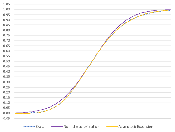
ℙ ( X t x ≤ y ) = ℙ ( X ^ t x ≤ y ) ℙ superscript subscript 𝑋 𝑡 𝑥 𝑦 ℙ superscript subscript ^ 𝑋 𝑡 𝑥 𝑦 \displaystyle\displaystyle\mathbb{P}(X_{t}^{x}\leq y)=\mathbb{P}(\hat{X}_{t}^{x}\leq y)
+ t H 𝔼 [ 𝟏 { X ^ t x ≤ y } ∑ j 1 , j 2 = 1 e ∑ i 1 , i 2 , i 3 = 1 d V i 1 V i 2 j 1 ( x ) V i 3 j 2 ( x ) A j 1 , j 2 − 1 ( x ) \displaystyle\displaystyle\hskip 15.00002pt+t^{H}\mathbb{E}\Bigl{[}{\bf 1}_{\left\{\hat{X}_{t}^{x}\leq y\right\}}\sum_{j_{1},j_{2}=1}^{e}\sum_{i_{1},i_{2},i_{3}=1}^{d}V_{i_{1}}V_{i_{2}}^{j_{1}}(x)V_{i_{3}}^{j_{2}}(x)A^{-1}_{j_{1},j_{2}}(x)
1 2 { B 1 H , i 1 B 1 H , i 2 B 1 H , i 3 − B 1 H , i 1 𝟏 i 1 = i 3 ≠ 0 − B 1 H , i 2 𝟏 i 2 = i 3 ≠ 0 } ] + O ( t 1 − H ) \displaystyle\displaystyle\hskip 45.00006pt\frac{1}{2}\{B_{1}^{H,i_{1}}B_{1}^{H,i_{2}}B_{1}^{H,i_{3}}-B_{1}^{H,i_{1}}{\bf 1}_{i_{1}=i_{3}\neq 0}-B_{1}^{H,i_{2}}{\bf 1}_{i_{2}=i_{3}\neq 0}\}\Bigr{]}+O(t^{1-H})\ \ (3.25)
or
ℙ ( X t x ≤ y ) = ℙ ( X ¯ t x ≤ y ) ℙ superscript subscript 𝑋 𝑡 𝑥 𝑦 ℙ superscript subscript ¯ 𝑋 𝑡 𝑥 𝑦 \displaystyle\displaystyle\mathbb{P}(X_{t}^{x}\leq y)=\mathbb{P}(\bar{X}_{t}^{x}\leq y)
+ 𝔼 [ 𝟏 { X ¯ t x ≤ y } ∑ j 1 , j 2 = 1 e ∑ i 1 , i 2 , i 3 = 1 d V i 1 V i 2 j 1 ( x ) V i 3 j 2 ( x ) A j 1 , j 2 − 1 ( x ) 1 t 2 H \displaystyle\displaystyle\hskip 15.00002pt+\mathbb{E}\Bigl{[}{\bf 1}_{\left\{\bar{X}_{t}^{x}\leq y\right\}}\sum_{j_{1},j_{2}=1}^{e}\sum_{i_{1},i_{2},i_{3}=1}^{d}V_{i_{1}}V_{i_{2}}^{j_{1}}(x)V_{i_{3}}^{j_{2}}(x)A^{-1}_{j_{1},j_{2}}(x)\frac{1}{t^{2H}}
1 2 { B t H , i 1 B t H , i 2 B t H , i 3 − B t H , i 1 t 2 H 𝟏 i 1 = i 3 ≠ 0 − B t H , i 2 t 2 H 𝟏 i 2 = i 3 ≠ 0 } ] + O ( t 1 − H ) , \displaystyle\displaystyle\hskip 45.00006pt\frac{1}{2}\{B_{t}^{H,i_{1}}B_{t}^{H,i_{2}}B_{t}^{H,i_{3}}-B_{t}^{H,i_{1}}t^{2H}{\bf 1}_{i_{1}=i_{3}\neq 0}-B_{t}^{H,i_{2}}t^{2H}{\bf 1}_{i_{2}=i_{3}\neq 0}\}\Bigr{]}+O(t^{1-H}),
where A ( x ) = ∑ i = 1 d V i ( x ) ⊗ V i ( x ) 𝐴 𝑥 superscript subscript 𝑖 1 𝑑 tensor-product subscript 𝑉 𝑖 𝑥 subscript 𝑉 𝑖 𝑥 \displaystyle A(x)=\sum_{i=1}^{d}V_{i}(x)\otimes V_{i}(x)
ℙ ( X t x ≤ y ) = ℙ ( X ^ t x ≤ y ) ℙ superscript subscript 𝑋 𝑡 𝑥 𝑦 ℙ superscript subscript ^ 𝑋 𝑡 𝑥 𝑦 \displaystyle\displaystyle\mathbb{P}(X_{t}^{x}\leq y)=\mathbb{P}(\hat{X}_{t}^{x}\leq y)
+ t H 𝔼 [ 𝟏 { X ^ t x ≤ y } ∑ j 1 , j 2 = 1 e ∑ i 1 , i 2 , i 3 = 1 d V i 1 V i 2 j 1 ( x ) V i 3 j 2 ( x ) A j 1 , j 2 − 1 ( x ) \displaystyle\displaystyle\hskip 15.00002pt+t^{H}\mathbb{E}\Bigl{[}{\bf 1}_{\left\{\hat{X}_{t}^{x}\leq y\right\}}\sum_{j_{1},j_{2}=1}^{e}\sum_{i_{1},i_{2},i_{3}=1}^{d}V_{i_{1}}V_{i_{2}}^{j_{1}}(x)V_{i_{3}}^{j_{2}}(x)A^{-1}_{j_{1},j_{2}}(x)
1 2 { B 1 H , i 1 B 1 H , i 2 B 1 H , i 3 − B 1 H , i 1 𝟏 i 1 = i 3 ≠ 0 − B 1 H , i 2 𝟏 i 2 = i 3 ≠ 0 } ] \displaystyle\displaystyle\hskip 45.00006pt\frac{1}{2}\{B_{1}^{H,i_{1}}B_{1}^{H,i_{2}}B_{1}^{H,i_{3}}-B_{1}^{H,i_{1}}{\bf 1}_{i_{1}=i_{3}\neq 0}-B_{1}^{H,i_{2}}{\bf 1}_{i_{2}=i_{3}\neq 0}\}\Bigr{]}
+ t 1 − H 𝔼 [ 𝟏 { X ^ t x ≤ y } ∑ j 1 , j 2 = 1 e ∑ i 1 = 1 d V 0 j 1 ( x ) V i 1 j 2 ( x ) A j 1 , j 2 − 1 ( x ) B 1 H , i 1 ] superscript 𝑡 1 𝐻 𝔼 delimited-[] subscript 1 superscript subscript ^ 𝑋 𝑡 𝑥 𝑦 superscript subscript subscript 𝑗 1 subscript 𝑗 2
1 𝑒 superscript subscript subscript 𝑖 1 1 𝑑 superscript subscript 𝑉 0 subscript 𝑗 1 𝑥 superscript subscript 𝑉 subscript 𝑖 1 subscript 𝑗 2 𝑥 subscript superscript 𝐴 1 subscript 𝑗 1 subscript 𝑗 2
𝑥 superscript subscript 𝐵 1 𝐻 subscript 𝑖 1
\displaystyle\displaystyle\hskip 15.00002pt+t^{1-H}\mathbb{E}\Bigl{[}{\bf 1}_{\left\{\hat{X}_{t}^{x}\leq y\right\}}\sum_{j_{1},j_{2}=1}^{e}\sum_{i_{1}=1}^{d}V_{0}^{j_{1}}(x)V_{i_{1}}^{j_{2}}(x)A^{-1}_{j_{1},j_{2}}(x)B_{1}^{H,i_{1}}\Bigr{]}
+ O ( t 2 H ) 𝑂 superscript 𝑡 2 𝐻 \displaystyle\displaystyle\hskip 15.00002pt+O(t^{2H}) (3.27)
or
ℙ ( X t x ≤ y ) = ℙ ( X ¯ t x ≤ y ) ℙ superscript subscript 𝑋 𝑡 𝑥 𝑦 ℙ superscript subscript ¯ 𝑋 𝑡 𝑥 𝑦 \displaystyle\displaystyle\mathbb{P}(X_{t}^{x}\leq y)=\mathbb{P}(\bar{X}_{t}^{x}\leq y)
+ 𝔼 [ 𝟏 { X ¯ t x ≤ y } ∑ j 1 , j 2 = 1 e ∑ i 1 , i 2 , i 3 = 1 d V i 1 V i 2 j 1 ( x ) V i 3 j 2 ( x ) A j 1 , j 2 − 1 ( x ) 1 t 2 H \displaystyle\displaystyle\hskip 15.00002pt+\mathbb{E}\Bigl{[}{\bf 1}_{\left\{\bar{X}_{t}^{x}\leq y\right\}}\sum_{j_{1},j_{2}=1}^{e}\sum_{i_{1},i_{2},i_{3}=1}^{d}V_{i_{1}}V_{i_{2}}^{j_{1}}(x)V_{i_{3}}^{j_{2}}(x)A^{-1}_{j_{1},j_{2}}(x)\frac{1}{t^{2H}}
1 2 { B t H , i 1 B t H , i 2 B t H , i 3 − B t H , i 1 t 2 H 𝟏 i 1 = i 3 ≠ 0 − B t H , i 2 t 2 H 𝟏 i 2 = i 3 ≠ 0 } ] \displaystyle\displaystyle\hskip 45.00006pt\frac{1}{2}\{B_{t}^{H,i_{1}}B_{t}^{H,i_{2}}B_{t}^{H,i_{3}}-B_{t}^{H,i_{1}}t^{2H}{\bf 1}_{i_{1}=i_{3}\neq 0}-B_{t}^{H,i_{2}}t^{2H}{\bf 1}_{i_{2}=i_{3}\neq 0}\}\Bigr{]}
+ 𝔼 [ 𝟏 { X ¯ t x ≤ y } ∑ j 1 , j 2 = 1 e ∑ i 1 = 1 d V 0 j 1 ( x ) V i 1 j 2 ( x ) A j 1 , j 2 − 1 ( x ) B t H , i 1 t t 2 H ] 𝔼 delimited-[] subscript 1 superscript subscript ¯ 𝑋 𝑡 𝑥 𝑦 superscript subscript subscript 𝑗 1 subscript 𝑗 2
1 𝑒 superscript subscript subscript 𝑖 1 1 𝑑 superscript subscript 𝑉 0 subscript 𝑗 1 𝑥 superscript subscript 𝑉 subscript 𝑖 1 subscript 𝑗 2 𝑥 subscript superscript 𝐴 1 subscript 𝑗 1 subscript 𝑗 2
𝑥 superscript subscript 𝐵 𝑡 𝐻 subscript 𝑖 1
𝑡 superscript 𝑡 2 𝐻 \displaystyle\displaystyle\hskip 15.00002pt+\mathbb{E}\Bigl{[}{\bf 1}_{\left\{\bar{X}_{t}^{x}\leq y\right\}}\sum_{j_{1},j_{2}=1}^{e}\sum_{i_{1}=1}^{d}V_{0}^{j_{1}}(x)V_{i_{1}}^{j_{2}}(x)A^{-1}_{j_{1},j_{2}}(x)\frac{B_{t}^{H,i_{1}}t}{t^{2H}}\Bigr{]}
+ O ( t 2 H ) . 𝑂 superscript 𝑡 2 𝐻 \displaystyle\displaystyle\hskip 15.00002pt+\ O(t^{2H}). (3.28)
Remark 4 .
The weight in Theorem 3
Remark 5 .
The expansion in Theorem 3
Remark 6 .
When e = d 𝑒 𝑑 \displaystyle e=d V ( ⋅ ) 𝑉 ⋅ \displaystyle V(\cdot)
Proof of Theorem 3 .
Hereafter, we use a notation ∫ 0 t u s i δ B s H , i := δ i ( u i 𝟏 [ 0 , t ] ( ⋅ ) ) assign superscript subscript 0 𝑡 superscript subscript 𝑢 𝑠 𝑖 𝛿 superscript subscript 𝐵 𝑠 𝐻 𝑖
superscript 𝛿 𝑖 superscript 𝑢 𝑖 subscript 1 0 𝑡 ⋅ \displaystyle\int_{0}^{t}u_{s}^{i}\delta B_{s}^{H,i}:=\delta^{i}(u^{i}{\bf 1}_{[0,t]}(\cdot)) i = 1 , … , d 𝑖 1 … 𝑑
\displaystyle i=1,\ldots,d u ∈ Dom δ H 𝑢 Dom subscript 𝛿 𝐻 \displaystyle u\in\mathrm{Dom}\delta_{H} O ( t 1 − H ) 𝑂 superscript 𝑡 1 𝐻 \displaystyle O(t^{1-H}) 2
𝔼 [ ∂ j f ( X ¯ t x ) V i 1 V i 2 j ( x ) 𝔹 ( i 1 , i 2 ) H ( t ) ] = ∫ ℝ d ∂ j f ( x + V ( x ) y ) V i 1 V i 2 j ( x ) 𝔼 [ δ y ( B t H ) 𝔹 ( i 1 , i 2 ) H ( t ) ] d y , 𝔼 delimited-[] subscript 𝑗 𝑓 subscript superscript ¯ 𝑋 𝑥 𝑡 subscript 𝑉 subscript 𝑖 1 superscript subscript 𝑉 subscript 𝑖 2 𝑗 𝑥 subscript superscript 𝔹 𝐻 subscript 𝑖 1 subscript 𝑖 2 𝑡 subscript superscript ℝ 𝑑 subscript 𝑗 𝑓 𝑥 𝑉 𝑥 𝑦 subscript 𝑉 subscript 𝑖 1 superscript subscript 𝑉 subscript 𝑖 2 𝑗 𝑥 𝔼 delimited-[] subscript 𝛿 𝑦 superscript subscript 𝐵 𝑡 𝐻 subscript superscript 𝔹 𝐻 subscript 𝑖 1 subscript 𝑖 2 𝑡 𝑑 𝑦 \displaystyle\displaystyle\mathbb{E}[\partial_{j}f(\bar{X}^{x}_{t})V_{i_{1}}V_{i_{2}}^{j}(x)\mathbb{B}^{H}_{(i_{1},i_{2})}(t)]=\int_{\mathbb{R}^{d}}\partial_{j}f(x+V(x)y)V_{i_{1}}V_{i_{2}}^{j}(x)\mathbb{E}[\delta_{y}(B_{t}^{H})\mathbb{B}^{H}_{(i_{1},i_{2})}(t)]dy, (3.29)
for j = 1 , … , e 𝑗 1 … 𝑒
\displaystyle j=1,\ldots,e i 1 , i 2 = 1 , … , d formulae-sequence subscript 𝑖 1 subscript 𝑖 2
1 … 𝑑
\displaystyle i_{1},i_{2}=1,\ldots,d [4 ] and the equation (4) in Song and Tindel (2021) [17 ] , it holds that
𝔹 ( i 1 , i 2 ) H ( t ) = ∫ 0 t ∫ 0 t 2 ∘ 𝑑 B t 1 H , i 1 ∘ 𝑑 B t 2 H , i 2 subscript superscript 𝔹 𝐻 subscript 𝑖 1 subscript 𝑖 2 𝑡 superscript subscript 0 𝑡 superscript subscript 0 subscript 𝑡 2 differential-d superscript subscript 𝐵 subscript 𝑡 1 𝐻 subscript 𝑖 1
differential-d superscript subscript 𝐵 subscript 𝑡 2 𝐻 subscript 𝑖 2
\displaystyle\displaystyle\mathbb{B}^{H}_{(i_{1},i_{2})}(t)=\int_{0}^{t}\int_{0}^{t_{2}}\circ dB_{t_{1}}^{H,i_{1}}\circ dB_{t_{2}}^{H,i_{2}} = \displaystyle\displaystyle= ∫ 0 t B s H , i 1 δ B s H , i 2 + H ∫ 0 t s 2 H − 1 𝑑 s 𝟏 i 1 = i 2 superscript subscript 0 𝑡 superscript subscript 𝐵 𝑠 𝐻 subscript 𝑖 1
𝛿 superscript subscript 𝐵 𝑠 𝐻 subscript 𝑖 2
𝐻 superscript subscript 0 𝑡 superscript 𝑠 2 𝐻 1 differential-d 𝑠 subscript 1 subscript 𝑖 1 subscript 𝑖 2 \displaystyle\displaystyle\int_{0}^{t}B_{s}^{H,i_{1}}\delta B_{s}^{H,i_{2}}+H\int_{0}^{t}s^{2H-1}ds{\bf 1}_{i_{1}=i_{2}} (3.30)
= \displaystyle\displaystyle= ∫ 0 t B s H , i 1 δ B s H , i 2 + 1 2 t 2 H 𝟏 i 1 = i 2 . superscript subscript 0 𝑡 superscript subscript 𝐵 𝑠 𝐻 subscript 𝑖 1
𝛿 superscript subscript 𝐵 𝑠 𝐻 subscript 𝑖 2
1 2 superscript 𝑡 2 𝐻 subscript 1 subscript 𝑖 1 subscript 𝑖 2 \displaystyle\displaystyle\int_{0}^{t}B_{s}^{H,i_{1}}\delta B_{s}^{H,i_{2}}+\frac{1}{2}t^{2H}{\bf 1}_{i_{1}=i_{2}}.
Then, we have
𝔼 [ δ y ( B t H ) 𝔹 ( i 1 , i 2 ) H ( t ) ] = 𝔼 [ δ y ( B t H ) ∫ 0 t B s H , i 1 δ B s H , i 2 ] + 𝔼 [ δ y ( B t H ) ] 1 2 t 2 H 𝟏 i 1 = i 2 . 𝔼 delimited-[] subscript 𝛿 𝑦 superscript subscript 𝐵 𝑡 𝐻 subscript superscript 𝔹 𝐻 subscript 𝑖 1 subscript 𝑖 2 𝑡 𝔼 delimited-[] subscript 𝛿 𝑦 superscript subscript 𝐵 𝑡 𝐻 superscript subscript 0 𝑡 superscript subscript 𝐵 𝑠 𝐻 subscript 𝑖 1
𝛿 superscript subscript 𝐵 𝑠 𝐻 subscript 𝑖 2
𝔼 delimited-[] subscript 𝛿 𝑦 superscript subscript 𝐵 𝑡 𝐻 1 2 superscript 𝑡 2 𝐻 subscript 1 subscript 𝑖 1 subscript 𝑖 2 \displaystyle\displaystyle\mathbb{E}[\delta_{y}(B_{t}^{H})\mathbb{B}^{H}_{(i_{1},i_{2})}(t)]=\mathbb{E}[\delta_{y}(B_{t}^{H})\int_{0}^{t}B_{s}^{H,i_{1}}\delta B_{s}^{H,i_{2}}]+\mathbb{E}[\delta_{y}(B_{t}^{H})]\frac{1}{2}t^{2H}{\bf 1}_{i_{1}=i_{2}}. (3.31)
Then we compute the Malliavin derivatives of ∫ 0 t B s H , i 1 δ B s H , i 2 superscript subscript 0 𝑡 superscript subscript 𝐵 𝑠 𝐻 subscript 𝑖 1
𝛿 superscript subscript 𝐵 𝑠 𝐻 subscript 𝑖 2
\displaystyle\int_{0}^{t}B_{s}^{H,i_{1}}\delta B_{s}^{H,i_{2}}
𝔼 [ D 0 ∫ 0 t B s H , i 1 δ B s H , i 2 ] = 𝔼 [ ∫ 0 t B s H , i 1 δ B s H , i 2 ] = 0 . 𝔼 delimited-[] superscript 𝐷 0 superscript subscript 0 𝑡 superscript subscript 𝐵 𝑠 𝐻 subscript 𝑖 1
𝛿 superscript subscript 𝐵 𝑠 𝐻 subscript 𝑖 2
𝔼 delimited-[] superscript subscript 0 𝑡 superscript subscript 𝐵 𝑠 𝐻 subscript 𝑖 1
𝛿 superscript subscript 𝐵 𝑠 𝐻 subscript 𝑖 2
0 \displaystyle\displaystyle\mathbb{E}[D^{0}\int_{0}^{t}B_{s}^{H,i_{1}}\delta B_{s}^{H,i_{2}}]=\mathbb{E}[\int_{0}^{t}B_{s}^{H,i_{1}}\delta B_{s}^{H,i_{2}}]=0. (3.32)
First we compute 𝔼 [ D ∫ 0 t B s H , i 1 δ B s H , i 2 ] = ( 𝔼 [ D ⋅ 1 ∫ 0 t B s H , i 1 δ B s H , i 2 ] , … , 𝔼 [ D ⋅ d ∫ 0 t B s H , i 1 δ B s H , i 2 ] ) 𝔼 delimited-[] 𝐷 superscript subscript 0 𝑡 superscript subscript 𝐵 𝑠 𝐻 subscript 𝑖 1
𝛿 superscript subscript 𝐵 𝑠 𝐻 subscript 𝑖 2
𝔼 delimited-[] subscript superscript 𝐷 1 ⋅ superscript subscript 0 𝑡 superscript subscript 𝐵 𝑠 𝐻 subscript 𝑖 1
𝛿 superscript subscript 𝐵 𝑠 𝐻 subscript 𝑖 2
… 𝔼 delimited-[] subscript superscript 𝐷 𝑑 ⋅ superscript subscript 0 𝑡 superscript subscript 𝐵 𝑠 𝐻 subscript 𝑖 1
𝛿 superscript subscript 𝐵 𝑠 𝐻 subscript 𝑖 2
\displaystyle\mathbb{E}[D\int_{0}^{t}B_{s}^{H,i_{1}}\delta B_{s}^{H,i_{2}}]=(\mathbb{E}[D^{1}_{\cdot}\int_{0}^{t}B_{s}^{H,i_{1}}\delta B_{s}^{H,i_{2}}],\ldots,\mathbb{E}[D^{d}_{\cdot}\int_{0}^{t}B_{s}^{H,i_{1}}\delta B_{s}^{H,i_{2}}]) ℓ = 1 , … , d ℓ 1 … 𝑑
\displaystyle\ell=1,\ldots,d
D r ℓ ∫ 0 t B s H , i 1 δ B s H , i 2 subscript superscript 𝐷 ℓ 𝑟 superscript subscript 0 𝑡 superscript subscript 𝐵 𝑠 𝐻 subscript 𝑖 1
𝛿 superscript subscript 𝐵 𝑠 𝐻 subscript 𝑖 2
\displaystyle\displaystyle D^{\ell}_{r}\int_{0}^{t}B_{s}^{H,i_{1}}\delta B_{s}^{H,i_{2}} = \displaystyle\displaystyle= B r H , i 1 𝟏 ℓ = i 2 + ∫ r t D r ℓ B s H , i 1 δ B s H , i 2 superscript subscript 𝐵 𝑟 𝐻 subscript 𝑖 1
subscript 1 ℓ subscript 𝑖 2 superscript subscript 𝑟 𝑡 superscript subscript 𝐷 𝑟 ℓ superscript subscript 𝐵 𝑠 𝐻 subscript 𝑖 1
𝛿 superscript subscript 𝐵 𝑠 𝐻 subscript 𝑖 2
\displaystyle\displaystyle B_{r}^{H,i_{1}}{\bf 1}_{\ell=i_{2}}+\int_{r}^{t}D_{r}^{\ell}B_{s}^{H,i_{1}}\delta B_{s}^{H,i_{2}} (3.33)
= \displaystyle\displaystyle= B r H , i 1 𝟏 ℓ = i 2 + ( B t H , i 2 − B r H , i 2 ) 𝟏 ℓ = i 1 for r ≤ t superscript subscript 𝐵 𝑟 𝐻 subscript 𝑖 1
subscript 1 ℓ subscript 𝑖 2 superscript subscript 𝐵 𝑡 𝐻 subscript 𝑖 2
superscript subscript 𝐵 𝑟 𝐻 subscript 𝑖 2
subscript 1 ℓ subscript 𝑖 1 for 𝑟
𝑡 \displaystyle\displaystyle B_{r}^{H,i_{1}}{\bf 1}_{\ell=i_{2}}+(B_{t}^{H,i_{2}}-B_{r}^{H,i_{2}}){\bf 1}_{\ell=i_{1}}\ \ \ \mbox{for}\ r\leq t\ \
and then
𝔼 [ D r ℓ ∫ 0 t B s H , i 1 δ B s H , i 2 ] = 0 for r ≤ t , formulae-sequence 𝔼 delimited-[] subscript superscript 𝐷 ℓ 𝑟 superscript subscript 0 𝑡 superscript subscript 𝐵 𝑠 𝐻 subscript 𝑖 1
𝛿 superscript subscript 𝐵 𝑠 𝐻 subscript 𝑖 2
0 for 𝑟 𝑡 \displaystyle\displaystyle\mathbb{E}[D^{\ell}_{r}\int_{0}^{t}B_{s}^{H,i_{1}}\delta B_{s}^{H,i_{2}}]=0\ \ \ \mbox{for}\ r\leq t, (3.34)
i.e. 𝔼 [ D 1 ∫ 0 t B s H , i 1 δ B s H , i 2 ] = 𝔼 [ D ∫ 0 t B s H , i 1 δ B s H , i 2 ] = 0 𝔼 delimited-[] superscript 𝐷 1 superscript subscript 0 𝑡 superscript subscript 𝐵 𝑠 𝐻 subscript 𝑖 1
𝛿 superscript subscript 𝐵 𝑠 𝐻 subscript 𝑖 2
𝔼 delimited-[] 𝐷 superscript subscript 0 𝑡 superscript subscript 𝐵 𝑠 𝐻 subscript 𝑖 1
𝛿 superscript subscript 𝐵 𝑠 𝐻 subscript 𝑖 2
0 \displaystyle\mathbb{E}[D^{1}\int_{0}^{t}B_{s}^{H,i_{1}}\delta B_{s}^{H,i_{2}}]=\mathbb{E}[D\int_{0}^{t}B_{s}^{H,i_{1}}\delta B_{s}^{H,i_{2}}]=0 1 2 𝔼 [ D 2 ∫ 0 t B s H , i 1 δ B s H , i 2 ] 1 2 𝔼 delimited-[] superscript 𝐷 2 superscript subscript 0 𝑡 superscript subscript 𝐵 𝑠 𝐻 subscript 𝑖 1
𝛿 superscript subscript 𝐵 𝑠 𝐻 subscript 𝑖 2
\displaystyle\frac{1}{2}\mathbb{E}[D^{2}\int_{0}^{t}B_{s}^{H,i_{1}}\delta B_{s}^{H,i_{2}}] D 2 ∫ 0 t B s H , i 1 δ B s H , i 2 superscript 𝐷 2 superscript subscript 0 𝑡 superscript subscript 𝐵 𝑠 𝐻 subscript 𝑖 1
𝛿 superscript subscript 𝐵 𝑠 𝐻 subscript 𝑖 2
\displaystyle D^{2}\int_{0}^{t}B_{s}^{H,i_{1}}\delta B_{s}^{H,i_{2}}
D t 1 ℓ 1 D t 2 ℓ 2 ∫ 0 t B s H , i 1 δ B s H , i 2 subscript superscript 𝐷 subscript ℓ 1 subscript 𝑡 1 subscript superscript 𝐷 subscript ℓ 2 subscript 𝑡 2 superscript subscript 0 𝑡 superscript subscript 𝐵 𝑠 𝐻 subscript 𝑖 1
𝛿 superscript subscript 𝐵 𝑠 𝐻 subscript 𝑖 2
\displaystyle\displaystyle D^{\ell_{1}}_{t_{1}}D^{\ell_{2}}_{t_{2}}\int_{0}^{t}B_{s}^{H,i_{1}}\delta B_{s}^{H,i_{2}}
= \displaystyle\displaystyle= D t 1 ℓ 1 ( B t 2 H , i 1 𝟏 ℓ 2 = i 2 + ( B t H , i 2 − B t 2 H , i 2 ) 𝟏 ℓ 2 = i 1 ) subscript superscript 𝐷 subscript ℓ 1 subscript 𝑡 1 superscript subscript 𝐵 subscript 𝑡 2 𝐻 subscript 𝑖 1
subscript 1 subscript ℓ 2 subscript 𝑖 2 superscript subscript 𝐵 𝑡 𝐻 subscript 𝑖 2
superscript subscript 𝐵 subscript 𝑡 2 𝐻 subscript 𝑖 2
subscript 1 subscript ℓ 2 subscript 𝑖 1 \displaystyle\displaystyle D^{\ell_{1}}_{t_{1}}(B_{t_{2}}^{H,i_{1}}{\bf 1}_{\ell_{2}=i_{2}}+(B_{t}^{H,i_{2}}-B_{t_{2}}^{H,i_{2}}){\bf 1}_{\ell_{2}=i_{1}})
= \displaystyle\displaystyle= 𝟏 0 ≤ t 1 ≤ t 2 ≤ t 𝟏 ℓ 1 = i 1 𝟏 ℓ 2 = i 2 + 𝟏 0 ≤ t 1 , t 2 ≤ t 𝟏 ℓ 1 = i 2 𝟏 ℓ 2 = i 1 − 𝟏 0 ≤ t 1 ≤ t 2 ≤ t 𝟏 ℓ 1 = i 2 𝟏 ℓ 2 = i 1 , ℓ 1 , ℓ 2 = 1 , … , d , formulae-sequence subscript 1 0 subscript 𝑡 1 subscript 𝑡 2 𝑡 subscript 1 subscript ℓ 1 subscript 𝑖 1 subscript 1 subscript ℓ 2 subscript 𝑖 2 subscript 1 formulae-sequence 0 subscript 𝑡 1 subscript 𝑡 2 𝑡 subscript 1 subscript ℓ 1 subscript 𝑖 2 subscript 1 subscript ℓ 2 subscript 𝑖 1 subscript 1 0 subscript 𝑡 1 subscript 𝑡 2 𝑡 subscript 1 subscript ℓ 1 subscript 𝑖 2 subscript 1 subscript ℓ 2 subscript 𝑖 1 subscript ℓ 1 subscript ℓ 2
1 … 𝑑
\displaystyle\displaystyle{\bf 1}_{0\leq t_{1}\leq t_{2}\leq t}{\bf 1}_{\ell_{1}=i_{1}}{\bf 1}_{\ell_{2}=i_{2}}+{\bf 1}_{0\leq t_{1},t_{2}\leq t}{\bf 1}_{\ell_{1}=i_{2}}{\bf 1}_{\ell_{2}=i_{1}}-{\bf 1}_{0\leq t_{1}\leq t_{2}\leq t}{\bf 1}_{\ell_{1}=i_{2}}{\bf 1}_{\ell_{2}=i_{1}},\ \ \ell_{1},\ell_{2}=1,\ldots,d,
from (3.33 ℓ 1 , ℓ 2 = 1 , … , d formulae-sequence subscript ℓ 1 subscript ℓ 2
1 … 𝑑
\displaystyle\ell_{1},\ell_{2}=1,\ldots,d ( t 1 , t 2 ) ↦ 𝔼 [ D t 1 ℓ 1 D t 2 ℓ 2 ∫ 0 t B s H , i 1 δ B s H , i 2 ] maps-to subscript 𝑡 1 subscript 𝑡 2 𝔼 delimited-[] subscript superscript 𝐷 subscript ℓ 1 subscript 𝑡 1 subscript superscript 𝐷 subscript ℓ 2 subscript 𝑡 2 superscript subscript 0 𝑡 superscript subscript 𝐵 𝑠 𝐻 subscript 𝑖 1
𝛿 superscript subscript 𝐵 𝑠 𝐻 subscript 𝑖 2
\displaystyle(t_{1},t_{2})\mapsto\mathbb{E}[D^{\ell_{1}}_{t_{1}}D^{\ell_{2}}_{t_{2}}\int_{0}^{t}B_{s}^{H,i_{1}}\delta B_{s}^{H,i_{2}}]
( t 1 , t 2 ) ↦ maps-to subscript 𝑡 1 subscript 𝑡 2 absent \displaystyle\displaystyle(t_{1},t_{2})\mapsto 𝔼 [ D t 1 ℓ 1 D t 2 ℓ 2 ∫ 0 t B s H , i 1 δ B s H , i 2 ] 𝔼 delimited-[] subscript superscript 𝐷 subscript ℓ 1 subscript 𝑡 1 subscript superscript 𝐷 subscript ℓ 2 subscript 𝑡 2 superscript subscript 0 𝑡 superscript subscript 𝐵 𝑠 𝐻 subscript 𝑖 1
𝛿 superscript subscript 𝐵 𝑠 𝐻 subscript 𝑖 2
\displaystyle\displaystyle\ \ \mathbb{E}[D^{\ell_{1}}_{t_{1}}D^{\ell_{2}}_{t_{2}}\int_{0}^{t}B_{s}^{H,i_{1}}\delta B_{s}^{H,i_{2}}]
= 𝟏 [ 0 , t 2 ] ( t 1 ) 𝟏 [ 0 , t ] ( t 2 ) 𝟏 ℓ 1 = i 1 𝟏 ℓ 2 = i 2 + ( 𝟏 [ 0 , t ] ( t 1 ) − 𝟏 [ 0 , t 2 ] ( t 1 ) ) 𝟏 [ 0 , t ] ( t 2 ) 𝟏 ℓ 1 = i 2 𝟏 ℓ 2 = i 1 , absent subscript 1 0 subscript 𝑡 2 subscript 𝑡 1 subscript 1 0 𝑡 subscript 𝑡 2 subscript 1 subscript ℓ 1 subscript 𝑖 1 subscript 1 subscript ℓ 2 subscript 𝑖 2 subscript 1 0 𝑡 subscript 𝑡 1 subscript 1 0 subscript 𝑡 2 subscript 𝑡 1 subscript 1 0 𝑡 subscript 𝑡 2 subscript 1 subscript ℓ 1 subscript 𝑖 2 subscript 1 subscript ℓ 2 subscript 𝑖 1 \displaystyle\displaystyle={\bf 1}_{[0,t_{2}]}(t_{1}){\bf 1}_{[0,t]}(t_{2}){\bf 1}_{\ell_{1}=i_{1}}{\bf 1}_{\ell_{2}=i_{2}}+({\bf 1}_{[0,t]}(t_{1})-{\bf 1}_{[0,t_{2}]}(t_{1})){\bf 1}_{[0,t]}(t_{2}){\bf 1}_{\ell_{1}=i_{2}}{\bf 1}_{\ell_{2}=i_{1}}, (3.36)
and for 𝟏 [ 0 , t ] e ℓ 1 , 𝟏 [ 0 , t ] e ℓ 2 ∈ ℋ ¯ d subscript 1 0 𝑡 subscript 𝑒 subscript ℓ 1 subscript 1 0 𝑡 subscript 𝑒 subscript ℓ 2
superscript ¯ ℋ 𝑑 \displaystyle{\bf 1}_{[0,t]}e_{\ell_{1}},{\bf 1}_{[0,t]}e_{\ell_{2}}\in\bar{\cal H}^{d}
⟨ 𝟏 [ 0 , t ] e ℓ 1 ⊗ 𝟏 [ 0 , t ] e ℓ 2 , 𝔼 [ D 2 ∫ 0 t B s H , i 1 δ B s H , i 2 ] ⟩ ( ℋ ¯ d ) ⊗ 2 subscript tensor-product subscript 1 0 𝑡 subscript 𝑒 subscript ℓ 1 subscript 1 0 𝑡 subscript 𝑒 subscript ℓ 2 𝔼 delimited-[] superscript 𝐷 2 superscript subscript 0 𝑡 superscript subscript 𝐵 𝑠 𝐻 subscript 𝑖 1
𝛿 superscript subscript 𝐵 𝑠 𝐻 subscript 𝑖 2
superscript superscript ¯ ℋ 𝑑 tensor-product absent 2 \displaystyle\displaystyle\Big{\langle}{\bf 1}_{[0,t]}e_{\ell_{1}}\otimes{\bf 1}_{[0,t]}e_{\ell_{2}},\mathbb{E}[D^{2}\int_{0}^{t}B_{s}^{H,i_{1}}\delta B_{s}^{H,i_{2}}]\Big{\rangle}_{(\bar{\cal H}^{d})^{\otimes 2}}
= \displaystyle\displaystyle= ∫ 0 t ∫ 0 t K H ( t , t 1 ) 𝟏 [ 0 , t ] ( t 1 ) K H ( t , t 2 ) 𝟏 [ 0 , t ] ( t 2 ) { K H ( t 2 , t 1 ) 𝟏 [ 0 , t 2 ] ( t 1 ) K H ( t , t 2 ) 𝟏 [ 0 , t ] ( t 2 ) 𝟏 ℓ 1 = i 1 𝟏 ℓ 2 = i 2 \displaystyle\displaystyle\int_{0}^{t}\int_{0}^{t}K_{H}(t,t_{1}){\bf 1}_{[0,t]}(t_{1})K_{H}(t,t_{2}){\bf 1}_{[0,t]}(t_{2})\Big{\{}K_{H}(t_{2},t_{1}){\bf 1}_{[0,t_{2}]}(t_{1})K_{H}(t,t_{2}){\bf 1}_{[0,t]}(t_{2}){\bf 1}_{\ell_{1}=i_{1}}{\bf 1}_{\ell_{2}=i_{2}}
+ { K H ( t , t 1 ) 𝟏 [ 0 , t ] ( t 1 ) − K H ( t 2 , t 1 ) 𝟏 [ 0 , t 2 ] ( t 1 ) } K H ( t , t 2 ) 𝟏 [ 0 , t ] ( t 2 ) 𝟏 ℓ 1 = i 2 𝟏 ℓ 2 = i 1 } d t 1 d t 2 . \displaystyle\displaystyle~{}~{}~{}~{}~{}~{}~{}~{}~{}~{}~{}~{}~{}~{}~{}+\{K_{H}(t,t_{1}){\bf 1}_{[0,t]}(t_{1})-K_{H}(t_{2},t_{1}){\bf 1}_{[0,t_{2}]}(t_{1})\}K_{H}(t,t_{2}){\bf 1}_{[0,t]}(t_{2}){\bf 1}_{\ell_{1}=i_{2}}{\bf 1}_{\ell_{2}=i_{1}}\Big{\}}dt_{1}dt_{2}. (3.37)
We note
1 p ! 𝔼 [ D p ∫ 0 t B s H , i 1 δ B s H , i 2 ] = 0 , p ≥ 3 . formulae-sequence 1 𝑝 𝔼 delimited-[] superscript 𝐷 𝑝 superscript subscript 0 𝑡 superscript subscript 𝐵 𝑠 𝐻 subscript 𝑖 1
𝛿 superscript subscript 𝐵 𝑠 𝐻 subscript 𝑖 2
0 𝑝 3 \displaystyle\displaystyle\frac{1}{p!}\mathbb{E}[D^{p}\int_{0}^{t}B_{s}^{H,i_{1}}\delta B_{s}^{H,i_{2}}]=0,\ \ p\geq 3. (3.38)
Thus, we only need to compute the following term:
∑ γ 1 , γ 2 = 1 d 𝔼 [ ∂ γ 1 ∂ γ 2 δ y ( B t H ) ⟨ D B t H , γ 1 ⊗ D B t H , γ 2 , 1 2 ! 𝔼 [ D 2 ∫ 0 t B s H , i 1 δ B s H , i 2 ] ⟩ ( ℋ ¯ d ) ⊗ 2 ] . superscript subscript subscript 𝛾 1 subscript 𝛾 2
1 𝑑 𝔼 delimited-[] subscript subscript 𝛾 1 subscript subscript 𝛾 2 subscript 𝛿 𝑦 superscript subscript 𝐵 𝑡 𝐻 subscript tensor-product 𝐷 superscript subscript 𝐵 𝑡 𝐻 subscript 𝛾 1
𝐷 superscript subscript 𝐵 𝑡 𝐻 subscript 𝛾 2
1 2 𝔼 delimited-[] superscript 𝐷 2 superscript subscript 0 𝑡 superscript subscript 𝐵 𝑠 𝐻 subscript 𝑖 1
𝛿 superscript subscript 𝐵 𝑠 𝐻 subscript 𝑖 2
superscript superscript ¯ ℋ 𝑑 tensor-product absent 2 \displaystyle\displaystyle\sum_{\gamma_{1},\gamma_{2}=1}^{d}\mathbb{E}[\partial_{\gamma_{1}}\partial_{\gamma_{2}}\delta_{y}(B_{t}^{H})\langle DB_{t}^{H,\gamma_{1}}\otimes DB_{t}^{H,\gamma_{2}},\frac{1}{2!}\mathbb{E}[D^{2}\int_{0}^{t}B_{s}^{H,i_{1}}\delta B_{s}^{H,i_{2}}]\rangle_{(\bar{\cal H}^{d})^{\otimes 2}}]. (3.39)
Since D ⋅ ℓ B t H , i = 𝟏 [ 0 , t ] ( ⋅ ) 𝟏 ℓ = i subscript superscript 𝐷 ℓ ⋅ superscript subscript 𝐵 𝑡 𝐻 𝑖
subscript 1 0 𝑡 ⋅ subscript 1 ℓ 𝑖 \displaystyle D^{\ell}_{\cdot}B_{t}^{H,i}={\bf 1}_{[0,t]}(\cdot){\bf 1}_{\ell=i} i , ℓ = 1 , … , d formulae-sequence 𝑖 ℓ
1 … 𝑑
\displaystyle i,\ell=1,\ldots,d
∑ γ 1 , γ 2 = 1 d 𝔼 [ ∂ γ 1 ∂ γ 2 δ y ( B t H ) ⟨ D B t H , γ 1 ⊗ D B t H , γ 2 , 1 2 ! 𝔼 [ D 2 ∫ 0 t B s H , i 1 δ B s H , i 2 ] ⟩ ( ℋ ¯ d ) ⊗ 2 ] superscript subscript subscript 𝛾 1 subscript 𝛾 2
1 𝑑 𝔼 delimited-[] subscript subscript 𝛾 1 subscript subscript 𝛾 2 subscript 𝛿 𝑦 superscript subscript 𝐵 𝑡 𝐻 subscript tensor-product 𝐷 superscript subscript 𝐵 𝑡 𝐻 subscript 𝛾 1
𝐷 superscript subscript 𝐵 𝑡 𝐻 subscript 𝛾 2
1 2 𝔼 delimited-[] superscript 𝐷 2 superscript subscript 0 𝑡 superscript subscript 𝐵 𝑠 𝐻 subscript 𝑖 1
𝛿 superscript subscript 𝐵 𝑠 𝐻 subscript 𝑖 2
superscript superscript ¯ ℋ 𝑑 tensor-product absent 2 \displaystyle\displaystyle\sum_{\gamma_{1},\gamma_{2}=1}^{d}\mathbb{E}[\partial_{\gamma_{1}}\partial_{\gamma_{2}}\delta_{y}(B_{t}^{H})\langle DB_{t}^{H,\gamma_{1}}\otimes DB_{t}^{H,\gamma_{2}},\frac{1}{2!}\mathbb{E}[D^{2}\int_{0}^{t}B_{s}^{H,i_{1}}\delta B_{s}^{H,i_{2}}]\rangle_{(\bar{\cal H}^{d})^{\otimes 2}}]
= \displaystyle\displaystyle= ∑ γ 1 , γ 2 = 1 d 𝔼 [ ∂ γ 1 ∂ γ 2 δ y ( B t H ) 1 2 ! ∑ ℓ 1 , ℓ 2 = 1 d ∫ 0 t ∫ 0 t K H ( t , t 1 ) 𝟏 [ 0 , t ] ( t 1 ) 𝟏 ℓ 1 = γ 1 K H ( t , t 2 ) 𝟏 [ 0 , t ] ( t 2 ) 𝟏 ℓ 2 = γ 2 \displaystyle\displaystyle\sum_{\gamma_{1},\gamma_{2}=1}^{d}\mathbb{E}[\partial_{\gamma_{1}}\partial_{\gamma_{2}}\delta_{y}(B_{t}^{H})\frac{1}{2!}\sum_{\ell_{1},\ell_{2}=1}^{d}\int_{0}^{t}\int_{0}^{t}K_{H}(t,t_{1}){\bf 1}_{[0,t]}(t_{1}){\bf 1}_{\ell_{1}=\gamma_{1}}K_{H}(t,t_{2}){\bf 1}_{[0,t]}(t_{2}){\bf 1}_{\ell_{2}=\gamma_{2}}
K H ( t , t 2 ) 𝟏 [ 0 , t ] ( t 2 ) { K H ( t 2 , t 1 ) 𝟏 [ 0 , t 2 ] ( t 1 ) 𝟏 ℓ 1 = i 1 𝟏 ℓ 2 = i 2 \displaystyle\displaystyle\hskip 112.50017ptK_{H}(t,t_{2}){\bf 1}_{[0,t]}(t_{2})\{K_{H}(t_{2},t_{1}){\bf 1}_{[0,t_{2}]}(t_{1}){\bf 1}_{\ell_{1}=i_{1}}{\bf 1}_{\ell_{2}=i_{2}}
+ { K H ( t , t 1 ) 𝟏 [ 0 , t ] ( t 1 ) − K H ( t 2 , t 1 ) 𝟏 [ 0 , t 2 ] ( t 1 ) } 𝟏 ℓ 1 = i 2 𝟏 ℓ 2 = i 1 } d t 1 d t 2 ] \displaystyle\displaystyle\hskip 115.00017pt+\{K_{H}(t,t_{1}){\bf 1}_{[0,t]}(t_{1})-K_{H}(t_{2},t_{1}){\bf 1}_{[0,t_{2}]}(t_{1})\}{\bf 1}_{\ell_{1}=i_{2}}{\bf 1}_{\ell_{2}=i_{1}}\}dt_{1}dt_{2}]
= \displaystyle\displaystyle= 𝔼 [ ∂ i 1 ∂ i 2 δ y ( B t H ) ] 1 2 ∫ 0 t ∫ 0 t K H ( t , t 1 ) K H ( t , t 2 ) 2 K H ( t 2 , t 1 ) 𝟏 [ 0 , t 2 ] ( t 1 ) 𝑑 t 1 𝑑 t 2 𝔼 delimited-[] subscript subscript 𝑖 1 subscript subscript 𝑖 2 subscript 𝛿 𝑦 superscript subscript 𝐵 𝑡 𝐻 1 2 superscript subscript 0 𝑡 superscript subscript 0 𝑡 subscript 𝐾 𝐻 𝑡 subscript 𝑡 1 subscript 𝐾 𝐻 superscript 𝑡 subscript 𝑡 2 2 subscript 𝐾 𝐻 subscript 𝑡 2 subscript 𝑡 1 subscript 1 0 subscript 𝑡 2 subscript 𝑡 1 differential-d subscript 𝑡 1 differential-d subscript 𝑡 2 \displaystyle\displaystyle\mathbb{E}[\partial_{i_{1}}\partial_{i_{2}}\delta_{y}(B_{t}^{H})]\frac{1}{2}\int_{0}^{t}\int_{0}^{t}K_{H}(t,t_{1})K_{H}(t,t_{2})^{2}K_{H}(t_{2},t_{1}){\bf 1}_{[0,t_{2}]}(t_{1})dt_{1}dt_{2}
+ 𝔼 [ ∂ i 2 ∂ i 1 δ y ( B t H ) ] 1 2 ∫ 0 t ∫ 0 t K H ( t , t 1 ) K H ( t , t 2 ) 2 { K H ( t , t 1 ) − K H ( t 2 , t 1 ) 𝟏 [ 0 , t 2 ] ( t 1 ) } 𝑑 t 1 𝑑 t 2 . 𝔼 delimited-[] subscript subscript 𝑖 2 subscript subscript 𝑖 1 subscript 𝛿 𝑦 superscript subscript 𝐵 𝑡 𝐻 1 2 superscript subscript 0 𝑡 superscript subscript 0 𝑡 subscript 𝐾 𝐻 𝑡 subscript 𝑡 1 subscript 𝐾 𝐻 superscript 𝑡 subscript 𝑡 2 2 subscript 𝐾 𝐻 𝑡 subscript 𝑡 1 subscript 𝐾 𝐻 subscript 𝑡 2 subscript 𝑡 1 subscript 1 0 subscript 𝑡 2 subscript 𝑡 1 differential-d subscript 𝑡 1 differential-d subscript 𝑡 2 \displaystyle\displaystyle+\mathbb{E}[\partial_{i_{2}}\partial_{i_{1}}\delta_{y}(B_{t}^{H})]\frac{1}{2}\int_{0}^{t}\int_{0}^{t}K_{H}(t,t_{1})K_{H}(t,t_{2})^{2}\{K_{H}(t,t_{1})-K_{H}(t_{2},t_{1}){\bf 1}_{[0,t_{2}]}(t_{1})\}dt_{1}dt_{2}. (3.40)
Here, we note that
𝔼 [ ∂ i 1 ∂ i 2 δ y ( B t H ) ] = 𝔼 [ ∂ i 2 ∂ i 1 δ y ( B t H ) ] 𝔼 delimited-[] subscript subscript 𝑖 1 subscript subscript 𝑖 2 subscript 𝛿 𝑦 superscript subscript 𝐵 𝑡 𝐻 𝔼 delimited-[] subscript subscript 𝑖 2 subscript subscript 𝑖 1 subscript 𝛿 𝑦 superscript subscript 𝐵 𝑡 𝐻 \displaystyle\displaystyle\mathbb{E}[\partial_{i_{1}}\partial_{i_{2}}\delta_{y}(B_{t}^{H})]=\mathbb{E}[\partial_{i_{2}}\partial_{i_{1}}\delta_{y}(B_{t}^{H})]
= \displaystyle\displaystyle= 𝔼 [ δ y ( B t H ) H ( i 1 , i 2 ) ( B t H , 1 ) ] ( = 𝔼 [ δ y ( B t H ) H ( i 2 , i 1 ) ( B t H , 1 ) ] ) annotated 𝔼 delimited-[] subscript 𝛿 𝑦 superscript subscript 𝐵 𝑡 𝐻 subscript 𝐻 subscript 𝑖 1 subscript 𝑖 2 superscript subscript 𝐵 𝑡 𝐻 1 absent 𝔼 delimited-[] subscript 𝛿 𝑦 superscript subscript 𝐵 𝑡 𝐻 subscript 𝐻 subscript 𝑖 2 subscript 𝑖 1 superscript subscript 𝐵 𝑡 𝐻 1 \displaystyle\displaystyle\mathbb{E}[\delta_{y}(B_{t}^{H})H_{(i_{1},i_{2})}(B_{t}^{H},1)]\ (=\mathbb{E}[\delta_{y}(B_{t}^{H})H_{(i_{2},i_{1})}(B_{t}^{H},1)])
= \displaystyle\displaystyle= 𝔼 [ δ y ( B t H ) 1 t 4 H { B t H , i 1 B t H , i 2 − t 2 H 𝟏 i 1 = i 2 } ] . 𝔼 delimited-[] subscript 𝛿 𝑦 superscript subscript 𝐵 𝑡 𝐻 1 superscript 𝑡 4 𝐻 superscript subscript 𝐵 𝑡 𝐻 subscript 𝑖 1
superscript subscript 𝐵 𝑡 𝐻 subscript 𝑖 2
superscript 𝑡 2 𝐻 subscript 1 subscript 𝑖 1 subscript 𝑖 2 \displaystyle\displaystyle\mathbb{E}[\delta_{y}(B_{t}^{H})\frac{1}{t^{4H}}\{B_{t}^{H,i_{1}}B_{t}^{H,i_{2}}-t^{2H}{\bf 1}_{i_{1}=i_{2}}\}]. (3.41)
Therefore, we obtain
∑ γ 1 , γ 2 = 1 d 𝔼 [ ∂ γ 1 ∂ γ 2 δ y ( B t H ) ⟨ D B t H , γ 1 ⊗ D B t H , γ 2 , 1 2 ! 𝔼 [ D 2 ∫ 0 t B s H , i 1 δ B s H , i 2 ] ⟩ ( ℋ ¯ d ) ⊗ 2 ] superscript subscript subscript 𝛾 1 subscript 𝛾 2
1 𝑑 𝔼 delimited-[] subscript subscript 𝛾 1 subscript subscript 𝛾 2 subscript 𝛿 𝑦 superscript subscript 𝐵 𝑡 𝐻 subscript tensor-product 𝐷 superscript subscript 𝐵 𝑡 𝐻 subscript 𝛾 1
𝐷 superscript subscript 𝐵 𝑡 𝐻 subscript 𝛾 2
1 2 𝔼 delimited-[] superscript 𝐷 2 superscript subscript 0 𝑡 superscript subscript 𝐵 𝑠 𝐻 subscript 𝑖 1
𝛿 superscript subscript 𝐵 𝑠 𝐻 subscript 𝑖 2
superscript superscript ¯ ℋ 𝑑 tensor-product absent 2 \displaystyle\displaystyle\sum_{\gamma_{1},\gamma_{2}=1}^{d}\mathbb{E}[\partial_{\gamma_{1}}\partial_{\gamma_{2}}\delta_{y}(B_{t}^{H})\langle DB_{t}^{H,\gamma_{1}}\otimes DB_{t}^{H,\gamma_{2}},\frac{1}{2!}\mathbb{E}[D^{2}\int_{0}^{t}B_{s}^{H,i_{1}}\delta B_{s}^{H,i_{2}}]\rangle_{(\bar{\cal H}^{d})^{\otimes 2}}]
= \displaystyle\displaystyle= 𝔼 [ ∂ i 1 ∂ i 2 δ y ( B t H ) ] 1 2 ∫ 0 t ∫ 0 t K H ( t , t 1 ) K H ( t , t 2 ) 2 K H ( t , t 1 ) 𝑑 t 1 𝑑 t 2 𝔼 delimited-[] subscript subscript 𝑖 1 subscript subscript 𝑖 2 subscript 𝛿 𝑦 superscript subscript 𝐵 𝑡 𝐻 1 2 superscript subscript 0 𝑡 superscript subscript 0 𝑡 subscript 𝐾 𝐻 𝑡 subscript 𝑡 1 subscript 𝐾 𝐻 superscript 𝑡 subscript 𝑡 2 2 subscript 𝐾 𝐻 𝑡 subscript 𝑡 1 differential-d subscript 𝑡 1 differential-d subscript 𝑡 2 \displaystyle\displaystyle\mathbb{E}[\partial_{i_{1}}\partial_{i_{2}}\delta_{y}(B_{t}^{H})]\frac{1}{2}\int_{0}^{t}\int_{0}^{t}K_{H}(t,t_{1})K_{H}(t,t_{2})^{2}K_{H}(t,t_{1})dt_{1}dt_{2}
= \displaystyle\displaystyle= 𝔼 [ δ y ( B t H ) 1 t 4 H { B t H , i 1 B t H , i 2 − t 2 H 𝟏 i 1 = i 2 } ] 1 2 ∫ 0 t K H ( t , t 1 ) 2 𝑑 t 1 ∫ 0 t K H ( t , t 2 ) 2 𝑑 t 2 𝔼 delimited-[] subscript 𝛿 𝑦 superscript subscript 𝐵 𝑡 𝐻 1 superscript 𝑡 4 𝐻 superscript subscript 𝐵 𝑡 𝐻 subscript 𝑖 1
superscript subscript 𝐵 𝑡 𝐻 subscript 𝑖 2
superscript 𝑡 2 𝐻 subscript 1 subscript 𝑖 1 subscript 𝑖 2 1 2 superscript subscript 0 𝑡 subscript 𝐾 𝐻 superscript 𝑡 subscript 𝑡 1 2 differential-d subscript 𝑡 1 superscript subscript 0 𝑡 subscript 𝐾 𝐻 superscript 𝑡 subscript 𝑡 2 2 differential-d subscript 𝑡 2 \displaystyle\displaystyle\mathbb{E}[\delta_{y}(B_{t}^{H})\frac{1}{t^{4H}}\{B_{t}^{H,i_{1}}B_{t}^{H,i_{2}}-t^{2H}{\bf 1}_{i_{1}=i_{2}}\}]\frac{1}{2}\int_{0}^{t}K_{H}(t,t_{1})^{2}dt_{1}\int_{0}^{t}K_{H}(t,t_{2})^{2}dt_{2}
= \displaystyle\displaystyle= 𝔼 [ δ y ( B t H ) 1 2 { B t H , i 1 B t H , i 2 − t 2 H 𝟏 i 1 = i 2 } ] , 𝔼 delimited-[] subscript 𝛿 𝑦 superscript subscript 𝐵 𝑡 𝐻 1 2 superscript subscript 𝐵 𝑡 𝐻 subscript 𝑖 1
superscript subscript 𝐵 𝑡 𝐻 subscript 𝑖 2
superscript 𝑡 2 𝐻 subscript 1 subscript 𝑖 1 subscript 𝑖 2 \displaystyle\displaystyle\mathbb{E}[\delta_{y}(B_{t}^{H})\frac{1}{2}\{B_{t}^{H,i_{1}}B_{t}^{H,i_{2}}-t^{2H}{\bf 1}_{i_{1}=i_{2}}\}], (3.42)
since R H ( t , t ) = ∫ 0 t K H ( t , s ) 2 𝑑 s = t 2 H subscript 𝑅 𝐻 𝑡 𝑡 superscript subscript 0 𝑡 subscript 𝐾 𝐻 superscript 𝑡 𝑠 2 differential-d 𝑠 superscript 𝑡 2 𝐻 \displaystyle R_{H}(t,t)=\int_{0}^{t}K_{H}(t,s)^{2}ds=t^{2H} 3.31
𝔼 [ δ y ( B t H ) ∫ 0 t ∫ 0 t 2 ∘ 𝑑 B t 1 H , i 1 ∘ 𝑑 B t 2 H , i 2 ] 𝔼 delimited-[] subscript 𝛿 𝑦 superscript subscript 𝐵 𝑡 𝐻 superscript subscript 0 𝑡 superscript subscript 0 subscript 𝑡 2 differential-d superscript subscript 𝐵 subscript 𝑡 1 𝐻 subscript 𝑖 1
differential-d superscript subscript 𝐵 subscript 𝑡 2 𝐻 subscript 𝑖 2
\displaystyle\displaystyle\mathbb{E}[\delta_{y}(B_{t}^{H})\int_{0}^{t}\int_{0}^{t_{2}}\circ dB_{t_{1}}^{H,i_{1}}\circ dB_{t_{2}}^{H,i_{2}}] (3.43)
= \displaystyle\displaystyle= 𝔼 [ δ y ( B t H ) 1 2 { B t H , i 1 B t H , i 2 − t 2 H 𝟏 i 1 = i 2 } ] + 𝔼 [ δ y ( B t H ) ] 1 2 t 2 H 𝟏 i 1 = i 2 𝔼 delimited-[] subscript 𝛿 𝑦 superscript subscript 𝐵 𝑡 𝐻 1 2 superscript subscript 𝐵 𝑡 𝐻 subscript 𝑖 1
superscript subscript 𝐵 𝑡 𝐻 subscript 𝑖 2
superscript 𝑡 2 𝐻 subscript 1 subscript 𝑖 1 subscript 𝑖 2 𝔼 delimited-[] subscript 𝛿 𝑦 superscript subscript 𝐵 𝑡 𝐻 1 2 superscript 𝑡 2 𝐻 subscript 1 subscript 𝑖 1 subscript 𝑖 2 \displaystyle\displaystyle\mathbb{E}[\delta_{y}(B_{t}^{H})\frac{1}{2}\{B_{t}^{H,i_{1}}B_{t}^{H,i_{2}}-t^{2H}{\bf 1}_{i_{1}=i_{2}}\}]+\mathbb{E}[\delta_{y}(B_{t}^{H})]\frac{1}{2}t^{2H}{\bf 1}_{i_{1}=i_{2}}
= \displaystyle\displaystyle= 𝔼 [ δ y ( B t H ) 1 2 B t H , i 1 B t H , i 2 ] , 𝔼 delimited-[] subscript 𝛿 𝑦 superscript subscript 𝐵 𝑡 𝐻 1 2 superscript subscript 𝐵 𝑡 𝐻 subscript 𝑖 1
superscript subscript 𝐵 𝑡 𝐻 subscript 𝑖 2
\displaystyle\displaystyle\mathbb{E}[\delta_{y}(B_{t}^{H})\frac{1}{2}B_{t}^{H,i_{1}}B_{t}^{H,i_{2}}],
and for f ∈ 𝒮 ′ ( ℝ e ) 𝑓 superscript 𝒮 ′ superscript ℝ 𝑒 \displaystyle f\in{\cal S}^{\prime}(\mathbb{R}^{e})
𝔼 [ ∂ j f ( X ¯ t x ) V i 1 V i 2 j ( x ) 𝔹 ( i 1 , i 2 ) H ( t ) ] = 𝔼 [ ∂ j f ( X ¯ t x ) 1 2 V i 1 V i 2 j ( x ) B t H , i 1 B t H , i 2 ] for j = 1 , … , e . formulae-sequence 𝔼 delimited-[] subscript 𝑗 𝑓 subscript superscript ¯ 𝑋 𝑥 𝑡 subscript 𝑉 subscript 𝑖 1 subscript superscript 𝑉 𝑗 subscript 𝑖 2 𝑥 subscript superscript 𝔹 𝐻 subscript 𝑖 1 subscript 𝑖 2 𝑡 𝔼 delimited-[] subscript 𝑗 𝑓 subscript superscript ¯ 𝑋 𝑥 𝑡 1 2 subscript 𝑉 subscript 𝑖 1 subscript superscript 𝑉 𝑗 subscript 𝑖 2 𝑥 superscript subscript 𝐵 𝑡 𝐻 subscript 𝑖 1
superscript subscript 𝐵 𝑡 𝐻 subscript 𝑖 2
for
𝑗 1 … 𝑒
\displaystyle\displaystyle\mathbb{E}[\partial_{j}f(\bar{X}^{x}_{t})V_{i_{1}}V^{j}_{i_{2}}(x)\mathbb{B}^{H}_{(i_{1},i_{2})}(t)]=\mathbb{E}[\partial_{j}f(\bar{X}^{x}_{t})\frac{1}{2}V_{i_{1}}V^{j}_{i_{2}}(x)B_{t}^{H,i_{1}}B_{t}^{H,i_{2}}]\ \ \mbox{for}\ \ j=1,\ldots,e. (3.44)
Finally, we have the following by the integration by parts:
𝔼 [ ∂ α 1 f ( X ¯ t x ) 1 2 V i 1 V i 2 α 1 ( x ) B t H , i 1 B t H , i 2 ] = 𝔼 [ f ( X ¯ t x ) H ( α 1 ) ( X ¯ t x , 1 2 V i 1 V i 2 α 1 ( x ) B t H , i 1 B t H , i 2 ) ] 𝔼 delimited-[] subscript subscript 𝛼 1 𝑓 subscript superscript ¯ 𝑋 𝑥 𝑡 1 2 subscript 𝑉 subscript 𝑖 1 subscript superscript 𝑉 subscript 𝛼 1 subscript 𝑖 2 𝑥 superscript subscript 𝐵 𝑡 𝐻 subscript 𝑖 1
superscript subscript 𝐵 𝑡 𝐻 subscript 𝑖 2
𝔼 delimited-[] 𝑓 subscript superscript ¯ 𝑋 𝑥 𝑡 subscript 𝐻 subscript 𝛼 1 subscript superscript ¯ 𝑋 𝑥 𝑡 1 2 subscript 𝑉 subscript 𝑖 1 subscript superscript 𝑉 subscript 𝛼 1 subscript 𝑖 2 𝑥 superscript subscript 𝐵 𝑡 𝐻 subscript 𝑖 1
superscript subscript 𝐵 𝑡 𝐻 subscript 𝑖 2
\displaystyle\displaystyle\mathbb{E}[\partial_{\alpha_{1}}f(\bar{X}^{x}_{t})\frac{1}{2}V_{i_{1}}V^{\alpha_{1}}_{i_{2}}(x)B_{t}^{H,i_{1}}B_{t}^{H,i_{2}}]=\mathbb{E}[f(\bar{X}^{x}_{t})H_{(\alpha_{1})}(\bar{X}^{x}_{t},\frac{1}{2}V_{i_{1}}V^{\alpha_{1}}_{i_{2}}(x)B_{t}^{H,i_{1}}B_{t}^{H,i_{2}})] (3.45)
= \displaystyle\displaystyle= 𝔼 [ f ( X ¯ t x ) ∑ α 2 = 1 e ∑ i 3 = 1 d V i 1 V i 2 α 1 ( x ) V i 3 α 2 ( x ) A α 1 , α 2 − 1 ( x ) \displaystyle\displaystyle\mathbb{E}[f(\bar{X}^{x}_{t})\sum_{\alpha_{2}=1}^{e}\sum_{i_{3}=1}^{d}V_{i_{1}}V^{\alpha_{1}}_{i_{2}}(x)V_{i_{3}}^{\alpha_{2}}(x)A^{-1}_{\alpha_{1},\alpha_{2}}(x)
1 2 t 2 H { B t H , i 1 B t H , i 2 B t H , i 3 − B t H , i 1 t 2 H 𝟏 i 2 = i 3 ≠ 0 − B t H , i 2 t 2 H 𝟏 i 1 = i 3 ≠ 0 } ] . \displaystyle\displaystyle\hskip 50.00008pt\frac{1}{2t^{2H}}\{B_{t}^{H,i_{1}}B_{t}^{H,i_{2}}B_{t}^{H,i_{3}}-B_{t}^{H,i_{1}}t^{2H}{\bf 1}_{i_{2}=i_{3}\neq 0}-B_{t}^{H,i_{2}}t^{2H}{\bf 1}_{i_{1}=i_{3}\neq 0}\}].\
Since the formula holds for all f ∈ 𝒮 ′ ( ℝ e ) 𝑓 superscript 𝒮 ′ superscript ℝ 𝑒 \displaystyle f\in{\cal S}^{\prime}(\mathbb{R}^{e}) O ( t 1 − H ) 𝑂 superscript 𝑡 1 𝐻 \displaystyle O(t^{1-H}) f ∈ 𝒮 ( ℝ e ) 𝑓 𝒮 superscript ℝ 𝑒 \displaystyle f\in{\cal S}(\mathbb{R}^{e}) α 1 = 1 , … , e subscript 𝛼 1 1 … 𝑒
\displaystyle\alpha_{1}=1,\ldots,e
𝔼 [ ∂ α 1 f ( X ¯ t x ) V 0 α 1 ( x ) t ] = 𝔼 [ f ( X ¯ t x ) ∑ α 2 = 1 e ∑ i 1 = 1 d V 0 α 1 ( x ) V i 1 α 2 ( x ) A α 1 , α 2 − 1 ( x ) 1 t 2 H B t H , i 1 t ] 𝔼 delimited-[] subscript subscript 𝛼 1 𝑓 subscript superscript ¯ 𝑋 𝑥 𝑡 subscript superscript 𝑉 subscript 𝛼 1 0 𝑥 𝑡 𝔼 delimited-[] 𝑓 subscript superscript ¯ 𝑋 𝑥 𝑡 superscript subscript subscript 𝛼 2 1 𝑒 superscript subscript subscript 𝑖 1 1 𝑑 subscript superscript 𝑉 subscript 𝛼 1 0 𝑥 superscript subscript 𝑉 subscript 𝑖 1 subscript 𝛼 2 𝑥 subscript superscript 𝐴 1 subscript 𝛼 1 subscript 𝛼 2
𝑥 1 superscript 𝑡 2 𝐻 superscript subscript 𝐵 𝑡 𝐻 subscript 𝑖 1
𝑡 \displaystyle\displaystyle\mathbb{E}[\partial_{\alpha_{1}}f(\bar{X}^{x}_{t})V^{\alpha_{1}}_{0}(x)t]=\mathbb{E}[f(\bar{X}^{x}_{t})\sum_{\alpha_{2}=1}^{e}\sum_{i_{1}=1}^{d}V^{\alpha_{1}}_{0}(x)V_{i_{1}}^{\alpha_{2}}(x)A^{-1}_{\alpha_{1},\alpha_{2}}(x)\frac{1}{t^{2H}}B_{t}^{H,i_{1}}t] (3.46)
gives the O ( t 2 H ) 𝑂 superscript 𝑡 2 𝐻 \displaystyle O(t^{2H}) □ □ \displaystyle\Box
We finally show a numerical example for the expansion of Theorem 3
d X t x = V ( X t x ) ∘ d 𝐁 t H , X 0 x = x ∈ ℝ , formulae-sequence 𝑑 superscript subscript 𝑋 𝑡 𝑥 𝑉 superscript subscript 𝑋 𝑡 𝑥 𝑑 superscript subscript 𝐁 𝑡 𝐻 superscript subscript 𝑋 0 𝑥 𝑥 ℝ \displaystyle\displaystyle dX_{t}^{x}=V(X_{t}^{x})\circ d{\bf B}_{t}^{H},\ \ X_{0}^{x}=x\in\mathbb{R}, (3.47)
where V : x ↦ V ( x ) = σ x : 𝑉 maps-to 𝑥 𝑉 𝑥 𝜎 𝑥 \displaystyle V:x\mapsto V(x)=\sigma x σ > 0 𝜎 0 \displaystyle\sigma>0 z ↦ ℙ ( X t x ≤ z ) maps-to 𝑧 ℙ superscript subscript 𝑋 𝑡 𝑥 𝑧 \displaystyle z\mapsto\mathbb{P}(X_{t}^{x}\leq z) O ( t 2 H ) 𝑂 superscript 𝑡 2 𝐻 \displaystyle O(t^{2H}) 3 H = 0.4 𝐻 0.4 \displaystyle H=0.4 t = 0.25 𝑡 0.25 \displaystyle t=0.25 σ = 0.3 𝜎 0.3 \displaystyle\sigma=0.3 x = 10 𝑥 10 \displaystyle x=10 z ∈ [ 5 , 15 ] 𝑧 5 15 \displaystyle z\in[5,15] ℙ ( X t x ≤ z ) ≈ ℙ ( X ¯ t x ≤ z ) ℙ superscript subscript 𝑋 𝑡 𝑥 𝑧 ℙ superscript subscript ¯ 𝑋 𝑡 𝑥 𝑧 \displaystyle\mathbb{P}(X_{t}^{x}\leq z)\approx\mathbb{P}(\bar{X}_{t}^{x}\leq z) 10 6 superscript 10 6 \displaystyle 10^{6}
The following figure shows the effectiveness of our asymptotic expansion as its accuracy overcomes that of
normal approximation.
Figure 1 : Accuracy of asymptotic expansion for probability distribution function of solution to rough differential equation driven by fractional differential equation with Hurst index H = 0.4 𝐻 0.4 \displaystyle H=0.4