Fair integer programming under dichotomous preferences

Fair integer programming under dichotomous preferences

Abstract

One cannot make truly fair decisions using integer linear programs unless one controls the selection probabilities of the (possibly many) optimal solutions. For this purpose, we propose a unified framework when binary decision variables represent agents with dichotomous preferences, who only care about whether they are selected in the final solution. We develop several general-purpose algorithms to fairly select optimal solutions, for example, by maximizing the Nash product or the minimum selection probability, or by using a random ordering of the agents as a selection criterion (Random Serial Dictatorship). As such, we embed the “black-box” procedure of solving an integer linear program into a framework that is explainable from start to finish. Moreover, we study the axiomatic properties of the proposed methods by embedding our framework into the rich literature of cooperative bargaining and probabilistic social choice. Lastly, we evaluate the proposed methods on a specific application, namely kidney exchange. We find that while the methods maximizing the Nash product or the minimum selection probability outperform the other methods on the evaluated welfare criteria, methods such as Random Serial Dictatorship perform reasonably well in computation times that are similar to those of finding a single optimal solution.

1 Introduction

When solving an integer linear program (ILP), solvers traditionally return one of the possibly many optimal solutions in a deterministic way (e.g., CPLEX, 2021; Gurobi, 2023). This might not be desirable in practical applications where the implications of the selected solution are of great importance to the agents involved. Consider, for example, the following zero-one knapsack instance.

$$\max\quad\quad 2x_{1}+x_{2}+x_{3}+x_{4}$$

$$\text{ s.t.\ }\quad\quad\>2x_{1}+x_{2}+x_{3}+x_{4}\leq 3$$

$$\quad\quad\quad\quad\;x_{1},x_{2},x_{3},x_{4}\in\{0,1\}$$

This simple instance could represent a wide range of practical problems. Imagine, for example, that a school has three remaining spots while five students want to enroll at that school. Decision variable $x_{1}$ represents two of those students who are twins, and only want to be selected together, while the other decision variables represent individual students.

There are four optimal solutions for this instance: $\{x_{1},x_{2}\}$, $\{x_{1},x_{3}\}$, $\{x_{1},x_{4}\}$, and $\{x_{2},x_{3},x_{4}\}$. One possible way to fairly choose between these solutions is to select solution $\{x_{2},x_{3},x_{4}\}$ with a probability of 40%, and each of the other solutions with a probability of 20%. In this way, each student is selected with an equal probability of 60%. Nevertheless, commercial solvers, such as Gurobi and CPLEX, will always return solution $\{x_{2},x_{3},x_{4}\}$ for their default parameter settings, regardless of the order in which the variables are input into the solver. This means that Gurobi and CPLEX will never select the twins in our example, for no clear reason. Using a solver without being aware of this issue may therefore result in an unfair treatment of some of the agents involved. Moreover, this small example shows that one cannot claim to make a fair decision using an ILP unless one controls the selection procedure of the optimal solutions.

To overcome this undesirable behaviour, we will discuss methods to control the selection probabilities of the optimal solutions of ILPs with multiple optimal solutions, in order to improve both fairness and transparency in decision-making processes that use ILPs. Since it is well-known that enumerating all optimal solutions of an ILP formulation is computationally challenging in general, we will pay special attention to methods that do not require a full enumeration. We will refer to the problem of controlling the selection probabilities for the optimal solutions of ILPs as fair integer programming. In Sections 4-6, we study the fair integer programming problem for ILPs with binary decision variables, each representing an agent with dichotomous preferences. Dichotomous preferences can be used to model simple settings where a yes/no decision should be made for each agent to decide whether they are selected in the final solution, or to model more complex settings where agents only care whether a certain criterion is satisfied by the final solution, e.g., an agent is happy if and only if “their” set is covered by the final solution, or if and only if the agent’s submodular utility function reaches a certain treshold. The general class of ILPs that we study can be used to model various network problems, knapsack, facility location, scheduling, matching, kidney exchange, etc. In Section 7, we will discuss how the proposed methods can be extended to settings in which the agents have cardinal preferences, i.e., a utility value for each of the possible outcomes, or to allow positive selection probabilities for near-optimal solutions, whose objective values are at most $\epsilon$ percent worse than the optimum.

Important to note is that the methods discussed in this paper are complementary to the literature on inequity and group fairness (e.g., Karsu and Morton, 2015), because our analysis takes place after the decision-maker has implicitly described a set of optimal solutions that are all equally desirable in her opinion. In other words, we assume the set of optimal solutions to satisfy all inequity and group fairness criteria that the decision-maker deems relevant for a specific application. The input to our problem is then a formulation that describes this set of optimal solutions, but it is irrelevant for our methods which (linear) constraints it contains or whether or not it is the last step of a hierarchical optimization process. One should note that symmetry breaking and dominance rules, which are typically used to lower computation times of ILPs by reducing the number of optimal solutions, should be adopted with care. When using a dominance rule, for example, which exploits the fact that an optimal solution exists in which a certain property is satisfied, the resulting formulation is no longer guaranteed to describe all optimal solutions to the original instance. Because we optimize various fairness criteria over the convex hull of the optimal solutions, this might result in selection probabilities over the optimal solutions that are sub-optimal with respect to the chosen fairness criterion.

Our main contributions are the following. First, we study how to fairly select optimal or near-optimal solutions for a general class of ILPs that we introduce in Section 2. As such, we extend the recent results by Flanigan et al. (2021a) and St-Arnaud et al. (2022) to a general class of problems in which a subset of agents should be selected under certain constraints. We provide an overview of the extensive relevant literature for related problems from various subfields of Operations Research, Economics, and Computer Science in Section 3. Moreover, we propose general-purpose algorithms to construct selection probabilities over the optimal solutions that satisfy various fairness criteria, for example, by maximizing the Nash product or the minimum selection probability of the agents, or by using a random ordering of the agents as a selection criterion (Random Serial Dictatorship).

Second, we study the axiomatic properties of the proposed methods by embedding our setting into the rich literature on cooperative bargaining and probabilistic social choice.

Third, we evaluate the proposed methods for a specific application, namely the kidney exchange problem (see Section 8). We find that while the methods maximizing the Nash product or the minimum selection probability outperform the other methods on the evaluated welfare criteria, methods such as Random Serial Dictatorship perform reasonably well in computation times that are similar to those of finding a single optimal solution.

Considering the potential real-life impact of selecting one of the multiple optimal solutions of an ILP, we put strong emphasis on devising tangible methods with a clear underlying intuition. As such, we embed the “black-box” procedure of solving an integer programming formulation into a framework that is explainable from start to finish.

2 Definitions

We start by defining the general class of integer linear programs for which we will study the selection procedure of an optimal solution. Define a set $\mathcal{A}$ of $n\in\mathbb{N}$ agents with corresponding binary decision variables $\bm{x}\in\{0,1\}^{n}$, a matrix $\bm{A}\in\mathbb{R}^{m\times n}$, and vectors $\bm{v}\in\mathbb{R}^{n}$ and $\bm{c}\in\mathbb{R}^{m}$, with $m\in\mathbb{N}$. Additionally, consider a vector of $k\in\mathbb{N}$ auxiliary integer decision variables $\bm{y}\in\mathbb{Z}^{k}$, with corresponding parameters $\bm{w}\in\mathbb{R}^{k}$ and $\bm{B}\in\mathbb{R}^{m\times k}$. Consider the following integer linear program.

$$\max\;\; \bm{v}^{\intercal}\bm{x}+\bm{w}^{\intercal}\bm{y}$$

s.t. $$\bm{Ax}+\bm{By}\leq\bm{c}$$

$$\bm{x}\in\{0,1\}^{n},\bm{y}\in\mathbb{Z}^{k}$$

Denote the set of all ILPs of the above form by $\Xi$. For each instance $\xi\in\Xi$, a binary decision has to be made for each of the agents in $\mathcal{A}$, and we say that an agent $i\in\mathcal{A}$ is selected in a given solution $\bm{x}$ if $x_{i}=1$.

Let $\mathcal{S}(\xi)=\{(\bm{x^{1}},\bm{y^{1}}),(\bm{x^{2}},\bm{y^{2}}),\ldots,(\bm{x^{|\mathcal{S}(\xi)|}},\bm{y^{|\mathcal{S}(\xi)|}})\}$ be the set of all optimal solutions of an ILP $\xi\in\Xi$. Moreover, denote the objective value of the solutions in $\mathcal{S}(\xi)$ by $z^{*}(\xi)$. We are mainly interested in the projection of $\mathcal{S}(\xi)$ onto the $\bm{x}$-variables, which we denote by $\mathcal{S}_{\bm{x}}(\xi)$. In the remainder of this paper, we will simply refer to $\mathcal{S}(\xi)$ by $\mathcal{S}$ when the ILP $\xi\in\Xi$ is clear from the context, and the same holds for $z^{*}$, $\mathcal{S}_{\bm{x}}$, and other related notations that will be introduced further on. Moreover, we will denote the convex hull of $\mathcal{S}_{\bm{x}}$ by $\text{Conv}(\mathcal{S}_{\bm{x}})$.

Based on $\mathcal{S}$, we can partition the set of agents $\mathcal{A}$ in the following disjoint subsets:

1. $\mathcal{Y}=\{i\in\mathcal{A}:\forall s\in\mathcal{S}:x^{s}_{i}=1\}$;

2. $\mathcal{N}=\{i\in\mathcal{A}:\forall s\in\mathcal{S}:x^{s}_{i}=0\}$;

3. $\mathcal{M}=\{i\in\mathcal{A}:\exists s,t\in\mathcal{S}:x^{s}_{i}\neq x^{t}_{i}\}$.

The set $\mathcal{Y}$, resp. $\mathcal{N}$, consists of the agents that are always, resp. never, selected, while the set $\mathcal{M}$ contains the agents that are selected in some, but not in all of the optimal solutions in $\mathcal{S}$. Unless there exists a solution that selects all agents in $\mathcal{M}$, any deterministic selection of one of the solutions $\bm{s}\in\mathcal{S}$ will clearly disadvantage at least one agent $i\in\mathcal{M}$ for which $x^{s}_{i}=0$. A fair treatment of the agents in $\mathcal{M}$ therefore requires randomization. Given a set of optimal solutions $\mathcal{S}$, a lottery $\bm{\lambda}=(\lambda_{s})_{s=1}^{|\mathcal{S}|}$ is a probability distribution over $\mathcal{S}$, with $\sum_{s=1}^{|\mathcal{S}|}\lambda_{s}=1$ and $\lambda_{s}\geq 0$ for all $s\in\{1,\ldots,|\mathcal{S}|\}$. Denote the set of all lotteries for a set of optimal solutions $\mathcal{S}$ by $\Delta(\mathcal{S})$.

In general, decision-makers mostly care about the selection probabilities of the agents for ILPs in $\Xi$, rather than about the selection probabilities of the optimal solutions. A distribution is a vector $\bm{d}\in[0,1]^{n}$, corresponding to the selection probabilities of the agents in $\mathcal{A}$ for an ILP in $\Xi$. We assume probability $d_{i}$ to be the canonical utility of agent $i\in\mathcal{A}$ (similarly to, e.g., Aziz et al., 2019). Clearly, not all such vectors can be obtained through lotteries over the optimal solutions, as illustrated in Example 1 below. The following definition formalizes this idea.

Definition 1.

Given an ILP $\xi\in\Xi$, a distribution $\bm{d}\in[0,1]^{n}$ is realizable over the corresponding set of optimal solutions $\mathcal{S}$ if there exists a lottery $\bm{\lambda}\in\Delta(\mathcal{S})$ such that

$$\bm{d}=\sum_{s=1}^{|\mathcal{S}|}\lambda_{s}\bm{x^{s}}.$$ (1)

A lottery $\bm{\lambda}\in\Delta(\mathcal{S})$ that satisfies Equation (1) is said to realize $\bm{d}$, and we denote the set of all lotteries that realize a distribution $\bm{d}$ by $\Delta_{\bm{d}}(\mathcal{S})\subseteq\Delta(\mathcal{S})$. Note that Definition 1 is equivalent to saying that, given an ILP in $\Xi$, a distribution $\bm{d}$ is realizable over a set of optimal solutions $\mathcal{S}$ if it lies in the convex hull of the $\bm{x}$-variables of the solutions in $\mathcal{S}$.

Lastly, a distribution rule is a function $f:\Xi\to[0,1]^{n}$ that maps each integer linear program $\xi\in\Xi$ to a distribution $f(\xi)\in[0,1]^{n}$. Because of the one-to-one mapping between an ILP $\xi$ and its set of optimal solutions $\mathcal{S}(\xi)$, we will use $f(\xi)$ and $f(\mathcal{S})$ interchangeably in the remainder of this paper.

The following example illustrates the introduced terminology.

Example 1.

Consider the following zero-one knapsack instance with four agents, and a capacity of 6.

$$\max\quad\quad 4x_{1}+3x_{2}+x_{3}+x_{4}$$

$$\text{ s.t.\ }\quad\quad\>4x_{1}+2.5x_{2}+2.5x_{3}+2.5x_{4}\leq 6$$

$$\quad\quad\quad\quad\;x_{1},x_{2},x_{3},x_{4}\in\{0,1\}$$

The optimal objective value for this instance equals $z^{*}=4$, and there are three optimal solutions, namely $\mathcal{S}=\{(1,0,0,0),(0,1,1,0),(0,1,0,1)\}$. Because all agents appear in some, but not in all of the optimal solutions in $\mathcal{S}$, all agents belong to $\mathcal{M}$, and $\mathcal{Y}=\mathcal{N}=\varnothing$. A possible lottery $\bm{\lambda^{U}}$ is to select each of the optimal solutions in $\mathcal{S}$ with an equal probability, i.e., $\bm{\lambda^{U}}=\{\frac{1}{3},\frac{1}{3},\frac{1}{3}\}$. The corresponding distribution $\bm{d^{U}}$ is equal to $(\frac{1}{3},\frac{2}{3},\frac{1}{3},\frac{1}{3})$, which means that agent 2 is selected with a probability of $\frac{2}{3}$ by lottery $\bm{\lambda^{U}}$, while all other agents are selected with a probability of $\frac{1}{3}$. Now consider the distribution $\bm{d^{E}}=(\eta,\eta,\eta,\eta)$, which select all agents in $\mathcal{M}$ with an equal probability $\eta$. Then $\bm{d^{E}}$ is not realizable in this instance for any value $\eta\in[0,1]$, because no lottery $\bm{\lambda}=(\lambda_{1},\lambda_{2},\lambda_{3})$ satisfies $\lambda_{1}=\lambda_{2}=\lambda_{3}=\eta$, and $\lambda_{2}+\lambda_{3}=\eta$.

3 Related work

Although the body of literature that deals with fairness and transparency in algorithmic decision-making is vast and rapidly expanding, very few papers explicitly discuss the problem of how to select one of the optimal solutions of some general ILP in a fair and transparent way. Nevertheless, because of the generality of the problem at hand, various fields of research cover topics that are closely related to it, and in the remainder of this section we aim to provide a concise overview of the relevant literature.

3.1 Fair integer programming for specific problems

We will first discuss two specific problem settings, which are both special cases of the general setting studied in this paper, in which the fair integer programming problem has been studied. First, Flanigan et al. (2021a) and Flanigan et al. (2021b) study the selection probabilities of optimal solutions for sortition, which is the problem of randomly selecting a panel of representatives from the population to decide on policy questions. The constraints in their model are simply quota stating lower and upper bounds for various subsets of the population (e.g., female, older than 65). While Flanigan et al. (2021a) study the distribution rules that we discuss in Sections 5.1-5.3, and propose a column generation framework for them, Flanigan et al. (2021b) study how to implement these distribution rules as a uniform lottery over a set of $m$ panels.

A second specific problem setting for which the selection probabilities of optimal solutions have been studied in the literature is kidney exchange. In kidney exchange, patients who suffer from kidney failure and who have an incompatible kidney donor, are matched to the incompatible donor of another patient such that the matched donors’ kidneys can be transplanted. While various formulations to model the kidney exchange problem as an ILP exist (e.g., Abraham et al., 2007; Roth et al., 2007; Dickerson et al., 2016), the objective typically consists of maximizing the number of transplants. As pointed out by Farnadi et al. (2021) and Carvalho and Lodi (2023), however, there may be many solutions maximizing the number of transplants. Roth et al. (2005) introduce an egalitarian mechanism, which equalizes the individual probabilities of receiving a transplant as much as possible, and which outputs a lottery over the maximum-size matchings for pairwise exchanges (no exchange cycles of size three or larger). Li et al. (2014) show that Roth et al.’s egalitarian solution can be computed efficiently. Alternatively, Farnadi et al. (2021) propose and evaluate three different methods to enumerate all maximum-size matchings for kidney exchange problems with longer exchange cycles, and then discuss how to optimize two families of probability distributions over the optimal solutions. Moreover, St-Arnaud et al. (2022) propose a column generation procedure for the rules discussed in Section 5.3, and for the maximin rule (which is only the first step of the leximin rule discussed in 5.2).

Further, a recent stream of papers study, for settings where decisions have to be made repeatedly, how to improve fairness over time (e.g., Bampis et al., 2018; Lackner, 2020; Lodi et al., 2022; Elkind et al., 2022).

3.2 Cooperative bargaining and probabilistic social choice

There are two more general problem settings, each with their own terminology and solution concepts, in which our problem can be embedded. First, in cooperative bargaining, a set of two or more participants is faced with a set of feasible outcomes in the utility space, simply called the feasible set. If the participants can reach a unanimous agreement on one of the feasible outcomes, then each of the participants receives the corresponding utility. If unanimity cannot be reached, a given disagreement outcome is the result. We refer the reader to Roth (1979), Thomson (1994), and Peters (2013) for a detailed overview of results. In our case, the feasible set corresponds to the convex hull of the optimal solutions of the ILP under consideration, while the disagreement outcome is the origin for all agents in $\mathcal{M}$, who are selected in some, but not in all of the optimal solutions.

Second, in probabilistic social choice, all agents report their (ordinal) preferences over a set of outcomes. The goal is then to select a lottery over the set of outcomes in order to satisfy certain desirable criteria. Well-studied probabilistic social choice functions are Random (Serial) Dictatorship (Gibbard, 1977), and maximal lotteries (Fishburn, 1984; Brandl et al., 2016). Our problem can be stated in the terminology of probabilistic social choice theory by letting each of the optimal solutions correspond to one of the outcomes.

Following the corresponding literature in probabilistic social choice under dichotomous preferences (e.g., Bogomolnaia and Moulin, 2004; Bogomolnaia et al., 2005; Aziz et al., 2019), we will make the assumption that an agent’s canonical utility for a lottery over the optimal solutions of an ILP is simply the expected value of the binary variable associated to them, namely the probability with which she is selected by the lottery. In the context of cooperative bargaining, so-called binary lottery games have been experimentally studied, for example, by Roth and Malouf (1979), Roth et al. (1981), Roth and Murnighan (1982), and Murnighan et al. (1988).

The main difference between the fair integer programming problem we study and the literature on cooperative bargaining and probabilistic social choice is the way in which the set of possible outcomes is expressed. An underlying assumption in cooperative bargaining and probabilistic social choice is that the set of possible outcomes is given explicitly, by describing the convex and bounded feasible set (cooperative bargaining), or by listing all possible outcomes (probabilistic social choice). In our setting, however, the set of possible outcomes is described implicitly as the set of optimal solutions to an integer programming formulation. This implies that, in general, it is $\mathcal{NP}$-hard, and thus computationally challenging, to already obtain one of the optimal solutions (e.g., Karp, 1972). Moreover, returning the set of all optimal solutions to an ILP belongs to complexity class $\#\mathcal{P}$, which is the analogue to $\mathcal{NP}$, but defined for counting problems instead of for decision problems (Valiant, 1979a, b; Danna et al., 2007). As a result, we put strong emphasis on methods that obtain a maximally fair lottery over the optimal solutions of an integer linear program, for various fairness metrics, without having to generate the set of all optimal solutions.

3.3 Other related work

We conclude this section by giving a concise overview of other streams of literature related to our setting. First, Danna et al. (2007) and Serra and Hooker (2020) illustrate that many ILPs with binary decision variables have multiple, and possibly many, optimal solutions for MIPLIB instances, and Farnadi et al. (2021) and Carvalho and Lodi (2023) illustrate this for kidney exchange instances. Moreover, Serra and Hooker (2020) discuss how to represent (near)-optimal solutions in weighted decision diagrams, which can be easily queried. An alternative to generating all optimal solutions is to sample one of the optimal solutions. One possible solution method for the more general problem of random sampling in convex bodies are (geometric) random walks, and we refer to reader to Vempala (2005) for an overview.

With respect to the fairness of the returned solution, Chen and Hooker (2022) provide a recent overview of the related problem of selecting a utility vector from a set of feasible utility vectors in order to maximize a given social welfare function, without allowing for randomization. Moreover, Bertsimas et al. (2011) introduce the price of fairness concept, which quantifies the relative loss in utility between the utility-maximizing solution and the maximally fair solution. Michorzewski et al. (2020) extend their results when agents have dichotomous preferences, and Dickerson et al. (2014) and McElfresh and Dickerson (2018) study the price of fairness in kidney exchange.

4 Partitioning the agents

When the set of optimal solutions $\mathcal{S}$ cannot be fully enumerated, the partitioning of the set of agents $\mathcal{A}$ into the disjoint subsets $\mathcal{Y}$, $\mathcal{N}$, and $\mathcal{M}$ is crucial to obtain fair selection probabilities for the agents involved. Indeed, when this is not done systematically, an agent that actually belongs to $\mathcal{M}$ might be falsely considered to belong to $\mathcal{Y}$ or to $\mathcal{N}$, thus being unrightfully advantaged, resp. disadvantaged, compared to the other in agents in $\mathcal{M}$. The greedy covering procedure by Farnadi et al. (2021), for example, which identifies a subset $\mathcal{S}^{\prime}$ of the optimal solutions such that each agent in $\mathcal{M}$ appears in at least one solution in $\mathcal{S}^{\prime}$, may falsely consider agents to belong to $\mathcal{Y}$ while they actually belong to $\mathcal{M}$.

The following proposition shows that this partitioning can be done by calling the solver at most $n+1$ times for ILPs in $\Xi$ that differ from the original formulation in at most one constraint, regardless of the size of $\mathcal{S}$.

Proposition 1.

Given an integer linear program $\xi\in\Xi$, we can partition the set of agents $\mathcal{A}$ into disjoint subsets $\mathcal{Y}$, $\mathcal{N}$ and $\mathcal{M}$ by solving at most $n+1$ integer linear programs in $\Xi$ that differ in at most one constraint from $\xi$.

Proof.

Given an ILP $\xi\in\Xi$ with corresponding set of agents $\mathcal{A}$, we will describe an algorithm that will partition $\mathcal{A}$ into subsets $\mathcal{Y}$, $\mathcal{N}$, and $\mathcal{M}$ by solving at most $n+1$ ILPs in $\Xi$. Define vectors $\bm{Y},\bm{N}\in\mathbb{R}^{n}$, and initialize them such that each of their elements is equal to $-1$. The main idea of the proposed algorithm is to store in vectors $\bm{Y}$ and $\bm{N}$ which agents cannot belong to sets $\mathcal{Y}$ and $\mathcal{N}$, respectively. $Y_{i}$ is set to zero for agent $i\in\mathcal{A}$ if we know that $i\notin\mathcal{Y}$, and $Y_{i}=-1$ otherwise (and the same holds for $\bm{N}$).

First, we start by finding an optimal solution $(\bm{x},\bm{y})$ for $\xi$, and we then partition $\mathcal{A}$ into two groups: those who are selected in $(\bm{x},\bm{y})$, and who therefore do not belong to $\mathcal{N}$, and those who are not selected, and who therefore do not belong to $\mathcal{Y}$. This means that for each agent $i\in\mathcal{A}$ either $Y_{i}=0$ or $N_{i}=0$ after this first step.

Next, we will solve at most one ILP in $\Xi$ for each agent $i\in\mathcal{A}$. If we know for an agent $i$ that they do not belong to $\mathcal{N}$, because $N_{i}=0$, we will verify whether they belong to $\mathcal{Y}$ by checking whether an optimal solution to $\xi$ exists in which agent $i$ is not selected. We check this by constructing a problem $\xi^{\prime}$ which is equal to $\xi$ with the additional constraint that $x_{i}=0$. If the optimal objective value of $\xi^{\prime}$ is not equal to the optimal objective value of $\xi$, or if the resulting problem is infeasible, then it must hold that $i\in\mathcal{Y}$, which means that agent $i$ is selected in all optimal solutions of $\xi$. Otherwise, $i\in\mathcal{M}$. A similar reasoning holds for the agents of which we know that they do not belong to $\mathcal{Y}$.

Each time we find a solution with the optimal objective value in the above steps, we update $\bm{Y}$ and $\bm{N}$ by setting $Y_{j}$ to zero if agent $j\in\mathcal{A}$ is not selected in that optimal solution, and setting $N_{j}$ to zero if agent $j$ is selected. Therefore, for some agents $j\in\mathcal{A}$ we might already know that they belong to $\mathcal{M}$ before having to solve their corresponding ILP as described above, because $Y_{j}=N_{j}=0$. Hence, the described algorithm solves at most $n+1$ integer linear programs in $\Xi$. ∎

In the remainder of this paper, we will assume that we know the partitioning of the set of agents $\mathcal{A}$ into $\mathcal{Y}$, $\mathcal{N}$, and $\mathcal{M}$, unless stated otherwise. Moreover, because any lottery $\bm{\lambda}\in\Delta(\mathcal{S})$ will always, resp. never, select the agents in $\mathcal{Y}$, resp. $\mathcal{N}$, we will only focus on the selection probabilities of the agents in $\mathcal{M}$. Considering that any ILP $\xi\in\Xi$ can be transformed into an equivalent ILP in which the agents in $\mathcal{Y}\cup\mathcal{N}$ are replaced by parameters, we assume the set of agents $\mathcal{A}$ to be equal to $\mathcal{M}$ in the remainder of this paper, unless stated otherwise.

5 Distribution rules

In this section, we will introduce several distribution rules and their computational properties. We propose frameworks to find distributions optimizing a linear or a concave objective function, and we illustrate the proposed frameworks to find distributions maximizing the egalitarian and the Nash social welfare. Note, however, that our frameworks can be easily modified to find distributions optimizing other objective functions. Moreover, we propose a method to apply the Random Serial Dictatorship rule, which has been extensively studied in the social choice and matching literature, to our setting.

In general, we can distinguish two different ways to realize a distribution $\bm{d}$ for a specific integer linear program in practice. First, one could explicitly find a lottery $\bm{\lambda}$ that realizes $\bm{d}$, together with the optimal solutions $\bm{s}\in\mathcal{S}$ for which $\lambda_{s}>0$, and then select solution $s\in\mathcal{S}$ with probability $\lambda_{s}$. Secondly, one could specify a method that outputs only one solution $\bm{s}\in\mathcal{S}$ according to an underlying lottery $\bm{\lambda}$ that realizes $\bm{d}$, without explicitly generating all relevant solutions in $\mathcal{S}$. The following definition formalizes this distinction (a similar distinction for probabilistic assignments has been made by Demeulemeester et al., 2023).

Definition 2.

Given an integer linear program $\xi\in\Xi$ and a distribution $\bm{d}\in[0,1]^{n}$ that is realizable over the corresponding set of optimal solutions $\mathcal{S}$,

1. a decomposition of $\bm{d}$ is a tuple $(\mathcal{S}^{\prime},\bm{\lambda}^{\prime})$, with $\bm{\lambda^{\prime}}\in\Delta_{\bm{d}}(\mathcal{S}^{\prime})$ and $\mathcal{S}^{\prime}\subseteq\mathcal{S}$ such that $\lambda^{\prime}_{s}>0$ implies that $\bm{s}\in\mathcal{S}^{\prime}$;

2. an implementation of $\bm{d}$ is an algorithm that randomly selects a single solution $\bm{s}\in\mathcal{S}$ according to a lottery $\bm{\lambda}\in\Delta_{\bm{d}}(\mathcal{S})$.

Note that, given an implementation, neither the distribution which it realizes, nor the underlying decomposition from which a solution is sampled are assumed to be explicitly known (see Section 5.4 for an example). Clearly, a decomposition of a distribution $\bm{d}$ implies its implementation, but not vice versa. Given the computational complexity of generating optimal solutions in integer programming, as discussed in Section 3, obtaining a decomposition of a distribution is not always tractable. Therefore, we will pay special attention to cases in which we can find an implementation of a distribution without first generating its decomposition.

5.1 Uniform

The uniform distribution is the distribution resulting from selecting each solution in $\mathcal{S}$ with equal probability.

Definition 3.

Given an integer linear program $\xi\in\Xi$, the uniform distribution $\bm{d^{U}}$ is the distribution realized by lottery $\bm{\lambda^{U}}=\{\frac{1}{|\mathcal{S}|},\ldots,\frac{1}{|\mathcal{S}|}\}$.

We are not aware of any general method to obtain $\bm{d^{U}}$ for all ILPs in $\Xi$ without counting all optimal solutions in $\mathcal{S}$. Although doing so is $\#\mathcal{P}$-complete in general, as discussed in Section 3, this approach might still be tractable in practice for smaller instances (see, e.g., Farnadi et al., 2021).

5.2 Leximin distribution

Next, we discuss a distribution rule that aims to determine the selection probabilities from an egalitarian perspective. Clearly, a distribution rule that selects each agent in $\mathcal{M}$ with the same probability is not realizable for all instances in $\Xi$, as is illustrated in Example 1. Therefore, we focus on a distribution that is egalitarian in nature, and that will always be realizable, by construction, namely the leximin distribution. The intuition behind the leximin distribution is to first maximize the lowest selection probability for the agents in $\mathcal{M}$, then to maximize the second-lowest selection probability, etc. We propose an algorithm to compute the leximin distribution by iteratively generating optimal solutions to be used in its decomposition.

For any distribution $\bm{d}\in\mathbb{R}^{n}$, denote by $\text{lex}(\bm{d})\in\mathbb{R}^{n}$ the vector that is obtained by reordering the elements of $\bm{d}$ in non-decreasing order. Given an ILP $\xi\in\Xi$, we say that a distribution $\bm{d}\in[0,1]^{n}$ lexicographically dominates a distribution $\bm{q}\in[0,1]^{n}$ when either $\text{lex}(\bm{d})_{1}>\text{lex}(\bm{q})_{1}$, or there exists an index $i\in\{2,\ldots,n\}$ such that $\text{lex}(\bm{d})_{i}>\text{lex}(\bm{q})_{i}$ while $\text{lex}(\bm{d})_{j}=\text{lex}(\bm{q})_{j}$ for all $1\leq j<i$.

Definition 4.

Given an integer linear program $\xi\in\Xi$, a leximin distribution $\bm{d^{L}}\in\text{Conv}(\mathcal{S}_{\bm{x}})$ is a distribution that is not lexicographically dominated by any other distribution $\bm{q}\in\text{Conv}(\mathcal{S}_{\bm{x}})$.

Note that there will be a unique leximin distribution for each ILP $\xi\in\Xi$. Imagine, by contradiction, that there would be two leximin distributions $\bm{p}$ and $\bm{q}$. Then the average of $\bm{p}$ and $\bm{q}$ would lexicographically dominate both $\bm{p}$ and $\bm{q}$.

Unlike for the uniform distribution, it is possible to find a decomposition of $\bm{d^{L}}$ without counting the number of solutions in $\mathcal{S}$ by using a similar approach as Airiau et al. (2022, Theorem 1). Each iteration of our algorithm consists of two steps, denoted as the upper and the lower problem. In the upper problem, we start by identifying the largest value such that all agents whose selection probabilities have not yet been fixed in the previous iterations can be selected with at least that probability. Next, in the lower problem, we identify the agents whose selection probabilities are exactly equal to this value in the leximin distribution, we fix their selection probabilities to the obtained value, and we proceed to the next iteration. Whereas Airiau et al. (2022) explicitly know the set of possible outcomes, however, we will adopt a column generation approach in each step of the algorithm to avoid full enumeration of the optimal solutions.

In each iteration $t$ of the algorithm, let $N_{t}\subseteq\mathcal{M}$ denote the set of agents whose selection probabilities have been fixed in the previous iterations, where $N_{t}=\varnothing$ in the first iteration. First, we find the largest value $\gamma$ for which there still exists a distribution $\bm{d}\in\text{Conv}(\mathcal{S}_{\bm{x}})$ that selects all agents in $\mathcal{M}\setminus N_{t}$ with a probability of at least $\gamma$. We will do this by solving the column generation framework $\left[\text{RMP}_{t}\right]$, which corresponds to the upper problem of our algorithm in iteration $t$. Consider an ILP $\xi\in\Xi$, and denote by $\tilde{\mathcal{S}}\subseteq\mathcal{S}$ the subset of the optimal solutions that we initially include in the restricted master problem. Then we set $\gamma^{*}$ equal to the objective value of the following linear program $\left[\text{RMP}_{t}\right]$, where decision variable $\lambda_{s}$ refers to the weight of solution $(\bm{x^{s}},\bm{y^{s}})\in\tilde{\mathcal{S}}$ in the corresponding lottery, and where $d^{L}_{i}$ refers to the selection probabilities that were fixed in the previous iterations for the agents in $N_{t}$.

$$\left[\text{RMP}_{t}\right] \max \gamma$$ (2a)

s.t. $$\sum_{s=1}^{|\tilde{\mathcal{S}}|}\lambda_{s}x^{s}_{i} \geq\gamma \forall\;i\in\mathcal{M}\setminus N_{t},$$ (2b)

$$\sum_{s=1}^{|\tilde{\mathcal{S}}|}\lambda_{s}x^{s}_{i} =d^{L}_{i} \forall\;i\in N_{t},$$ (2c)

$$\sum_{s=1}^{|\tilde{\mathcal{S}}|}\lambda_{s} =1,$$ (2d)

$$\lambda_{s} \geq 0 \forall\;s\in\{1,\ldots,|\tilde{\mathcal{S}}|\}.$$ (2e)

Denote the dual variables related to constraints (2b), (2c), and (2d) by $\bm{\mu}\in\mathbb{R}^{|\mathcal{M}\setminus N_{t}|}_{-}$, $\bm{\nu}\in\mathbb{R}^{|N_{t}|}$, and $\rho\in\mathbb{R}$, respectively. Then an optimal solution for $\left[\text{RMP}_{t}\right]$, with dual variables $\bm{\mu^{*}},\bm{\nu^{*}}$ and $\rho^{*}$, is optimal over all solutions in $\mathcal{S}$ if no solution $\bm{x^{s}}\in\mathcal{S}_{\bm{x}}$ has a negative reduced cost. This means that for all solutions $\bm{x}\in\mathcal{S}_{\bm{x}}$ the following should hold:

$$\sum_{i\in\mathcal{M}\setminus N_{t}}\mu^{*}_{i}x_{i}+\sum_{i\in N_{t}}\nu^{*}_{i}x_{i}+\rho^{*}\geq 0.$$ (3)

The pricing problem then consists of the constraints of the original problem $\xi$, and an additional constraint to enforce that the original objective value is optimal, i.e., $\bm{v}^{\intercal}\bm{x}+\bm{w}^{\intercal}\bm{y}=z^{*}$, while the objective function of the pricing problem minimizes the left-hand side of Equation (3). If the pricing problem finds a solution $\bm{x^{\prime}}\in\mathcal{S}_{\bm{x}}\setminus\tilde{\mathcal{S}_{\bm{x}}}$ with a strictly negative reduced cost, then $\bm{x^{\prime}}$ is added to $\tilde{\mathcal{S}_{\bm{x}}}$ and the restricted master problem $\left[\text{RMP}_{t}\right]$ is solved again. An optimal solution $\gamma^{*}$ over $\mathcal{S}$ is found in iteration $t$ when the pricing problem cannot find a solution with a strictly negative objective value.

Next, after we have found $\gamma^{*}$, we want to identify the agents in $\mathcal{M}$ that are selected with a probability equal to $\gamma^{*}$ in the leximin distribution by solving the lower problem. Note that simply fixing the probabilities for all agents for whom constraints (2b) are binding might result in a lexicographically dominated distribution, because some of these agents might be selected with a higher probability in the leximin distribution, while other agents might be selected with probability $\gamma^{*}$ as well. To verify whether agent $j\in\mathcal{M}\setminus N_{t}$ is selected with probability $\gamma^{*}$, we solve the following linear program over a subset $\tilde{\mathcal{S}}\subseteq\mathcal{S}$ of the optimal solutions:

$$\left[\text{LP}_{jt}\right] \max \theta$$ (4a)

s.t. $$\sum_{s=1}^{|\tilde{\mathcal{S}}|}\lambda_{s}x^{s}_{j} \geq\gamma^{*}+\theta,$$ (4b)

$$\sum_{s=1}^{|\tilde{\mathcal{S}}|}\lambda_{s}x^{s}_{i} \geq\gamma^{*} \forall\;i\in\mathcal{M}\setminus N_{t},$$ (4c)

$$\sum_{s=1}^{|\tilde{\mathcal{S}}|}\lambda_{s}x^{s}_{i} =d^{L}_{i} \forall\;i\in N_{t},$$ (4d)

$$\sum_{s=1}^{|\tilde{\mathcal{S}}|}\lambda_{s} =1,$$ (4e)

$$\lambda_{s} \geq 0 \forall\;s\in\{1,\ldots,|\tilde{\mathcal{S}}|\}.$$ (4f)

Similarly to the column generation procedure for the upper problem $\left[\text{RMP}_{t}\right]$, denote the dual variables of constraints (4b)-(4e) by $\pi\in\mathbb{R}_{-}$, $\bm{\mu}\in\mathbb{R}^{|\mathcal{M}\setminus N_{t}|}_{-}$, $\bm{\nu}\in\mathbb{R}^{|N_{t}|}$, and $\rho\in\mathbb{R}$, respectively. Then an optimal solution for $\left[\text{LP}_{jt}\right]$ with dual variables $\pi^{*}$, $\bm{\mu^{*}}$, $\bm{\nu^{*}}$, and $\rho^{*}$ is optimal over all solutions in $\mathcal{S}$ if for all solutions $\bm{x}\in\mathcal{S}_{\bm{x}}$ it holds that

$$\pi^{*}x_{j}+\sum_{i\in\mathcal{M}\setminus N_{t}}\mu^{*}_{i}x_{i}+\sum_{i\in N_{t}}\nu^{*}_{i}x_{i}+\rho^{*}\geq 0.$$ (5)

Hence, the pricing problem of formulation $\left[\text{LP}_{jt}\right]$ consists of minimizing the left-hand side of Equation (5) over the constraints of the original ILP $\xi$, and an additional constraint $\bm{v}^{\intercal}\bm{x}+\bm{w}^{\intercal}\bm{y}=z^{*}$ to enforce that the original objective value is optimal. If the pricing problem finds a solution $\bm{x^{\prime}}\in\mathcal{S}_{\bm{x}}\setminus\tilde{\mathcal{S}_{\bm{x}}}$ with a strictly negative reduced cost, then $\bm{x^{\prime}}$ is added to $\tilde{\mathcal{S}_{\bm{x}}}$ and the restricted master problem $\left[\text{LP}_{jt}\right]$ is solved again. An optimal solution $\theta^{*}$ over $\mathcal{S}$ is found in iteration $t$ when the pricing problem cannot find a solution with a strictly negative objective value.

If $\theta^{*}=0$ is the optimal objective value of $\left[\text{LP}_{jt}\right]$ over the set of all optimal solutions $\mathcal{S}$ for an agent $j\in\mathcal{M}\setminus N_{t}$, then we add agent $j$ to $N_{t}$, and we set $d^{L}_{j}=\gamma^{*}$. Note that there must be at least one agent $j\in\mathcal{M}\setminus N_{t}$ for whom this is the case, because otherwise $\gamma^{*}$ was not the optimal objective value of the upper problem $\left[\text{RMP}_{t}\right]$ over all solutions in $\mathcal{S}$. When the lower problem $\left[\text{LP}_{jt}\right]$ has been solved for all agents $j\in\mathcal{M}\setminus N_{t}$, the algorithm proceeds to the next iteration unless $\mathcal{M}=N_{t}$.

Clearly, the described algorithms will require at most $|\mathcal{M}|$ iterations to output a decomposition $(\tilde{\mathcal{S}},\bm{\lambda})$ of $\bm{d^{L}}$, where $\bm{\lambda}$ are the weights that are found in the last linear program that was solved, and $\tilde{\mathcal{S}}\subseteq\mathcal{S}$ is the subset of the optimal solutions that has been generated throughout the algorithm. This implies that the upper problem $\left[\text{RMP}_{t}\right]$ should be solved at most $|\mathcal{M}|$ times to optimality over all solutions in $\mathcal{S}$, and that formulation $\left[\text{LP}_{jt}\right]$ in the lower problem should be solved at most $\frac{|\mathcal{M}|}{2}(|\mathcal{M}|+1)$ times to optimality over all solutions in $\mathcal{S}$. Generally, later iterations will be less computationally heavy, because the solution distribution from the previous iteration and the corresponding subset of optimal solutions can be used as a “warm start” by a solver.

We are not aware of any method to directly obtain an implementation of $\bm{d^{L}}$ without first constructing its decomposition.

5.3 Custom selection criteria

Given an integer linear program $\xi\in\Xi$, assume that a decision-maker wants to find a distribution $\bm{d^{f}}$ that minimizes a convex function $f:\mathbb{R}^{n}\to\mathbb{R}$, or, equivalently, that maximizes a concave function $-f$. The choice of this function is problem-specific. One could, for example, minimize the $k$-norm

$$L_{k}(\bm{d})=\left(\sum_{i\in\mathcal{M}}d^{k}_{i}\right)^{\frac{1}{k}},$$ (6)

for a real number $k\geq 1$ (Farnadi et al., 2021). Alternatively, one could maximize the geometric mean

$$f^{N}(\bm{d})=\left(\prod_{i\in\mathcal{M}}d_{i}\right)^{\frac{1}{|\mathcal{M}|}}.$$ (7)

While the solution that maximizes the geometric mean is also known as the Nash (bargaining) solution (Nash, 1950) in the related literature on cooperative bargaining games, it is rather known as the maximum Nash welfare solution in social choice literature (e.g., Caragiannis et al., 2019).

Assuming the full set of optimal solutions $\mathcal{S}$ for a given ILP $\xi\in\Xi$ is known, we can find a decomposition of $\bm{d^{f}}$ using the following formulation $\left[\mathcal{C}_{f}(\mathcal{S})\right]$, where the decision variables $\bm{d^{f}}\in[0,1]^{n}$ and $\bm{\lambda}\in\Delta_{\bm{d^{f}}}(\mathcal{S})$ represent a distribution and a realizing lottery, respectively, and each element $(\bm{x^{s}},\bm{y^{s}})\in\mathcal{S}$ corresponds to an optimal solution of $\xi$.

$$\left[\mathcal{C}_{f}(\mathcal{S})\right] \min f(\bm{d^{f}})$$ (8a)

s.t. $$\sum_{s=1}^{|\mathcal{S}|}\lambda_{s}\bm{x^{s}} =\bm{d^{f}},$$ (8b)

$$\sum_{s=1}^{|\mathcal{S}|}\lambda_{s} =1,$$ (8c)

$$\lambda_{s} \geq 0 \forall\;s\in\{1,\ldots,|\mathcal{S}|\}.$$ (8d)

When the set of optimal solutions $\mathcal{S}$ is not known and cannot be fully enumerated efficiently, however, the form of the objective function $f$ plays a crucial role. For a linear objective function $f$, such as the arithmetic mean, a “classical” column generation approach as described for formulation $\left[\text{RMP}_{t}\right]$ in Section 5.2 can be adopted in a straightforward way. For a non-linear objective function $f$, however, this approach is no longer possible, and we will discuss how to adapt the column generation procedure for convex programs that satisfy strong duality. A similar approach has been recently proposed by Flanigan et al. (2021a) for sortition, and by St-Arnaud et al. (2022) for kidney exchange, which are both problems that are a special case of the ILPs in class $\Xi$. Our discussion is similar to Section 8 in the Supplementary information of Flanigan et al. (2021a).

Denote by $[\mathcal{C}_{f}(\tilde{\mathcal{S}})]$ the variant of formulation $[\mathcal{C}_{f}(\mathcal{S})]$ which minimizes a differentiable and convex function $f$ over a subset $\tilde{\mathcal{S}}\subseteq\mathcal{S}$ of the optimal solutions. Denote the dual variables related to constraints (8b)-(8d) in $[\mathcal{C}_{f}(\tilde{\mathcal{S}})]$ by $\bm{\mu}\in\mathbb{R}^{|\mathcal{M}|}$, $\rho\in\mathbb{R}$, and $\bm{\nu}\in\mathbb{R}^{|\tilde{\mathcal{S}}|}$. The column generation procedure proceeds as follows. In each iteration $t$, we solve $[\mathcal{C}_{f}(\tilde{\mathcal{S}}^{t})]$, where $\tilde{\mathcal{S}}^{1}$ is some non-empty subset of $\mathcal{S}$ in the first iteration, and $\tilde{\mathcal{S}}^{t}$ is defined in the previous iteration, otherwise. Let $(\bm{\lambda^{*}},\bm{d^{*}})$ denote an optimal solution to the primal problem $[\mathcal{C}_{f}(\tilde{\mathcal{S}}^{t})]$ with dual variables $\bm{\mu^{*}}$, $\rho^{*}$ and $\bm{\nu^{*}}$, and let $(\bm{x^{\prime}},\bm{y^{\prime}})$ be an optimal solution to the convex program $\min\{\sum_{i\in\mathcal{M}}\mu^{*}_{i}x_{i}:(\bm{x},\bm{y})\in\mathcal{S}\}$. As we discuss in detail in Appendix A, program $[\mathcal{C}_{f}(\tilde{\mathcal{S}}^{t})]$ satisfies strong duality, and the Karush-Kuhn-Tucker conditions therefore imply that in its primal optimum $\mu_{i}^{*}=\frac{\partial}{\partial d_{i}}f(\bm{d^{*}})$ should hold. We have found a distribution $\bm{d^{*}}$ which minimizes $f$ over the solutions in $\mathcal{S}$, and a corresponding decomposition $(\tilde{\mathcal{S}}^{t},\bm{\lambda^{*}})$ of $\bm{d^{*}}$, if the following optimality condition holds:

$$\sum_{i\in\mathcal{M}}\mu^{*}_{i}x^{old}_{i}\leq\sum_{i\in\mathcal{M}}\mu^{*}_{i}x^{\prime}_{i},$$ (9)

where $(\bm{x^{old}},\bm{y^{old}})\in\tilde{\mathcal{S}}^{t}$ is some solution with $\lambda_{old}^{*}>0$. If condition (9) does not hold, we let $\tilde{\mathcal{S}}^{t+1}=\tilde{\mathcal{S}}^{t}\cup\{(\bm{x^{\prime}},\bm{y^{\prime}})\}$, and proceed to the next iteration.

In Appendix A, we prove the correctness of this procedure by showing that it terminates after a finite number of iterations, and by showing that condition (9) indeed implies the optimality of a distribution $\bm{d^{*}}$.

5.4 Random Serial Dictatorship

Informally speaking, the Random Serial Dictatorship (RSD) distribution $\bm{d^{RSD}}$ is the expected outcome of the following procedure. After randomly ordering the agents, the first agent in this order selects the solutions in $\mathcal{S}$ in which she is selected, then the second agent selects the solutions in which she is selected among the remaining solutions, etc. The procedure ends when a unique solution remains, which will occur by construction.

Define $\bm{\sigma}\in\mathbb{R}^{|\mathcal{M}|}$ to be a strict ordering over the agents in $\mathcal{M}$, and denote the set of all orderings by $\Sigma$. Moreover, consider the Serial Dictatorship function $SD:\Xi\times\Sigma\to\mathcal{S}$, which, given an ILP $\xi\in\Xi$ and an ordering $\bm{\sigma}\in\Sigma$, will output one of the solutions in $\mathcal{S}$ according to the procedure described above. Our definition of SD coincides with the common definition in voting (e.g., Aziz and Mestre, 2014). Using this notation, we can define the RSD distribution as follows.

Definition 5.

Given an integer linear program $\xi\in\Xi$, the Random Serial Dictatorship (RSD) distribution $\bm{d^{RSD}}\in[0,1]^{n}$ is given by

$$\bm{d^{RSD}}=\frac{1}{|\mathcal{M}|!}\sum_{\bm{\sigma}\in\Sigma}SD(\xi,\sigma).$$ (10)

Obtaining a decomposition of $\bm{d^{RSD}}$ is not straightforward. First, one should find all optimal solutions in $\mathcal{S}$, because they represent the alternatives from which the agents can choose. Second, even given the set of optimal solutions, it is $\#\mathcal{P}$-complete to determine the exact probabilities in the RSD distribution (Aziz et al., 2013). Only when each of the agents in $\mathcal{M}$ is selected in exactly one of the optimal solutions in $\mathcal{S}$, the RSD distribution can be calculated in linear time (Aziz et al., 2013).

We observe that, similarly to the assignment and the voting setting where the RSD mechanism is well-studied, computing the exact RSD probabilities is computationally challenging, whereas implementing its result is rather straightforward. In fact, we will discuss two different implementations of $\bm{d^{RSD}}$, which both modify the formulation to enforce the random ordering of the agents in $\mathcal{M}$.

First, assume that the objective weights $\bm{v}$ and $\bm{w}$ of some ILP $\xi\in\Xi$ are integer. In that case, given a random ordering $\bm{\sigma}\in\Sigma$ of the agents, one can then simply perturb the objective function of $\xi$. Denote the order of agent $i\in\mathcal{M}$ in $\bm{\sigma}$ by $\sigma^{-1}(i)$. Moreover, define the perturbation vector $\bm{\delta}=\left(\frac{1}{2^{k}}\right)_{k=1}^{|\mathcal{M}|}$. When we replace the objective function of $\xi$ by

$$\sum_{i\in\mathcal{A}\setminus\mathcal{M}}v_{i}x_{i}+\sum_{i\in\mathcal{M}}\left(v_{i}+\delta_{\sigma^{-1}(i)}\right)x_{i}+\bm{w}^{\intercal}\bm{y},$$ (11)

each solution $(\bm{x^{s}},\bm{y^{s}})\in\mathcal{S}$ will be found according to an underlying lottery $\bm{\lambda^{RSD}}$ that realizes $\bm{d^{RSD}}$. To show that perturbation $\bm{\delta}$ obtains the desired result, note that any perturbation $\bm{\delta^{\prime}}\in\mathbb{R}^{|\mathcal{M}|}$ will implement $\bm{d^{RSD}}$ if the two following requirements are satisfied.

1. The obtained solution after the perturbation should still be optimal to the original problem. Because of our assumption that the objective coefficients $\bm{v}$ and $\bm{w}$, and decision variables $\bm{x}$ and $\bm{y}$ are integer, the difference between the objective values of an optimal and a non-optimal solution is greater than or equal to one. Hence, a perturbation $\bm{\delta^{\prime}}$ should satisfy $\sum_{i=1}^{|\mathcal{M}|}\delta^{\prime}_{i}<1$.

2. The order of the agents in the random ordering $\bm{\sigma}\in\Sigma$ should be respected. Given integer $\bm{v},\bm{w},\bm{x},$ and $\bm{y}$, a sufficient condition for this requirement to hold is that a perturbation $\bm{\delta^{\prime}}$ satisfies $\delta^{\prime}_{i}>\sum_{j:j>i}\delta^{\prime}_{j}$.

Clearly, perturbation $\bm{\delta}$ satisfies both requirements. A clear advantage of using objective perturbation $\bm{\delta}$ is that we can implement $\bm{d^{RSD}}$ by only solving an ILP $\xi\in\Xi$ once. Indeed, although we assumed that the partition of the set of agents into $\mathcal{Y}$, $\mathcal{N}$, and $\mathcal{M}$ is known, it is also possible to extend $\bm{\delta}$ such that it contains a value for each of the agents in $\mathcal{A}$, and to then solve $\xi$ with the perturbed objective function for some random ordering of the agents in $\mathcal{A}$. A drawback of using perturbation $\bm{\delta}$ is that numerical issues could occur for a large number of agents. More specifically, the precision of the solver might not be able to distinguish between the agents that appear at the end of the random ordering $\bm{\sigma}$. In order to circumvent this issue for a solver with precision $\omega$, one can choose to perturb only the objective coefficients of at most the first $\lfloor-\log_{2}(\omega)\rfloor$ agents in $\bm{\sigma}$, fix their solution values, and to then do the same for the next $\lfloor-\log_{2}(\omega)\rfloor$ agents, etc.

A second method to implement $\bm{d^{RSD}}$ neither depends on the precision of the solver, nor requires integer objective coefficients $\bm{v}$, but iteratively solves at most $|\mathcal{M}|$ integer linear programs in $\Xi$ using Algorithm 1. Algorithm 1 will first find an optimal solution in which the first-ranked agent in $\bm{\sigma}$ is selected. Next, the algorithm will verify whether there exists an optimal solution in which the two first-ranked agents in $\bm{\sigma}$ are selected. If such a solution exists, we enforce that the second-ranked agent is selected in the remainder of the algorithm. The algorithm continues until all agents in $\bm{\sigma}$ have been checked in this manner.

Algorithm 1 Iterative implementation of $\bm{d^{RSD}}$

Input: $\xi\in\Xi,\bm{\sigma}\in\Sigma,$ $z^{*}$
      Output: $\bm{s}\in\mathcal{S}$

1:for $i\in\{1,\ldots,|\mathcal{M}|\}$ do

2:     $\xi\leftarrow\xi$ with additional constraint $x_{\sigma(i)}=1$

3:     Obtain an optimal solution $(\bm{x},\bm{y})$ with objective value $z$ for $\xi$

4:     if $z=z^{*}$ then

5:         $\bm{s}\leftarrow(\bm{x},\bm{y})$

6:     else

7:         $\xi\leftarrow\xi$ without constraint $x_{\sigma(i)}=1$

8:     end if

9:end for

6 Axiomatic implications

In this section, we study which axiomatic properties are satisfied by the distribution rules described in Section 5. Interestingly, the following result implies that all axiomatic results that have been obtained for collective choice under dichotomous preferences (Bogomolnaia and Moulin, 2004; Bogomolnaia et al., 2005), also hold for distribution rules over optimal solutions of integer linear programs in $\Xi$.

Proposition 2.

For every possible set of outcomes $\mathcal{T}\subseteq 2^{\mathcal{A}}$, there exists an ILP $\xi\in\Xi$ such that $\mathcal{S}_{\bm{x}}(\xi)=\mathcal{T}$, where $\mathcal{S}_{\bm{x}}(\xi)$ is the projection of $\mathcal{S}(\xi)$ on the $\bm{x}$-variables.

Proof.

Consider an arbitrary set of possible outcomes $\mathcal{T}=\{\bm{o^{1}},\ldots,\bm{o^{|\mathcal{T}|}}\}$. We will construct an ILP $\xi_{\mathcal{T}}\in\Xi$ such that $\mathcal{S}_{\bm{x}}(\xi_{\mathcal{T}})$ is equal to the set of outcomes $\mathcal{T}$.

Denote by $|\bm{o^{t}}|=\sum_{i\in\mathcal{A}}o^{t}_{i}$ the number of agents who are selected in outcome $\bm{o^{t}}$. Define a binary decision variable $y^{t}$ for each outcome $\bm{o^{t}}\in\mathcal{T}$. Consider the following integer linear program $\xi_{\mathcal{T}}\in\Xi$ with decision variables $\bm{x}\in\{0,1\}^{n}$, which represent whether the agents in $\mathcal{A}$ are selected, and $\bm{y}\in\{0,1\}^{|\mathcal{T}|}$.

$$\max\;\; \sum_{i\in\mathcal{A}}x_{i}+\sum_{t=1}^{|\mathcal{T}|}(n -|\bm{o^{t}}|)y^{t}$$ (12a)

s.t. $$\sum_{t=1}^{|\mathcal{T}|}y^{t} =1$$ (12b)

$$\sum_{i\in\mathcal{A}:o^{t}_{i}=1}x_{i}+\sum_{i\in\mathcal{A}:o^{t}_{i}=0}(1-x_{i}) \geq ny^{t} \forall\;\bm{o^{t}}\in\mathcal{T}$$ (12c)

$$\sum_{i\in\mathcal{A}}x_{i}+\sum_{t=1}^{|\mathcal{T}|}(n-|\bm{o^{t}}|)y^{t} =n$$ (12d)

$$\bm{x} \in\{0,1\}^{n}$$ (12e)

$$\bm{y} \in\{0,1\}^{|\mathcal{T}|}$$ (12f)

Constraints (12b) enforce that exactly one of the $\bm{y}$-variables that correspond to the outcomes in $\mathcal{T}$ can be selected. The following constraints ensure that when $y^{t}$ is set to one, the only feasible solution of $\xi_{\mathcal{T}}$ is outcome $\bm{o^{t}}$. Constraints (12c) impose that when $y^{t}$ is set to one, all $\bm{x}$-variables of the agents that are selected in outcome $\bm{o^{t}}$ should also be set to one, and that the $\bm{x}$-variables of the agents that are not selected in $\bm{o^{t}}$ should be set to zero. Lastly, constraints (12d) enforce the objective value to be equal to $n$, which is also the objective value of each of the outcomes in $\mathcal{T}$, by construction. ∎

Corollary 1.

All axiomatic results that have been obtained for collective choice under dichotomous preferences (fair mixing) also hold for distribution rules over optimal solutions of integer linear programs in $\Xi$.

Corollary 1 follows from the observation that there are no imposed constraints on the set of possible outcomes in collective choice under dichotomous preferences. For relevant axiomatic properties in probabilistic social choice under dichotomous preferences, we refer the reader to Bogomolnaia and Moulin (2004), Bogomolnaia et al. (2005), Duddy (2015), Aziz et al. (2019), and Brandl et al. (2021).

When studying a specific class of problems that can be modeled by an ILP in $\Xi$, such as kidney exchange or knapsack, it may be the case that there exist sets of outcomes that do not correspond to the set of optimal solutions of any instance of that specific problem class. To illustrate this, one can observe, for example, that the set $\{(1,0),(1,1)\}$ cannot correspond to the optimal solutions of any knapsack instance with two items in which the weights of the items in the objective function are strictly positive. Regardless, Corollary 1 still has the following implications with respect to the validity of the axiomatic results from collective choice under dichotomous preferences for such a specific subproblem that can be modeled by an ILP in $\Xi$. First, all positive results of the type “(rule) satisfies (axiom)” remain valid. Second, the negative results of the type “(rule) does not satisfy (axiom)” are not guaranteed to hold for specific subproblems. To prove such negative axiomatic results for a specific class of subproblems, it suffices to provide an example instance in which a rule does violates the considered axiom. Third, as a result, characterization results of the type “(rule) is the only rule satisfying (set of axioms)” are also not guaranteed to hold for specific classes of subproblems that can be modeled by an ILP in $\Xi$.

We will briefly discuss the axiomatic properties of the introduced distribution rules, but we refer the reader to Aziz et al. (2019) for a complete overview. We will not discuss results with respect to strategy-proofness, because the type of information that is reported by the agents in the fair integer programming problem depends on the application at hand (and will influence the constraints or the objective function). In any case, they do not simply report which of the outcomes they like, as is the case in collective choice under dichotomous preferences.

Table 1 summarizes which axioms are satisfied by the discussed distribution rules. We say that a distribution rule is anonymous if it treats agents symmetrically, i.e., the selection probabilities of the agents do not change when their names or labels are changed. Similarly, a distribution rule is neutral if it treats outcomes symmetrically.

Table 1: Axiomatic properties of the discussed rules, where “determ.” refers to returning one of the optimal solutions in a deterministic way (Aziz et al., 2019).

	determ.	uniform	leximin	RSD	Nash
Anonymity & neutrality	✗	✓	✓	✓	✓
Individual fair share	✗	✗	✓	✓	✓
Unanimous fair share	✗	✗	✗	✓	✓
Average fair share	✗	✗	✗	✗	✓
Core fair share	✗	✗	✗	✗	✓
Pareto-efficiency	-	✗	✓	✗	✓

Furthermore, one could consider several proportionality axioms, which build on the idea that individuals and groups of like-minded agents should receive their “fair share” of the selection probabilities. From an individual perspective, the individual fair share (IFS) property entails that each agent in $\mathcal{M}$ has at least a $\frac{1}{|\mathcal{M}|}$-fraction of the decision power, and is therefore selected with a probability of at least $\frac{1}{|\mathcal{M}|}$. Alternatively, given a subset $K\subseteq\mathcal{M}$ of agents who have identical preferences, the unanimous fair share (UFS) property requires that each agent in $K$ is selected with a probability of at least $\frac{|K|}{|\mathcal{M}|}$, which is proportional to the size of that group. Clearly, UFS implies IFS. Lastly, Aziz et al. (2019) propose two strengthenings of UFS, which impose bounds on the selection probabilities for groups of agents who are selected in the same optimal solution (average fair share), or for coalitions of agents (core fair share). We refer the reader to their paper for an exact definition of both properties.

Table 1 shows that the Nash rule satisfies all of the introduced proportionality properties, and therefore provides the best guarantees to groups of agents, while RSD only satisfies UFS, and leximin only satisfies IFS. The uniform rule, which is not discussed in Aziz et al. (2019), even violates IFS for $|\mathcal{M}|\geq 3$. To illustrate this, one can observe that for a set of optimal solutions $\{(1,0,0),(0,1,0),(0,0,1),(0,1,1)\}$, the uniform rule would select the first agent with a probability of $\frac{1}{4}<\frac{1}{|\mathcal{M}|}=\frac{1}{3}$. Table 1 also shows that any distribution rule that deterministically selects one of the optimal solutions, which is the approach that is currently adopted by solvers such as Gurobi (Gurobi, 2023) or CPLEX (CPLEX, 2021), violates all of the introduced proportionality properties, including the weakest axioms of anonymity and neutrality.

Lastly, a feasible distribution $\bm{d}\in\text{Conv}(\mathcal{S}_{\bm{x}})$ is Pareto-efficient if there is no alternative distribution $\bm{d^{\prime}}\in\text{Conv}(\mathcal{S}_{\bm{x}})$ such that $\bm{d^{\prime}}\geq\bm{d}$, and at least one inequality $d^{\prime}_{i}\geq d_{i}$ is strict. As shown by Aziz et al. (2019), the deterministic and the leximin rules output a Pareto-efficient distribution, whereas RSD and the uniform rule violate this axiom. While the deterministic rule is Pareto-efficient when all $\bm{x}$-variables have strictly positive objective coefficients, the way in which the deterministic rule selects an optimal solution determines whether it is still Pareto-efficient when some of the objective coefficients are zero.

7 Extensions

In this section, we study how to extend the proposed methods and results to find distributions over optimal and near-optimal solutions, or to problems where agents have cardinal instead of dichotomous preferences over the solutions. While each extension is discussed independently, they can be jointly applied.

7.1 Near-optimal solutions

To consider near-optimal solutions, let $\mathcal{S}^{\epsilon}(\xi)$ denote the set of solutions with objective values at least equal to $(1-\epsilon)z^{*}(\xi)$, i.e., $\bm{v^{\intercal}}\bm{x^{j}}+\bm{w^{\intercal}y^{j}}\geq(1-\epsilon)z^{*}(\xi)$ for all solutions $(\bm{x^{j}},\bm{y^{j}})\in\mathcal{S}^{\epsilon}(\xi)$.

Except for the algorithm that implements RSD through perturbing the objective function, all solutions methods that were described in Sections 4-5 remain valid when finding a distribution over the near-optimal solutions. For the partitioning algorithm (Proposition 1) and for the implementation of RSD, this simply implies checking whether a solution belongs to $\mathcal{S}^{\epsilon}(\xi)$ instead of to $\mathcal{S}(\xi)$. When imposing that a solution belongs to $\mathcal{S}^{\epsilon}(\xi)$ in the other solution methods, we can simply replace the constraint that the objective value is equal to $z^{*}(\xi)$ by $\bm{v^{\intercal}}\bm{x^{j}}+\bm{w^{\intercal}y^{j}}\geq(1-\epsilon)z^{*}(\xi)$. From an axiomatic point of view, the discussion in Section 6 remains unchanged.

7.2 Cardinal preferences

A second possible extension to our model is to assume that the agents have cardinal utilities, i.e., they associate a real value to each of the optimal solutions.

7.2.1 Notation

Consider the larger class of mixed-integer linear programs $\Theta$ which is equal to $\Xi$ except for the fact that $\bm{x}\in\mathbb{R}^{n}$ instead of $\bm{x}\in\{0,1\}^{n}$. We then let the utility that an agent experiences when an optimal solution for a formulation in $\Theta$ is selected be equal to the value of the agent’s $\bm{x}$-variable in that solution. We assume that the agents’ utilities satisfy the Von Neumann-Morgenstern axioms, allowing us to compare lotteries over the optimal solutions. We additionally make the assumption that the convex hull formed by the optimal solutions of a formulation in $\Theta$ is bounded, which follows from the assumptions that the agents do not experience infinite utility in any of the optimal solutions.

Instead of partitioning the agents into the sets $\mathcal{Y},\mathcal{M}$, and $\mathcal{N}$ (Proposition 1), we are now interested in the lowest and the highest utilities they experience from any of the optimal solutions. We define the dystopia point $\bm{o}(\xi)$ of a formulation $\xi\in\Theta$ as the point in which the utility of each of the agents is equal to the lowest utility they receive in any of the optimal solutions of $\xi$, i.e., $o_{i}(\xi)=\min\{x_{i}:(\bm{x},\bm{y})\in\mathcal{S}(\xi)\}$, where $\mathcal{S}(\xi)$ denotes the set of optimal solutions of $\xi$. Similarly, denote the utopia point $\bm{u}(\xi)$ as the point in which each of the agents receive their maximally attainable utility in any of the optimal solutions, i.e., $u_{i}(\xi)=\max\{x_{i}:(\bm{x},\bm{y})\in\mathcal{S}(\xi)\}$. Clearly, both the dystopia and the utopia point can be found by solving $n$ modified versions of the original formulation, each minimizing/maximizing the utility of one specific agent under the additional constraint that the original objective value is equal to the optimum objective value of $\xi$.

7.2.2 Connection with cooperative bargaining

This relaxed setting is closely related to the $n$-person cooperative bargaining problem, as the feasible region in the $n$-person bargaining problem is also generally assumed to be non-empty, convex, closed, and bounded (e.g., Thomson, 1994; Peters, 2013). There are two main differences with our setting, however. First, the literature on cooperative bargaining mostly focuses on the axiomatic properties of the solution concepts, and less on computing or implementing the resulting lotteries. The methods that we have introduced in Section 5 can be extended in a straightforward way to compute several well-known solution concepts from cooperative bargaining, as we will explain in the remainder of this section.

Second, the general assumption in $n$-person cooperative bargaining games is the existence of a disagreement point that belongs to the feasible region. The interpretation of this point it that will be the selected outcome if the agents fail to reach an agreement on which point in the feasible region to select. A general assumption in cooperative bargaining is the existence of another point in the feasible region that Pareto-dominates the disagreement point. In our setting, however, it is not clear which point to select as such a disagreement point. In fact, such a Pareto-dominated disagreement point that belongs to the feasible region might not even exist for some fair integer programming instances. Consider, for example, the linear program $\max\{x_{1}+x_{2}:x_{1}+x_{2}=1,x_{1},x_{2}\geq 0\}$, where the feasible region is the line between optimal solutions $(1,0)$ and $(0,1)$.

Nevertheless, most solution concepts from cooperative bargaining do not crucially depend on the belonging of the disagreement outcome to the feasible region, because they explicitly impose the constraint that the outcome belongs to the feasible region, for example. For this reason, and because of the ambiguity in choosing a disagreement point in our setting, we propose to replace the role of the disagreement point by the dystopia point $\bm{o}(\xi)$.

7.2.3 Distribution rules and axiomatic results

Whereas we measured fairness of a solution by simply comparing the selection probabilities of the agents in the case of dichotomous preferences, comparing the unscaled utilities of the agents could lead to extremely unbalanced solutions for cardinal preferences, because higher utility values will contribute more to the objective function that is being maximized and will, therefore, favour the corresponding agents. Instead, we will compare the experienced utilities in the final distribution to the dystopia or the utopia point, as this reflects how much the utility of an agent changes compared to their worst or best utility in any of the optimal solutions. By replacing the disagreement point with the dystopia point, the column generation frameworks from Section 5.2 (for linear objective functions) and 5.3 (for minimizing convex objective functions) can be used to find lotteries over the set of optimal solutions representing several well-known solution concepts from cooperative bargaining.

First, Raiffa (1953) and Kalai and Smorodinsky (1975) studied the cooperative bargaining solution concept that, in the spirit of the leximin rule (Section 5.2), maximizes the fraction of the maximum possible utility improvement of the worst-off agent, with respect to the disagreement point. When replacing the disagreement point by the dystopia point, this is equivalent to finding a distribution $\bm{d}$ that maximizes the following objective function:

$$\max\left\{\min_{i\in A}\frac{d_{i}-o_{i}(\xi)}{u_{i}(\xi)-o_{i}(\xi)}:\bm{d}\in\text{Conv}(\mathcal{S}(\xi))\right\}.$$ (13)

Imai (1983) extended the Raiffa-Kalai-Smorodinsky solution by lexicographically maximizing the vector containing the fractions of the maximum possible utility improvement that are experienced by the agents in the resulting distribution. Both solution concepts can be implemented using the column generation framework from Section 5.2.

Second, the Nash rule from Section 5.3 was originally introduced by Nash (1950) for the two-person bargaining game. In the case of cardinal preferences, it is the distribution that maximizes the product of the differences between an agent’s utility in the solution and their utility in the dystopia point:

$$\max\left\{\prod_{i\in A}\left(d_{i}-o_{i}(\xi)\right):\bm{d}\in\text{Conv}(\mathcal{S}(\xi))\right\}.$$ (14)

Third, the RSD rule from 5.4 could also be extended by letting the agents sequentially retain the optimal solutions that maximize their utility difference between the final distribution and the dystopia point. While an approach similar to Algorithm 1 would still work, the perturbation method that is described in Section 5.4 is no longer applicable.

Many other solution concepts have been proposed in the literature on $n$-person cooperative bargaining that could be implemented in our setting using the column generation procedures from Sections 5.2-5.3, and we believe it is an interesting research direction to identify and study attractive rules for our setting. We refer the reader to Thomson (2022) for a survey on recent results on the cooperative bargaining problem.

Lastly, axiomatic characterizations have been proposed for many solution concepts in the cooperative bargaining literature, see Thomson (1994, 2022) and Peters (2013) for an overview. While our setting differs slightly because of the difficulty of identifying a disagreement point within the feasible region, replacing it by the dystopia point does not affect the validity for most of the discussed axioms. A detailed study of which axiomatic results can, and cannot, be judiciously transferred to the fair integer programming problem lies outside the scope of our paper, however.

8 Computational experiments

In this section, we investigate the performance of the distribution rules that were discussed in Section 5. Among the many possible problem settings to which our proposed methods can be applied, we focus on the kidney exchange problem, because it is a prime example of a setting where the implications of choosing one of the optimal solutions are large. We evaluate how the proposed distributions compare to the optimal Nash product and to the optimal minimum selection probability, and we compare the required computation times to obtain them.

We compare the exact methods that were introduced in Section 5 with the following two heuristics:

1. Perturb: perturb the objective coefficients of each agent $i$ with a small value $\gamma_{i}$ that is generated from the uniform distribution $[-\frac{1}{n}\sum_{i\in\mathcal{A}}v_{i},$ $\frac{1}{n}\sum_{i\in\mathcal{A}}v_{i}]$,

2. Re-index: change the order in which the $\bm{x}$-variables are entered into the solver according to a random ordering of the agents $\bm{\sigma}$.

8.1 Computational setup

Before describing our findings, we first discuss the details of the implementation, and the evaluated formulation for the kidney exchange problem.

8.1.1 Implementation details

All experiments are implemented with C++, compiled with Microsoft Visual Studio 2019, and run on an AMD Ryzen 7 PRO 3700U processor running at 2.30 GHz, with 32GB of RAM memory on a Windows 10 64-bit OS. All linear and integer linear programs are solved using Gurobi 10.0, with default parameter settings, and with a precision of $10^{-5}$ to avoid numerical issues.

In the implementation of the algorithm to find a partitioning of the agents into sets $\mathcal{Y}$, $\mathcal{M}$, and $\mathcal{N}$ (Proposition 1), we add a callback to the solver that aborts the optimization as soon as the best upper bound on the objective function is smaller than the known optimal objective value, because we are only interested in knowing whether or not an optimal solution exists with the inclusion of an additional constraint in each step.

In the implementation of the column generation framework for the leximin rule (Section 5.2), formulations $\left[\text{RMP}_{t}\right]$ and $\left[\text{LP}_{jt}\right]$ are modeled using a single model by changing the objective function, and by adding and removing constraint (4b) when required. Additionally, both frameworks are initiated with a subset $\tilde{\mathcal{S}}$ of the optimal solutions such that each of the agents in $\mathcal{M}$ is selected in at least one of the solutions in $\tilde{\mathcal{S}}$. Such a subset is found using a greedy algorithm, which iteratively adds a constraint to the original formulation to enforce the selection of at least one of the agents who is not yet selected by the solutions in $\tilde{\mathcal{S}}$, until the model becomes infeasible.

Lastly, for the uniform distribution, and for the distributions that adopt randomness, we limit the number of iterations/found solutions to 1,000.

8.1.2 Kidney exchange

The first application we consider is the kidney exchange problem, in which (incompatible) patient-donor pairs are matched with each other in such a way that the matched donors’ kidneys can be successfully transplanted. The kidney exchange problem is known to be $\mathcal{NP}$-hard when the maximum allowed length of the exchange cycles is at least equal to three (Abraham et al., 2007). While many formulations for this problem exist, we implement the cycle formulation (Abraham et al., 2007; Roth et al., 2007) because of its clear intuition. Note, however, that while more efficient formulations exist, the scope of this paper is not to find the most efficient formulation for a problem, but simply to assess the performance of the discussed distributions for a given formulation.

Let $V$ denote the set of all patient-donor pairs, and let $\mathcal{C}$ denote the set of all cycles of such pairs such that the donor of a pair in the cycle is compatible with the patient of the next pair in the cycle. Let $x_{v}$ be a binary decision variable which equals one if the donor from pair $v\in V$ receives a transplant. Moreover, let $y_{c}$ be a binary decision variable which equals one if cycle $c\in\mathcal{C}$ is selected for an exchange. Consider the following formulation $\left[\text{IP}_{\text{KE}}\right]$, which maximizes the number of executed transplants:

$$\left[\text{IP}_{\text{KE}}\right] \max \sum_{v\in V}x_{v}$$ (15a)

s.t. $$\sum_{c\in\mathcal{C}:v\in c}y_{c} =x_{v} \forall\;v\in V$$ (15b)

$$x_{v} \in\{0,1\} \forall\;v\in V$$ (15c)

$$y_{c} \in\{0,1\} \forall\;c\in\mathcal{C}$$ (15d)

We evaluate formulation $\left[\text{IP}_{\text{KE}}\right]$ on the kidney exchange instances that were used in Farnadi et al. (2021), in which the number of patient-donor pairs ranges from 10 to 70, with 50 instances for each size. The data are based on the US population characteristics presented in Saidman et al. (2006), and were generated using the generator proposed by Constantino et al. (2013). We only consider cycles of length at most three, following the observation by Roth et al. (2007) that cycles of size four or larger can often be decomposed into cycles of size at most three. Our methods can be extended to larger cycles in a straightforward way, as well as to formulations which allow for transplant chains initiated by altruistic donors.

8.2 Results

Figure 1 illustrates how the different distributions perform with respect to the minimum selection probability and the Nash product of the agents in $\mathcal{M}$, compared to the optimum. For each value of $|\mathcal{M}|$, the results in Figure 1 are averaged over all instances with that number of agents in $\mathcal{M}$. In general, we can conclude that distributions perform worse on criteria that they do not optimize as instances grow larger.

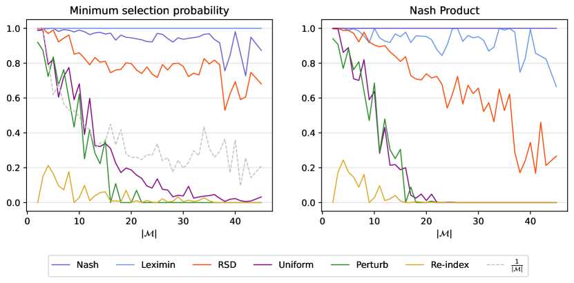
Figure 1: Average ratio of minimum selection probability (left) and Nash product (right) for agents in $\mathcal{M}$ compared to the optimum in kidney exchange instances, with respect to the number of agents in $\mathcal{M}$.

The leximin and the Nash distribution each outperform the other distributions on the criteria that they do not optimize, and perform close to the optimum. The RSD distribution obtains the third-highest performance on all criteria. Lastly, the uniform distribution, as well as the perturb and the re-index heuristics, all have ratios that are close to or equal to zero for larger instances. The minimum selection probability by the uniform distribution, for example, was less than 5% of the optimum in 30 out of the 50 instances with 70 patient-donor pairs, and for the perturb and re-index heuristics, the minimum was less than 5% in almost all instances of size 70. In comparison, the minimum selection probability by RSD is at least 40% of the optimum in all kidney exchange instances.

For reference, Figure 1 also shows how the ratio of $\frac{1}{|\mathcal{M}|}$ performs compared to the discussed rules, reflecting a situation in which all agents in $\mathcal{M}$ have an equal share of the decision power. We showed in Section 6 that the uniform rule violates the individual fair share property, and we can conclude from our computational experiments that this is not merely a theoretical result, but a common observation in practice.

Table 2 displays the required computational effort to find a partitioning of the agents, and to obtain each of the distributions. The computation time for finding an implementation of RSD is, as expected, very close to that of finding a single optimal solution, excluding the time to find a partitioning of the agents into $\mathcal{Y}$, $\mathcal{M}$, and $\mathcal{N}$. Combining this observation with the performance of RSD in Figure 1, this presents RSD-variants as a pragmatic method to control the selection probabilities of the optimal solutions. Furthermore, we can observe that the computation times for the leximin distribution scale better than for the Nash distribution in the kidney exchange instances.

Table 2: CPU time (in s) to find an optimal solution ($t_{\text{opt}}$), to find a partitioning of the agents into $\mathcal{Y}$, $\mathcal{M}$, and $\mathcal{N}$, and to compute the different distributions for the kidney exchange instances (KE). The asterisk-symbol (*) indicates that the distribution requires a prior partitioning of the agents, of which the time is not included.

inst	$\mathbf{t}_{\text{opt}}$	Partition	RSD*	Leximin*	Nash*	Uniform
KE10	0.002	0.007	0.002	0.004	0.060	0.003
KE20	0.006	0.059	0.006	0.054	0.137	1.678
KE30	0.010	0.161	0.010	0.159	0.251	15.105
KE40	0.014	0.301	0.016	0.446	0.578	47.775
KE50	0.019	0.469	0.027	0.769	0.967	77.588
KE60	0.021	0.714	0.038	2.147	3.301	83.760
KE70	0.030	1.046	0.064	2.518	14.425	115.546

9 Conclusion and future research directions

Following the observation that selecting one of the optimal solutions of an integer linear program in a deterministic way may result in an unfair treatment of the agents involved, we have introduced the fair integer programming problem, which studies how to control the selection probabilities of the optimal solutions of integer linear programs. We propose column generation frameworks to find distributions over the optimal solutions that optimize linear functions (e.g., maximizing the minimum selection probability of the agents), or that maximize concave functions (e.g., the Nash product of the agents’ selection probabilities). Moreover, we describe methods inspired by the Random Serial Dictatorship (RSD) mechanism that use a random ordering of the agents as a selection criterion. While we have developed our methods for integer linear programs with binary decision variables, which represent agents with dichotomous preferences, we discuss in Section 7 how our methods can be adapted to include the selection of near-optimal solutions, and to integer linear programs with real decision variables, which correspond to agents with cardinal preferences.

We have evaluated the proposed methods on the kidney exchange problem, and find that the Nash rule and the leximin rule outperform the proposed methods on the evaluated welfare criteria, followed by the RSD rule. Moreover, we show that the RSD distribution can be implemented through an intuitive algorithm in computation times that are similar to those of finding a single optimal solution. This result illustrates that addressing the fair integer programming problem does not necessarily cause an increase in the computational time for decision-makers and practitioners. Given the prevalence of integer programming formulations having multiple optimal solutions, we believe, therefore, that controlling the selection probabilities of the optimal solutions should be an essential step for decision-makers and practitioners who make high-impact decisions using integer programming techniques.

We identify three major directions for future research. First, our paper focuses on developing general-purpose algorithms that can be applied to a wide class of integer linear programs. The design of dedicated algorithms for specific problems that exploit the combinatorial structure of the problem at hand is an interesting research direction. Such specialized algorithms to compute the maximin distribition in polynomial time have been proposed, for example, by Li et al. (2014) for the kidney exchange problem, or by García-Soriano and Bonchi (2020) for cases where the optimal solutions form a matroid. Second, we suggest investigating the existence of alternative distributions other than RSD that can be implemented in computation times similar to those of finding a single optimal solution, possibly inspired by the wide range of solution concepts in the cooperative bargaining literature, or by introducing fairness considerations into the literature on symmetry breaking in integer programming. Lastly, we have focused on comparing the welfare performance of our column generation procedures to rules of which the underlying distributions could only be accurately computed by generating many optimal solutions (uniform, RSD, perturb, re-index). Therefore, we could only work with relatively small instances. A more extensive computational study of the column generation frameworks and of RSD implementations on larger instances and on other types of problems is a promising direction for future work.

Acknowledgements Tom Demeulemeester is funded by PhD fellowship 11J8721N of Research Foundation - Flanders. We would like to thank Markus Brill, Ágnes Cseh, and Jannik Matuschke for their valuable comments and suggestions.

Appendix A Proof of correctness column generation procedure Section 5.3

We adopt the same notation as in Section 5.3. Before proving the correctness of the column generation procedure described in Section 5.3, we point out that the following two conditions are satisfied. First, for any non-empty subset of the optimal solutions $\tilde{\mathcal{S}}$, convex program $[\mathcal{C}_{f}(\tilde{\mathcal{S}})]$ is clearly feasible. Second, for any convex function $f:\mathbb{R}^{n}\to\mathbb{R}$ and for any non-empty $\tilde{\mathcal{S}}\subseteq\mathcal{S}$, convex program $[\mathcal{C}_{f}(\tilde{\mathcal{S}})]$ satisfies strong duality. This follows from the observation that $[\mathcal{C}_{f}(\tilde{\mathcal{S}})]$ satisfies Slater’s condition (e.g., Boyd and Vandenberghe, 2004, Ch. 5.2.3) for any non-empty subset $\tilde{\mathcal{S}}\subseteq\mathcal{S}$, because its constraints are linear. As a result, the Karush-Kuhn-Tucker (KKT) conditions for a solution $(\bm{\lambda},\bm{d^{f}})$ of $[\mathcal{C}_{f}(\tilde{\mathcal{S}})]$ to be optimal over all solutions in $\tilde{\mathcal{S}}$ are both necessary and sufficient.

Given a solution $(\bm{\lambda^{*}},\bm{d^{*}})$ of $[\mathcal{C}_{f}(\tilde{\mathcal{S}})]$ with dual variables $\bm{\mu^{*}}$, $\rho^{*}$ and $\bm{\nu^{*}}$, the KKT conditions imply that $f$ is minimized over all optimal solutions in $\tilde{\mathcal{S}}\subseteq\mathcal{S}$ in point $(\bm{\lambda^{*}},\bm{d^{*}})$ if and only if the following conditions are satisfied:

Constraints $$(\ref{con:general_1})-(\ref{con:general_3}),$$

$$\nu^{*}_{s} \geq 0 \forall\;s=1,\ldots,|\tilde{\mathcal{S}}|,$$ (16a)

$$\nu^{*}_{s}\lambda^{*}_{s} =0 \forall\;s=1,\ldots,|\tilde{\mathcal{S}}|,$$ (16b)

$$\frac{\partial}{\partial d_{i}}f(\bm{d^{*}}) =\mu^{*}_{i} \forall\;i\in\mathcal{M},$$ (16c)

$$\sum_{i\in\mathcal{M}}\mu^{*}_{i}x^{s}_{i}+\rho^{*} =\nu^{*}_{s} \forall\;s=1,\ldots,|\tilde{\mathcal{S}}|.$$ (16d)

First, we show that the proposed column generation procedure terminates after a finite number of iterations. To do so, it suffices to show that the new solution $(\bm{x^{\prime}},\bm{y^{\prime}})$ that is found in each iteration $t$ was not yet in $\tilde{S}^{t}$. Starting from condition (16d), and by using the complementary slackness conditions (16b), the assumption that $\lambda^{*}_{old}>0$, and conditions (16b) that $\nu_{s}\geq 0$ for all solutions in $\tilde{\mathcal{S}}^{t}$, we obtain that

$$\sum_{i\in\mathcal{M}}\mu^{*}_{i}x^{old}_{i}=-\rho=\sum_{u\in\mathcal{M}}\mu^{*}_{i}x^{s}-\nu_{s}\leq\sum_{i\in\mathcal{M}}\mu^{*}_{i}x^{s}_{i},$$ (17)

for all solutions $(\bm{x^{s}},\bm{y^{s}})\in\tilde{\mathcal{S}}^{t}$. When condition (9) does not hold, this implies that $\sum_{i\in\mathcal{M}}\mu^{*}_{i}x^{\prime}_{i}<\sum_{i\in\mathcal{M}}\mu^{*}_{i}x^{old}_{i}\leq\sum_{i\in\mathcal{M}}\mu^{*}_{i}x^{s}_{i}$, for all solutions $(\bm{x^{s}},\bm{y^{s}})\in\tilde{\mathcal{S}}^{t}$, which shows that $(\bm{x^{\prime}},\bm{y^{\prime}})\notin{\tilde{S}^{t}}$.

Second, we show that condition (9) is indeed an optimality condition, and that a solution $(\bm{\lambda}^{*},\bm{d}^{*})$ of $[\mathcal{C}_{f}(\tilde{\mathcal{S}}^{t})]$ minimizes $f$ over all solutions in $\mathcal{S}$ if condition (9) holds. To show this, we will extend the variables $\bm{\lambda^{*}}$ and $\bm{\nu^{*}}$ to all solutions in $\mathcal{S}$. Let $\lambda^{*}_{s}$ and $\nu^{*}_{s}$ remain unchanged for solutions $(\bm{x^{s}},\bm{y^{s}})\in\tilde{\mathcal{S}}^{t}$, and let $\lambda^{*}_{r}=0$ and $\nu^{*}_{r}=\sum_{i\in\mathcal{M}}\mu^{*}_{i}x^{r}_{i}+\rho^{*}$ for all solutions $(\bm{x^{r}},\bm{y^{r}})\in\mathcal{S}\setminus\tilde{\mathcal{S}}^{t}$. Next, we show that if Condition (9) holds, $\bm{d^{*}}$, $\bm{\mu^{*}}$, $\rho^{*}$, and these extended variables $\bm{\lambda^{*}}$, and $\bm{\nu^{*}}$ satisfy the KKT conditions for $[\mathcal{C}_{f}(\mathcal{S})]$ over all solutions in $\mathcal{S}$, and will therefore minimize $f$ over $\mathcal{S}$.

Most of the conditions are directly implied by the fact that the KKT conditions hold for $[\mathcal{C}_{f}(\tilde{\mathcal{S}}^{t})]$, because all variables in the equations remain the same (Equation (16c) remains unchanged, and Equations (8d), (16a), (16b), and (16d) remain unchanged for all solutions $(\bm{x^{s}},\bm{y^{s}})\in\tilde{S}^{t}$). Clearly, the conditions imposed by Equations (8b) and (8c) are satisfied, because the newly introduced variables are equal to zero. Moreover, $\lambda_{s}=0$ for all $(\bm{x^{s}},\bm{y^{s}})\in\mathcal{S}\setminus\tilde{\mathcal{S}}^{t}$, which satisfies the conditions imposed by Equations (8d) and (16b). The conditions imposed by Equations (16a) are satisfied for all solutions $(\bm{x^{s}},\bm{y^{s}})\in\mathcal{S}\setminus\tilde{\mathcal{S}}^{t}$ by using our assumption that Condition (9) holds:

$$\sum_{i\in\mathcal{M}}\mu^{*}_{i}x^{s}_{i}\geq\sum_{i\in\mathcal{M}}\mu^{*}_{i}x^{\prime}_{i}\geq\sum_{i\in\mathcal{M}}\mu^{*}_{i}x^{old}_{i}\geq\sum_{i\in\mathcal{M}}\mu^{*}_{i}x^{old}_{i}-\nu^{*}_{old}=-\rho^{*}$$ (18)

By definition of $\nu^{*}_{s}$ for all solutions $(\bm{x^{s}},\bm{y^{s}})\in\mathcal{S}\setminus\tilde{\mathcal{S}}^{t}$, Equation (18) implies that $\nu_{s}^{*}\geq 0$. Lastly, the definition of the new $\nu^{*}_{s}$ implies that conditions (16d) hold.

References

- Abraham et al. (2007) Abraham, D.J., Blum, A., Sandholm, T., 2007. Clearing algorithms for barter exchange markets: Enabling nationwide kidney exchanges, in: Proceedings of the 8th ACM conference on Electronic commerce, pp. 295--304.
- Airiau et al. (2022) Airiau, S., Aziz, H., Caragiannis, I., Kruger, J., Lang, J., Peters, D., 2022. Portioning using ordinal preferences: Fairness and efficiency. Artificial Intelligence 314, 103809.
- Aziz et al. (2019) Aziz, H., Bogomolnaia, A., Moulin, H., 2019. Fair mixing: the case of dichotomous preferences, in: Proceedings of the 2019 ACM Conference on Economics and Computation, pp. 753--781.
- Aziz et al. (2013) Aziz, H., Brandt, F., Brill, M., 2013. The computational complexity of random serial dictatorship. Economics Letters 121, 341--345.
- Aziz and Mestre (2014) Aziz, H., Mestre, J., 2014. Parametrized algorithms for random serial dictatorship. Mathematical Social Sciences 72, 1--6.
- Bampis et al. (2018) Bampis, E., Escoffier, B., Mladenovic, S., 2018. Fair resource allocation over time, in: Proceedings of the 17th International Conference on Autonomous Agents and MultiAgent Systems, AAMAS ’18, pp. 766--773.
- Bertsimas et al. (2011) Bertsimas, D., Farias, V.F., Trichakis, N., 2011. The price of fairness. Operations Research 59, 17--31.
- Bogomolnaia and Moulin (2004) Bogomolnaia, A., Moulin, H., 2004. Random matching under dichotomous preferences. Econometrica 72, 257--279.
- Bogomolnaia et al. (2005) Bogomolnaia, A., Moulin, H., Stong, R., 2005. Collective choice under dichotomous preferences. Journal of Economic Theory 122, 165--184.
- Boyd and Vandenberghe (2004) Boyd, S., Vandenberghe, L., 2004. Convex Optimization. Cambridge university press.
- Brandl et al. (2021) Brandl, F., Brandt, F., Peters, D., Stricker, C., 2021. Distribution rules under dichotomous preferences: Two out of three ain’t bad, in: Proceedings of the 22nd ACM Conference on Economics and Computation, ACM-EC ’21, p. 158–179.
- Brandl et al. (2016) Brandl, F., Brandt, F., Seedig, H.G., 2016. Consistent probabilistic social choice. Econometrica 84, 1839--1880.
- Caragiannis et al. (2019) Caragiannis, I., Kurokawa, D., Moulin, H., Procaccia, A.D., Shah, N., Wang, J., 2019. The unreasonable fairness of maximum Nash welfare. ACM Transactions on Economics and Computation (TEAC) 7, 1--32.
- Carvalho and Lodi (2023) Carvalho, M., Lodi, A., 2023. A theoretical and computational equilibria analysis of a multi-player kidney exchange program. European Journal of Operational Research 305, 373--385.
- Chen and Hooker (2022) Chen, V.X., Hooker, J.N., 2022. Combining leximax fairness and efficiency in a mathematical programming model. European Journal of Operational Research 299, 235--248.
- Constantino et al. (2013) Constantino, M., Klimentova, X., Viana, A., Rais, A., 2013. New insights on integer-programming models for the kidney exchange problem. European Journal of Operational Research 231, 57--68.
- CPLEX (2021) CPLEX, 2021. Documentation/ILOG CPLEX Optimization Studio/12.9.0/Determinism of results. URL: https://www.ibm.com/docs/en/icos/12.9.0?topic=optimizers-determinism-results. accessed on 2023/06/12.
- Danna et al. (2007) Danna, E., Fenelon, M., Gu, Z., Wunderling, R., 2007. Generating multiple solutions for mixed integer programming problems, in: International Conference on Integer Programming and Combinatorial Optimization, Springer. pp. 280--294.
- Demeulemeester et al. (2023) Demeulemeester, T., Goossens, D., Hermans, B., Leus, R., 2023. A pessimist’s approach to one-sided matching. European Journal of Operational Research 305, 1087--1099.
- Dickerson et al. (2016) Dickerson, J.P., Manlove, D.F., Plaut, B., Sandholm, T., Trimble, J., 2016. Position-indexed formulations for kidney exchange, in: Proceedings of the 2016 ACM Conference on Economics and Computation, pp. 25--42.
- Dickerson et al. (2014) Dickerson, J.P., Procaccia, A.D., Sandholm, T., 2014. Price of fairness in kidney exchange, in: Proceedings of the 2014 International Conference on Autonomous Agents and Multi-Agent Systems, AAMAS ’14, p. 1013–1020.
- Duddy (2015) Duddy, C., 2015. Fair sharing under dichotomous preferences. Mathematical Social Sciences 73, 1--5.
- Elkind et al. (2022) Elkind, E., Kraiczy, S., Teh, N., 2022. Fairness in temporal slot assignment, in: Algorithmic Game Theory: 15th International Symposium, SAGT 2022, Springer. pp. 490--507.
- Farnadi et al. (2021) Farnadi, G., St-Arnaud, W., Babaki, B., Carvalho, M., 2021. Individual fairness in kidney exchange programs, in: Proceedings of the AAAI Conference on Artificial Intelligence, pp. 11496--11505.
- Fishburn (1984) Fishburn, P.C., 1984. Probabilistic social choice based on simple voting comparisons. The Review of Economic Studies 51, 683--692.
- Flanigan et al. (2021a) Flanigan, B., Gölz, P., Gupta, A., Hennig, B., Procaccia, A.D., 2021a. Fair algorithms for selecting citizens’ assemblies. Nature 596, 1--5.
- Flanigan et al. (2021b) Flanigan, B., Kehne, G., Procaccia, A.D., 2021b. Fair sortition made transparent. Advances in Neural Information Processing Systems 34, 25720--25731.
- García-Soriano and Bonchi (2020) García-Soriano, D., Bonchi, F., 2020. Fair-by-design matching. Data Mining and Knowledge Discovery 34, 1291--1335.
- Gibbard (1977) Gibbard, A., 1977. Manipulation of schemes that mix voting with chance. Econometrica 41, 665--681.
- Gurobi (2023) Gurobi, 2023. Is Gurobi deterministic? URL: https://support.gurobi.com/hc/en-us/articles/360031636051-Is-Gurobi-deterministic. accessed on 2023/06/12.
- Imai (1983) Imai, H., 1983. Individual monotonicity and lexicographic maxmin solution. Econometrica 51, 389--401.
- Kalai and Smorodinsky (1975) Kalai, E., Smorodinsky, M., 1975. Other solutions to Nash’s bargaining problem. Econometrica 43, 513--518.
- Karp (1972) Karp, R.M., 1972. Reducibility among combinatorial problems, in: Complexity of computer computations. Springer, pp. 85--103.
- Karsu and Morton (2015) Karsu, Ö., Morton, A., 2015. Inequity averse optimization in operational research. European Journal of Operational Research 245, 343--359.
- Lackner (2020) Lackner, M., 2020. Perpetual voting: Fairness in long-term decision making, in: Proceedings of the AAAI conference on artificial intelligence, pp. 2103--2110.
- Lawler and Moore (1969) Lawler, E.L., Moore, J.M., 1969. A functional equation and its application to resource allocation and sequencing problems. Management science 16, 77--84.
- Li et al. (2014) Li, J., Liu, Y., Huang, L., Tang, P., 2014. Egalitarian pairwise kidney exchange: fast algorithms via linear programming and parametric flow, in: Proceedings of the 13th International Conference on Autonomous Agents and MultiAgent Systems, AAMAS ’14, pp. 445--452.
- Lodi et al. (2022) Lodi, A., Olivier, P., Pesant, G., Sankaranarayanan, S., 2022. Fairness over time in dynamic resource allocation with an application in healthcare. Mathematical Programming (forthcoming).
- McElfresh and Dickerson (2018) McElfresh, D., Dickerson, J., 2018. Balancing lexicographic fairness and a utilitarian objective with application to kidney exchange, in: Proceedings of the AAAI Conference on Artificial Intelligence, pp. 1161--1168.
- Michorzewski et al. (2020) Michorzewski, M., Peters, D., Skowron, P., 2020. Price of fairness in budget division and probabilistic social choice, in: Proceedings of the AAAI conference on artificial intelligence, pp. 2184--2191.
- Murnighan et al. (1988) Murnighan, J.K., Roth, A.E., Schoumaker, F., 1988. Risk aversion in bargaining: An experimental study. Journal of Risk and Uncertainty 1, 101--124.
- Nash (1950) Nash, J.F., 1950. The bargaining problem. Econometrica 18, 155--162.
- Peters (2013) Peters, H.J., 2013. Axiomatic bargaining game theory. Springer Science & Business Media.
- Raiffa (1953) Raiffa, H., 1953. Arbitration schemes for generalized two-person games, in: Kuhn, H.W., Tucker, A.W. (Eds.), Contributions to the theory of games. Princeton University Press. volume 2. chapter 21, pp. 361--387.
- Roth (1979) Roth, A.E., 1979. Axiomatic models of bargaining. Lecture notes in economics and mathematical systems 170, Springer, Berlin.
- Roth and Malouf (1979) Roth, A.E., Malouf, M.W., 1979. Game-theoretic models and the role of information in bargaining. Psychological Review 86, 574.
- Roth et al. (1981) Roth, A.E., Malouf, M.W., Murnighan, J.K., 1981. Sociological versus strategic factors in bargaining. Journal of Economic Behavior & Organization 2, 153--177.
- Roth and Murnighan (1982) Roth, A.E., Murnighan, J.K., 1982. The role of information in bargaining: An experimental study. Econometrica 50, 1123--1142.
- Roth et al. (2005) Roth, A.E., Sönmez, T., Ünver, M.U., 2005. Pairwise kidney exchange. Journal of Economic Theory 125, 151--188.
- Roth et al. (2007) Roth, A.E., Sönmez, T., Ünver, M.U., 2007. Efficient kidney exchange: Coincidence of wants in markets with compatibility-based preferences. American Economic Review 97, 828--851.
- Saidman et al. (2006) Saidman, S.L., Roth, A.E., Sönmez, T., Ünver, M.U., Delmonico, F.L., 2006. Increasing the opportunity of live kidney donation by matching for two-and three-way exchanges. Transplantation 81, 773--782.
- Serra and Hooker (2020) Serra, T., Hooker, J.N., 2020. Compact representation of near-optimal integer programming solutions. Mathematical Programming 182, 199--232.
- St-Arnaud et al. (2022) St-Arnaud, W., Carvalho, M., Farnadi, G., 2022. Adaptation, comparison and practical implementation of fairness schemes in kidney exchange programs. arXiv:2207.00241 .
- Thomson (1994) Thomson, W., 1994. Cooperative models of bargaining. Handbook of game theory with economic applications 2, 1237--1284.
- Thomson (2022) Thomson, W., 2022. On the axiomatic theory of bargaining: a survey of recent results. Review of Economic Design 26, 1--52.
- Valiant (1979a) Valiant, L.G., 1979a. The complexity of computing the permanent. Theoretical Computer Science 8, 189--201.
- Valiant (1979b) Valiant, L.G., 1979b. The complexity of enumeration and reliability problems. SIAM Journal on Computing 8, 410--421.
- Vempala (2005) Vempala, S., 2005. Geometric random walks: a survey. Combinatorial and Computational Geometry 52, 573--612.