OptMSM: Optimizing Multi-Scenario Modeling for Click-Through Rate Prediction

Abstract

A large-scale industrial recommendation platform typically consists of multiple associated scenarios, requiring a unified click-through rate (CTR) prediction model to serve them simultaneously. Existing approaches for multi-scenario CTR prediction generally consist of two main modules: i) a scenario-aware learning module that learns a set of multi-functional representations with scenario-shared and scenario-specific information from input features, and ii) a scenario-specific prediction module that serves each scenario based on these representations. However, most of these approaches primarily focus on improving the former module and neglect the latter module. This can result in challenges such as increased model parameter size, training difficulty, and performance bottlenecks for each scenario. To address these issues, we propose a novel framework called OptMSM (Optimizing Multi-Scenario Modeling). First, we introduce a simplified yet effective scenario-enhanced learning module to alleviate the aforementioned challenges. Specifically, we partition the input features into scenario-specific and scenario-shared features, which are mapped to specific information embedding encodings and a set of shared information embeddings, respectively. By imposing an orthogonality constraint on the shared information embeddings to facilitate the disentanglement of shared information corresponding to each scenario, we combine them with the specific information embeddings to obtain multi-functional representations. Second, we introduce a scenario-specific hypernetwork in the scenario-specific prediction module to capture interactions within each scenario more effectively, thereby alleviating the performance bottlenecks. Finally, we conduct extensive offline experiments and an online A/B test to demonstrate the effectiveness of OptMSM.

1 Introduction

Click-through rate (CTR) prediction is a crucial component in online recommendation platform [5, 19, 3, 23], which aims to predict the probability of candidate items being clicked and return top-ranked items for each user. In practice, a business is usually divided into different scenarios based on different user groups or item categories [4, 6, 20], and the resource overhead of customizing a proprietary CTR prediction model for each scenario is too high. Therefore, designing and deploying a unified CTR prediction model to efficiently serve all scenarios is a realistic challenge for a large-scale industrial recommendation platform. Taking the Tencent Licaitong financial recommendation platform used in the online experiment as an example, as shown in Fig. 1, these scenarios include the homepage (HP), balanced investment portfolio page (BIP), and aggressive investment portfolio page (AIP). Specifically, HP is the first page that each user interacts with, where the users usually browse the items without specific intent. The categories of items are mixed. The BIP and AIP pages list the items with corresponding categories for the users with different specific intents, respectively. We focus on how to effectively utilize all the user interactions in multiple scenarios to obtain a desired CTR prediction model.

(a) Homepage

(b) BIP page

(c) AIP page

Figure 1: The scenarios in Tencent Licaitong financial recommendation platform.

Different from single-scenario modeling [35], multi-scenario modeling (MSM) for CTR prediction is proposed in previous works to address the above goals. Existing works for MSM usually adopt the idea of multi-task learning to model the relationship between different scenarios [36, 17, 26]. They usually contain two main modules, i.e., the scenario-aware learning module and the scenario-specific prediction module. The former is used to learn versatile scenario-aware representations, where scenario-shared and scenario-specific information are captured simultaneously. The latter uses a scenario-specific architecture to predict the corresponding scenario based on scenario-aware representations. Obviously, the scenario-aware learning module carries more learning burden during training, and most of the existing works focus on improving the effectiveness of this module in modelling the multi-functional representations, where increasingly complex architectures are proposed [13, 25, 34, 31, 11, 37, 2]. Although these works have shown promising results, these complex architectures also increase both the model complexity and the training cost, which becomes an obstacle to generalization to more business scenarios. On the other hand, improvements for scenario-specific prediction modules are usually neglected in previous works, i.e., they only utilize simple fully-connected layers as the architecture of the predictor, which may lead to performance bottlenecks within each scenario.

In this paper, to address the above problems, we propose a novel Optimizing Multi-Scenario Modelling (OptMSM) framework. We propose a novel scenario-enhanced learning module to alleviate the first problem. Specifically, we incorporate scenario priors to partition the input feature set into scenario-specific and scenario-shared features, mapped to an embedding encoding specific information and a set of embeddings encoding shared information. After introducing adaptive gating and orthogonality constraints on the latter to facilitate the separation of shared information corresponding to each scene, it is combined with the former to obtain the multifunctional representation. Since neither adaptive gating nor orthogonality constraints require additional learnable parameters, and the separate modelling of feature sets eases the learning burden, the scenario-enhanced learning module provides an effective and efficient way to obtain the desired representations. Inspired by the effectiveness of feature interactions in single-scenario modelling, we then develop a scenario-specific hypernetwork to deal with the second problem, which generates adaptive network parameters based on scenario-aware representations. In this way, scenario-aware representations can fully interact with scenario-specific predictors to further improve performance. Moreover, as shown in Section 4.2, our framework can also be effectively integrated with existing multi-scenario models to improve performance.

2 Related Work

In this section, we briefly review some related works on two topics, including single-scenario modelling and multi-scenario modelling for CTR prediction.

Single-Scenario Modeling for CTR Prediction. Traditional CTR prediction aims to leverage the user interactions within a specific scenario to train an effective model for this scenario [22, 5, 19, 16]. Most existing works on this topic focus on improving the modelling of feature interactions to enhance the performance of models, and many representative methods have been proposed. For example, DeepFM combines factorization machine and deep network layer to model the feature interactions [8], DCN [29] and DCN-V2 [30] develop a novel cross-network layer to further characterize the explicit feature interactions, and APG [33] proposes an adaptive parameter generation network for deep CTR prediction models, which can enhance the representation of feature interactions per instance with a larger parameter space. In addition, some recent works have introduced various automated machine learning ideas to efficiently find a suitable feature interaction architecture, such as AutoFIS [14] and OptInter [15]. Overall, previous works have shown that the design of feature interaction architecture is an important factor in improving the performance of single-domain CTR models, which is neglected in multi-scenario modelling for CTR prediction.

Multi-Scenario Modeling for CTR Prediction. Multi-scenario CTR modelling aims to leverage all the user interactions in different scenarios to train one or more models to serve these scenarios simultaneously [13, 24, 11, 25, 31, 37, 7], where the key question is how to use shared-specific information to learn the versatile scenario-aware representations, and then use a scenario-specific architecture for per-scenario prediction. A lot of work has been proposed to improve the effectiveness of scenario-aware representation learning. For example, STAR [25] designs a novel topological dependency to fully exploit the relationship between different scenarios. SAR-Net [24] introduces a scenario-aware attention module to extract scenario-specific user features, and a corresponding gating mechanism is designed to fuse them with shared information. CausalInt [31] introduces the priors on causal graphs to efficiently extract shared information and reduce negative transfer. However, these methods will significantly increase the model parameter size and training difficulty. Furthermore, ignoring the improvement of scenario-specific predictor architectures will lead to performance bottlenecks.

3 Preliminary

In this section, we first give a formal definition of the multi-scenario CTR prediction task. Given a set of scenarios $S=\{s^{m}\}^{M}_{m=1}$ and a set of training instance $\{(\mathbf{x},y,s^{m})\}^{N}_{n=1}$, where $\mathbf{x}\in\mathbf{X}$ is the feature vector, $y\in\{0,1\}$ is the label, and $m\in\{1,\cdots,M\}$ is the scenario indicator corresponding to each instance. The multi-scenario CTR prediction task needs to perform CTR prediction on these $M$ related scenarios,

$$\hat{y}=\mathcal{F}(\mathbf{x},y,s^{m}),$$ (1)

where $\mathcal{F}$ is the multi-scenarios model and $\hat{y}$ is the predicted label. Further, we can decompose this task into two stages, i.e., scenario-aware representation learning $f(\cdot)$ and scenario-specific prediction $g(\cdot)$,

$$\mathcal{R}^{s^{m}}=f(\mathbf{x},s^{m}\mid\mathbf{W}),$$ (2)

$$\hat{y}=g(\mathcal{R}^{s^{m}}\mid\{\mathbf{W}^{s^{m}}\}),$$

where $\mathbf{W}$ and $\{\mathbf{W}^{s^{m}}$} are weight parameters of the two stages, respectively. Therefore, the optimization objective for multi-scenario CTR prediction can be formalized as,

$$\mathcal{L}_{msm}=\sum_{n=1}^{N}\ell(y_{n},\hat{y}_{n}),$$ (3)

where $\ell$ is an arbitrary loss function, such as a cross-entropy loss.

4 The Proposed Framework

The proposed framework for optimizing multi-scenario modelling, or OptMSM for short, is shown in Fig. 2. The OptMSM consists of three steps. First, the input feature partition module incorporates the scenario priors to partition the input features. Then, the scenario-enhanced learning module models the disentangled representation corresponding to each scenario from the scenario-shared features. Finally, after combining scenario-specific information and disentangled representation, a scenario-aware representation interaction module is used to explore the interactions within each scenario to enhance predictive performance. We will describe each module in detail based on the training process.

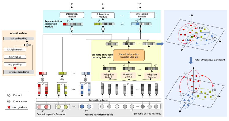
Figure 2: The architecture of our OptMSM framework.

4.1 The Input Features Partition Module

To ease the model’s learning burden for scenario-aware representations, we propose to divide the input features into two groups and model them separately, including scenario-specific features $\mathbf{x}^{m}$ and scenario-shared features $\mathbf{x}_{c}$, i.e. $\mathbf{x}=\{\mathbf{x}^{m},\mathbf{x}_{c}\}$. An example of different categories of input features is listed in Table 1. It can be observed that some features are specific to certain scenarios, such as scenario id, while others are shared among all scenarios, such as gender. Note that previous modelling paradigms do not differentiate input feature categories. Therefore, scenario-specific features are difficult to transfer across scenarios during learning scenario-aware representations, and scenario information is hard to capture in the final prediction. Hence, the intuitive motivation for this module is to resolve these issues. In addition, the model needs more effort to reasonably balance the modeling of two categories of features. Next, we transform scenario-specific and scenario-shared features into corresponding low-dimensional embeddings and feed them into the following modules for further modeling.

$$\begin{gathered}\mathbf{e}^{m}=\mathbf{E}^{m}(\mathbf{x}^{m})\quad\&\quad\mathbf{e}_{c}=\mathbf{E}(\mathbf{x}_{c}),\end{gathered}$$ (4)

where $\mathbf{E}^{m}$, $\mathbf{e}^{m}$, $\mathbf{E}$, $\mathbf{e}_{c}$ are the embedding tables and embeddings corresponding to the two category features, respectively.

Table 1: An example of features included in the online financial recommendation platform used in the experiments.

Feature Category	Example
User Common Features	gender,age, user behaviors, etc.
Item Common Features	item category, item price, etc.
Context Common Features	time, market condition
User Scenario-specific Features	user behaviors in scenarios
Item Scenario-specific Features	item statistics, item appearance in scenarios, etc.
Context Scenario-specific Features	scenario id, item position in scenarios, etc.

4.2 The Scenario Enhanced Learning Module

After receiving the scenario-shared feature embeddings $\mathbf{e}_{c}$ generated by the previous module, we need to leverage cross-scenario information sharing and transfer to learn effective scenario-aware representations for different scenarios. An intuitive idea is that each scenario should pay extra attention to scenario-shared features [11]. Therefore, we first introduce an adaptation gate for each scenario to refine $\mathbf{e}_{c}$ with scenario-specific information. In this paper, we take Squeeze-and-Excitation (SE-Net) [10] as an example implementation,

$$\begin{gathered}\mathbf{z}^{m}=\sigma(W^{m}[average(\mathbf{e}_{c1}),...,average(\mathbf{e}_{ci})]+b^{m}),\\ \mathbf{e}_{c}^{m}=concat([z_{1}^{m}*\mathbf{e}_{c1},...,z_{i}^{m}*\mathbf{e}_{ci}]),\end{gathered}$$ (5)

where $\mathbf{z}^{m}=\left(z_{1}^{m},z_{2}^{m},\cdots,z_{i}^{m}\right)$ is the refined weight vector for scenario $m$, $W^{m}$ and $b^{m}$ are the corresponding learnable parameters, and $i$ is the number of scenario-shared features. Note that adaptive gates can be implemented differently, such as an attention layer [27] or a perceptual layer [24], and the SE-Net block will be a lightweight approach for our purposes. Next, a built-in shared information transfer module aims to utilize the information synergy among all the scenarios to further distinguish different concerns of different scenarios on scenario-shared information. The issues for this module focus on how to transfer and what to transfer.

How to Transfer. A range of scenario-aware learning architectures have been explored in previous works on multi-scenario modeling, and they are easily integrated into this module. Here are some examples to illustrate the process:

• shared network: The shared network aims to extract commonality from all the scenarios and can be expressed as follows,

  $$r_{shared}=\mathbf{MLP}_{shared}(\mathbf{e}_{c}^{m}),$$ (6)

  where $\mathbf{MLP}_{shared}$ is the multilayer perception network shared by all the scenarios. Note that multiple similar $\mathbf{MLP}_{shared}$ are used in MMOE, the parameters of $\mathbf{MLP}_{shared}$ are shared without explicit output in STAR, and the output of multiple $\mathbf{MLP}_{shared}$ are used as a shared expert component in PLE.

• scenario-specific network: The scenario-specific network aims to squeeze out scenario-specific information from shared information, in which only scenario-specific data are used,

  $$r_{scenario}^{m}=\mathbf{MLP}^{m}(\mathbf{e}_{c}^{m}),$$ (7)

  where $\mathbf{MLP}^{m}$ is the scenario-specific network. Note that the number of $\mathbf{MLP}^{m}$ can be set according to the plugged module, e.g., 0 in MMOE, equal to the number of scenarios in STAR, and a predefined value in PLE.

• transferring layer: In some previous works, different methods are introduced to jointly model the above two networks. For example, STAR proposes the FCN topology dependence, and PLE introduces the gated network. To illustrate the transfer process, we use FCN as an example,

  $$r_{transfer}^{m}=FCN(\mathbf{e}_{c}^{m})=(W_{shared}\otimes W^{m})\cdot\mathbf{e}_{c}^{m}+b_{shared}+b^{m},$$ (8)

  where $\{W_{shared},b_{shared}\}$ and $\{W^{m},b^{m}\}$ are parameters in $\mathbf{MLP}_{shared}$ and $\mathbf{MLP}^{m}$, respectively, and $\otimes$ denotes element-wise multiplication.

Finally, this module will generate representations for all the scenarios, denoted as $\{r^{m}\mid m\in[1,M]\}$.

What to Transfer. Note that the scenario-aware representations are learned based on the model that mixes samples from all the scenarios. As a result, negative transfer often occurs, which perturbs the scenario-aware representations and misleads subsequent top-level predictions. A critical issue to mitigate the negative transfer effect is disentangling the representations between different scenarios. Inspired by the disentangled representation learning [21], we propose an explicit orthogonality constraint on the representation obtained above as an auxiliary loss to achieve this goal. Note that the number of samples in all the scenarios is usually unbalanced, and it is difficult to deal with the constraints of cross-sample representations. Therefore, we propose a strategy for enhanced learning. More specifically, for a sample $b$, we generate its representations in all the scenarios, i.e., $\{r_{b}^{1},\cdots,r_{b}^{m}\}$. Only one representation corresponding to the real scenario will be used for prediction in subsequent layers, while the others are used as contrastive representations to compute the orthogonality constraint. Orthogonal constraints will make these representations perpendicular to each other to ensure independence and successfully disentangle scenario-specific information. Note that the idea behind this strategy is similar to contrastive loss [28]. Formally, the loss can be expressed as follows,

$$\mathcal{L}_{orth}=\sum_{\begin{subarray}{c}i\neq j\\ b\in B\end{subarray}}<r_{b}^{i},r_{b}^{j}>\text{,}\quad<r_{b}^{i},r_{b}^{j}>=\frac{r_{b}^{i}\cdot r_{b}^{j}}{\Arrowvert r_{b}^{i}\Arrowvert_{2}\cdot\Arrowvert r_{b}^{j}\Arrowvert_{2}}$$ (9)

where $\Arrowvert\cdot\Arrowvert_{2}$ refers to the $\mathit{l}_{2}$ norm, and $B$ is the size of the mini-batch. Note that although the loss is conducted on $C_{m}^{2}$ pairs, it can be efficiently implemented in a vectorized manner at the mini-batch level and avoids loops.

4.3 The Scenario-Aware Representation Interaction Module

Although we get the disentangled scenario-aware representation, we still need to augment the representation with prior scenario-specific features in Eq.(4). On the one hand, scenario-specific information has a solid induction to the corresponding scenario, which helps the final prediction. On the other hand, considering complex interactions has been shown to benefit the performance of single-scenario CTR modeling. Therefore, to give the prediction more perception of prior information, we design a hypernetwork adaptively generating scenario-aware parameters [2, 9], which provides a full representation interaction. We give a detailed illustration of this module as shown in Fig. 3.

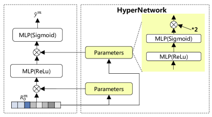
Figure 3: The scenario-aware hypernetwork for parameters generation.

To preserve the priors, we only concatenate the prior scenario-specific features embeddings $\mathbf{e}^{m}$ with disentangled scenario-aware representation $r^{m}$,

$$\mathcal{R}_{0}^{m}=r^{m}\oplus\mathbf{e}^{m}.$$ (10)

We then adopt a two-layer perception to generate parameters from the representations, i.e.,

$$\begin{gathered}\mathbf{\mathbb{R}}_{0l}=Relu(w_{0}\mathcal{R}_{0}^{m}+b_{0}),\\ \mathbf{\mathbb{R}}_{1l}=2\star\sigma(w_{1}\mathbf{\mathbb{R}}_{0l}+b_{1}),\end{gathered}$$ (11)

where $\sigma$ is sigmoid function, $\mathbf{\mathbb{R}}_{1l}$ has the same shape as $\mathcal{R}_{l}^{m}$, and $l$ is is the current layer number. Setting the coefficient to 2 in Eq.(11) is to scale the mean of sigmoid output to 1. After parameters are generated, we interact $\mathbf{\mathbb{R}}_{1l}$ with each layer in each scenario-specific predictor,

$$\mathcal{R}_{l}^{m}=\mathcal{R}_{l}^{m}\otimes\mathbf{\mathbb{R}}_{1l},\ l\in\{0,\cdots,L-1\}$$ (12)

where $\mathcal{R}_{l}^{m}$ is the latent output of layer $l$ in the scenario $m$, and $L-1$ is the number of layers in each scenario. Finally, the final score for $m$-th scenario can be get,

$$\hat{y}^{m}=\sigma(W_{L-1}R_{L-1}^{m}+b_{L-1}),$$ (13)

where $W_{n-1},b_{n-1}$ is the parameters of classifier. After combining Eq.(3), (9) and (13), We can get the final optimization objective,

$$\mathcal{L}=\mathcal{L}_{msm}+\lambda\cdot\mathcal{L}_{orth},$$ (14)

where $\lambda$ is a hyper-parameter controlling the orthogonality constraint.

5 Experiments

In this section, we conduct comprehensive experiments with the aim of answering the following five key questions.

• RQ1: Could OptMSM achieve superior performance compared with mainstream multi-scenario models?

• RQ2: Could OptMSM transfer to more multi-scenario models?

• RQ3: How does each module of OptMSM contribute to the final results?

• RQ4: Does OptMSM really get the optimal scenario-aware representation?

• RQ5: How does OptMSM perform in real-world recommendation scenarios?

5.1 Experiment Setup

Datasets. We conduct our offline experiments on three datasets, including two publicly multi-scene CTR benchmark datasets (Ali-CCP and AliExpress) and a private product dataset. Ali-CCP is collected from the traffic log of Tabao, and we divide logs into three scenarios according to the scenario id. AliExpress is collected from the AliExpress search system, which contains user behaviours from five countries. We consider each country as an advertising scenario and select four countries in our experiments following the setting of previous work [38]. The real product dataset comes from the financial business scenario of Tencent Licaitong, and we collect consecutive 4 weeks of user feedback logs from four scenarios, respectively. For Ali-CCP, following previous work [32], we use all the single-valued categorical features and take 10% of the train set as the validation set to verify models. For AliExpress, we split the training set and test set according to the settings in the original paper [13]. For the production dataset, we keep data on the last day as the test set, and the rest as the training and validation sets. Table 2 summarize the statistics for these datasets. We can observe that the data distribution in Ali-CCP and Production is obviously unbalanced.

Table 2: Statistics of datasets used in offline experiments. For impression and click, the percentages in each scenario are given in brackets.

Dataset	#Scenarios	#Impression	#Click
Ali-CCP	3	85,316,519 (0.75/37.79/61.46)	3,317,703 (0.84/38.91/60.25)
AliExpress	4	103,814,836 (17.07/26.04/30.51/26.38)	2,215,494 (17.02/24.49/38.15/20.34)
Production	4	823,972,400 (68.96/3.93/8.05/19.06)	59,466,088 (47.38/7.21/14.09/31.32))

Comparison Models. To verify the effectiveness of our proposed framework, we compare OptMSM with the following models. Mix: The model with a 3-layer fully-connected network is trained with a mixture of samples from all Scenarios; S-B: We share the embedding table across scenarios, and each scenario-specific network is the same as Mix, i.e., shared bottom model; MMoE [17]: We adopt a shared Mixture-of-Experts model, where each expert is a 3-layer fully-connected network and the number of experts equals $2*\#scenarios$; HMOE [13]: Except for explicit relatedness in the label space introduced by HMOE, the other settings are the same as MMOE; PLE [26]: The core module of PLE is CGC (Customized Gate Control), which consists of scenario-specific experts and shared experts. We keep the number of the former the same as MMOE with two additional shared experts; STAR [25]: This model consists of a centered network shared by all scenarios and the scenario-specific network for each scenario. The architectures of all networks are the same as Mix; and PEPNet [2]: This model adopts personalized prior information to enhance embedding and parameter personalization, and only has scenario-specific towers for predictions.

Implementation Details & Evaluation Settings. All models are implemented on Tensorflow [1] and trained with Adam optimizer [12]. We tune learning rate from [$10^{-2}$, $10^{-3}$, $10^{-4}$, $10^{-5}$], L2 weight from [$10^{-3}$, $10^{-4}$, $10^{-5}$, $10^{-6}$], and dropout rate from [0.1, 0.2, 0.3, 0.4]. The batch sizes for each dataset are set as 2048, 2048, and 512, respectively. The embedding dimensions are set as 20, 10, and 10. Besides, the hidden layers of the fully connected network are fixed to [256, 128, 32]. Following the previous works [8, 25], we use two common metrics in CTR prediction, i.e., AUC (Area Under ROC) and Logloss (based on cross-entropy).

5.2 RQ1: Overall Performance

We show the overall performance of our OptMSM and other baselines in Table 3. We summarize our observations below: 1) OptMSM generally outperforms baselines in most scenarios in three datasets. Specifically, OptMSM performs consistently well in three scenarios in the Ali-CCP dataset and improves significantly in the first sparse scenario. In the other two datasets, our OptMSM performs better in most scenarios to different degrees. Although OptMSM achieves the second performance in some scenarios, note that the difference is within 0.1%, which is also acceptable considering OptMSM gains statistical improvements in other scenarios; 2) On the whole, MSM can boost performance in all scenarios compared with the model trained with mixed data. However, this model performs slightly better than others in scenarios with sparse training samples. For example, the Mix model performs better in Ali-CCP S1 and Production S2. The possible reason for this is that samples in other scenarios are far more than these two scenarios and can directly help prediction in these two scenarios; and 3) PEPNet performs consistently better in AliExpress compared with other baselines while achieving relatively poor performance in other skewed datasets. Note that the distribution of AliExpress is more balanced than the other two datasets. Hence, this comparison directly verifies the effectiveness of information priors in some datasets and indirectly reflects that positive transfer is important when spares scenarios exist.

Table 3: The overall performance over three datasets. The boldface and underline indicate the highest score of all the models and baselines. $\star$ indicates significant level p-value $<0.05$.

	Scenario	Metric	Mix	S-B	MMOE	HMOE	PLE	STAR	PepNet	OptMSM
Ali-CCP	S1	AUC	0.5921	0.5899	0.5955	0.5979	0.5943	0.5924	0.5941	$\mathbf{0.6023}^{\star}$
		Logloss	0.1838	0.1855	0.1811	0.1801	0.1811	0.1906	0.1922	$\mathbf{0.1782}^{\star}$
	S2	AUC	0.6166	0.6202	0.6183	0.6214	0.6198	0.6246	0.6203	$\mathbf{0.6257}^{\star}$
		Logloss	0.1673	0.1663	0.1657	0.1662	0.1657	0.1715	0.1724	$\mathbf{0.1648}^{\star}$
	S3	AUC	0.6141	0.6164	0.6151	0.6183	0.6165	0.6175	0.6168	$\mathbf{0.6231}^{\star}$
		Logloss	0.1641	0.1600	0.1596	0.1601	0.1596	0.1601	0.1693	$\mathbf{0.1587}^{\star}$
AliExpress	NL	AUC	0.7256	0.7253	0.7257	0.7261	0.7256	0.7257	0.7258	$\mathbf{0.7286}^{\star}$
		Logloss	0.1087	0.1086	0.1081	0.1080	0.1079	0.1084	0.1078	$\mathbf{0.1077}$
	FR	AUC	0.7247	0.7256	0.7258	0.7260	0.7263	0.7258	$\mathbf{0.7266}$	0.7256
		Logloss	0.1010	0.1013	0.1009	0.1007	0.1008	0.1009	0.1006	$\mathbf{0.1004}$
	ES	AUC	0.7272	0.7276	0.7281	0.7285	0.7279	0.7277	0.7290	$\mathbf{0.7301}^{\star}$
		Logloss	0.1211	0.1210	0.1207	0.1207	0.1208	0.1211	0.1204	$\mathbf{0.1201}$
	US	AUC	0.7084	0.7059	0.7082	0.7084	0.7084	0.7073	0.7088	$\mathbf{0.7108}^{\star}$
		Logloss	0.1015	0.1008	0.1008	0.1006	0.1006	0.1007	$\mathbf{0.1004}$	0.1005
Production	S1	AUC	0.8718	0.8853	0.8866	0.8811	0.8872	0.8875	0.8866	$\mathbf{0.8890}^{\star}$
		Logloss	0.0951	0.0914	0.0954	0.0982	0.0958	0.0862	0.0956	$\mathbf{0.0848}^{\star}$
	S2	AUC	0.8997	0.9065	0.9069	0.9004	$\mathbf{\underline{0.9077}}$	0.9069	0.9068	0.9071
		Logloss	$\mathbf{0.0246}$	0.0248	0.0256	0.0259	0.0258	0.0259	0.0317	0.0247
	S3	AUC	0.8414	0.8478	0.8491	0.8502	0.8496	0.8515	0.8507	$\mathbf{0.8524}^{\star}$
		Logloss	0.0361	0.0288	0.0286	0.0286	0.0288	0.0276	0.0340	$\mathbf{0.0273}$
	S4	AUC	0.8665	0.8765	0.8759	0.8774	0.8768	0.8756	0.8773	$\mathbf{0.8808}^{\star}$
		Logloss	0.0569	0.0584	0.0581	0.0586	0.0585	0.0575	0.0654	$\mathbf{0.0538}^{\star}$

5.3 RQ2: Transferability Analysis

In this subsection, we investigate the transferability of our framework. We introduce FCN as our shared information transfer module in our framework. Here we extend our framework to other operation modules to illustrate whether our framework really optimizes the key factors for these modules. As shown in Fig. 4, we extend our OptMSM with transfer operations, including FCN, MoE, and CGC. Compared with the corresponding model, OptMSM improves its performance in all the scenarios, further validating the effectiveness of our design optimizing module. To investigate whether the additional optimization will bring a lot of computation cost, we report the training time of these models in Table 4. Notably, the increment of training time of OptMSM is acceptable.

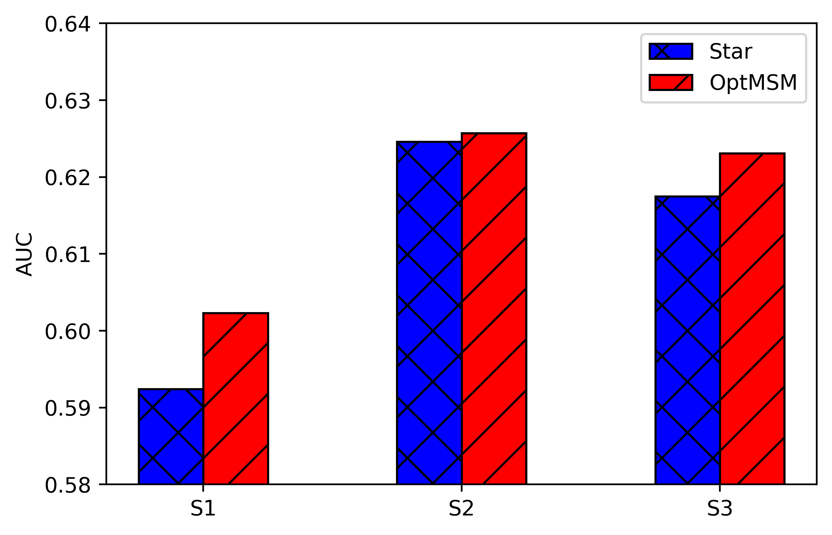
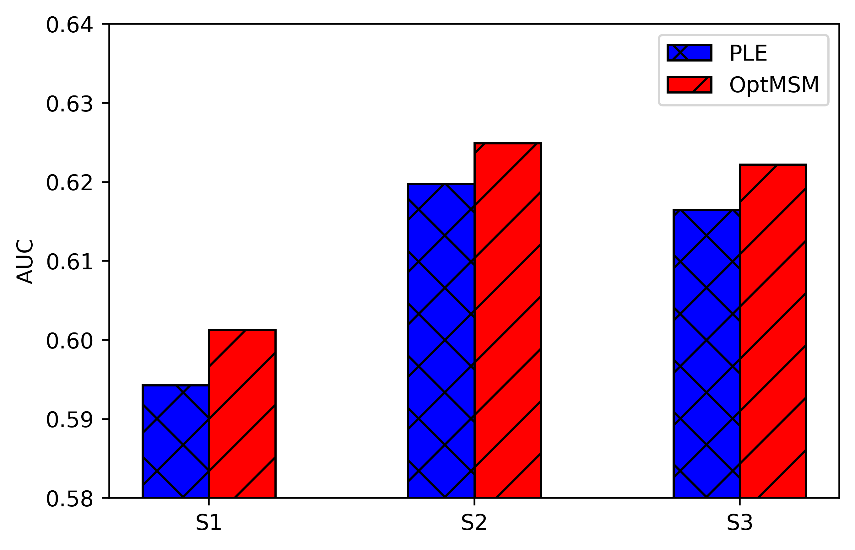
Figure 4: Transferable analysis of OptMSM with different operation on Ali-CCP.

Table 4: Training cost comparison on the Ali-CCP.

Model	Star	OptMSM(FCN)	MMoE	OptMSM(MoE)	PLE	OptMSM(CGC)
Cost (s)	684	716 (+4.68%)	692	724 (+4.62%)	941	982 (+4.36%)

5.4 RQ3&RQ4: Ablation Study

In this subsection, we validate the contribution of each component of OptMSM. We conduct a series of ablation studies over the datasets by examining the AUC after removing each component. The results are summarized in Table 5 and 6. The observations are summarized as follows: (1) All three components play important roles in optimizing different architectures, proving our optimizing framework’s effectiveness. (2) In both datasets, removing orthogonal constraints generally suffers from the most decrement in AUC, which means the disentangled representation is effective. (3)Because of the significant improvement of PEPNet in AliExpress, removing hypernetwork in AliExpress is harmful to our framework, which indicates that our framework optimizing scenario-specific prediction module is useful. As the disentangled representation is a key factor in our OptMSM, we further illustrate visual results by comparing the t-SNE [18] representations with and without orthogonal constraint in Fig. 5. Note that our constraint is effective in explicitly disentangling representation.

Table 5: Ablation study on OptMSM with FCN for Ali-CCP. w/o means removing the corresponding component, and the relative decrement is reported in the brackets.

Model	S1	S2	S3
OptMSM	0.6023	0.6257	0.6231
w/o priors	0.6014 (-0.15%)	0.6247 (-0.16%)	0.6222 (-0.14%)
w/o constraint	0.6010 (-0.22%)	0.6246 (-0.18%)	0.6219 (-0.19%)
w/o hypernetwork	0.6016 (-0.12%)	0.6249 (-0.13)	0.6223 (-0.13%)

Table 6: Ablation study on OptMSM with CGC for AliExpress. w/o means removing the corresponding component, and the relative decrement is reported in the brackets.

Model	NL	FR	ES	US
OptMSM	0.7290	0.7268	0.7312	0.7117
w/o priors	0.7288 (-0.03%)	0.7260 (-0.11%)	0.7302 (-0.14%)	0.7112 (-0.07%)
w/o constraint	0.7277 (-0.18%)	0.7263 (-0.07%)	0.7301 (-0.15%)	0.7108 (-0.13%)
w/o hypernetwork	0.7280 (-0.14%)	0.7265 (-0.04)	0.7302 (-0.14%)	0.7107 (-0.14%)

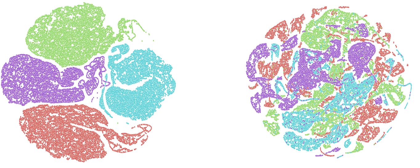
Figure 5: Visualization results on the representation in AliExpress. Left: with orthogonal constraint; Right: without orthogonal constraint.

5.5 RQ5: Online Experiments

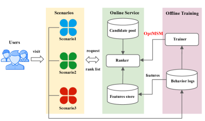
Figure 6: Overview of the financial product recommender system.

In this subsection, we report the online experiment results of our OptMSM in a financial product recommender system for four consecutive weeks, and the results further verify the effectiveness of our OptMSM. Firstly, we briefly present the recommender system overview, shown in Fig. 6. This system has two main components: Online Service and Offline Training respectively. When users access any scenarios, a rank list request will be sent to the online service. Meanwhile, the user’s attributes and contextual features will also be sent to the ranker, which utilizes the offline model to predict the score. In offline training, the ranker leverages behaviour historical logs, and the trainer trains the model based on the logs daily. Our OptMSM trains a unified model here to serve multiple scenarios. We deploy the OptMSM on four scenarios in this financial product recommender platform, which serves millions of daily active users. And the model is trained in a single cluster, where each node contains 96-core Intel(R) Platinum 8255C CPU, 256GB RAM, and 8 NVIDIA TESLA A100 GPU cards. Besides using Click Through Rate (CTR)(i.e. $\frac{\#click}{\#impression}$), a commonly-used online evaluation metric, we also use purchase amount per mille (PAPM), defined as $\frac{\#purchase\_amount}{\#impression}\times 1000$. Briefly, our OptMSM improve the overall performance, achieving +1.42%, +1.76%, +1.26% and +0.84% lift on CTR, and +6.58%,+7.10%,+5.82% and +6.90% lift on PAPM over 4 scenarios. The daily improvements are illustrated in Fig. 7.

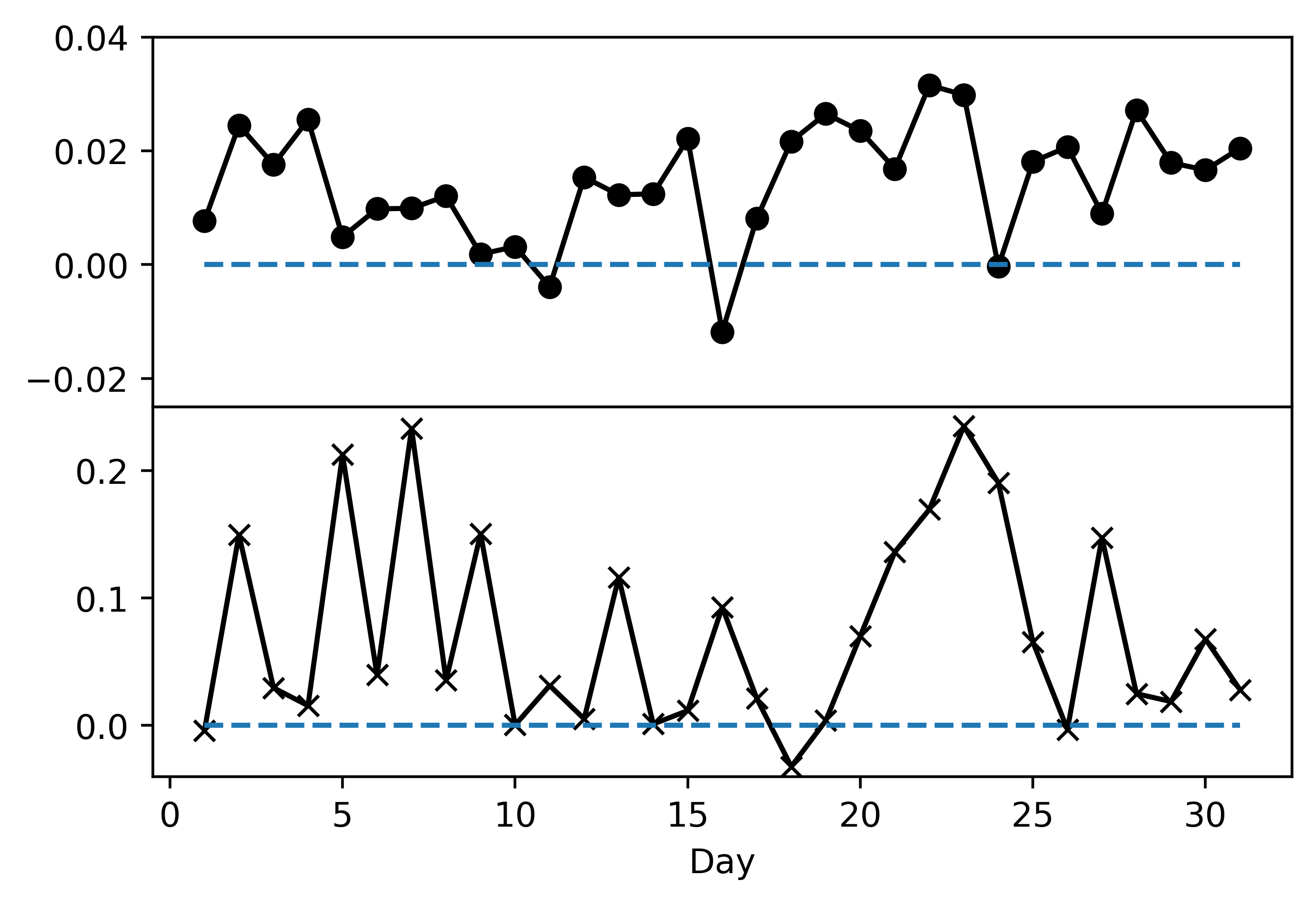
(a) Scenario 1

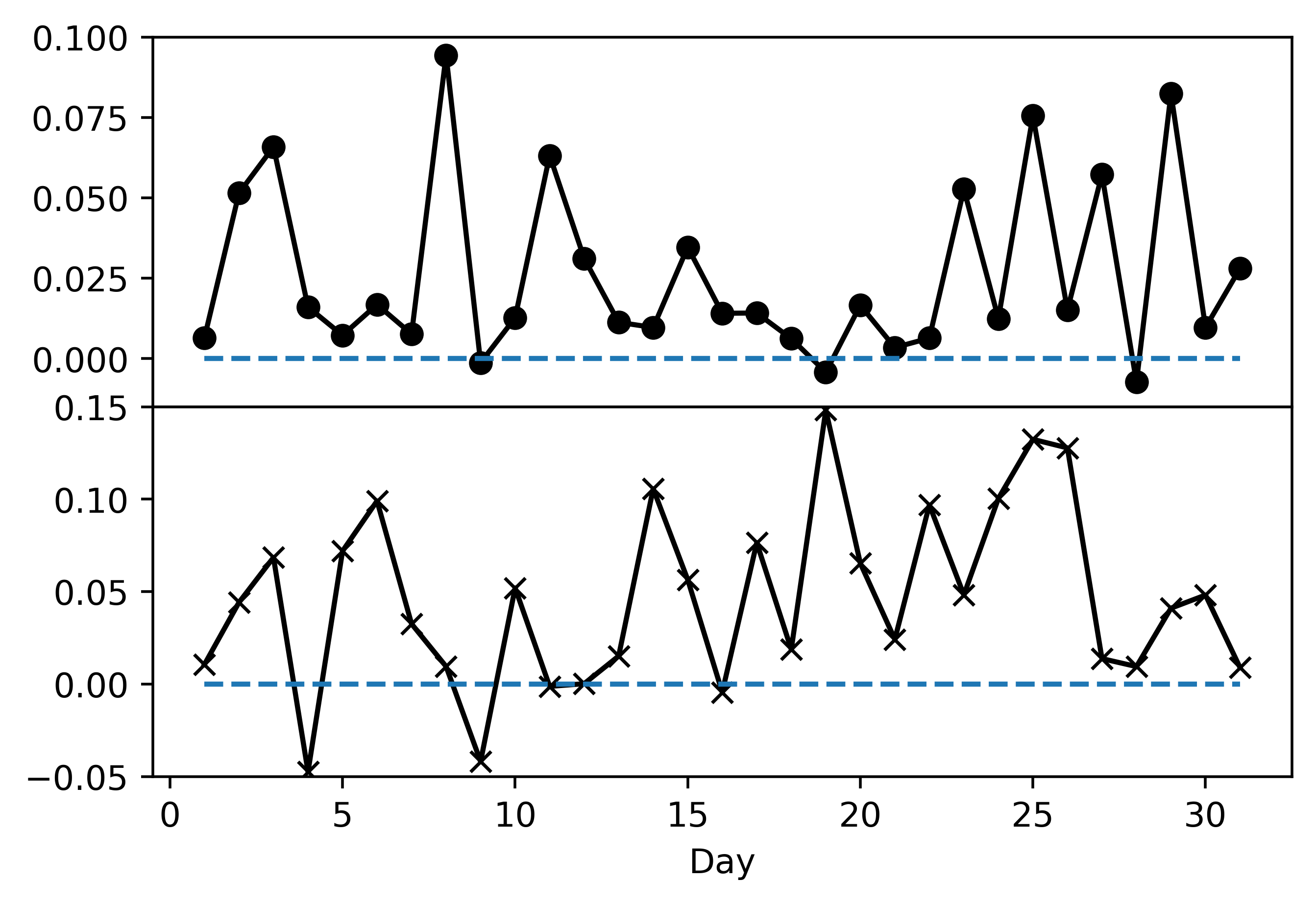
(b) Scenario 2

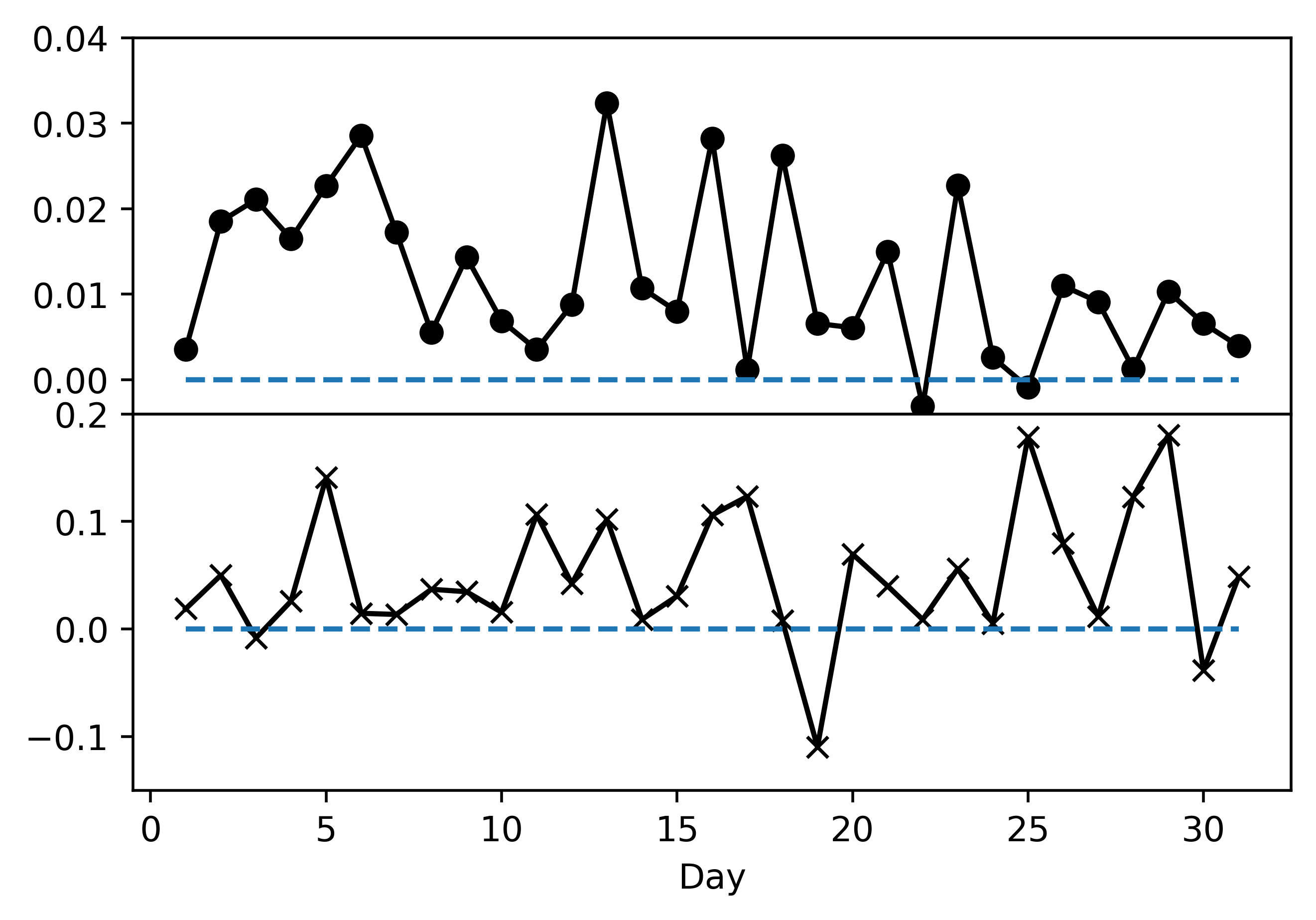
(c) Scenario 3

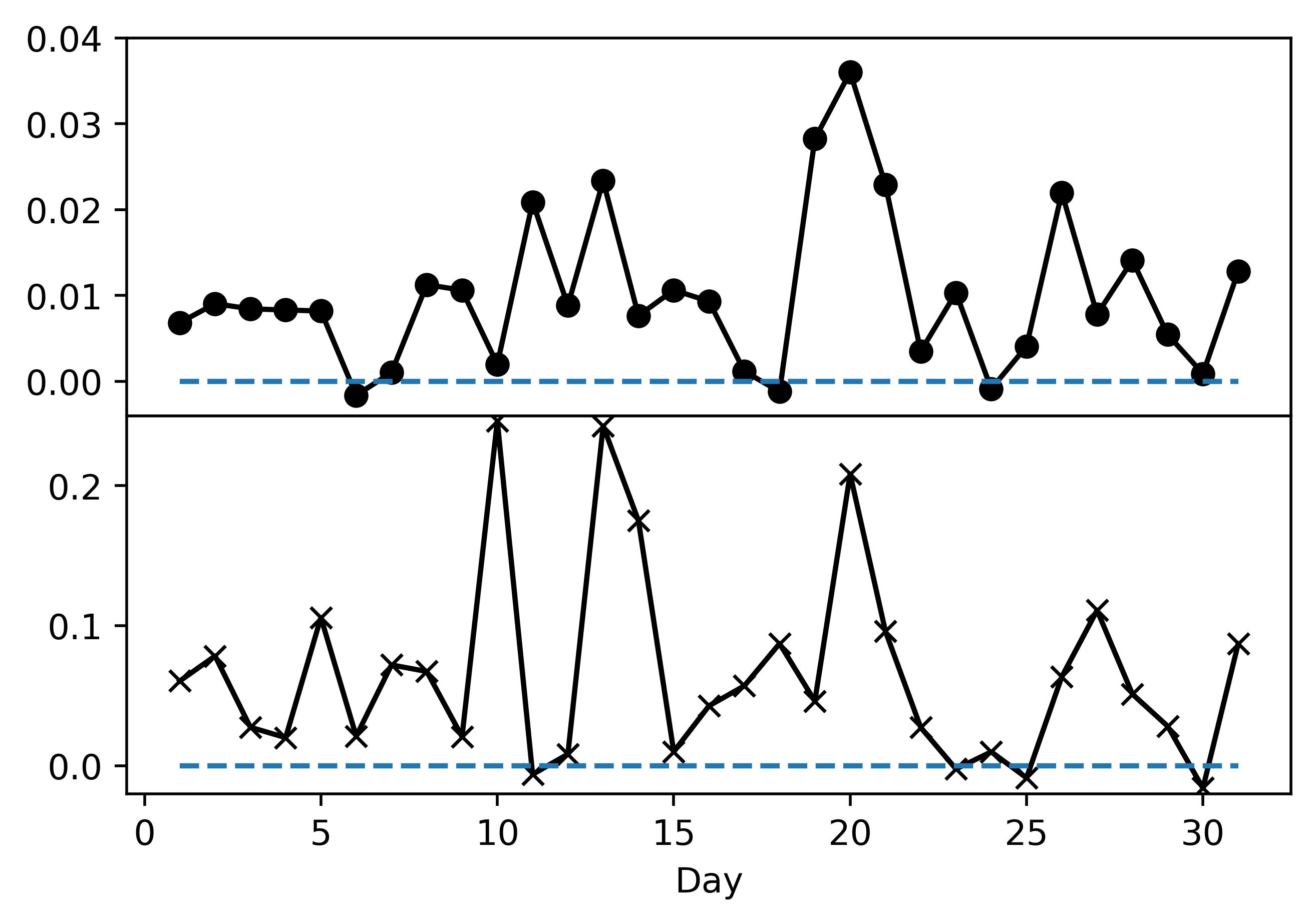
(d) Scenario 4

Figure 7: Online relative improvement ratios in four scenarios in consecutive four weeks. (Upper is the CTR improvement, Bottom is the PAPM improvement).

6 Conclusion

In this paper, we propose a framework named OptMSM, which can optimize multi-scenario modeling with disentangled representation and scenario-specific interaction. First, we partition input features into two separate feature sets incorporating scenario priors, including scenario-specific and scenario-shared features. Then we design a scenario-enhanced learning module with plugged scenario-shared information transfer. With orthogonal constraints on both scenario-aware representation and contrastive representations, we obtain the disentangled representation. Finally, the scenario-specific interaction module adopts hypernetwork to make the scenario-specific information and scenario-aware representation fully interact. Compelling results from both offline evaluation and online A/B experiments validate the effectiveness of our framework.

References

- [1] Abadi, M., Barham, P., Chen, J., Chen, Z., Davis, A., Dean, J., Devin, M., Ghemawat, S., Irving, G., Isard, M., Kudlur, M., Levenberg, J., Monga, R., Moore, S., Murray, D.G., Steiner, B., Tucker, P., Vasudevan, V., Warden, P., Wicke, M., Yu, Y., Zheng, X.: Tensorflow: A system for large-scale machine learning. In: Proceedings of the 12th USENIX Conference on Operating Systems Design and Implementation. p. 265–283. OSDI’16, USENIX Association, USA (2016)
- [2] Chang, J., Zhang, C., Hui, Y., Leng, D., Niu, Y., Song, Y.: Pepnet: Parameter and embedding personalized network for infusing with personalized prior information. arXiv preprint arXiv:2302.01115 (2023)
- [3] Chapelle, O., Manavoglu, E., Rosales, R.: Simple and scalable response prediction for display advertising. ACM Trans. Intell. Syst. Technol. 5(4), 61 (dec 2015)
- [4] Chen, W., Hsu, W., Lee, M.: Making recommendations from multiple domains. In: The 19th ACM SIGKDD International Conference on Knowledge Discovery and Data Mining, KDD 2013. pp. 892–900. ACM, Chicago, IL, USA (2013). https://doi.org/10.1145/2487575.2487638
- [5] Cheng, H., Koc, L., Harmsen, J., Shaked, T., Chandra, T., Aradhye, H., Anderson, G., Corrado, G., Chai, W., Ispir, M., Anil, R., Haque, Z., Hong, L., Jain, V., Liu, X., Shah, H.: Wide & deep learning for recommender systems. In: Proceedings of the 1st Workshop on Deep Learning for Recommender Systems, DLRS@RecSys 2016. pp. 7–10. ACM, Boston, MA, USA (2016)
- [6] Feng, J., Li, H., Huang, M., Liu, S., Ou, W., Wang, Z., Zhu, X.: Learning to collaborate: Multi-scenario ranking via multi-agent reinforcement learning. In: Proceedings of the 2018 World Wide Web Conference. p. 1939–1948. WWW ’18, International World Wide Web Conferences Steering Committee, Republic and Canton of Geneva, CHE (2018). https://doi.org/10.1145/3178876.3186165
- [7] Gu, Y., Bao, W., Ou, D., Li, X., Cui, B., Ma, B., Huang, H., Liu, Q., Zeng, X.: Self-supervised learning on users’ spontaneous behaviors for multi-scenario ranking in e-commerce. In: Proceedings of the 30th ACM International Conference on Information & Knowledge Management. p. 3828–3837. CIKM ’21, Association for Computing Machinery, New York, NY, USA (2021). https://doi.org/10.1145/3459637.3481953
- [8] Guo, H., Tang, R., Ye, Y., Li, Z., He, X.: Deepfm: A factorization-machine based neural network for CTR prediction. In: 26th International Joint Conference on Artificial Intelligence, IJCAI 2017. pp. 1725–1731. ijcai.org, Melbourne, Australia (2017)
- [9] Ha, D., Dai, A.M., Le, Q.V.: Hypernetworks. In: International Conference on Learning Representations (2017)
- [10] Hu, J., Shen, L., Sun, G.: Squeeze-and-excitation networks. In: Proceedings of the IEEE Conference on Computer Vision and Pattern Recognition (CVPR) (June 2018)
- [11] Jiang, Y., Li, Q., Zhu, H., Yu, J., Li, J., Xu, Z., Dong, H., Zheng, B.: Adaptive domain interest network for multi-domain recommendation. In: Proceedings of the 31st ACM International Conference on Information & Knowledge Management. p. 3212–3221. CIKM ’22, Association for Computing Machinery, New York, NY, USA (2022). https://doi.org/10.1145/3511808.3557137
- [12] Kingma, D.P., Ba, J.: Adam: A method for stochastic optimization. In: Bengio, Y., LeCun, Y. (eds.) 3rd International Conference on Learning Representations, ICLR 2015, San Diego, CA, USA, May 7-9, 2015, Conference Track Proceedings (2015)
- [13] Li, P., Li, R., Da, Q., Zeng, A., Zhang, L.: Improving multi-scenario learning to rank in e-commerce by exploiting task relationships in the label space. In: CIKM ’20: The 29th ACM International Conference on Information and Knowledge Management. pp. 2605–2612. ACM, Virtual Event, Ireland (2020). https://doi.org/10.1145/3340531.3412713
- [14] Liu, B., Zhu, C., Li, G., Zhang, W., Lai, J., Tang, R., He, X., Li, Z., Yu, Y.: Autofis: Automatic feature interaction selection in factorization models for click-through rate prediction. In: KDD ’20: The 26th ACM SIGKDD Conference on Knowledge Discovery and Data Mining. pp. 2636–2645. ACM, USA (2020)
- [15] Lyu, F., Tang, X., Guo, H., Tang, R., He, X., Zhang, R., Liu, X.: Memorize, factorize, or be naive: Learning optimal feature interaction methods for CTR prediction. In: 38th IEEE International Conference on Data Engineering, ICDE 2022. pp. 1450–1462. IEEE, Kuala Lumpur, Malaysia (2022). https://doi.org/10.1109/ICDE53745.2022.00113
- [16] Lyu, F., Tang, X., Liu, D., Wu, H., Ma, C., He, X., Liu, X.: Feature representation learning for click-through rate prediction: A review and new perspectives. CoRR abs/2302.02241 (2023). https://doi.org/10.48550/arXiv.2302.02241, https://doi.org/10.48550/arXiv.2302.02241
- [17] Ma, J., Zhao, Z., Yi, X., Chen, J., Hong, L., Chi, E.H.: Modeling task relationships in multi-task learning with multi-gate mixture-of-experts. In: Proceedings of the 24th ACM SIGKDD International Conference on Knowledge Discovery & Data Mining. p. 1930–1939. KDD ’18, Association for Computing Machinery, New York, NY, USA (2018). https://doi.org/10.1145/3219819.3220007
- [18] Van der Maaten, L., Hinton, G.: Visualizing data using t-sne. Journal of machine learning research 9(11) (2008)
- [19] Naumov, M., Mudigere, D., Shi, H.M., Huang, J., Sundaraman, N., Park, J., Wang, X., Gupta, U., Wu, C., Azzolini, A.G., Dzhulgakov, D., Mallevich, A., Cherniavskii, I., Lu, Y., Krishnamoorthi, R., Yu, A., Kondratenko, V., Pereira, S., Chen, X., Chen, W., Rao, V., Jia, B., Xiong, L., Smelyanskiy, M.: Deep learning recommendation model for personalization and recommendation systems. CoRR abs/1906.00091 (2019)
- [20] Niu, X., Li, B., Li, C., Tan, J., Xiao, R., Deng, H.: Heterogeneous graph augmented multi-scenario sharing recommendation with tree-guided expert networks. In: Proceedings of the 14th ACM International Conference on Web Search and Data Mining. p. 1038–1046. WSDM ’21, Association for Computing Machinery, New York, NY, USA (2021). https://doi.org/10.1145/3437963.3441729
- [21] Ranasinghe, K., Naseer, M., Hayat, M., Khan, S., Khan, F.S.: Orthogonal projection loss. In: Proceedings of the IEEE/CVF International Conference on Computer Vision (ICCV). pp. 12333–12343 (October 2021)
- [22] Rendle, S.: Factorization machines. In: ICDM 2010, The 10th IEEE International Conference on Data Mining. pp. 995–1000. IEEE Computer Society, Sydney, Australia (2010)
- [23] Richardson, M., Dominowska, E., Ragno, R.: Predicting clicks: estimating the click-through rate for new ads. In: Proceedings of the 16th International Conference on World Wide Web, WWW 2007. pp. 521–530. ACM, Banff, Alberta, Canada (2007). https://doi.org/10.1145/1242572.1242643
- [24] Shen, Q., Tao, W., Zhang, J., Wen, H., Chen, Z., Lu, Q.: Sar-net: A scenario-aware ranking network for personalized fair recommendation in hundreds of travel scenarios. In: Proceedings of the 30th ACM International Conference on Information & Knowledge Management. p. 4094–4103. CIKM ’21, Association for Computing Machinery, New York, NY, USA (2021). https://doi.org/10.1145/3459637.3481948
- [25] Sheng, X., Zhao, L., Zhou, G., Ding, X., Dai, B., Luo, Q., Yang, S., Lv, J., Zhang, C., Deng, H., Zhu, X.: One model to serve all: Star topology adaptive recommender for multi-domain CTR prediction. In: CIKM ’21: The 30th ACM International Conference on Information and Knowledge Management. pp. 4104–4113. ACM, Virtual Event, Queensland, Australia (2021). https://doi.org/10.1145/3459637.3481941
- [26] Tang, H., Liu, J., Zhao, M., Gong, X.: Progressive layered extraction (ple): A novel multi-task learning (mtl) model for personalized recommendations. In: Proceedings of the 14th ACM Conference on Recommender Systems. p. 269–278. RecSys ’20, Association for Computing Machinery, New York, NY, USA (2020). https://doi.org/10.1145/3383313.3412236
- [27] Vaswani, A., Shazeer, N., Parmar, N., Uszkoreit, J., Jones, L., Gomez, A.N., Kaiser, L.u., Polosukhin, I.: Attention is all you need. In: Guyon, I., Luxburg, U.V., Bengio, S., Wallach, H., Fergus, R., Vishwanathan, S., Garnett, R. (eds.) Advances in Neural Information Processing Systems. vol. 30. Curran Associates, Inc. (2017)
- [28] Wang, F., Wang, Y., Li, D., Gu, H., Lu, T., Zhang, P., Gu, N.: Cl4ctr: A contrastive learning framework for ctr prediction. In: Proceedings of the Sixteenth ACM International Conference on Web Search and Data Mining. p. 805–813. WSDM ’23, Association for Computing Machinery, New York, NY, USA (2023). https://doi.org/10.1145/3539597.3570372
- [29] Wang, R., Fu, B., Fu, G., Wang, M.: Deep & cross network for ad click predictions. In: Proceedings of the ADKDD’17. ADKDD’17, Association for Computing Machinery, Canada (2017)
- [30] Wang, R., Shivanna, R., Cheng, D., Jain, S., Lin, D., Hong, L., Chi, E.: Dcn v2: Improved deep & cross network and practical lessons for web-scale learning to rank systems. In: Proceedings of the Web Conference 2021. p. 1785–1797. WWW ’21, Association for Computing Machinery, New York, NY, USA (2021). https://doi.org/10.1145/3442381.3450078
- [31] Wang, Y., Guo, H., Chen, B., Liu, W., Liu, Z., Zhang, Q., He, Z., Zheng, H., Yao, W., Zhang, M., Dong, Z., Tang, R.: Causalint: Causal inspired intervention for multi-scenario recommendation. In: Proceedings of the 28th ACM SIGKDD Conference on Knowledge Discovery and Data Mining. p. 4090–4099. KDD ’22, Association for Computing Machinery, New York, NY, USA (2022). https://doi.org/10.1145/3534678.3539221
- [32] Xi, D., Chen, Z., Yan, P., Zhang, Y., Zhu, Y., Zhuang, F., Chen, Y.: Modeling the sequential dependence among audience multi-step conversions with multi-task learning in targeted display advertising. In: Proceedings of the 27th ACM SIGKDD Conference on Knowledge Discovery & Data Mining. p. 3745–3755. KDD ’21, Association for Computing Machinery, New York, NY, USA (2021). https://doi.org/10.1145/3447548.3467071
- [33] Yan, B., Wang, P., Zhang, K., Li, F., Deng, H., Xu, J., Zheng, B.: APG: Adaptive parameter generation network for click-through rate prediction. In: Oh, A.H., Agarwal, A., Belgrave, D., Cho, K. (eds.) Advances in Neural Information Processing Systems (2022)
- [34] Zhang, Q., Liao, X., Liu, Q., Xu, J., Zheng, B.: Leaving no one behind: A multi-scenario multi-task meta learning approach for advertiser modeling. In: Proceedings of the Fifteenth ACM International Conference on Web Search and Data Mining. p. 1368–1376. WSDM ’22, Association for Computing Machinery, New York, NY, USA (2022). https://doi.org/10.1145/3488560.3498479
- [35] Zhang, W., Qin, J., Guo, W., Tang, R., He, X.: Deep learning for click-through rate estimation. In: Proceedings of the Thirtieth International Joint Conference on Artificial Intelligence, IJCAI-21. pp. 4695–4703. International Joint Conferences on Artificial Intelligence Organization, Montreal, Quebec, Canada (8 2021). https://doi.org/10.24963/ijcai.2021/636, survey Track
- [36] Zhang, Y., Yang, Q.: A survey on multi-task learning. IEEE Transactions on Knowledge and Data Engineering 34(12), 5586–5609 (2022). https://doi.org/10.1109/TKDE.2021.3070203
- [37] Zhang, Y., Wang, X., Hu, J., Gao, K., Lei, C., Fang, F.: Scenario-adaptive and self-supervised model for multi-scenario personalized recommendation. In: Proceedings of the 31st ACM International Conference on Information & Knowledge Management. p. 3674–3683. CIKM ’22, Association for Computing Machinery, New York, NY, USA (2022). https://doi.org/10.1145/3511808.3557154
- [38] Zou, X., Hu, Z., Zhao, Y., Ding, X., Liu, Z., Li, C., Sun, A.: Automatic expert selection for multi-scenario and multi-task search. In: Proceedings of the 45th International ACM SIGIR Conference on Research and Development in Information Retrieval. p. 1535–1544. SIGIR ’22, Association for Computing Machinery, New York, NY, USA (2022). https://doi.org/10.1145/3477495.3531942