Generative modeling of nucleon-nucleon interactions

Abstract

Developing high-precision models of the nuclear force and propagating the associated uncertainties in quantum many-body calculations of nuclei and nuclear matter remain key challenges for ab initio nuclear theory. In the present work we demonstrate that generative machine learning models can construct novel instances of the nucleon-nucleon interaction when trained on existing potentials from the literature. In particular, we train the generative model on nucleon-nucleon potentials derived at second and third order in chiral effective field theory and at three different choices of the resolution scale. We then show that the model can be used to generate samples of the nucleon-nucleon potential drawn from a continuous distribution in the resolution scale parameter space. The generated potentials are shown to produce high-quality nucleon-nucleon scattering phase shifts. This work provides an important step toward a comprehensive estimation of theoretical uncertainties in nuclear many-body calculations that arise from the arbitrary choice of nuclear interaction and resolution scale.

Introduction: High-precision models of the nuclear interaction are essential not only for explaining the structure and dynamics of atomic nuclei but also for describing the properties of hot and dense matter in extreme astrophysical environments, such as neutron stars, core-collapse supernovae, and neutron star mergers. Since the nuclear potential arises from quantum chromodynamics (QCD) as the low-energy effective interaction among composite nucleons, there is an inherent uncertainty due to the choice of resolution scale at which nuclear dynamics is resolved. This resolution scale is typically parameterized in the nuclear potential through a momentum-space regulating function parameter $\Lambda$ that demarcates the separation between low-energy and high-energy (unresolved) physics. In practice, the results of nuclear many-body calculations are not invariant under this choice of scale. In recent years, chiral effective field theory (EFT) Weinberg (1979); Epelbaum et al. (2009); Machleidt and Entem has emerged as a suitable tool to systematically study not only the scale dependence of nuclear interactions but also to estimate uncertainties due to missing physics through an analysis of effective field theory truncation errors Epelbaum et al. (2015); Furnstahl et al. (2015a, b); Wesolowski et al. (2016); Carlsson et al. ; Drischler et al. (2019); Wesolowski et al. (2019); Drischler et al. (2020a, b, 2021, c); Melendez et al. (2017). In the framework of chiral EFT, a specific nuclear interaction is obtained by first defining the high-momentum regulating function and then fitting to two-body scattering and bound state data the low-energy constants (LECs) of the theory that characterize unresolved short-distance physics Entem and Machleidt ; Entem et al. ; Entem et al. (2015); Carlsson et al. .

Nuclear potentials from chiral EFT are typically fitted at only a few select values of $\Lambda$, from which one can obtain a qualitative estimate of the resolution scale uncertainties. For statistical inference, however, one requires the ability to draw samples of the nucleon-nucleon (NN) potential from a continuous distribution in $\Lambda$, denoted as $p(V_{\rm ChEFT}|\Lambda)$. In the present work, we show that modern machine learning generative models have the ability to learn salient features of the NN interaction, build distributions of potentials, and create novel and physically reasonable instances of the nuclear potential over a continuous range of resolution scales $\Lambda$. Generative models have become a popular research topic in machine learning due to their ability to generate new data based on existing data distributions, which has many practical applications to image and speech synthesis. In the field of computer vision, the Generative Flow (Glow) model Kingma and Dhariwal ; Dinh et al. (2017) has been shown to be a successful model for generating realistic images and manipulating their attributes. In the present work, we adapt and refine the Glow model to develop a generative machine learning model for nuclear potentials. Effectively, we will treat the momentum-space matrix elements of the potential in different partial waves as “images”. We show that the model can recreate the training potentials and generate new physically reasonable nucleon-nucleon potentials over a continuum of cutoff scales. The reliability of the generated potentials is benchmarked by calculating nucleon-nucleon scattering phase shifts. Finally, we show that a combination of the Glow model and Vision Transformer model Dosovitskiy et al. (2021) allows for the extraction of chiral EFT LECs from the generated nuclear potential matrix elements.

Methods: The Glow model attempts to learn the properties of a given dataset by constructing an appropriate probability distribution to estimate the probabilities of some features of a sample. Once an appropriate probability distribution is found, the Glow model can generate novel samples by drawing from the distribution through sampling. To achieve this goal, the Glow model initializes a trainable distribution whose parameters $\bm{\theta}$ are iteratively adjusted such that the likelihood of the distribution can be maximized with respect to $\bm{\theta}$. In terms of the log-likelihood, one minimizes Winkler et al. (2019)

$$\mathcal{L}(\bm{\theta}) =-\frac{1}{N}\sum_{i}\log p_{\bm{\theta}}(\bm{x}_{i})$$ (1)

where $p_{\bm{\theta}}(\bm{x}_{i})$ is the probability of the sample $\bm{x}_{i}$, and $\bm{\theta}$ represents trainable parameters.

As a flow-based model, Glow couples several layers of transformation functions to form the flow $f$. The flow transforms a sample $\bm{x}$ from the data space to the latent space variable $\bm{z}$ via

$$\bm{z} =f_{K}\circ f_{K-1}\circ\dots\circ f_{k}\circ\dots\circ f_{1}(\bm{x}),$$ (2)

where $f_{k}$ is the transformation function at the $k$-th layer. If the probability density function (PDF) of the latent space is given by $q_{\bm{\theta}}(\bm{z})$, then the probability of the sample can be calculated through

$$\log p_{\bm{\theta}}(\bm{x}) =\log q_{\bm{\theta}}(\bm{z})+\log|\det\differential\bm{z}/\differential\bm{x}|$$

$$=\log q_{\bm{\theta}}(\bm{z})+\sum_{k=1}^{K}\log|\det\differential\bm{h}_{k}/\differential\bm{h}_{k-1}|,$$ (3)

where $\bm{h}_{k}$ are the transformed variables at the $k$-th transformation layer, and $\bm{h}_{0}=\bm{x}$, $\bm{h}_{K}=\bm{z}$ for consistency. The distribution of the latent space should be tractable so that the Glow model can easily draw $\bm{z}$ from it. In addition, the transformation functions should be invertible so that the generated $\bm{z}$ can be transformed to the data space as $\bm{x}=f^{-1}(\bm{z})$.

In this work, a layer of transformation is composed of three parts: an ActNorm, a $1\times 1$ convolution transformation (1x1conv) Dinh et al. (2015), and a rational quadratic spline (RQS) transformation Gao et al. (2020); Durkan et al. (2019). At a transformation layer $f_{k}$, a variable gets transformed through a sequence of transformation as $\bm{h}_{k}=f_{k}(\bm{h}_{k-1})={\rm RQS}\circ{\rm 1x1conv}\circ{\rm ActNorm}(\bm{h}_{k-1})$. Since each of these three transformation functions are built based on trainable parameters and neural networks, the transformation layer can be trained to maximize the likelihood contributed from the second term in Eq. (Generative modeling of nucleon-nucleon interactions).

The Glow model incorporates multiple-scale architecture Dinh et al. (2017) for efficiency purposes. A sequence of operations is performed on each sample for every scale. The first operation, squeezing, changes the shape of a sample from $(C,H,W)$ to $(4\times C,H/2,W/2)$, where $C$ is the number of channels, and $H$ and $W$ are the height and weight, respectively. At the second operation, $K$ layers of transformation functions are coupled. The sample now is transformed according to Eq. (2). Upon reaching the end of the scale, the sample is again split into two halves along the channel dimension. The first half is treated as part of the fully transformed sample $\bm{z}$ in the resulting latent space. Its probability will be calculated by a tractable base distribution model whose parameters are the output of neural networks, and contribute to the total probability $q_{\theta}(\bm{z})$. The remaining half is employed as the input of the neural networks responsible for constructing the base distribution and will continue progressing to the next scale. A tensor with the shape of $(C,H,W)$ traverses through $L$-layer scales and finally there are still $(2^{L}\times C,H/2^{L},W/2^{L})$ elements whose distribution has not been determined. The base distribution to evaluate the probabilities of final elements is built by neural networks whose inputs are the labels of the sample. In our work, the base distributions are Gaussian distributions.

To produce samples with new labels, the key idea is to obtain samples in latent space and transform them back into data space. We can consider two different approaches: 1. latent space sampling (LSS) and 2. latent space interpolation (LSI). For the LSS, we follow a three-step process. First, we draw samples $\bm{z}$ in the latent space from a Gaussian which is built according to the labels from the training set. Next, we perform interpolation based on the obtained $\bm{z}$ samples and the new label. Finally, we transform the interpolated sample back into the data space, yielding the generated sample with the new label. Alternatively, for the LSI, the samples of $\bm{z}$ are obtained by transforming given $\bm{x}$s from the data space to the latent space. The next two steps are the same as in LSS approach. Note the first approach is suitable for drawing samples from distributions with desired labels, while the second approach can be applied to predict instances of samples based on existing samples. If the input samples in LSI are physically reasonable (for example, best-fitted chiral potentials at given $\Lambda$s), we expect the generated new samples should also be physically reasonable. Due to the dimension being reduced by a factor of $2^{L}$ from the data space to the latent space, the interpolation process becomes significantly simpler in the latent space. These two approaches provide methods to generate high-dimensional samples from complicated distributions. For nuclear interaction modeling, we view the partial wave matrix elements as the samples for the Glow model. Therefore, a nuclear potential can be viewed as a sample with shape $(C,H,W)$, where $C$ is the number of partial wave channels $\alpha$, and $H$ and $W$ are the number of momentum-space mesh points of $p$ and $p^{\prime}$ for the potential $V_{\alpha}(p,p^{\prime})$.

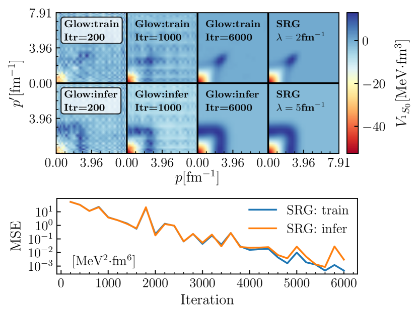
Figure 1: (Top) ${}^{1}S_{0}$ matrix elements of glow-generated SRG potentials at $\lambda=2$ and $5$ fm^-1 at different training iterations. The true SRG potential matrix elements are shown on the right side for comparison. (Bottom) The mean squared error, calculated based on the difference of all the elements from all the corresponding potentials.

Results: We conduct two experiments to investigate the Glow model’s capabilities in reconstructing actual nuclear potentials, building distributions, and generating new, realistic ones. Our first experiment is based on potentials generated from the Similarity Renormalization Group (SRG) Bogner et al. (2007); Jurgenson et al. , where the resolution scale can be freely chosen. In the SRG, a potential $V_{\lambda}$ is evolved with a flow parameter $\lambda$ from an initial potential $V$ by a unitary transformation. The transformation is designed to reduce the high-momentum off-diagonal parts of $V_{\lambda}$ as $\lambda$ decreases. In this paper, the initial potential for the SRG is the next-to-next-to-next-to-leading order (n3lo) chiral nuclear potential of Entem and Machleidt Entem and Machleidt (2003) with momentum-space cutoff $\Lambda=500$ MeV, which we denote in this work by “EM500”. The second experiment attempts to train the Glow model to learn the characteristics of chiral potentials n$\nu$lo$\Lambda$ at different orders $\nu$ in the chiral expansion and different high-momentum cutoff values $\Lambda$.

To train a Glow model for the SRG, we gather potentials with $\lambda\in\{2,3,4,7,8,10,11,12\}\,{\rm fm}^{-1}$. We then employ the Glow model to deduce potentials with $\lambda={5,6,9,13}\,{\rm fm}^{-1}$ using LSI throughout the training to evaluate the model’s inference capability. When using LSI, the input potentials are the actual SRG potentials used for training. We calculate the mean square error (MSE) by measuring the difference between all the matrix elements of Glow-generated potentials and the actual potentials from SRG. In the bottom subfigure of Fig. 1, we show the MSE as a function of training iteration. During the training process, both the reconstructed potentials (blue line) and the inferred potentials (orange line) converge toward the true potentials generated by the SRG, as indicated by the decreasing MSE. The top subfigure of Fig. 1 shows the Glow-generated SRG potential matrix elements in the ${}^{1}S_{0}$ partial wave at different iterations (3 columns on the left) and the actual potentials from SRG (rightmost column). Initially, the Glow model only generates Gaussian noise. Upon completion of the training, the potentials obtained from the Glow model and the SRG appear indistinguishable.

Next, we train a separate Glow model based on a set of six chiral potentials with truncation orders $\nu\in\{2,3\}$ and cutoffs $\Lambda\in\{450,500,550\}\,{\rm MeV}$ Entem et al. (2017). In this scenario, the samples for each set of labels $({\nu,\lambda})$ are generated using normally distributed LECs, which mimic the uncertainties from fitting to phase shifts and bound state data Wesolowski et al. (2019). The mean values of these LECs correspond to the actual chiral potentials at every set of $(\nu,\Lambda)$. Since the chiral potentials generated by the Glow model are just given in terms of their partial-wave matrix elements, we have also trained a Vision Transformer (ViT) model Dosovitskiy et al. (2021); Vaswani et al. (2017) to deduce the associated LECs and value of $\Lambda$ from Glow-generated potentials. The ViT model is a widely used machine learning model that is well-suited for regression and classification tasks. In the present case, the ViT model is trained on a large dataset of (unphysical) chiral potentials with LECs randomly sampled from a uniform distribution. The training process continues until we find that the ViT model is able to extract the LECs and $\Lambda$ values precisely.

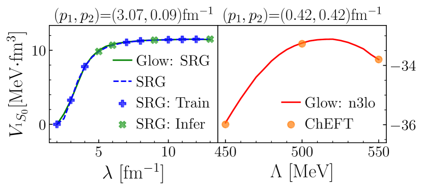
Figure 2: SRG (left) and chiral (right) potential matrix elements in the ${}^{1}S_{0}$ partial-wave channel. Plus, dot, cross markers and dashed lines are from actual potentials, while solid lines are generated by trained Glow models using LSI.

In Fig. 2, we show the cutoff dependence of selected ${}^{1}S_{0}$ partial-wave matrix elements of the Glow-generated SRG potentials (left panel) and chiral potentials (right panel) using LSI, where the inputs for LSI are the actual pre-existing potentials. In the left panel, the plus and cross symbols mark the actual values of the SRG potential matrix elements at the values of $\lambda$ used for training (plus) and validation (cross), which naturally lie exactly on the dashed-blue line that indicates the actual SRG matrix elements as a function of $\lambda$. The matrix elements from the Glow model are shown with the solid green line, which lies nearly on top of the blue dashed line of the actual SRG matrix elements. We note that the Glow model is not simply interpolating between training points, since the two validation points at $\lambda=5,6$ fm^-1 would then be much farther from the blue-dashed SRG line. In addition, the far off-diagonal matrix element $\langle p^{\prime}=3.07\,\text{fm}^{-1}|V_{{}^{1}S_{0}}|p=0.09\,\text{fm}^{-1}\rangle$ of the SRG potentials should decay strongly with decreasing $\lambda$ as $V_{\lambda}(p_{1},p_{2})\approx V(p_{1},p_{2})e^{-(p_{1}^{2}-p_{2}^{2})^{2}/\lambda^{4}}$ Bogner et al. . From the left panel of Fig. 2 we see that this particular feature of SRG potentials is accurately reproduced by the Glow model. Similarly, in the right panel of Fig. 2, we see that the chiral EFT diagonal matrix elements $\langle p^{\prime}=0.422\,\text{fm}^{-1}|V_{{}^{1}S_{0}}|p=0.422\,\text{fm}^{-1}\rangle$ generated by the Glow model across a continuum of $\Lambda$ values follow a smooth contour that pass through the actual values at $\Lambda=450,500,550$ MeV.

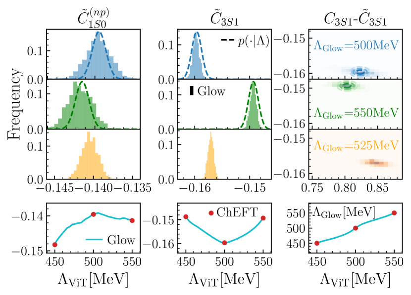
Figure 3: (Top three rows) LEC distributions predicted by LSS for n3lo chiral potentials with $\Lambda=500,550,525$ MeV. In the top two panels we show for comparison the input distributions as dashed lines. (Bottom) Peak LEC values and cutoffs of potentials generated from LSI, where the inputs for LSI are actual chiral potentials. All the LECs and cutoffs are extracted by a trained ViT model from Glow-generated potentials. The red dots are the LECs and cutoffs for the actual chiral n3lo potentials.

In Fig. 3 we show the conditional distributions of LECs for given $\Lambda$s in the first three rows. The potentials are sampled using the LSS method and the LECs are extracted by the trained ViT model. We find that the Glow model has the ability to rebuild the LEC distribution at the training values of $\Lambda=500,550$  MeV (top two rows) since the frequencies of LECs follows closely the actual distribution of LECs (dashed curves). We also show in the third row the predicted distribution $p({\rm LECs}|\Lambda=525{\rm MeV})$. The central point of the predicted distribution is positioned within the range between the centers of $p({\rm LECs}|\Lambda=500{\rm MeV})$ and $p({\rm LECs}|\Lambda=550{\rm MeV})$. Moreover, the width of uncertainty in the predicted distribution is comparable to the width of uncertainty observed in the distributions used to train the Glow model. These facts suggest that the predicted distribution is reasonable and aligned with the expected behavior of the dataset. Finally, the fourth row shows the continuous evolution of the peak in the LEC distributions between $\Lambda=450-550$ MeV, where the actual values are shown as red dots for comparison. We find that the Glow model can accurately regenerate the known chiral potentials at $\Lambda=450,500,550$ MeV and the ViT can recover the known LECs. We also show in the bottom-right panel of Fig. 3 the relation between the cutoff $\Lambda_{\rm Glow}$ as the input label for the Glow model and the cutoff $\Lambda_{\rm ViT}$ predicted by the ViT model. The near identity between the two $\Lambda$ values shows that the Glow model can generate chiral potentials with the desired value of $\Lambda$ and that the ViT model can accurately extract $\Lambda$ from the potential matrix elements.

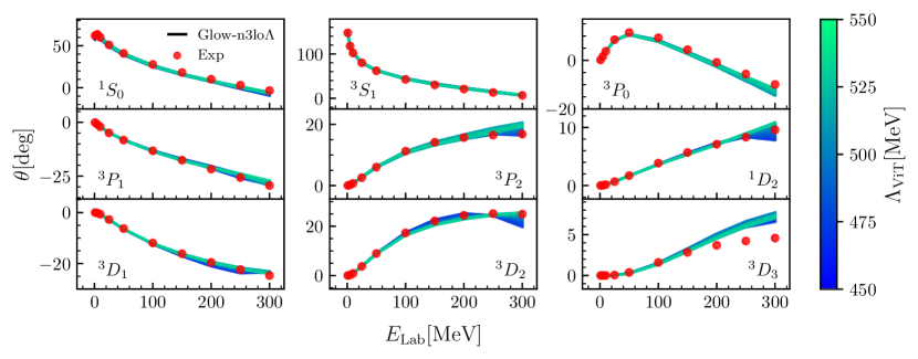
Figure 4: Phase shifts for $np$ scattering. The colored solid lines correspond to Glow-n3lo$\Lambda$ potentials. Red dots correspond to the phase shift analysis Navarro Pérez et al. (2014) of NN scattering data.

To verify the quality of the chiral potentials generated by the Glow model, in Fig. 4 we show the calculated phase shifts in the lowest partial-wave channels. Rather than directly using the Glow-generated potential matrix elements in the calculation of the phase shifts, we instead construct a new chiral potential at n3lo from the low-energy constants and cutoff value $\Lambda$ inferred from the ViT model. We denote the new chiral potentials as “Glow-${\rm n}3{\rm lo}\Lambda$”. From Fig. 4 we observe that the Glow-${\rm n}3{\rm lo}\Lambda$ potentials give good phase shift results when compared to experimental data used to fit the actual chiral potentials. Furthermore, even though the values of $\Lambda$ are uniformly sampled over the range $450<\Lambda<550$, the phase shifts need not be uniformly distributed. As an illustration, in channel ${}^{1}D_{2}$ the density of lines cluster near the upper and lower limits. Thus, the Glow model may be used for an improved statistical treatment of uncertainties that arise due to the arbitrary choice of cutoff in chiral EFT interactions.

Summary and Outlook: In this work, we have extended the Glow generative model to the case of nucleon-nucleon interactions. The results demonstrate that the Glow model is not only capable of accurately reconstructing nuclear potentials, but also capable of generating new potentials or building the distribution of potentials at intermediate values of the momentum-space cutoff $\Lambda$. The ability to reconstruct and infer potentials is attained by learning the properties of nuclear potentials via maximum likelihood, where the probabilities are estimated by the trainable flows and base distributions. The Glow model trained on SRG potentials was shown to reproduce well the matrix elements at intermediate values of the flow parameter $\lambda$, including the suppression of potential matrix elements far off the diagonal. We have also trained the Glow model on chiral potentials at two different orders in the chiral expansion and three different choices of the momentum-space cutoff $\Lambda$. The ViT regression model enabled the construction of additional chiral potentials for Glow training and could be used to infer chiral EFT low-energy constants and cutoffs on Glow-generated potentials over a continuum of $\Lambda$ values. Finally, the Glow-n3lo$\Lambda$ potentials were shown to reproduce very well nucleon-nucleon scattering phase shifts.

The Glow model offers an efficient means for generating realistic chiral potentials in a matter of seconds. It therefore has the potential to serve as an effective tool to more reliably assess uncertainties due to the arbitrary choice of resolution scale in modern nucleon-nucleon potentials. In addition, we have shown that the Glow model can utilize information about LEC distributions at training values of $\Lambda$ to generate LEC distributions at new values of $\Lambda$. By coupling this approach with LEC parameter estimation obtained from fitting to NN data Carlsson et al. , a more comprehensive estimate of chiral effective field theory uncertainties can be achieved.