PyKoopman: A Python Package for Data-Driven Approximation of the Koopman Operator

Abstract

PyKoopman is a Python package for the data-driven approximation of the Koopman operator associated with a dynamical system. The Koopman operator is a principled linear embedding of nonlinear dynamics and facilitates the prediction, estimation, and control of strongly nonlinear dynamics using linear systems theory. In particular, PyKoopman provides tools for data-driven system identification for unforced and actuated systems that build on the equation-free dynamic mode decomposition (DMD) [1] and its variants [2, 3, 4]. In this work, we provide a brief description of the mathematical underpinnings of the Koopman operator, an overview and demonstration of the features implemented in PyKoopman (with code examples), practical advice for users, and a list of potential extensions to PyKoopman. Software is available at https://github.com/dynamicslab/pykoopman.

Keywords– system identification, dynamical systems, Koopman operator, open source, python

1 Introduction

Engineers have long relied on linearization to bridge the gap between simplified, linear descriptions where powerful analytical tools exist, and the intricate complexities of nonlinear dynamics where analytical solutions are elusive [5, 6]. Local linearization, implemented via first-order Taylor series approximation, has been widely used in system identification [5], optimization [6], and many other fields to make problems tractable. However, many real-world systems are fundamentally nonlinear and require solutions outside of the local neighborhood where linearization is valid. Rapid progress in machine learning and big data methods are driving advances in the data-driven modeling of such nonlinear systems in science and engineering [7] Koopman operator theory in particular has emerged as a principled approach to embed nonlinear dynamics in a linear framework that goes beyond simple linearization [4].

In the diverse landscape of data-driven modeling approaches, Koopman operator theory has received considerable attention in recent years [8, 9, 10, 11, 12, 13]. These strategies encompass not only linear methodologies [14, 5] and dynamic mode decomposition (DMD) [1, 15, 2], but also more advanced techniques such as nonlinear autoregressive algorithms [16, 17], neural networks [18, 19, 20, 21, 22, 23, 24, 25, 26, 27], Gaussian process regression [28], operator inference, and reduced-order modeling [29, 30, 31], among others [32, 33, 34, 35, 36, 37, 38]. The Koopman operator perspective is unique within data-driven modeling techniques due to its distinct aim of learning a coordinate system in which the nonlinear dynamics become linear. This methodology enables the application of closed-form, convergence-guaranteed methods from linear system theory to general nonlinear dynamics. To fully leverage the potential of data-driven Koopman theory across a diverse range of scientific and engineering disciplines, it is critical to have a central toolkit to automate state-of-the-art Koopman operator algorithms.

PyKoopman is a Python package designed to approximate the Koopman operator associated with both natural and actuated dynamical systems from measurement data. Specifically, PyKoopman offers tools for designing observables (i.e., functions of the system state) and inferring a finite-dimensional linear operator that governs the dynamic evolution of these observables in time. These steps can either be conducted sequentially [39, 10] or combined, as demonstrated in more recent neural network models [40, 41, 21, 42]. Once a linear embedding is discovered from the data, the linearity of the transformed dynamical system can be leveraged for enhanced interpretability [43] or for designing near-optimal observers [44] or controllers for the original nonlinear system [45, 46, 47, 48, 49].

The PyKoopman package is designed for both researchers and practitioners, enabling anyone with access to data to discover embeddings of nonlinear systems where the dynamics become approximately linear. Following PySINDy [50] and Deeptime [51], PyKoopman is structured to be user-friendly for those with basic knowledge of linear systems, adhering to scikit-learn standards, while also offering modular components for more advanced users.

2 Background

PyKoopman provides Python implementations of several leading algorithms for the data-driven approximation of the Koopman operator associated with a dynamical system

$$\frac{d}{dt}\mathbf{x}(t)=\mathbf{f}(\mathbf{x}(t),\mathbf{u}(t)),$$ (1)

where $\mathbf{x}\in\mathcal{M}\subseteq\mathbb{R}^{n}$ is the state of the system and $\mathbf{f}$ is a vector field describing the dynamics and the effect of control input $\mathbf{u}\in\mathbb{R}^{q}$. For the sake of simplicity, we will only present the background for the autonomous dynamical system, and more details for non-autonomous dynamical systems can be found in appendix A.

Consider the autonomous system

$$\frac{d}{dt}\mathbf{x}(t)=\mathbf{f}(\mathbf{x}(t)).$$ (2)

Data are typically sampled discretely in time in intervals of $\Delta t$, and the corresponding discrete-time dynamical system is given by the nonlinear map $\mathbf{F}:\mathcal{M}\mapsto\mathcal{M}$,

$$\mathbf{x}(t+\Delta t)=\mathbf{F}(\mathbf{x}(t)),$$ (3)

where $\mathbf{F}(\mathbf{x})=\mathbf{x}(t)+\int_{t}^{t+\Delta t}\mathbf{f}(\mathbf{x}(s))\,ds$.

Figure 1: Lifting of the state $\mathbf{x}$ of the continuous autonomous dynamical system in eq. 2 into a new coordinate system, in which the original nonlinear dynamics become linear and are easier to handle. One can also linearly reconstruct the state $\mathbf{x}$ from the new coordinate system. This is facilitated with PyKoopman in a data-driven manner.

Given data in the form of measurement vectors $\mathbf{x}(t)$, the goal of data-driven Koopman theory (see fig. 1) is to find a new coordinate system

$$\mathbf{z}:=\bm{\Phi}(\mathbf{x}),$$ (4)

where the dynamics are simplified, or ideally, linearized in the sense of either continuous dynamics,

$$\frac{d}{dt}\mathbf{z}=\mathbf{A}_{c}\mathbf{z},$$ (5)

or discrete-time dynamics,

$$\mathbf{z}(t+\Delta t)=\mathbf{A}\mathbf{z}(t),$$ (6)

where the subscript $c$ is for continuous-time and $\mathbf{A}=\exp({\Delta t\mathbf{A}_{c}})$. For simplicity, PyKoopman is focused on the discrete dynamical system in eq. 6, which is consistent with the majority of the literature [2, 3, 4].

The goal of learning the coordinates $\bm{\Phi}$ and linear dynamics $\mathbf{A}$ may be posed as a regression problem in terms of finding the linear operator that best maps the state of the system, or a transformed version of the state, forward in time. This may be formulated in terms of the following two data matrices,

$$\mathbf{X}=\begin{bmatrix}\vline&\vline&&\vline\\ \mathbf{x}(t_{1})&\mathbf{x}(t_{2})&\cdots&\mathbf{x}(t_{m})\\ \vline&\vline&&\vline\end{bmatrix},\quad\mathbf{X}^{\prime}=\begin{bmatrix}\vline&\vline&&\vline\\ \mathbf{x}(t_{1}^{\prime})&\mathbf{x}(t_{2}^{\prime})&\cdots&\mathbf{x}(t_{m}^{\prime})\\ \vline&\vline&&\vline\end{bmatrix},$$ (7)

or the transformed data matrices of candidate nonlinear observations

$$\bm{\Phi}(\mathbf{X})=\begin{bmatrix}\vline&\vline&&\vline\\ \bm{\Phi}(\mathbf{x}(t_{1}))&\bm{\Phi}(\mathbf{x}(t_{2}))&\cdots&\bm{\Phi}(\mathbf{x}(t_{m}))\\ \vline&\vline&&\vline\end{bmatrix},\bm{\Phi}(\mathbf{X}^{\prime})=\begin{bmatrix}\vline&\vline&&\vline\\ \bm{\Phi}(\mathbf{x}(t_{1}^{\prime}))&\bm{\Phi}(\mathbf{x}(t_{2}^{\prime}))&\cdots&\bm{\Phi}(\mathbf{x}(t_{m}^{\prime}))\\ \vline&\vline&&\vline\end{bmatrix}.$$ (8)

The following regression is then performed to approximately solve

$$\bm{\Phi}(\mathbf{X}^{\prime})\approx\mathbf{A}\bm{\Phi}(\mathbf{X})$$ (9)

for an unknown $\mathbf{A}$. The choice of $\bm{\Phi}$ is problem dependent. Popular choices are polynomial features [10], implicit features defined by kernel functions [39], radial basis functions [10], time delay embedding [13], and random Fourier features [52]. While most early formulations of data-driven Koopman approximation rely heavily on ordinary least squares [7] or SVD-DMD [1], one can use any regression from the DMD community (for example, using PyDMD [53]) to solve eq. 9, including total least squares (tlsDMD) [54], optimized DMD (optDMD) [55], etc.

Although originating in the field of fluid dynamics [15, 1] for modal analysis [56, 43, 57, 58], the Koopman operator and its variants have inspired numerous ideas in the control community, such as Koopman optimal control [59, 47], Koopman model predictive control (MPC) [60], Koopman reinforcement learning [61], and Koopman-based observers and Kalman filters [44]. Furthermore, the application of the Koopman operator has been extensively employed in control-oriented model identification in fields such as robotics [62, 63], weather forecasting [64], and time series prediction [65]. However, there is currently no standard open-source implementation for approximating the Koopman operator from data. Consequently, researchers are required to develop their own versions, even though their primary interests may be in the downstream applications of the Koopman operator. This has motivated this current work to standardize the implementation of the Koopman operator by creating PyKoopman. This platform is designed to serve as a central hub for Koopman operator education, experimentation with various techniques, and an off-the-shelf toolkit for end-users to seamlessly integrate data-driven Koopman algorithms into their task pipelines.

3 Features

The core component of the PyKoopman package is the Koopman model class. To make this package accessible to a broader user base, this class is implemented as a scikit-learn estimator. The external package dependencies are illustrated in fig. 2. Additionally, users can create sophisticated pipelines for hyperparameter tuning and model selection by integrating pykoopman with scikit-learn.

Figure 2: External package dependencies of PyKoopman.

Figure 3: Broad categorization of model types that can be identified with current PyKoopman. While the dotted parts (marked with “$\cdot$”) can be simultaneously discovered within the framework, they are typically ignored for control purposes.

As illustrated in fig. 3, PyKoopman is designed to lift nonlinear dynamics into a linear system with linear actuation. Specifically, our PyKoopman implementation involves two major steps:

1. observables: the nonlinear observables used to lift $\mathbf{x}$ to $\mathbf{z}$, and reconstruct $\mathbf{x}$ from $\mathbf{z}$;

2. regression: the regression used to find the best-fit dynamics operator $\mathbf{A}$.

Additionally, we have a differentiation module that evaluates the time derivative from a trajectory and an analytics module for sparsifying arbitrary approximations of the Koopman operator.

At the time of writing, we have the following features implemented:

• Observable library for lifting the state $\mathbf{x}$ into the observable space

  • Identity (for DMD/DMDc or in case users want to compute observables themselves): Identity

  • Multivariate polynomials: Polynomial [10]

  • Time delay coordinates: TimeDelay [66, 13]

  • Radial basis functions: RadialBasisFunctions [10]

  • Random Fourier features: RandomFourierFeatures [52]

  • Custom library (defined by user-supplied functions): CustomObservables

  • Concatenation of observables: ConcatObservables

• System identification method for performing regression

  • Dynamic mode decomposition [1, 15, 67]: PyDMDRegressor

  • Dynamic mode decomposition with control [68]: DMDc

  • Extended dynamic mode decomposition [10]: EDMD

  • Extended dynamic mode decomposition with control [45]: EDMDc

  • Kernel dynamic mode decomposition: KDMD [39]

  • Hankel DMD [13]: HDMD

  • Hankel DMD with control: HDMDc

  • Neural Network DMD [42, 40, 21, 69, 41]: NNDMD

• Sparse construction of Koopman invariant subspace

  • Multi-task learning based on linearity consistency [43]: ModesSelectionPAD21

• Numerical differentiation for computing $\dot{\mathbf{X}}$ from $\mathbf{X}$

  • Finite difference: FiniteDifference

  • 4th order central finite difference: Derivative(kind=‘finite_difference’)

  • Savitzky-Golay with cubic polynomials: Derivative(kind=‘savitzky-golay’)

  • Spectral derivative: Derivative(kind=‘spectral’)

  • Spline derivative: Derivative(kind=‘spline’)

  • Regularized total variation derivative: Derivative(kind=‘trend_filtered’)

• Common benchmark dynamical systems

  • Discrete-time random, stable, linear state-space model: drss

  • Van del Pol oscillator: vdp_osc

  • Lorenz system: lorenz

  • Two-dimensional linear dynamics: Linear2Ddynamics

  • Linear dynamics on a torus: torus_dynamics

  • Forced Duffing Oscillator: forced_duffing

  • Cubic-quintic Ginzburg-Landau equation: cqgle

  • Kuramoto-Sivashinsky equation: ks

  • Nonlinear Schrödinger equation: nls

  • Viscous Burgers equation: vbe

• Validation routines for consistency checks

4 Examples

The PyKoopman GitHub repository provides several helpful Jupyter notebook tutorials. Here, we demonstrate the usage of the PyKoopman package on three low-dimensional nonlinear systems.

First, consider the dynamical system

$$\dot{x}_{1} =-0.05x_{1}$$ (10)

$$\dot{x}_{2} =-x_{2}+x_{1}^{2}.$$

In Python, the right-hand side of eq. 10 can be expressed as follows:

⬇

def slow_manifold(x, t):

return [

-0.05 ^∗ x[0],

-x[1] + x[0]^∗∗2

]

To prepare training data, we draw 100 random number within $[-1,1]^{2}$ as initial conditions and then collect the corresponding trajectories by integrating eq. 10 forward in time:

⬇

import numpy as np

from scipy.integrate import odeint

dt = 0.02

t = np.arange(0, 50, dt)

X = []

Xnext = []

for x0_0 in np.linspace(-1, 1, 10):

for x0_1 in np.linspace(-1, 1, 10):

x0 = np.array([x0_0, x0_1])

x_tmp = odeint(slow_manifold, x0, t)

X.append(x_tmp[:-1,:])

Xnext.append(x_tmp[1:,:])

X = np.vstack(X)

Xnext = np.vstack(Xnext)

Note that X and Xnext correspond to $\mathbf{X}$ and $\mathbf{X}^{\prime}$ in eq. 7.

We plot X in fig. 4, while Xnext is omitted for brevity. Almost all PyKoopman objects support this “one-step ahead” format of data, except when time delay is explicitly required, such as in HAVOK [13]. Furthermore, NNDMD not only supports the standard “one-step” ahead format but also accommodates data with multiple-step trajectories.

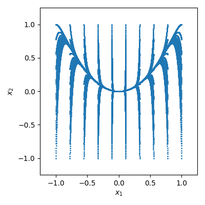
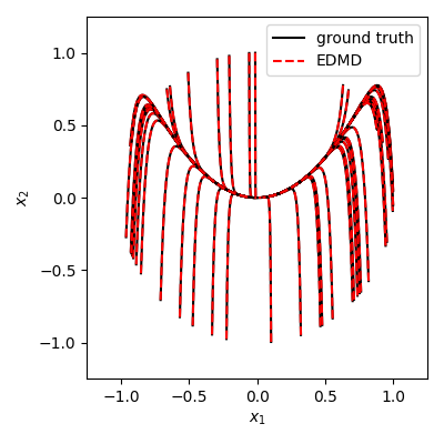
Figure 4: Demonstration on the slow manifold problem. Left: measurement data simulated using the slow manifold in eq. 10. Right: Trajectories of ground truth and predictions from EDMD implemented in PyKoopman given unseen initial conditions.

The PyKoopman package is built around the Koopman class, which approximates the discrete-time Koopman operator from data. To begin, we can create an observable function and an appropriate regressor. These two objects will then serve as input for the Koopman class. For instance, we can employ EDMD to approximate the slow manifold dynamics as shown in eq. 10.

⬇

from pykoopman import Koopman

from pykoopman.observables import Polynomial

from pykoopman.regression import EDMD

model = Koopman(observables=Polynomial(2),regressor=EDMD())

model.fit(X,Xnext)

Once the Koopman object has been fit, we can use the model.simulate method to make predictions over an arbitrary time horizon. For example, the following code demonstrates the usage of model.simulate to make predictions for 50 unseen initial conditions sampled on the unit circle.

⬇

plt.figure(figsize=(4,4))

theta = np.random.rand(1, 50)^∗2^∗np.pi

x0_test_array = np.stack((np.cos(theta), np.sin(theta)),axis=0).T

for x0_test in x0_test_array:

xtest_true = odeint(slow_manifold, x0_test.flatten(), t)

xtest_pred = model.simulate(x0_test,n_steps=t.size-1)

xtest_pred = np.vstack([xtest_true[0], xtest_pred])

plt.plot(xtest_true[:,0], xtest_true[:,1],’k’)

plt.plot(xtest_pred[:,0], xtest_pred[:,1],’r--’)

plt.xlabel(r’$x_1$’)

plt.ylabel(r’$x_2$’)

Figure 4 displays the excellent agreement between ground truth and the EDMD prediction from the aforementioned Koopman model on randomly generated unseen test data. The official GitHub repository contains additional useful examples.

5 Practical tips

In this section, we offer practical guidance for using PyKoopman effectively. We discuss potential pitfalls and suggest strategies to overcome them.

5.1 Observables selection

The use of nonlinear observables makes the approximation of the Koopman operator fundamentally different from DMD. However, choosing observables in practice can be a highly non-trivial task. Although we used monomials as observables in the previous example, such polynomial features are not scalable for practical systems in robotics or fluid dynamics. As a rule of thumb in practice, one can try the thin-plate radial basis function [12] as a first choice. If the number of data snapshots in time is only a few hundred (e.g., as in fluid dynamics), one can opt for kernel DMD [43], but tuning the hyperparameters within the kernel function can be critical. If the number of data points exceeds a few thousand (e.g., multiple trajectories of simulated robotic systems), one can choose to approximate the kernel method with random Fourier features in observables.RandomFourierFeatures as observables [52].

Another useful approach is time-delay observables [13], which can be interpreted as using the reverse flow map function recursively as observables. However, it does not self-start. Just like autoregressive models, the number of delays determines the maximum number of linearly superposable modes that the model can capture. The number of delays also has a somewhat surprising effect on the numerical condition [70].

Furthermore, one may find it beneficial to use customized observables informed by the governing equation in eq. 2 [71] by calling observables.CustomObservables with lambda functions. If all the above methods fail, one may choose to use a neural network to search for the observables; this approach is typically more expressive but is also more computationally expensive.

5.2 Optimization

Once the observables are chosen, the optimization step finds the best-fit linear operator that maps observable at the current time step to the next time step. Although most of the time the standard least-squares regression or pseudo-inverse is sufficient, one can use any regressor from PyDMD. Additionally, one can use NNDMD to concurrently search for the observables and optimal linear fit.

Regarding NNDMD, we have found that using the recurrent loss leads to more accurate and robust model performance than the standard one-step loss, which is adopted in more traditional algorithms. Thanks to the dynamic graph in PyTorch, NNDMD can minimize the recurrent loss progressively, starting from minimizing only the one future step loss to multiple steps in the future. Moreover, we have found that using second-order optimization algorithms, such as L-BFGS [72], significantly accelerates training compared to the Adam optimizer [73]. However, occasionally the standard L-BFGS can diverge, especially when trained over a long period of time. With PyTorch.Lightning, NNDMD can easily take advantage of the computing power of various hardware platforms.

6 Extensions

In this section, we list potential extensions and enhancements to our PyKoopman implementation. We provide references for the improvements that are inspired by previously conducted research and the rationale behind the other potential changes.

• Bilinearization: Although ideally we would like to have a standard linear input-output system in the transformed coordinates, this can lead to inconsistencies with the original system. A number of studies [31, 74, 75] have shown the advantages of using bilinearization instead of standard linearization. It is worth noting that bilinearization has been incorporated into another Python package, pykoop [76].

• Continuous spectrum: Most existing algorithms assume a discrete, pointwise spectrum reflected in the data. As a result, these algorithms may struggle with chaotic systems, which contain a continuous spectrum. There are several approaches for handling continuous spectra, including the use of time delay coordinates [13]. Recent approaches including resDMD, MP-EDMD, and physics informed DMD all show promise for continuous-spectrum dynamics [77, 78, 79].

• Extended libraries: The linear system identified in the lifted space can be further exploited to facilitate the design of optimal control for nonlinear systems. For example, the classic LQR has been extended to nonlinear systems [47]. Moreover, nonlinear MPC can be converted to linear MPC using the identified linear system from the Koopman operator, which transforms the original non-convex optimization problem into a convex optimization problem. In the future, we believe open-source libraries for Koopman-based control synthesis integrated with PyKoopman will be widely used by the community.

7 Acknowledgments

The authors would like to acknowledge support from the National Science Foundation AI Institute in Dynamic Systems (Grant No. 2112085) and the Army Research Office (W911NF-17-1-0306 and W911NF-19-1-0045).

Appendix A Koopman operator theory

In this section, we will briefly describe Koopman operator theory for dynamical systems [4]. Specifically, the theory for autonomous dynamical systems is presented in section A.1 while the theory for controlled systems is presented in section A.2.

A.1 Koopman operator theory for dynamical systems

Given the following continuous-time dynamical system,

$$\frac{d}{dt}\mathbf{x}(t)=\mathbf{f}(\mathbf{x}(t)),$$ (11)

the flow map operator, or time-$t$ map, $\mathbf{F}^{t}:\mathcal{M}\to\mathcal{M}$ maps initial conditions $\mathbf{x}(0)$ to points on the trajectory $t$ time units in the future, so that trajectories evolve according to $\mathbf{x}(t)=\mathbf{F}^{t}(\mathbf{x}(0))$.

The Koopman operator $\mathcal{K}^{t}:\mathcal{G}(\mathcal{M})\mapsto\mathcal{G}(\mathcal{M})$ maps the measurement function $g\in\mathcal{G}(\mathcal{M})$ evaluated at a point $\mathbf{x}(t_{0})$ to the same measurement function evaluated at a point $\mathbf{x}(t_{0}+t)$:

$$\mathcal{K}^{t}g(\mathbf{x})=g(\mathbf{F}^{t}(\mathbf{x})),$$ (12)

where $\mathcal{G}(\mathcal{M})$ is a set of measurement functions $g:\mathcal{M}\to\mathbb{C}$.

The infinitesimal generator $\mathcal{L}$ of the time-$t$ Koopman operator is known as the Lie operator [80], as it is the Lie derivative of $g$ along the vector field $\mathbf{f}(\mathbf{x})$ when the dynamics is given by eq. 2. This follows from applying the chain rule to the time derivative of $g(\mathbf{x})$:

$$\frac{d}{dt}g(\mathbf{x}(t)) =\nabla g\cdot\dot{\mathbf{x}}(t)=\nabla g\cdot\mathbf{f}(\mathbf{x}(t))=\mathcal{L}g(\mathbf{x}(t)).$$ (13)

In continuous-time, a Lie operator eigenfunction $\varphi(\mathbf{x})$ satisfies

$$\frac{d}{dt}\varphi(\mathbf{x})=\mathcal{L}\varphi(\mathbf{x})=\mu\varphi(\mathbf{x}).$$ (14)

An eigenfunction $\varphi$ of $\mathcal{L}$ with eigenvalue $\mu$ is then an eigenfunction of $\mathcal{K}^{t}$ with eigenvalue ${\lambda^{t}=\exp(\mu t)}$. However, we often take multiple measurements of a system, which we will arrange in a vector $\mathbf{g}$:

$$\mathbf{g}(\mathbf{x})=\begin{bmatrix}g_{1}(\mathbf{x})\\ g_{2}(\mathbf{x})\\ \vdots\\ g_{p}(\mathbf{x})\end{bmatrix}.$$ (15)

The vector of observables, $\mathbf{g}$, can be expanded in terms of a basis of eigenfunctions $\varphi_{j}(\mathbf{x})$:

$$\mathcal{K}^{t}\mathbf{g}(\mathbf{x})=\sum_{j=1}^{\infty}\lambda_{j}^{t}\varphi_{j}(\mathbf{x})\mathbf{v}_{j},$$ (16)

where $\mathbf{v}_{j}:=[\langle\varphi_{j},g_{1}\rangle,\langle\varphi_{j},g_{2}\rangle,\ldots,\langle\varphi_{j},g_{p}\rangle]$ is the $j$-th Koopman mode associated with the eigenfunction $\varphi_{j}$.

For a discrete-time system

$$\mathbf{x}_{k+1}=\mathbf{F}(\mathbf{x}_{k}),$$ (17)

where $\mathbf{x}_{k}=\mathbf{x}(t_{k})=\mathbf{x}(k\Delta t)$, the Koopman operator $\mathcal{K}$ governs the one-step evolution of the measurement function $g$,

$$\mathcal{K}g(\mathbf{x}_{k})=g(\mathbf{F}(\mathbf{x}_{k}))=g(\mathbf{x}_{k+1}).$$ (18)

In this case, a Koopman eigenfunction $\varphi(\mathbf{x})$ corresponding to an eigenvalue $\lambda$ satisfies

$$\varphi(\mathbf{x}_{k+1})=\mathcal{K}\varphi(\mathbf{x}_{k})=\lambda\varphi(\mathbf{x}_{k}).$$ (19)

A.2 Koopman theory for controlled systems

The continuous-time dynamics for a controlled system is given by

$$\frac{d}{dt}\mathbf{x}(t)=\mathbf{f}(\mathbf{x}(t),\mathbf{u}(t)).$$ (20)

Following Proctor et al. [81] and Kaiser et al. [47], instead of the usual state $\mathbf{x}$, we consider measurement functions defined on an extended state $\tilde{\mathbf{x}}=(\mathbf{x},\mathbf{u})$, where the corresponding flow map is $\tilde{\mathbf{F}}^{t}(\mathbf{x},\mathbf{u})=[\mathbf{F}^{t}(\mathbf{x},\mathbf{u}),\bm{\Theta}^{t}(\mathbf{u})]$, and $\bm{\Theta}^{t}(\mathbf{u})$ is the shift map by time $t$ units so that $\bm{\Theta}^{t}(\mathbf{u})(s)=\mathbf{u}(s+t)$.

In summary, the Koopman operator on controlled system governs the measurement function of the extended state,

$$\mathcal{K}^{t}g(\mathbf{x},\mathbf{u})=g(\tilde{\mathbf{F}}^{t}(\mathbf{x},\mathbf{u})).$$ (21)

The corresponding Koopman mode decomposition for a vector of observables,

$$\mathbf{g}(\mathbf{x},\mathbf{u})=\begin{bmatrix}g_{1}(\mathbf{x},\mathbf{u})\\ g_{2}(\mathbf{x},\mathbf{u})\\ \vdots\\ g_{p}(\mathbf{x},\mathbf{u})\end{bmatrix},$$ (22)

can be written as,

$$\mathcal{K}^{t}\mathbf{g}(\mathbf{x},\mathbf{u})=\sum_{j=1}^{\infty}\lambda_{j}^{t}\varphi_{j}(\mathbf{x},\mathbf{u})\mathbf{v}_{j},$$ (23)

where the Koopman eigenfunction is

$$\varphi(\mathbf{x},\mathbf{u},t)=\mathcal{K}^{t}\varphi(\mathbf{x},\mathbf{u})=\lambda\varphi(\mathbf{x},\mathbf{u}).$$ (24)

If the continuous-time controlled system is control-affine,

$$\mathbf{f}(\mathbf{x}(t),\mathbf{u}(t))=\mathbf{f}_{0}(\mathbf{x})+\sum_{i=1}^{q}\mathbf{f}_{i}(\mathbf{x})u_{i},$$ (25)

where $u_{i}$ is $i$th component of input $\mathbf{u}$, then the Lie operator (along the vector field $\mathbf{f}$) on the measurement function $g(\mathbf{x})$ becomes,

$$\mathcal{L}g(\mathbf{x})=\nabla_{\mathbf{x}}g(\mathbf{x})\cdot\dot{\mathbf{x}}=\nabla_{\mathbf{x}}g(\mathbf{x})\cdot\mathbf{f}_{0}(\mathbf{x})+\nabla_{\mathbf{x}}g(\mathbf{x})\cdot\sum\limits_{i=1}^{q}\mathbf{f}_{i}(\mathbf{x})u_{i}.$$ (26)

Similarly, after we define the Lie operator along the vector field $\mathbf{f}_{0}$ as $\mathcal{A}$ and that along $\mathbf{f}_{i}$ as $\mathcal{B}_{i}$, we have the bilinearization for the control-affine system,

$$\frac{\text{d}}{\text{d}t}{g}(\mathbf{x})=\mathcal{A}g(\mathbf{x})+\sum\limits_{i=1}^{q}u_{i}\mathcal{B}_{i}g(\mathbf{x}).$$ (27)

Assuming $\varphi$ is an eigenfunction of $\mathcal{A}$, we have

$$\frac{\text{d}}{\text{d}t}{\varphi}(\mathbf{x})=\mu\varphi(\mathbf{x})+\nabla_{\mathbf{x}}\varphi(\mathbf{x})\cdot\sum\limits_{i=1}^{q}\mathbf{f}_{i}(\mathbf{x})u_{i}.$$ (28)

Furthermore, if the vector space spanned by $D$ such eigenfunctions $\{\varphi_{i}\}_{i=1}^{D}$ is invariant under $\mathcal{B}_{1},\ldots,\mathcal{B}_{q}$ [82], we have

$$\forall i=1,\ldots,q,\quad\mathcal{B}_{i}\bm{\varphi}=\mathbf{B}_{i}\bm{\varphi},$$ (29)

where $\bm{\varphi}=\begin{bmatrix}\varphi_{1}&\ldots&\varphi_{D}\end{bmatrix}^{\top}$.

Plugging this into eq. 28, we have the well-known Koopman bilinear form for the control-affine systems,

$$\frac{\text{d}}{\text{d}t}{\bm{\varphi}}(\mathbf{x})=\bm{\Lambda}_{c}\bm{\varphi}(\mathbf{x})+\sum\limits_{i=1}^{q}u_{i}\mathbf{B}_{i}\bm{\varphi}.$$ (30)

For general discrete-time system,

$$\mathbf{x}_{k+1}=\mathbf{F}(\mathbf{x}_{k},\mathbf{u}_{k}),$$ (31)

where $\mathbf{x}_{k}=\mathbf{x}(t_{k})=\mathbf{x}(k\Delta t)$, the Koopman operator governs the one-step evolution of the measurement function $g$ of the extended state $\tilde{x}=(\mathbf{x},\mathbf{u})$,

$$\mathcal{K}g(\mathbf{x}_{k},\mathbf{u}_{k})=g(\mathbf{F}(\mathbf{x}_{k},\mathbf{u}_{k}))=g(\mathbf{x}_{k+1},\mathbf{u}_{k+1}).$$ (32)

A Koopman eigenfunction $\varphi(\mathbf{x})$ corresponding to an eigenvalue $\lambda$ satisfies

$$\varphi(\mathbf{x}_{k+1},\mathbf{u}_{k+1})=\mathcal{K}\varphi(\mathbf{x}_{k},\mathbf{u}_{k})=\lambda\varphi(\mathbf{x}_{k},\mathbf{u}_{k}).$$ (33)

References

- [1] P. J. Schmid, “Dynamic mode decomposition of numerical and experimental data,” Journal of fluid mechanics, vol. 656, pp. 5–28, 2010.
- [2] J. N. Kutz, S. L. Brunton, B. W. Brunton, and J. L. Proctor, Dynamic mode decomposition: data-driven modeling of complex systems. SIAM, 2016.
- [3] P. J. Schmid, “Dynamic mode decomposition and its variants,” Annual Review of Fluid Mechanics, vol. 54, pp. 225–254, 2022.
- [4] S. L. Brunton, M. Budišić, E. Kaiser, and J. N. Kutz, “Modern Koopman theory for dynamical systems,” SIAM Review, vol. 64, no. 2, pp. 229–340, 2022.
- [5] L. Ljung, “Perspectives on system identification,” Annual Reviews in Control, vol. 34, no. 1, pp. 1–12, 2010.
- [6] S. Wright, J. Nocedal et al., “Numerical optimization,” Springer Science, vol. 35, no. 67-68, p. 7, 1999.
- [7] S. L. Brunton and J. N. Kutz, Data-driven science and engineering: Machine learning, dynamical systems, and control. Cambridge University Press, 2022.
- [8] M. Budišić, R. Mohr, and I. Mezić, “Applied Koopmanism,” Chaos: An Interdisciplinary Journal of Nonlinear Science, vol. 22, no. 4, p. 047510, 2012.
- [9] I. Mezić, “Analysis of fluid flows via spectral properties of the Koopman operator,” Annual Review of Fluid Mechanics, vol. 45, pp. 357–378, 2013.
- [10] M. O. Williams, I. G. Kevrekidis, and C. W. Rowley, “A data–driven approximation of the Koopman operator: Extending dynamic mode decomposition,” Journal of Nonlinear Science, vol. 25, no. 6, pp. 1307–1346, 2015.
- [11] S. Klus, F. Nüske, P. Koltai, H. Wu, I. Kevrekidis, C. Schütte, and F. Noé, “Data-driven model reduction and transfer operator approximation,” Journal of Nonlinear Science, vol. 28, no. 3, pp. 985–1010, 2018.
- [12] Q. Li, F. Dietrich, E. M. Bollt, and I. G. Kevrekidis, “Extended dynamic mode decomposition with dictionary learning: A data-driven adaptive spectral decomposition of the Koopman operator,” Chaos: An Interdisciplinary Journal of Nonlinear Science, vol. 27, no. 10, p. 103111, 2017.
- [13] S. L. Brunton, B. W. Brunton, J. L. Proctor, E. Kaiser, and J. N. Kutz, “Chaos as an intermittently forced linear system,” Nature communications, vol. 8, no. 1, pp. 1–9, 2017.
- [14] O. Nelles, “Nonlinear dynamic system identification,” in Nonlinear System Identification. Springer, 2020, pp. 831–891.
- [15] C. W. Rowley, I. Mezić, S. Bagheri, P. Schlatter, and D. S. Henningson, “Spectral analysis of nonlinear flows,” Journal of fluid mechanics, vol. 641, pp. 115–127, 2009.
- [16] H. Akaike, “Fitting autoregressive models for prediction,” Annals of the institute of Statistical Mathematics, vol. 21, no. 1, pp. 243–247, 1969.
- [17] S. A. Billings, Nonlinear system identification: NARMAX methods in the time, frequency, and spatio-temporal domains. John Wiley & Sons, 2013.
- [18] Z. Long, Y. Lu, X. Ma, and B. Dong, “Pde-net: Learning pdes from data,” in International Conference on Machine Learning. PMLR, 2018, pp. 3208–3216.
- [19] L. Yang, D. Zhang, and G. E. Karniadakis, “Physics-informed generative adversarial networks for stochastic differential equations,” SIAM Journal on Scientific Computing, vol. 42, no. 1, pp. A292–A317, 2020.
- [20] C. Wehmeyer and F. Noé, “Time-lagged autoencoders: Deep learning of slow collective variables for molecular kinetics,” The Journal of chemical physics, vol. 148, no. 24, p. 241703, 2018.
- [21] A. Mardt, L. Pasquali, H. Wu, and F. Noé, “Vampnets for deep learning of molecular kinetics,” Nature communications, vol. 9, no. 1, pp. 1–11, 2018.
- [22] P. R. Vlachas, W. Byeon, Z. Y. Wan, T. P. Sapsis, and P. Koumoutsakos, “Data-driven forecasting of high-dimensional chaotic systems with long short-term memory networks,” Proceedings of the Royal Society A: Mathematical, Physical and Engineering Sciences, vol. 474, no. 2213, p. 20170844, 2018.
- [23] J. Pathak, B. Hunt, M. Girvan, Z. Lu, and E. Ott, “Model-free prediction of large spatiotemporally chaotic systems from data: A reservoir computing approach,” Physical review letters, vol. 120, no. 2, p. 024102, 2018.
- [24] L. Lu, X. Meng, Z. Mao, and G. E. Karniadakis, “Deepxde: A deep learning library for solving differential equations,” SIAM Review, vol. 63, no. 1, pp. 208–228, 2021.
- [25] M. Raissi, P. Perdikaris, and G. E. Karniadakis, “Physics-informed neural networks: A deep learning framework for solving forward and inverse problems involving nonlinear partial differential equations,” Journal of Computational Physics, vol. 378, pp. 686–707, 2019. [Online]. Available: https://www.sciencedirect.com/science/article/pii/S0021999118307125
- [26] K. Champion, B. Lusch, J. N. Kutz, and S. L. Brunton, “Data-driven discovery of coordinates and governing equations,” Proceedings of the National Academy of Sciences, vol. 116, no. 45, pp. 22 445–22 451, 2019.
- [27] M. Raissi, A. Yazdani, and G. E. Karniadakis, “Hidden fluid mechanics: Learning velocity and pressure fields from flow visualizations,” Science, vol. 367, no. 6481, pp. 1026–1030, 2020.
- [28] M. Raissi, H. Babaee, and G. E. Karniadakis, “Parametric gaussian process regression for big data,” Computational Mechanics, vol. 64, pp. 409–416, 2019.
- [29] P. Benner, S. Gugercin, and K. Willcox, “A survey of projection-based model reduction methods for parametric dynamical systems,” SIAM review, vol. 57, no. 4, pp. 483–531, 2015.
- [30] B. Peherstorfer and K. Willcox, “Data-driven operator inference for nonintrusive projection-based model reduction,” Computer Methods in Applied Mechanics and Engineering, vol. 306, pp. 196–215, 2016.
- [31] E. Qian, B. Kramer, B. Peherstorfer, and K. Willcox, “Lift & learn: Physics-informed machine learning for large-scale nonlinear dynamical systems,” Physica D: Nonlinear Phenomena, vol. 406, p. 132401, 2020.
- [32] D. Giannakis and A. J. Majda, “Nonlinear laplacian spectral analysis for time series with intermittency and low-frequency variability,” Proceedings of the National Academy of Sciences, vol. 109, no. 7, pp. 2222–2227, 2012.
- [33] O. Yair, R. Talmon, R. R. Coifman, and I. G. Kevrekidis, “Reconstruction of normal forms by learning informed observation geometries from data,” Proceedings of the National Academy of Sciences, vol. 114, no. 38, pp. E7865–E7874, 2017.
- [34] J. Bongard and H. Lipson, “Automated reverse engineering of nonlinear dynamical systems,” Proceedings of the National Academy of Sciences, vol. 104, no. 24, pp. 9943–9948, 2007.
- [35] M. Schmidt and H. Lipson, “Distilling free-form natural laws from experimental data,” science, vol. 324, no. 5923, pp. 81–85, 2009.
- [36] B. C. Daniels and I. Nemenman, “Automated adaptive inference of phenomenological dynamical models,” Nature communications, vol. 6, no. 1, pp. 1–8, 2015.
- [37] S. L. Brunton, J. L. Proctor, and J. N. Kutz, “Discovering governing equations from data by sparse identification of nonlinear dynamical systems,” Proceedings of the National Academy of Sciences, vol. 113, no. 15, pp. 3932–3937, 2016.
- [38] S. H. Rudy, S. L. Brunton, J. L. Proctor, and J. N. Kutz, “Data-driven discovery of partial differential equations,” Science Advances, vol. 3, no. e1602614, 2017.
- [39] M. O. Williams, C. W. Rowley, and I. G. Kevrekidis, “A kernel approach to data-driven Koopman spectral analysis,” Journal of Computational Dynamics, vol. 2, pp. 247–265, 2015.
- [40] B. Lusch, J. N. Kutz, and S. L. Brunton, “Deep learning for universal linear embeddings of nonlinear dynamics,” Nature communications, vol. 9, no. 1, p. 4950, 2018.
- [41] S. E. Otto and C. W. Rowley, “Linearly recurrent autoencoder networks for learning dynamics,” SIAM Journal on Applied Dynamical Systems, vol. 18, no. 1, pp. 558–593, 2019.
- [42] N. Takeishi, Y. Kawahara, and T. Yairi, “Learning koopman invariant subspaces for dynamic mode decomposition,” in Advances in Neural Information Processing Systems, 2017, pp. 1130–1140.
- [43] S. Pan, N. Arnold-Medabalimi, and K. Duraisamy, “Sparsity-promoting algorithms for the discovery of informative Koopman-invariant subspaces,” Journal of Fluid Mechanics, vol. 917, p. A18, 2021.
- [44] A. Surana and A. Banaszuk, “Linear observer synthesis for nonlinear systems using Koopman operator framework,” IFAC-PapersOnLine, vol. 49, no. 18, pp. 716–723, 2016.
- [45] M. Korda and I. Mezić, “Optimal construction of Koopman eigenfunctions for prediction and control,” IEEE Transactions on Automatic Control, vol. 65, no. 12, pp. 5114–5129, 2020.
- [46] A. Mauroy, Y. Susuki, and I. Mezić, Koopman operator in systems and control. Springer, 2020.
- [47] E. Kaiser, J. N. Kutz, and S. L. Brunton, “Data-driven discovery of Koopman eigenfunctions for control,” Machine Learning: Science and Technology, vol. 2, no. 3, p. 035023, 2021.
- [48] S. Peitz and S. Klus, “Koopman operator-based model reduction for switched-system control of pdes,” Automatica, vol. 106, pp. 184–191, 2019.
- [49] S. Peitz, S. E. Otto, and C. W. Rowley, “Data-driven model predictive control using interpolated koopman generators,” SIAM Journal on Applied Dynamical Systems, vol. 19, no. 3, pp. 2162–2193, 2020.
- [50] B. M. de Silva, K. Champion, M. Quade, J.-C. Loiseau, J. N. Kutz, and S. L. Brunton, “Pysindy: a python package for the sparse identification of nonlinear dynamics from data,” arXiv preprint arXiv:2004.08424, 2020.
- [51] M. Hoffmann, M. Scherer, T. Hempel, A. Mardt, B. de Silva, B. E. Husic, S. Klus, H. Wu, N. Kutz, S. L. Brunton et al., “Deeptime: a python library for machine learning dynamical models from time series data,” Machine Learning: Science and Technology, vol. 3, no. 1, p. 015009, 2021.
- [52] A. M. DeGennaro and N. M. Urban, “Scalable extended dynamic mode decomposition using random kernel approximation,” SIAM Journal on Scientific Computing, vol. 41, no. 3, pp. A1482–A1499, 2019.
- [53] N. Demo, M. Tezzele, and G. Rozza, “Pydmd: Python dynamic mode decomposition,” Journal of Open Source Software, vol. 3, no. 22, p. 530, 2018.
- [54] M. S. Hemati, C. W. Rowley, E. A. Deem, and L. N. Cattafesta, “De-biasing the dynamic mode decomposition for applied Koopman spectral analysis of noisy datasets,” Theoretical and Computational Fluid Dynamics, vol. 31, pp. 349–368, 2017.
- [55] T. Askham and J. N. Kutz, “Variable projection methods for an optimized dynamic mode decomposition,” SIAM Journal on Applied Dynamical Systems, vol. 17, no. 1, pp. 380–416, 2018.
- [56] S. Bagheri, “Koopman-mode decomposition of the cylinder wake,” Journal of Fluid Mechanics, vol. 726, pp. 596–623, 2013.
- [57] K. Taira, S. L. Brunton, S. Dawson, C. W. Rowley, T. Colonius, B. J. McKeon, O. T. Schmidt, S. Gordeyev, V. Theofilis, and L. S. Ukeiley, “Modal analysis of fluid flows: An overview,” AIAA Journal, vol. 55, no. 12, pp. 4013–4041, 2017.
- [58] K. Taira, M. S. Hemati, S. L. Brunton, Y. Sun, K. Duraisamy, S. Bagheri, S. Dawson, and C.-A. Yeh, “Modal analysis of fluid flows: Applications and outlook,” AIAA Journal, vol. 58, no. 3, pp. 998–1022, 2020.
- [59] S. L. Brunton, B. W. Brunton, J. L. Proctor, and J. N. Kutz, “Koopman invariant subspaces and finite linear representations of nonlinear dynamical systems for control,” PloS one, vol. 11, no. 2, p. e0150171, 2016.
- [60] M. Korda and I. Mezić, “Linear predictors for nonlinear dynamical systems: Koopman operator meets model predictive control,” Automatica, vol. 93, pp. 149–160, 2018.
- [61] M. Weissenbacher, S. Sinha, A. Garg, and K. Yoshinobu, “Koopman q-learning: Offline reinforcement learning via symmetries of dynamics,” in International Conference on Machine Learning. PMLR, 2022, pp. 23 645–23 667.
- [62] G. Mamakoukas, M. L. Castano, X. Tan, and T. D. Murphey, “Derivative-based Koopman operators for real-time control of robotic systems,” IEEE Transactions on Robotics, vol. 37, no. 6, pp. 2173–2192, 2021.
- [63] I. Abraham and T. D. Murphey, “Active learning of dynamics for data-driven control using Koopman operators,” IEEE Transactions on Robotics, vol. 35, no. 5, pp. 1071–1083, 2019.
- [64] W. Xiong, M. Ma, P. Sun, and Y. Tian, “KoopmanLab: A pytorch module of Koopman neural operator family for solving partial differential equations,” arXiv preprint arXiv:2301.01104, 2023.
- [65] H. Lange, S. L. Brunton, and J. N. Kutz, “From Fourier to Koopman: Spectral methods for long-term time series prediction,” The Journal of Machine Learning Research, vol. 22, no. 1, pp. 1881–1918, 2021.
- [66] I. Mezić and A. Banaszuk, “Comparison of systems with complex behavior,” Physica D: Nonlinear Phenomena, vol. 197, no. 1-2, pp. 101–133, 2004.
- [67] J. H. Tu, “Dynamic mode decomposition: Theory and applications,” Ph.D. dissertation, Princeton University, 2013.
- [68] J. L. Proctor, S. L. Brunton, and J. N. Kutz, “Dynamic mode decomposition with control,” SIAM Journal on Applied Dynamical Systems, vol. 15, no. 1, pp. 142–161, 2016.
- [69] S. Pan and K. Duraisamy, “Physics-informed probabilistic learning of linear embeddings of nonlinear dynamics with guaranteed stability,” SIAM Journal on Applied Dynamical Systems, vol. 19, no. 1, pp. 480–509, 2020.
- [70] S. Pan and K. Duraisamy, “On the structure of time-delay embedding in linear models of non-linear dynamical systems,” Chaos: An Interdisciplinary Journal of Nonlinear Science, vol. 30, no. 7, p. 073135, 2020.
- [71] J. Ng and H. H. Asada, “Data-driven encoding: A new numerical method for computation of the Koopman operator,” arXiv preprint arXiv:2301.06542, 2023.
- [72] J. Nocedal and S. J. Wright, Numerical optimization. Springer, 1999.
- [73] D. P. Kingma and J. Ba, “Adam: A method for stochastic optimization,” arXiv preprint arXiv:1412.6980, 2014.
- [74] D. Bruder, X. Fu, and R. Vasudevan, “Advantages of bilinear Koopman realizations for the modeling and control of systems with unknown dynamics,” IEEE Robotics and Automation Letters, vol. 6, no. 3, pp. 4369–4376, 2021.
- [75] D. Goswami and D. A. Paley, “Bilinearization, reachability, and optimal control of control-affine nonlinear systems: A Koopman spectral approach,” IEEE Transactions on Automatic Control, vol. 67, no. 6, pp. 2715–2728, 2021.
- [76] S. Dahdah and J. R. Forbes, “decargroup/pykoop,” 2022. [Online]. Available: https://github.com/decargroup/pykoop
- [77] M. J. Colbrook, “The mpedmd algorithm for data-driven computations of measure-preserving dynamical systems,” arXiv preprint arXiv:2209.02244, 2022.
- [78] M. J. Colbrook, L. J. Ayton, and M. Szőke, “Residual dynamic mode decomposition: robust and verified koopmanism,” Journal of Fluid Mechanics, vol. 955, p. A21, 2023.
- [79] P. J. Baddoo, B. Herrmann, B. J. McKeon, J. Nathan Kutz, and S. L. Brunton, “Physics-informed dynamic mode decomposition,” Proceedings of the Royal Society A, vol. 479, no. 2271, p. 20220576, 2023.
- [80] B. O. Koopman, “Hamiltonian systems and transformation in Hilbert space,” Proceedings of the National Academy of Sciences, vol. 17, no. 5, pp. 315–318, 1931.
- [81] J. L. Proctor, S. L. Brunton, and J. N. Kutz, “Generalizing Koopman theory to allow for inputs and control,” SIAM Journal on Applied Dynamical Systems, vol. 17, no. 1, pp. 909–930, 2018.
- [82] S. E. Otto and C. W. Rowley, “Koopman operators for estimation and control of dynamical systems,” Annual Review of Control, Robotics, and Autonomous Systems, vol. 4, pp. 59–87, 2021.