Quantum decay of scalar and vector boson stars and oscillons into gravitons

Abstract

We point out that a soliton such as an oscillon or boson star inevitably decays into gravitons through gravitational interactions. These decay processes exist even if there are no apparent self-interactions of the constituent field, scalar or vector, since they are induced by gravitational interactions. Hence, our results provide a strict upper limit on the lifetime of oscillons and boson stars including the dilute axion star. We also calculate the spectrum of the graviton background from decay of solitons.

1 Introduction

Bosons are ubiquitous in physics beyond the Standard Model. For example, the Peccei-Quinn (PQ) mechanism predicts a pseudo-Nambu-Goldstone boson, the QCD axion Peccei:1977hh ; Peccei:1977ur . There may also exist a large number of axion-like particles in the low-energy effective field theory of the string theory. We generally call them axions for both cases. Even if their interaction rates with other particles are suppressed by a large decay constant, they can be produced via coherent oscillations in the early Universe Preskill:1982cy ; Abbott:1982af ; Dine:1982ah and are a good candidate for dark matter (DM). On another hand, massive vector fields in the dark sector can also be considered as a candidate for DM (see Ref. Antypas:2022asj and references therein). However, the production mechanism of vector DM is non-trivial, and includes the misalignment mechanism Nelson:2011sf ; Arias:2012az (see, however, Ref. Nakayama:2019rhg ; Nakayama:2020rka for its difficulty and Ref. Kitajima:2023fun for a viable scenario), emission from cosmic strings Long:2019lwl ; Kitajima:2022lre , phase transition Nakayama:2021avl , scalar-field dependent gauge kinetic coupling Salehian:2020asa ; Firouzjahi:2020whk , preheating and decay of axion-like particles Agrawal:2018vin ; Dror:2018pdh ; Co:2018lka ; Bastero-Gil:2018uel ; Co:2021rhi ; Kitajima:2023pby , and gravitational production during and after inflation Graham:2015rva ; Ema:2019yrd ; Ahmed:2020fhc ; Nakayama:2020ikz ; Kolb:2020fwh ; Arvanitaki:2021qlj ; Sato:2022jya . The cosmological implications of those bosons are therefore important to understand the consistent scenario of particle physics throughout the history of the Universe.

In cosmology, light bosons are usually produced with extremely large occupancy numbers, which imply the formation of Bose-Einstein condensate Guth:2014hsa . In fact, gravitationally bound clumps, called boson stars or oscillatons Kaup:1968zz ; Ruffini:1969qy ; Colpi:1986ye ; Seidel:1991zh ; Tkachev:1991ka ; Kolb:1993zz ; Kolb:1993hw , are formed via the growth of perturbations during the matter dominated era Schive:2014hza ; Levkov:2018kau ; Widdicombe:2018oeo ; Eggemeier:2019jsu ; Chen:2020cef . In the context of axion cosmology, gravitationally bounded clumps of axion are sometimes called dilute axion stars or axiton Kolb:1993hw ; Braaten:2015eeu ; Braaten:2016dlp ; Visinelli:2017ooc ; Schiappacasse:2017ham . In this paper, we simply call them as boson stars. The formation of such objects is supported by detailed numerical simulations Veltmaat:2018dfz ; Eggemeier:2019jsu ; Chen:2020cef , where it was found that localized objects of scalar fields are formed at the center of DM halo, for the QCD axion and ultralight (string) axion. The configuration and properties of the boson star can be calculated by the approach used in Refs. Chavanis:2011zi ; Chavanis:2011zm (see also Ref. Eby:2018ufi ). The boson star is not completely stable but has a long lifetime in vacuum on cosmological time scales Mukaida:2016hwd ; Braaten:2016dlp ; Visinelli:2017ooc ; Eby:2018ufi . The evaporation and growth of boson stars in the DM halo was investigated in Ref. Chan:2022bkz . Those localized objects may affect the image of gravitational lensing Fujikura:2021omw ; Ellis:2022grh . Those objects are therefore relevant in cosmology, especially when they are dominant components of DM in the Universe.

On the other hand, if the attractive self interaction of the scalar field is stronger than the gravitational interaction, the localized object is called an oscillon or I-ball (or dense axion star when the scalar is axion) Bogolyubsky:1976nx ; Segur:1987mg ; Gleiser:1993pt ; Copeland:1995fq ; Gleiser:1999tj ; Honda:2001xg ; Kasuya:2002zs ; Fodor:2006zs ; Fodor:2008du ; Gleiser:2008ty ; Gleiser:2009ys ; Amin:2010jq ; Amin:2011hj ; Salmi:2012ta ; Saffin:2014yka ; Mukaida:2014oza ; Kawasaki:2015vga . A perturbative expansion in terms of the spatial gradient or binding energy is often used to determine the configuration of oscillons Fodor:2008es , whereas some systematic approaches to calculate the configuration in the non-relativistic effective field theory are also proposed in Refs. Braaten:2016kzc ; Mukaida:2016hwd ; Namjoo:2017nia ; Braaten:2018lmj ; Levkov:2022egq . Those objects are realized by the QCD axion after the QCD phase transition in the post-inflationary PQ symmetry breaking scenario Vaquero:2018tib and in a large misalignment scenario Arvanitaki:2019rax . The inflaton may also form oscillons after inflation, depending on models (see, e.g., Ref. Copeland:2002ku ; Amin:2011hj ). However, the lifetime of oscillons tends to be much shorter than the cosmological time scale. It was noted that the amplitude of the primordial gravitational waves may be enhanced if the oscillons dominate the Universe before they decay Inomata:2019ivs ; Lozanov:2022yoy . Therefore, determining the lifetime of those localized objects has important implications for cosmological observations.

Recently, the formation of similar extended objects from vector bosons, which we call the vector boson star or the vector oscillon depending on the attractive force that stabilizes the configuration, has been discussed Adshead:2021kvl ; Jain:2021pnk ; Zhang:2021xxa ; Amin:2023imi . Detailed numerical simulations Gorghetto:2022sue ; Amin:2022pzv ; Jain:2023ojg supports the formation of vector boson stars. They may also have lots of phenomenological impacts, and it is important to understand the stability of these objects.

The classical/quantum stability of the boson star or the oscillon is extensively studied in the literature. In Refs. Mukaida:2016hwd ; Eby:2018ufi , a diagrammatic technique to calculate the classical decay rate of oscillons and axion stars was developed. The resulting decay rate is consistent with that of numerical simulations of oscillons Salmi:2012ta ; Mukaida:2016hwd . See also Refs. Eby:2015hyx ; Eby:2017azn ; Ibe:2019vyo ; Ibe:2019lzv ; Zhang:2020bec ; Zhang:2020ntm for the analysis of the oscillon decay, which agrees with Refs. Mukaida:2016hwd ; Eby:2018ufi and a similar formula was derived there from different perspectives. In Refs. Grandclement:2011wz ; Fodor:2009kg ; Page:2003rd , they considered the classical decay rate of oscillatons. In particular, the dilute axion star is expected to have a very long lifetime. In Ref. Zhang:2020ntm ; Eby:2020ply , they discussed the effect of gravity on the classical decay rate of axion stars.

On the other hand, the quantum decay of oscillons and axion stars was considered in Refs. Hertzberg:2010yz ; Kawasaki:2013awa ; Braaten:2016dlp ; Hertzberg:2018zte with and without parametric resonance. Those works particularly considered the decay into generic scalar fields or photons. The quantum decay process corresponds to the imaginary part of the loop diagrams in the above diagrammatic technique.

In this paper, we consider the quantum decay of soitons, which collectively represent scalar/vector boson stars and oscillons, into gravitons via gravitational interactions. Although a soliton is spherically symmetric, it can produce gravitons (or gravitational waves) quantum mechanically. This is similar to the graviton emission from the spherically symmetric black holes via Hawking radiation, which is a semi-classical process and is classically forbidden. The quantum decay into graviton is inevitable even if the boson has only the quadratic potential. A free real scalar field is the simplest model of quantum field theory but is non-trivial due to the gravitational interactions, where it is localized by its self gravitational potential and decays into gravitons.

Gravitational particle production due to an oscillating scalar field in a cosmological setup has been discussed in Ref. Ema:2015dka , which is also interpreted as the gravitational annihilation of the scalar field into any field. Later this and related subjects have been studied in many papers in the context of dark matter production and reheating Ema:2015dka ; Ema:2016hlw ; Tang:2017hvq ; Ema:2018ucl ; Chung:2018ayg ; Ema:2019yrd ; Mambrini:2021zpp ; Basso:2021whd ; Clery:2021bwz ; Haque:2021mab , graviton production Ema:2015dka ; Schiappacasse:2016nei ; Ema:2016hlw ; Ema:2020ggo , gravitational annihilation of Standard Model particles in thermal bath Garny:2015sjg ; Tang:2016vch ; Tang:2017hvq ; Garny:2017kha ; Gross:2020zam . With this knowledge, it is not surprising that the oscillating scalar field inside the soliton leads to the production of any particle through the gravitational process like $\phi\phi\to XX$, where $\phi$ is a scalar or vector that constitutes the soliton and $X$ denotes any light field since they are inevitably coupled to $\phi$ through gravity. In practice, production of fermions and massless vector bosons are suppressed and dominant process is that into the graviton pair or the Higgs boson (or longitudinal gauge boson) pair if $\phi$ is heavier than them. In particular, the graviton production process is always present no matter how $\phi$ is light. Thus this process provides a strict upper limit on the lifetime of solitons. We stress that this process is inevitable even if there is no explicit scalar self-interaction term in the action. We estimate the graviton production rate by deriving the graviton equation of motion under the scalar/vector soliton background and finding that it is the same as the Mathieu equation. The source of the oscillating term is identified with the oscillating gravitational potential in the presence of soliton.

To the best of our knowledge, the only previous work that explicitly pointed out the quantum graviton production from the scalar oscillon or boson star is Ref. Page:2003rd . There the graviton production rate is calculated by interpreting it as the annihilation process $\phi\phi\to hh$, where $h$ denotes the graviton. In this paper we estimate the graviton production rate by using the time-dependent gravitational potential with the classical soliton configuration. Our approach is useful for more general objects such as Q-balls Coleman:1985ki , vector boson stars or vector oscillons, since in these multi-field solitons it is sometimes nontrivial whether such a perturbative annihilation picture is applicable or not Page:2003rd . In particular, we will see an example in which even the graviton production is absent and our formulation makes it clear.

This paper is organized as follows. In Sec. 2 we briefly review properties of scalar solitons, i.e. oscillons/boson stars for a scalar field, and estimate the time-dependence of the gravitational potential. In Sec. 3 we discuss the case of vector solitons. In Sec. 4 we estimate the gravitational quantum decay rate of a scalar/vector soliton, by using the information on the gravitational potential derived in preceding sections. In Sec. 5 we point out several phenomenological impacts. Sec. 6 is devoted to conclusions and discussion.

2 Scalar solitons

We mainly focus on a spherically symmetric localized configuration of a free real scalar or vector field with gravity, which is sometimes called a boson star. In the context of axion, this corresponds to a dilute axion star. Our qualitative result for quantum decay rate can be applied to almost any localized scalar-field configurations, including oscillons and axion stars. For concreteness, we mainly consider boson stars in this paper and briefly comment on the case of oscillons. We consider a scalar field in this section and a vector field in Sec. 3.

2.1 Setup

We consider a system with the action of

$$S=\int\sqrt{-g}\,d^{4}x\left[-\frac{1}{16\pi G}R+\frac{1}{2}g^{\mu\nu}\partial_{\mu}\phi\partial_{\nu}\phi-V(\phi)\right]\,,$$ (1)

where $R$ is the Ricci scalar, $g$ is the determinant of the metric, $G$ ($=(8\pi M_{\rm Pl}^{2})^{-1}$) is the gravitational constant, and $M_{\rm Pl}$ is the reduced Planck mass. The scalar potential is given by

$$V(\phi) = \frac{1}{2}m^{2}\phi^{2}-\frac{1}{24}\lambda\phi^{4}+\dots\,,$$ (2)

where $m$ is the scalar mass and $\lambda$ is a quartic coupling. We consider the case with a sufficiently small $\lambda$. For the case of axion with a sine-Gordon potential, one can identify $\lambda=m^{2}/f_{a}^{2}$ with $f_{a}$ being the axion decay constant, neglecting higher-dimensional terms.

The gravitational interaction is a long-range force, whereas the self-interaction is a point interaction. The former one can be dominant to determine the localized configuration, if the density at the center of the boson star is sufficiently low. The extent to which this approximation is valid can be understood by estimating the gradient energy, the gravitational potential energy, and the potential energy of the self-interaction,

$$\delta_{x}\sim\frac{\left(\nabla\phi\right)^{2}}{m^{2}\phi^{2}}\sim\frac{1}{(mR)^{2}}\,,$$ (3)

$$\delta_{g}\sim\frac{1}{M_{\rm Pl}^{2}}\int d^{3}x\frac{m^{2}\phi^{2}}{r}\sim\frac{m^{2}\phi^{2}}{M_{\rm Pl}^{2}}R^{2}\,,$$ (4)

$$\delta_{\phi}\sim\frac{\lambda\phi^{4}}{m^{2}\phi^{2}}\,,$$ (5)

where we have normalized the energy densities by $m^{2}\phi^{2}$, $R$ represents the typical size of the boson star and $\phi$ represents the boson field value at the center of boson star. The self-interaction is negligible if $\delta_{g}\gg\delta_{\phi}$. In this case, the size of boson star is determined by $\delta_{x}\sim\delta_{g}$ and we obtain $R\sim(M_{\rm Pl}/\phi)^{1/2}/m$. Using this relation, the consistency condition for this approximation, $\delta_{g}\gg\delta_{\phi}$, is written as

$$\lambda\ll\frac{m^{4}R^{2}}{M_{\rm Pl}^{2}}\sim\frac{m^{2}}{\phi M_{\rm Pl}}\,.$$ (6)

For the case of axion, this condition implies

$$f_{a}\gg\sqrt{\phi M_{\rm Pl}}\,.$$ (7)

We assume that those conditions are met when we discuss boson stars.

Since the gravitational interaction is important, we write the metric around the boson star such as

$$\mathrm{d}s^{2}=e^{-2\Psi(t,r)}\,\mathrm{d}t^{2}-e^{2\Phi(t,r)}\left[\mathrm{d}r^{2}+r^{2}\left(\mathrm{d}\theta^{2}+\sin^{2}\theta\,\mathrm{d}\varphi^{2}\right)\right]\,.$$ (8)

Here, we adopt the isotropic coordinates, which should not be confused with the spherical coordinates Friedberg:1986tp . The energy-momentum tensor is written as

$$T_{\mu\nu} =\partial_{\mu}\phi\partial_{\nu}\phi-\frac{1}{2}g_{\mu\nu}g^{\rho\sigma}\partial_{\rho}\phi\partial_{\sigma}\phi+g_{\mu\nu}V(\phi)\,,$$ (9)

where $V(\phi)\simeq\frac{1}{2}m^{2}\phi^{2}$.

2.2 Configuration of scalar boson star

The Einstein equations read

$$\displaystyle{G^{0}}_{0}=-e^{-2\Phi}\left[2\frac{\partial^{2}\Phi}{\partial r^{2}}+\frac{1}{r}\left(4+r\frac{\partial\Phi}{\partial r}\right)\frac{\partial\Phi}{\partial r}\right]+3e^{2\Psi}\dot{\Phi}^{2}=\frac{\rho}{M_{\rm Pl}^{2}},$$ (10)

$$\displaystyle{G^{0}}_{r}=-2e^{2\Psi}\left(\frac{\partial\Psi}{\partial r}\dot{\Phi}+\frac{\partial\dot{\Phi}}{\partial r}\right)=\frac{e^{2\Psi}}{M_{\rm Pl}^{2}}\frac{\partial\phi}{\partial t}\frac{\partial\phi}{\partial r},$$ (11)

$$\displaystyle{G^{r}}_{r}=e^{-2\Phi}\left[\frac{2}{r}\frac{\partial\Psi}{\partial r}-\frac{2}{r}\frac{\partial\Phi}{\partial r}+2\frac{\partial\Psi}{\partial r}\frac{\partial\Phi}{\partial r}-\left(\frac{\partial\Phi}{\partial r}\right)^{2}\right]+e^{2\Psi}\left(3\dot{\Phi}^{2}+2\dot{\Phi}\dot{\Psi}+2\ddot{\Phi}\right)=-\frac{p_{r}}{M_{\rm Pl}^{2}}\,.$$ (12)

The energy density and pressure are defined as

$$\displaystyle\rho\equiv{T^{0}}_{0}=\frac{e^{2\Psi}}{2}\dot{\phi}^{2}+\frac{e^{-2\Phi}}{2}\left(\frac{\partial\phi}{\partial r}\right)^{2}+\frac{1}{2}m^{2}\phi^{2}\,,$$ (13)

$$\displaystyle p_{r}\equiv-{T^{r}}_{r}=\frac{e^{2\Psi}}{2}\dot{\phi}^{2}+\frac{e^{-2\Phi}}{2}\left(\frac{\partial\phi}{\partial r}\right)^{2}-\frac{1}{2}m^{2}\phi^{2}\,,$$ (14)

where we have used $V(\phi)\simeq\frac{1}{2}m^{2}\phi^{2}.$

We are interested in the weak gravity limit, where we can treat the gravity as perturbations. We thus write $e^{-2\Psi}\simeq 1-2\Psi(t,r)$ and $e^{2\Phi}\simeq 1+2\Phi(t,r)$ and treat $\Psi$ and $\Phi$ as small parameters. From the Einstein equation, they obey

$$\Psi(t,r)=G\int_{r}^{\infty}\frac{\mathrm{d}r^{\prime}}{r^{\prime 2}}\left(M(r^{\prime})+4\pi r^{\prime 3}p_{r}(t,r^{\prime})\right)+\int_{r}^{\infty}\mathrm{d}r^{\prime}\,r^{\prime}\ddot{\Phi}\,,$$ (15)

$$\Phi(t,r)=G\int_{r}^{\infty}\frac{\mathrm{d}r^{\prime}}{r^{\prime 2}}M(r^{\prime})\,,$$ (16)

where

$$M(r)\equiv\int_{0}^{r}dr^{\prime}\,4\pi r^{\prime 2}\rho(r^{\prime})\,,$$ (17)

is the energy enclosed within the radius $r$. As we shall see later, the time dependence of $M(r)$ is negligible for our purpose. Also, while it slowly changes with time via the decay of the scalar field as we will see in Sec. 5, its time scale is much longer. Thus we can neglect $\dot{\Phi}$ to derive the boson star configuration.

The equation of motion for a free scalar field $\phi$ is given by

$$e^{2\Psi}\left[\ddot{\phi}+(\dot{\Psi}+3\dot{\Phi})\dot{\phi}\right]-e^{-2\Phi}\left[\frac{\partial^{2}\phi}{\partial r^{2}}+\frac{2}{r}\frac{\partial\phi}{\partial r}-\left(\frac{\partial\Psi}{\partial r}-\frac{\partial\Phi}{\partial r}\right)\frac{\partial\phi}{\partial r}\right]+\frac{\partial V}{\partial\phi}=0\,.$$ (18)

The scalar field can have a localized configuration thanks to the gravitational attractive interaction. This implies that the spatial gradient energy of the scalar field is proportional to the gravitational potential. We thus neglect the cross term between the spatial gradient and the gravitational potential in the weak gravity limit. Moreover, as we will see shortly, the time-dependent parts of $\Psi$ and $\Phi$ are next-to-leading terms and we can neglect their time derivatives in the equation of motion. We then obtain the simplified equation of motion,

$$(1+2\Psi_{0})\ddot{\phi}-\left(\frac{\partial^{2}\phi}{\partial r^{2}}+\frac{2}{r}\frac{\partial\phi}{\partial r}\right)+m^{2}\phi=0\,,$$ (19)

where we denote the leading-order (time-independent) part of $\Psi$ as $\Psi_{0}$.

Now, let us take an ansatz $\phi(t,r)=\phi_{r}(r)\cos(\omega t)$ to solve the equation of motion. The equation of motion for $\phi_{r}(r)$ is then given by

$$\frac{\partial^{2}\phi_{r}}{\partial r^{2}}+\frac{2}{r}\frac{\partial\phi_{r}}{\partial r}-\left[m^{2}-\omega^{2}(1+2\Psi_{0}(r))\right]\phi_{r}=0\,,$$ (20)

where $\Psi_{0}(r)$ is determined from

$$\frac{1}{4\pi G}\left(\frac{\partial^{2}\Psi_{0}}{\partial r^{2}}+\frac{2}{r}\frac{\partial\Psi_{0}}{\partial r}\right)=-\frac{1}{2}m^{2}\phi_{r}^{2}(r)\,.$$ (21)

To obtain the configuration $\phi_{r}(r)$ through numerical calculations, a convenient approach is to rescale the variables into dimensionless units. The set of equations (20) and (21) can be rewritten as

$$\frac{\partial^{2}\varphi}{\partial z^{2}}+\frac{2}{z}\frac{\partial\varphi}{\partial z}+\left[1-g(z)\right]\varphi=0,$$ (22)

$$\frac{\partial^{2}g}{\partial z^{2}}+\frac{2}{z}\frac{\partial g}{\partial z}=\varphi^{2}(z),$$ (23)

where we define

$$R\equiv\frac{1}{\sqrt{\omega^{2}-m^{2}+2\omega^{2}\Psi_{0}(0)}}\,,$$ (24)

$$r=Rz\,,$$ (25)

$$\phi_{r}(r)=\frac{\varphi(z)}{\sqrt{4\pi G}\,m\omega R^{2}}\,,$$ (26)

$$\Psi_{0}(r)=\Psi_{0}(0)-\frac{g(z)}{2\omega^{2}R^{2}}\,.$$ (27)

Here we note that $\Psi_{0}=0$ at an asymptotic infinity, which implies $g_{\infty}\equiv g(\infty)=2\omega^{2}R^{2}\Psi_{0}(0)$. We numerically solve the above equations from $z=z_{0}\ll 1$ to $z=z_{1}\gg 1$ with the boundary condition of $\varphi(z_{0})=\varphi_{*}$, $\varphi^{\prime}(z_{0})=-\varphi_{*}z_{0}/2$, $g(z_{0})=0$, $g^{\prime}(z_{0})=\varphi_{*}^{2}z_{0}/2$, and $\varphi(\infty)=0$. The localized configuration is realized only by a certain value of $\varphi_{*}$, which can be determined by the shooting algorithm. The result is given by

$$\varphi_{*}\simeq 1.089,$$ (28)

$$g(z\gg 1)\simeq 2.066-\frac{3.619}{z}\,.$$ (29)

In particular, we obtain $g_{\infty}\simeq 2.066$, which implies

$$R\simeq\frac{\sqrt{g_{\infty}-1}}{\epsilon\,m}\simeq\frac{1.0}{\epsilon\,m}\,,$$ (30)

$$\phi_{r}(0)\simeq\frac{0.29\,\epsilon^{2}}{\sqrt{G}}\,,$$ (31)

where we define $\epsilon^{2}\equiv(m^{2}-\omega^{2})/m^{2}$ ($\ll 1$).

We define $R_{99}$ by the radius at which 99% of total energy of the axion star is enclosed. The total energy and $R_{99}$ are given by

$$E\equiv M(\infty)\simeq 1.8\,\frac{\epsilon}{Gm}\,,$$ (32)

$$R_{99}\simeq 5.2\,R\simeq\frac{5.4}{\epsilon\,m}\,.$$ (33)

We note that the amplitude $\phi_{r}(0)$ has to be much larger than $m$, since otherwise the number density is too small for the classical picture to be valid. This requires $\epsilon\gg\sqrt{m/M_{\rm Pl}}$.

2.3 Oscillating behavior of the gravitational potential

Here we derive the the behavior of gravitational potential that helps to understand the quantum decay process. The potential $\Phi$ is given in Eq. (16) as a solution to Eq. (10). To find a time dependence of $\Phi$, it is convenient to look at Eq. (11). By substituting an ansatz for the configuration $\phi(t,r)=\phi_{r}(r)\cos(\omega t)$, it is easy to find that the solution is given in the form of

$$\Phi(t,r)\simeq\Phi_{0}(r)-\frac{\phi_{r}(r)^{2}}{16M_{\rm Pl}^{2}}\cos(2\omega t)\,,$$ (34)

where $\Phi_{0}(r)$ is time-independent part. Parametrically $|\Phi_{0}|\sim(R\omega\phi_{r}/M_{\rm Pl})^{2}$ and it is $(R\omega)^{2}$ times larger than the oscillating term for a typical oscillon radius $R$. As a consistency check, the same expression can be directly derived from (16). To see this, let us note that the energy density $\rho$ satisfies the equation

$$\dot{\rho}=e^{-2\Phi}\left[\frac{1}{r^{2}}\frac{\partial}{\partial r}\left(r^{2}\dot{\phi}\frac{\partial\phi}{\partial r}\right)+\frac{\partial\phi}{\partial r}\left(\dot{\phi}\left(\frac{\partial\Phi}{\partial r}-\frac{\partial\Psi}{\partial r}\right)-\dot{\Phi}\frac{\partial\phi}{\partial r}\right)\right]-e^{2\Psi}3\dot{\Phi}\dot{\phi}^{2}\,.$$ (35)

Neglecting terms involving $\Psi$ or $\Phi$, we find

$$\rho(t,r)\simeq\rho_{0}(r)+\frac{1}{8r^{2}}\frac{\partial}{\partial r}\left(r^{2}\frac{\partial\phi_{r}^{2}}{\partial r}\right)\cos(2\omega t)\,.$$ (36)

By substituting this into Eq. (16) we obtain the same expression as (34). From Eq. (12), we also obtain the time-dependence of $\Psi$ as

$$\Psi(t,r)\simeq\Psi_{0}(r)+\Psi_{1}(r)\cos(2\omega t)\,,$$ (37)

where $|\Psi_{0}|\sim(R\omega\phi_{r}/M_{\rm Pl})^{2}$ and $|\Psi_{1}|\sim(\phi_{r}/M_{\rm Pl})^{2}$. The time dependence of the gravitational potential is essential to understand the quantum decay of the boson star, i.e., the production of gravitationally coupled particles such as gravitons as we will see in Sec. 4.

2.4 The case of complex scalar: Q-balls

Here we give comments on the case of a complex scalar $\phi$ with global U(1) symmetry $\phi\to\phi e^{i\theta}$ with an arbitrary constant $\theta$. The action is

$$S=\int\sqrt{-g}\,d^{4}x\left[-\frac{1}{16\pi G}R+g^{\mu\nu}\partial_{\mu}\phi^{*}\partial_{\nu}\phi-V(|\phi|)\right]\,.$$ (38)

In this case, it is known that there appear soliton-like objects, called Q-balls Coleman:1985ki ; Cohen:1986ct , if the potential is shallower than the quadratic potential. Note that, in contrast to oscillons/I-balls, the potential does not have to be dominated by a quadratic term Kasuya:2002zs . Q-balls are known to play essential roles in the dynamics of supersymmetric flat directions Kusenko:1997ad ; Kusenko:1997zq ; Kusenko:1997si in the context of Affleck-Dine baryogenesis Affleck:1984fy ; Dine:1995kz .

The Q-ball solution is written as $\phi(t,r)=\phi_{r}(r)e^{i\omega t}$ with a real function $\phi_{r}(r)$. A crucial difference from the case of real scalar is that it allows a solution in which the gravitational potential $\Phi$ does not oscillate with time. It is easily seen from the complex scalar version of (11):

$$\displaystyle{G^{0}}_{r}=-2e^{2\Psi}\left(\frac{\partial\Psi}{\partial r}\dot{\Phi}+\frac{\partial\dot{\Phi}}{\partial r}\right)=\frac{e^{2\Psi}}{2M_{\rm Pl}^{2}}\left(\frac{\partial\phi^{*}}{\partial t}\frac{\partial\phi}{\partial r}+\frac{\partial\phi}{\partial t}\frac{\partial\phi^{*}}{\partial r}\right)\,.$$ (39)

For the Q-ball solution, the right hand side is zero and hence the gravitational potential is constant with time. Therefore, no gravitational particle production happens in this limit and such a configuration is stable even against to the graviton production (see Sec. 4). It can be understood as a consequence of the U(1) symmetry and the conserved global charge associated with it. If the orbit is initially elliptical in the complex plane, it will approach to the circular orbit by quantum decay process, including the graviton emission even if there are no explicit U(1) breaking terms.

One may add Planck-suppressed higher-dimensional terms that explicitly break U(1) symmetry. They are motivated by a low-energy effective field theory for quantum gravity, where there should be no global symmetry in nature. Those U(1) symmetry breaking terms distort the dynamics of the complex scalar field from the circular orbit in the complex plane. Then the gravitational potential $\Phi$ has an oscillating term that can result in gravitational emission. As the amplitude of scalar field decreases, the effect of higher-dimensional U(1) breaking terms becomes weaker. Therefore the graviton emission rate becomes smaller as the Q-ball emits more gravitons.

3 Vector solitons

In this section we consider vector solitons and discuss the properties of the gravitational potentials, particularly focusing on their time dependence. While the most discussion is parallel to the case of scalar solitons discussed in the previous section, a crucial difference is that there are polarization degrees of freedom in the case of vector solitons. We follow the analysis in Ref. Adshead:2021kvl (see also Ref. Jain:2021pnk ) and extend it to calculate the time-dependence of gravitational potential.

3.1 Setup

The action we consider is given by

$$S=\int d^{4}x\sqrt{-g}\left[-\frac{R}{16\pi G}-\frac{1}{4}F^{\mu\nu}F_{\mu\nu}+\frac{1}{2}m^{2}A^{\mu}A_{\mu}\right]\,,$$ (40)

where $m$ is the Stuckelberg mass for the dark photon $A^{\mu}$ and $F_{\mu\nu}=\partial_{\mu}A_{\nu}-\partial_{\nu}A_{\mu}$ is its field strength. The energy-momentum tensor is then given by

$$T^{\mu}{}_{\nu}=m^{2}A^{\mu}A_{\nu}-F^{\mu\alpha}F_{\nu\alpha}+\delta^{\mu}_{\nu}\left[-\frac{m^{2}}{2}A_{\alpha}A^{\alpha}+\frac{1}{4}F^{\alpha\beta}F_{\alpha\beta}\right]\,.$$ (41)

The Maxwell equations read

$$\nabla_{\mu}F^{\mu\nu}=\frac{1}{\sqrt{-g}}\partial_{\mu}\left(\sqrt{-g}F^{\mu\nu}\right)=-m^{2}A^{\nu}\,,$$ (42)

where we note that

$$F^{\mu\nu}=g^{\mu\alpha}\left(\partial_{\alpha}A^{\nu}-A_{\beta}\partial_{\alpha}g^{\nu\beta}\right)-g^{\nu\alpha}\left(\partial_{\alpha}A^{\mu}-A_{\beta}\partial_{\alpha}g^{\mu\beta}\right)\,.$$ (43)

This particularly implies the Lorentz condition

$$\nabla_{\nu}A^{\nu}=0\,.$$ (44)

Since we consider a massive gauge field, there are three degrees of freedom for the gauge field and $A^{0}$ is a non-dynamical field.

We are interested in the weak-gravity limit, where the metric is treated as a perturbation from the Minkowski metric. In the Newtonian gauge, we write

$$ds^{2}=(1-2\Psi)d\tau^{2}+2V_{i}dx^{i}d\tau-\left[(1+2\Phi)\delta_{ij}-h_{ij}\right]dx^{i}dx^{j}\,,$$ (45)

where $\partial_{i}V_{i}=0$ and we also choose a gauge to eliminate the transverse vector degree of freedom. The transverse-traceless metric perturbation $h_{ij}$ satisfies $\partial_{i}h_{ij}=\partial_{i}h_{ji}=0$, and $h_{ii}=0$. This completely fixes the gauge: $\Psi$, $\Phi$ and $V_{i}$ are given in terms of $A_{\mu}$. We first neglect $h_{ij}$ to determine the profile of vector star and later take it into account to discuss the quantum decay. In particular, we have

$$\sqrt{-g}=1+(3\Phi-\Psi)\,,$$ (46)

for $h_{ij}=0$.

3.2 Configuration of vector boson star

The Lorentz constraint Eq. (44) is written as

$$\partial_{0}A^{0}+\partial_{i}A^{i}+A^{0}\partial_{0}\left(3\Phi-\Psi\right)+A^{j}\partial_{j}(3\Phi-\Psi)=0\,.$$ (47)

We are interested in the mode that oscillates with a frequency of $\omega\simeq m$. This implies $A^{0}=\mathcal{O}(A^{i}/(mR))$ at the leading order, where $R$ is the typical size of the object. For $mR\gg 1$, the Maxwell equations and the Lorentz condition are greatly simplified such as

$$\partial_{0}^{2}A^{j}-\Delta A^{j}+\partial_{0}\left(5\Phi+\Psi\right)\partial_{0}A^{j}+\left[(1-2\Psi)m^{2}+2\partial_{0}^{2}\Phi\right]A^{j}\simeq 0\,,$$ (48)

$$\partial_{0}A^{0}+\partial_{i}A^{i}\simeq 0\,,$$ (49)

where $\Delta=\partial_{i}\partial_{j}\delta^{ij}$. Here we included the leading-order terms that has time derivatives of gravitational potentials, which are negligible compared with the other terms, though. The Einstein equation leads to

$$-\Delta\Phi=\frac{1}{2M_{\rm Pl}^{2}}T^{0}{}_{0}\,,$$ (50)

$$-\frac{2}{3}\Delta^{2}(\Psi-\Phi)=\frac{1}{M_{\rm Pl}^{2}}\left[\delta^{il}\delta^{jk}\partial_{i}\partial_{j}-\frac{\delta^{kl}\Delta}{3}\right]T^{k}{}_{l}\,,$$ (51)

$$\Delta V_{i}=\frac{2}{M_{\rm Pl}^{2}}T^{0}{}_{i}^{\rm(T)}\,,$$ (52)

$$-\partial_{i}\dot{\Phi}=\frac{1}{2M_{\rm Pl}^{2}}T^{0}{}_{i}^{\rm(L)}\,,$$ (53)

where the superscript (T) and (L) indicate the transverse and longitudinal component, respectively. Here, the $(0,0)$ and $(0,i)$ component of the energy-momentum tensor are given by

$$T^{0}{}_{0}\simeq\frac{m^{2}}{2}\left(A^{0}\right)^{2}+\frac{m^{2}}{2}\sum_{i}\left(A^{i}\right)^{2}(1+2\Phi)+\frac{1}{2}\sum_{i}(\partial_{0}A^{i})^{2}(1+2\Phi+2\Psi)$$

$$~{}~{}~{}~{}~{}~{}~{}~{}~{}~{}~{}+\sum_{i}\partial_{0}A^{i}\partial_{i}A^{0}+\frac{1}{2}\sum_{i,j}\left(\partial_{i}A^{j}\partial_{i}A^{j}-\partial_{i}A^{j}\partial_{j}A^{i}\right),$$ (54)

$$T^{0}{}_{i}\simeq-m^{2}A^{0}A^{i}-\sum_{j}\partial^{0}A^{j}(\partial_{j}A^{i}-\partial_{i}A^{j})\,,$$ (55)

where we include terms up to $\mathcal{O}(k^{2}(A^{i})^{2})$ for $T^{0}{}_{0}$ and leading-order terms for $T^{0}{}_{i}$.

Now, let us suppose

$$A^{i}=n^{i}f(r)\cos(\omega t+\theta^{i})\,,$$ (56)

where $n_{i}$ is a unit vector representing the polarization and $\theta^{i}$ is the phase. Then, at the leading order, the equation of motion for $f$ is independent of the polarization and is given by

$$\frac{\partial^{2}f}{\partial r^{2}}+\frac{2}{r}\frac{\partial f}{\partial r}-\left[m^{2}-\omega^{2}(1+2\Psi_{0}(r))\right]f=0\,,$$ (57)

where $\Psi_{0}(r)$ is the leading-order term of $\Psi$ and is given by

$$\frac{1}{4\pi G}\left(\frac{\partial^{2}\Psi_{0}}{\partial r^{2}}+\frac{2}{r}\frac{\partial\Psi_{0}}{\partial r}\right)=-\frac{1}{2}m^{2}f^{2}(r)\,.$$ (58)

The latter equation comes from Eq. (50) by noting $\Psi_{0}\simeq\Phi_{0}$ from Eq. (51) at the leading order. These are identical to the equations for the scalar fields (see Eqs. (20) and (21)). So the mass, size, and amplitude at the center of the vector boson star are the same with those for scalar boson star.

3.3 Oscillating behavior of the gravitational potential

Similarly to the case of scalar boson star studied in the previous section, we are interested in the behavior of the gravitational potential $\Psi$ and $\Phi$ and its time dependence since it is essential to evaluate the quantum decay rate. Compared with the scalar case, it is nontrivial since there are four components $A_{\mu}$ and several configurations of the vector polarization are known Adshead:2021kvl ; Jain:2021pnk ; Zhang:2021xxa . Our short conclusion is that in the massive vector case, at least for known configurations, the gravitational potential oscillates with a similar amplitude. In deriving it, $A^{0}$ plays an important role since it is related to $A^{i}$ through the Lorentz constraint (49).

Using the ansatz Eq. (56), we obtain the constraint from the Lorentz condition Eq. (49) such as

$$A^{0}=-\frac{1}{\omega}\sum_{i}n^{i}\partial_{i}f(r)\sin(\omega t+\theta^{i})\,.$$ (59)

Substituting these into $T^{0}{}_{0}$, we obtain

$$T^{0}{}_{0} \simeq\frac{m^{2}}{2\omega^{2}}\left(\sum_{i}n^{i}\partial_{i}f\sin(\omega t+\theta^{i})\right)^{2}+\frac{m^{2}}{2}\sum_{i}\left(n^{i}f(r)\cos(\omega t+\theta^{i})\right)^{2}(1+2\Phi)$$

$$+\frac{\omega^{2}}{2}\sum_{i}(n^{i}f(r)\sin(\omega t+\theta^{i}))^{2}(1+2\Phi+2\Psi)$$

$$+\sum_{i}n^{i}f(r)\sin(\omega t+\theta^{i})\left(\sum_{j}n^{j}\partial_{i}\partial_{j}f\sin(\omega t+\theta^{j})\right)$$

$$+\frac{1}{2}\sum_{i,j}\left(n^{j}n^{j}\partial_{i}f\partial_{i}f\cos^{2}(\omega t+\theta^{j})-n^{i}n^{j}\partial_{i}f\partial_{j}f\cos(\omega t+\theta^{i})\cos(\omega t+\theta^{j})\right)\,.$$

In the following, we consider two extremely polarized configurations to see the time-dependence of gravitational potential.

3.3.1 Linear polarization

Let us consider the case with a linear polarization: $n^{1}=1$, $n^{2}=0$, $n^{3}=0$, $\theta^{i}=0$. We then obtain

$$T^{0}{}_{0} \simeq\frac{1}{2}\hat{x}^{2}(f^{\prime})^{2}\sin^{2}(\omega t)+\frac{m^{2}}{2}(1+2\Phi)f^{2}+\frac{(\omega^{2}-m^{2})+2\omega^{2}\Psi}{2}f^{2}\sin^{2}(\omega t)$$ (61)

$$+f\left(f^{\prime}/r+\hat{x}^{2}(f^{\prime\prime}-f^{\prime}/r)\right)\sin^{2}(\omega t)+\frac{1}{2}f^{\prime 2}(1-\hat{x}^{2})\cos^{2}(\omega t)\,,$$

$$=\frac{m^{2}}{2}(1+2\Phi)f^{2}+\left(-\frac{ff^{\prime\prime}}{2}+\hat{x}^{2}\left(ff^{\prime\prime}+\frac{f^{\prime}f^{\prime}}{2}-\frac{ff^{\prime}}{r}\right)\right)\sin^{2}(\omega t)$$

$$+\frac{1}{2}f^{\prime 2}(1-\hat{x}^{2})\cos^{2}(\omega t)\,,$$

where $\hat{x}\equiv x/r$, the prime denotes the derivative with respect to $r$ and we used Eq. (57) in the last line. The large parenthesis in front of $\sin^{2}(\omega t)$ is given by $\sim f^{2}/R^{2}$ with $R$ being the typical size of the vector boson star. Noting that

$$\Delta f^{2}(r)=2\left(ff^{\prime\prime}+f^{\prime 2}+\frac{2ff^{\prime}}{r}\right)\sim\frac{f^{2}}{R^{2}}\,,$$ (62)

and Eq. (50), we approximate the gravitational potential as

$$\Phi(t,r)\sim\Phi_{0}(r)+\frac{f^{2}}{16M_{\rm Pl}^{2}}\cos(2\omega t)\,,$$ (63)

which should be regarded as an order-of-magnitude estimate. Here, we particularly omit the deviation from the spherical symmetry.

3.3.2 Circular polarization

Let us consider the case with a maximally circular polarization: $n^{1}=1/\sqrt{2}$, $n^{2}=1/\sqrt{2}$, $n^{3}=0$, $\theta^{1}=0$, $\theta^{2}=\mp\pi/2$, $\theta^{3}=0$. We first note that $\sum_{i}n^{i}\partial_{i}f\sin(\omega t+\theta^{i})=f^{\prime}(\hat{x}\sin(\omega t)\mp\hat{y}\cos(\omega t))/\sqrt{2}=f^{\prime}\sin(\omega t\mp\phi_{x})\sin\phi_{z}/\sqrt{2}$, where $x=r\cos\phi_{x}\sin\phi_{z}$ and $y=r\sin\phi_{x}\sin\phi_{z}$. We then obtain

$$T^{0}{}_{0} \simeq\frac{m^{2}}{2}(1+2\Phi)f^{2}+\frac{(\omega^{2}-m^{2})+2\omega^{2}\Psi}{4}f^{2}+\frac{1}{4}f^{\prime}f^{\prime}$$ (64)

$$+\frac{1}{4}\sin^{2}\phi_{z}f^{\prime}f^{\prime}\left(\sin^{2}(\omega t\mp\phi_{x})-\cos^{2}(\omega t\mp\phi_{x})\right)$$

$$+\frac{1}{2}f\left[\partial_{x}^{2}f\sin^{2}(\omega t)\mp 2\partial_{x}\partial_{y}f\cos(\omega t)\sin(\omega t)+\partial_{y}^{2}f\cos^{2}(\omega t)\right].$$

Here, the third line can be rewritten as

$$\frac{1}{2}\left[\frac{ff^{\prime}}{r}+\left(ff^{\prime\prime}-\frac{ff^{\prime}}{r}\right)\sin^{2}(\omega t\mp\phi_{x})\sin^{2}\phi_{z}\right].$$ (65)

Using Eq. (57), we finally obtain

$$T^{0}{}_{0} \simeq\frac{m^{2}}{2}(1+2\Phi)f^{2}+\frac{1}{4}\left(f^{\prime}f^{\prime}-ff^{\prime\prime}\right)-\frac{1}{4}f^{\prime}f^{\prime}\cos^{2}(\omega t\mp\phi_{x})\sin^{2}\phi_{z}$$ (66)

$$+\frac{1}{2}\left(ff^{\prime\prime}+\frac{1}{2}f^{\prime}f^{\prime}-\frac{ff^{\prime}}{r}\right)\sin^{2}(\omega t\mp\phi_{x})\sin^{2}\phi_{z}\,.$$

Thus we have the oscillating term. Again, from Eq. (50), we approximate the gravitational potential as

$$\Phi(t,r)\sim\Phi_{0}(r)+\frac{f^{2}}{16M_{\rm Pl}^{2}}\cos(2\omega t\pm 2\phi_{x})\,.$$ (67)

This should be regarded as an order-of-magnitude estimate because we particularly omit the deviation from the spherical symmetry. This is the same orders-of-magnitude result as the linear polarized case.

4 Quantum decay into gravitons

Now let us estimate the quantum production rate of the graviton in the boson star. As far as we consider the graviton wavelength much shorter than the typical size of the boson star $R$, we can approximate the metric as if it is spatially flat. Then the the equation of motion of the gravitational wave $h_{\lambda}$, with $\lambda=+,\times$ being the polarization, is given by

$$\ddot{h}_{\lambda}+(3\dot{\Phi}+\dot{\Psi})\dot{h}_{\lambda}+e^{-2(\Psi+\Phi)}k^{2}h_{\lambda}=0\,,$$ (68)

where $k$ denotes the wavenumber. One may think that both the oscillating $\Psi$ and $\Phi$ may induce the particle production, but we need to take care of the $e^{-2(\Psi+\Phi)}$ factor in front of the $k^{2}$ term. Actually it turns out that oscillation of $\Psi$ does not lead to particle production. In order to see this, let us define a new time variable $d\tau\equiv e^{-(\Psi+\Phi)}dt$. Then the equation of motion (68) is rewritten as

$$\partial^{2}_{\tau}h_{\lambda}+2(\partial_{\tau}\Phi)(\partial_{\tau}h_{\lambda})+k^{2}h_{\lambda}=0\,.$$ (69)

With this time variable, $\Psi$ disappeared and it is time dependence of $\Phi$ that leads to particle production. This is further simplified by defining $\widetilde{h}_{\lambda}\equiv e^{\Phi}h_{\lambda}$ as

$$\partial^{2}_{\tau}{\widetilde{h}}_{\lambda}+\left(k^{2}-\frac{\partial^{2}_{\tau}b}{b}\right)\widetilde{h}_{\lambda}=0\,,$$ (70)

where $b\equiv e^{\Phi}$. The time-dependent effective mass term is given by

$$\frac{\partial^{2}_{\tau}b}{b}\simeq\left(\frac{\omega\phi_{r}}{2M_{\rm Pl}}\right)^{2}\cos(2\omega t)~{}~{}~{}{\rm for~{}scalar}\,,$$ (71)

$$\frac{\partial^{2}_{\tau}b}{b}\simeq\left(\frac{\omega f}{2M_{\rm Pl}}\right)^{2}\cos(2\omega t)~{}~{}~{}{\rm for~{}vector}\,,$$ (72)

from Eq. (34) for the scalar case. Since the scalar and vector cases give similar results, below we collectively denote by $\phi$ both the scalar and vector boson for notational simplicity.

Equation (70) is the same as the Mathieu equation and hence the modes with $k\simeq\omega$ are enhanced. Once the equation of motion is identified with the Mathieu equation, we can use the same technique to solve this equation (e.g. the Bogoliubov coefficient technique) and derive the production rate in the narrow width limit, as found in literature Dolgov:1989us ; Traschen:1990sw ; Shtanov:1994ce ; Kofman:1997yn . In the case of purely gravitational production, more details are found in Refs. Ema:2015dka ; Ema:2018ucl ; Chung:2018ayg . Although we do not repeat the calculation details here, the point is that it is regarded as a perturbative annihilation of the scalar or vector into the graviton pair $\phi\phi\to hh$, since $(\phi_{r}/2M_{\rm Pl})^{2},(f/2M_{\rm Pl})^{2}\ll 1$. The graviton production rate from a boson star is given by

$$\Gamma_{\rm grav}=\Gamma(\phi\phi\to hh)=\frac{\mathcal{C}}{256\pi}\frac{\phi_{R}^{2}m^{3}}{M_{\rm Pl}^{4}}\,,$$ (73)

where $\phi_{R}$ denotes the typical amplitude of $\phi$ in the scalar boson star or $A_{i}$ in the vector boson star and we approximated $\omega\simeq m$, and $\mathcal{C}$ is an $\mathcal{O}(1)$ coefficient that represents the effect of radial shape of the boson star.

Note that this production mechanism is purely quantum. The production through (70) requires initial seed of the graviton field $\widetilde{h}_{\lambda}$, which is provided by the zero-point fluctuation in the vacuum. Thus it is not understood as a gravitational wave production from classical sources. Although a spherically symmetric boson star cannot be a classical source of gravitational waves, it can enhance the graviton quantum fluctuations existing there.

Here we comment on the possibility of parametric resonance. The equation of motion (70) is exactly the form of the Mathieu equation, and hence one may wonder whether the parametric resonant amplification of the graviton can happen or not. To see this, let us compare the growth rate of the graviton amplitude and the escape rate of the produced graviton from the soliton. If the former is larger than the latter, the parametric resonance can happen. Otherwise gravitons do not accumulate in the phase space with narrow momentum rage around $k\sim\omega$ and no Bose enhancement would be expected Hertzberg:2010yz ; Kawasaki:2013awa . The growth rate is characterized by the parameter $\mu$, which is defined as $h_{\lambda}\propto e^{\mu t}$. In our case it is given by $\mu\sim\omega\phi_{R}^{2}/M_{\rm Pl}^{2}$ Kofman:1997yn . On the other hand, the escape rate is simply given by $\sim 1/R\sim\omega\phi_{R}/M_{\rm Pl}$ for the self-gravitating boson star, which is larger than the growth rate $\mu$. For the oscillon with self-interactions, the escape rate is even larger. Therefore, the escape rate is always larger than the growth rate for $\phi_{R}\ll M_{\rm Pl}$. Thus we conclude that there is no parametric resonance effect and the graviton production rate is linear in time with the perturbative rate (73).

All the Standard Model particles are also gravitationally coupled to $\phi$ and $A^{\mu}$ and hence their pair production can happen through the $s$-channel graviton exchange. Among them, massless fermion and transverse vector boson production are suppressed due to their conformal nature. The production rate of fermions is $(m_{f}/m)^{2}$ times smaller than the graviton production rate, where $m_{f}$ is the fermion mass. On the other hand, scalar production is not suppressed unless it is conformally coupled to the Ricci scalar. The equation of motion of a free scalar $\chi$, which is minimally coupled to gravity, is given by

$$e^{2\Psi}\left[\ddot{\chi}+(3\dot{\Phi}+\dot{\Psi})\dot{\chi}\right]-e^{-2\Phi}\vec{\nabla}^{2}\chi+m_{\chi}^{2}\chi=0\,,$$ (74)

where $m_{\chi}$ is the mass of $\chi$. Similarly to the graviton case, it is simplified by introducing $\widetilde{\chi}\equiv e^{\Phi}\chi$ as

$$\partial^{2}_{\tau}\widetilde{\chi}+\left(k^{2}-\frac{\partial^{2}_{\tau}b}{b}+b^{2}m_{\chi}^{2}\right)\widetilde{\chi}=0\,,$$ (75)

where we have moved to the Fourier space. Therefore, if $k\simeq m\gg m_{\chi}$, the scalar production rate is the same as the graviton production rate up to a factor $2$ coming from the graviton polarization degrees of freedom. In the Standard Model, the production rate of the Higgs boson is the same order of the graviton production rate if $m$ is much larger than the Higgs mass. In the electroweak symmetry breaking phase, the production of longitudinal massive vector bosons is also the same order. If $0.1$ GeV $\lesssim m\lesssim 1$ GeV, the boson stars may also efficiently produce pions or other mesons. If there exist other scalar fields lighter than $\phi$ or $A^{\mu}$, such as axions, they should also be produced with the same production rate.

5 Phenomenological implications of gravitational decay

In this section, we discuss time evolution of the boson star with a gravitational decay rate of (73) and then calculate the spectrum of graviton background. The following discussion applies to the case of both scalar and vector. For notational simplicity we simply express them by $\phi$, but it can be as either scalar or vector.

5.1 Decay of boson star

If there are no direct interactions between $\phi$ (or $A^{\mu}$) and other lighter fields, the gravitational processes are the only processes that cause the decay of boson star. Classical decay processes such as $3\phi\to\phi$ are possible mediated by the gravitational interaction Page:2003rd , but it is likely to be exponentially suppressed for $\omega R\gg 1$. In this limit, the graviton production is an inevitable decay process and it gives a strict lower bound on the lifetime of oscillons/boson stars.

Via the graviton production, a boson star mass $M$ decreases according to

$$\dot{M}(t)=-\Gamma_{\rm grav}(t)M(t)\,.$$ (76)

Note that the decay rate (73) depends on the amplitude of the scalar/vector in the boson star $\phi_{R}$ and hence the decay rate decreases as the boson star mass decreases. By using the relation $M\sim m^{2}\phi_{R}^{2}R^{3}$ and the equilibrium condition $GM\sim(Rm^{2})^{-1}$, we find $\Gamma_{\rm grav}\propto M^{4}$. Then we can solve (76) as

$$M^{4}(t)=\frac{M_{i}^{4}}{1+\Gamma_{\rm grav}^{0}t},~{}~{}~{}~{}~{}~{}~{}~{}~{}\Gamma_{\rm grav}^{0}\equiv\frac{\mathcal{C}}{1024\pi}\frac{\phi_{R,i}^{2}m^{3}}{M_{\rm Pl}^{4}}\,,$$ (77)

where we assumed the initial boson star mass $M_{i}$ in the limit $t\to 0$ and $\phi_{R,i}$ denotes the initial scalar/vector amplitude at the boson star formation. Correspondingly, we obtain

$$\phi_{R}^{2}(t)=\frac{\phi_{R,i}^{2}}{1+\Gamma_{\rm grav}^{0}t}\,.$$ (78)

Therefore, the boson star mass decreases rather slowly as $M\propto t^{-1/4}$ for $t\gtrsim(\Gamma_{\rm grav}^{0})^{-1}$. We call $\tau_{\rm grav}\equiv(\Gamma_{\rm grav}^{0})^{-1}$ as the boson star lifetime, although it does not decay exponentially. Numerically it is estimated as

$$\tau_{\rm grav}=(\Gamma_{\rm grav}^{0})^{-1}\simeq 1\times 10^{16}\,{\rm sec}\,\left(\frac{M_{\rm Pl}}{\phi_{R,i}}\right)^{2}\left(\frac{1\,{\rm GeV}}{m}\right)^{3}\,.$$ (79)

It easily exceeds the present age of the universe for, e.g., light axion-like particles $m\lesssim 1\,{\rm eV}$. If $m>\mathcal{O}(100)$ GeV, the boson stars may efficiently produce the Higgs boson and longitudinal weak bosons after the Big-Bang Nucleosynthesis epoch with a rate similar to the graviton production. This gives a constraint on the abundance of boson star. We will come back to this issue in detail elsewhere.

Once the amplitude $\phi_{R}(t)$ becomes smaller than $m$, the classical picture of the boson star may no longer be valid. This happens at $t\sim\left[\Gamma_{\rm grav}^{0}(m/\phi_{R,i})^{2}\right]^{-1}$. Then one has to treat the bosons as individual particles with negligible Bose enhancement effect.

5.2 Decay of oscillon and Q-ball

Here we comment on the case with oscillon, where the self-interactions support the localized configuration. In most cases, oscillons classically decay into individual particles via self-interactions. In a certain case, however, the classical decay processes mediated by the self-interactions can be exponentially suppressed for $\omega R\gg 1$ Mukaida:2016hwd . In this limit, the graviton production is an inevitable decay process and it gives strict lower bound on the lifetime of oscillon.

The graviton production rate is given by the same formula (73). In order to discuss the evolution of the oscillon, we need to know the relation between $\phi_{R}$ and $R$. It is nontrivial and highly model-dependent. Nevertheless, we can make an orders-of-magnitude estimate for the typical time scale at which the gravitational process becomes important. Independently of the relation between $\phi_{R}$ and $R$, we can repeat a similar procedure to the case of boson star, and find a typical time scale $\tau_{\rm grav}$, the same as (79), although the time dependence of the boson star mass $M(t)$ at $t>\tau_{\rm grav}$ may differ from the boson star case. Thus Eq. (79) gives a reasonable estimate for the oscillon lifetime for $\omega R\gg 1$ when the classical decay processes are exponentially suppressed.

As we discussed in Sec. 2.4, the quantum decay of Q-ball into graviton is forbidden by the conserved global charge for the case with the exactly spherical orbit in the complex plane. If one adds higher-dimensional U(1)-breaking terms, the orbit in the complex plane becomes elliptical and the quantum decay process to the graviton becomes open. The amplitude of scalar field decreases as it decays, which makes decay slower. The resulting time-dependence for the graviton emission rate is different from the case with boson stars and provides an unique signals in gravitational wave spectrum.

Below we estimate the effect of graviton production on the Q-ball. Let us suppose that the orbit of the complex scalar field $\phi$ is given by $\phi(t)=\varphi_{R}\cos(\omega t)+i\varphi_{I}\sin(\omega t)$ inside the Q-ball with $\varphi_{R}$ and $\varphi_{I}$ being the amplitude of the real and imaginary component. Without loss of generality, we take $\varphi_{R}>\varphi_{I}$ initially. From Eq. (39), the gravitational potential $\Phi(t,r)$ is given by

$$\Phi(t,r)\simeq\Phi_{0}(r)-\frac{\varphi_{R}^{2}(t,r)-\varphi_{I}^{2}(t,r)}{16M_{\rm Pl}^{2}}\cos(2\omega t).$$ (80)

Repeating the same discussion for the case of real scalar, we obtain the graviton production rate due to the oscillating gravitational potential as

$$\Gamma_{\rm grav}=\frac{\mathcal{C}}{256\pi}\frac{(\varphi_{R}^{2}-\varphi_{I}^{2})\,\omega^{3}}{M_{\rm Pl}^{4}}.$$ (81)

It is expected that $\varphi_{R}^{2}-\varphi_{I}^{2}$ decreases through the graviton production and this process stops when $\varphi_{R}=\varphi_{I}$. On the other hand, the Q-ball charge $Q$ should be conserved as far as there is no explicit U(1) breaking term. It is roughly estimated as $Q\sim\omega\varphi_{R}\varphi_{I}\times R^{3}\sim\varphi_{R}\varphi_{I}/(\omega^{2}K^{3})$ where we assumed that the Q-ball radius is given by $R\sim 1/(\omega K)$ with some numerical constant $K$. Thus the final value will be $\varphi_{R}=\varphi_{I}\sim\omega\sqrt{K^{3}Q}\equiv\bar{\varphi}$. Keeping this in mind, one can solve (76) in the case of Q-ball.

For $\varphi_{R}\gg\varphi_{I}$, the situation is similar to the case of real scalar. We obtain

$$\varphi_{R}^{2}(t)\simeq\frac{\varphi_{R,i}^{2}}{1+\Gamma^{0}_{\rm grav}t},~{}~{}~{}~{}~{}~{}M(t)\simeq\frac{M_{i}}{1+\Gamma^{0}_{\rm grav}t},~{}~{}~{}~{}~{}~{}\Gamma^{0}_{\rm grav}=\frac{\mathcal{C}}{256\pi}\frac{\varphi_{R,i}^{2}\,\omega^{3}}{M_{\rm Pl}^{4}}.$$ (82)

Note that we have assumed that the Q-ball mass is given by $M\simeq\omega^{2}(\varphi_{R}^{2}+\varphi_{I}^{2})\times R^{3}\sim(\varphi_{R}^{2}+\varphi_{I}^{2})/(\omega K^{3})$. The amplitude $\varphi_{R}$ decreases according to this result. Eventually $\varphi_{R}$ becomes close to $\varphi_{I}$ at $t=\bar{t}$ and the above approximation breaks down. After this epoch, by defining $\varphi_{R}=\bar{\varphi}+\delta\varphi$ and $\varphi_{I}=\bar{\varphi}-\delta\varphi$ and noting that $M\sim(\bar{\varphi}^{2}+\delta\varphi^{2})/(\omega K^{3})$, we obtain

$$\delta\varphi(t)=\delta\varphi(\bar{t})-2\overline{\Gamma}_{\rm grav}\bar{\varphi}(t-\bar{t}),~{}~{}~{}~{}~{}~{}M(t)\simeq M(\bar{t}),~{}~{}~{}~{}~{}~{}\overline{\Gamma}_{\rm grav}=\frac{\mathcal{C}}{256\pi}\frac{\bar{\varphi}^{2}\,\omega^{3}}{M_{\rm Pl}^{4}}\sim\bar{t}^{-1}.$$ (83)

Note that $\overline{\Gamma}_{\rm grav}$ is defined by $\Gamma_{\rm grav}\simeq\overline{\Gamma}_{\rm grav}4\delta\varphi/\bar{\varphi}$, so the graviton production vanishes for $\delta\varphi\to 0$. Since $\delta\varphi(\bar{t})\sim\bar{\varphi}$, we can easily see that $\delta\varphi(t)$ becomes zero after the time $t\sim\overline{\Gamma}_{\rm grav}^{-1}$ and the graviton production stops thereafter. The above results are approximately combined in a convenient way as

$$M(t)\simeq M_{i}\frac{1+\overline{\Gamma}_{\rm grav}t}{1+\Gamma_{\rm grav}^{0}t},~{}~{}~{}~{}~{}~{}\Gamma_{\rm grav}(t)\simeq\Gamma_{\rm grav}^{0}\frac{1-\overline{\Gamma}_{\rm grav}t}{1+\Gamma_{\rm grav}^{0}t},$$ (84)

for $t<\overline{\Gamma}_{\rm grav}^{-1}$.

5.3 Graviton background

One of the immediate consequences of the gravitational soliton decay is the formation of cosmic graviton background with a characteristic frequency spectrum. Even if they do not completely decay within the age of the universe due to the relatively slow decrease of the soliton mass $M$, the most fraction of their energy goes into the graviton radiation within the time scale of $\Gamma_{\rm grav}$. The present energy density of the graviton per logarithmic energy is calculated as

$$\frac{d\rho_{\rm GW}}{d\ln E} =E^{2}\int dz\frac{N(z)n_{\rm sol}(z)a^{3}(z)\Gamma_{\rm grav}(z)}{H(z)}\frac{dN_{h}}{dE^{\prime}}$$ (85)

$$=\frac{2E^{4}}{m^{4}}\frac{\Gamma_{\rm grav}(z_{E})\rho_{\rm sol}(z_{E})}{H(z_{E})}\,,$$ (86)

where $z$ denotes the redshift, $N(z)=M(z)/m$ is the number of $\phi$ in the soliton, $n_{\rm sol}(z)$ is the soliton number density, $a(z)=(1+z)^{-1}$ is the cosmic scale factor, $H(z)$ is the Hubble constant, $E^{\prime}=(1+z)E$ and we approximate the produced graviton spectrum as a line: $dN_{h}/dE^{\prime}=2\delta(E^{\prime}-m)$. In the second line we have performed the integral and $z_{E}=m/E-1$ and defined the soliton energy density $\rho_{\rm sol}(z)=M(z)n_{\rm sol}(z)$.

Fig. 1 shows the graviton spectrum in the present universe from the decay of boson stars, assuming that the boson stars formed in the early universe lose their energy only through the graviton production. The spectrum is represented in terms of $\Omega_{\rm GW}\equiv\frac{d\rho_{\rm GW}}{d\ln E}/\rho_{\rm crit}$ with $\rho_{\rm crit}$ being the present critical density of the universe, normalized by the soliton energy density parameter $\Omega_{\rm sol}$. The soliton energy density parameter is defined by $\Omega_{\rm sol}\equiv\rho_{\rm sol}/\rho_{\rm crit}$ with neglecting the effect of decay. In the left panel, the five lines show the case of $m=100,10,1,10^{-1},10^{-2}\,{\rm GeV}$ with $\phi_{R,i}=M_{\rm Pl}$. Looking at the line of $m=100\,{\rm GeV}$, for example, the low frequency part corresponds to the gravitons produced at an early epoch when $t\Gamma_{\rm grav}^{0}<1$, which exhibits the scaling $\Omega_{\rm GW}\propto E^{3}$. The middle part corresponds to those produced when $t\Gamma_{\rm grav}^{0}>1$. Since the decay is not exponential but power-law as shown in Sec. 5.1, we obtain a spectrum with a power-law exponent different from the low-frequency part. It behaves as $\Omega_{\rm GW}\propto E^{5/8}$ in the matter-dominated universe and $\Omega_{\rm GW}\propto E^{1/2}$ in the radiation-dominated universe at the time of production. Finally there is a cutoff at $E=m$ and a softening of the spectrum around the cutoff frequency is caused by the effect of cosmological constant. These are unique features of the gravitational wave spectrum from the solitons, which is distinguished from, for example, a homogeneous scalar field decaying into two gravitons Ema:2021fdz . The right panel shows the $\phi_{R,i}$ dependence on the spectrum for $m=100\,{\rm GeV}$. As is clear from Eq. (79), the peak amplitude is maximized around $\phi_{R,i}=10^{-4}M_{\rm Pl}$ since $\tau_{\rm grav}$ becomes close to the present age of the universe. For smaller $\phi_{R,i}$, $\tau_{\rm grav}$ becomes even longer and the graviton production efficiency is suppressed.

Fig. 2 shows the graviton spectrum in the present universe from the Q-ball decay. Note that similar results also apply to the case of oscillon, if the oscillon lifetime is long enough, as in the case of exact I-ball/oscillon. In the left panel we have taken $m=10^{6},10^{8},10^{10}\,{\rm GeV}$ with $\varphi_{R,i}=M_{\rm Pl}$ and $\bar{\varphi}=0.1M_{\rm Pl}$, i.e., $r\equiv\varphi_{R,i}/\bar{\varphi}=10$. In the right panel we have taken $m=10^{6}\,{\rm GeV}$ and $r=1.5,10,50$ with $\varphi_{R,i}=M_{\rm Pl}$ fixed. In this case, the graviton production stops in the early universe when the orbit of the complex scalar becomes circular and the cutoff frequency roughly corresponds to the gravitons produced at this epoch. Looking at the line of $r=50$ in the right panel, for example, the low frequency part corresponds to those produced at $t<(\Gamma_{\rm grav}^{0})^{-1}$ that exhibits the scaling $\Omega_{\rm GW}\propto E^{3}$. A small modulation is caused by the change of relativistic degrees of freedom around the graviton emission epoch. The higher frequency part corresponds to those produced at $(\Gamma_{\rm grav}^{0})^{-1}<t<(\overline{\Gamma}_{\rm grav})^{-1}$ and the spectrum behaves as $\Omega_{\rm GW}\propto E^{-1}$. This is the characteristic signature of the gravitational wave spectrum from the Q-ball decay. The transition energy between these two regimes is given by $E\sim 10^{-6}\,{\rm GeV}\,(10^{10}\,{\rm GeV}/m)^{1/2}(M_{\rm Pl}/\varphi_{R,i})$. Finally there is a cutoff around $E\sim 10^{-6}\,{\rm GeV}\,(10^{10}\,{\rm GeV}/m)^{1/2}(M_{\rm Pl}/\bar{\varphi})$, corresponding to $t=(\overline{\Gamma}_{\rm grav})^{-1}$, after which the orbit of the complex scalar becomes completely circular and the graviton production stops. For reference, this final epoch corresponds to the temperature $T\sim 10^{4}\,{\rm GeV}\,(m/10^{10}\,{\rm GeV})^{3/2}(\bar{\varphi}/M_{\rm Pl})$ if the universe is radiation-dominated.

In both cases, the predicted typical frequency of the stochastic gravitational wave is very high. Recently there are many proposals to detect such high frequency gravitational waves Ejlli:2019bqj ; Ringwald:2020ist ; Aggarwal:2020olq ; Berlin:2021txa ; Domcke:2022rgu ; Tobar:2022pie ; Dolgov:2012be ; Domcke:2020yzq ; Ramazanov:2023nxz ; Liu:2023mll ; Ito:2023fcr , although it is still challenging to detect it.

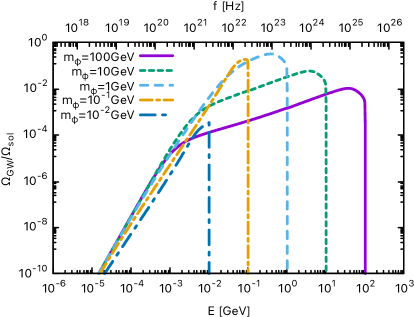
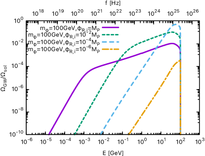
Figure 1: (Left) The present graviton spectrum from the boson star decay for $\phi_{R,i}=M_{\rm Pl}$ with $m=100,10,1,10^{-1},10^{-2}\,{\rm GeV}$. (Right) The spectrum for $m=100\,{\rm GeV}$ with $\phi_{R,i}=(1,10^{-2},10^{-4},10^{-6})\times M_{\rm Pl}$. We are assuming that the boson star is long-lived and the dominant part comes from the boson star decaying at the present universe.

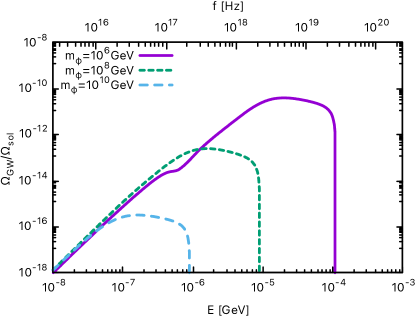
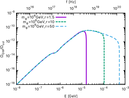
Figure 2: The present stochastic gravitational wave spectrum from the Q-ball decay. (Left) We have taken $m=10^{6},10^{8},10^{10}\,{\rm GeV}$ with $\varphi_{R,i}=M_{\rm Pl}$ and $\bar{\varphi}=0.1M_{\rm Pl}$, i.e., $r\equiv\varphi_{R,i}/\bar{\varphi}=10$. (Right) We have taken $m=10^{6}\,{\rm GeV}$ and $r=1.5,10,50$ with $\varphi_{R,i}=M_{\rm Pl}$ fixed. The graviton production stops in the early universe when the orbit of the complex scalar becomes circular and the cutoff frequency roughly corresponds to the gravitons produced at this epoch.

6 Discussion and conclusions

It is known that the cosmological dynamics of scalar or vector fields can lead to the formation of soliton-like objects such as an oscillon, Q-ball or boson stars. Oscillons/Q-balls are stabilized by self-interactions and boson stars are stabilized by gravitational interactions. They may have significant impacts on the early universe history, although still complete understandings of their dynamics have not been reached yet. One of the important properties of the soliton is its lifetime. There have been many studies for estimating the soliton lifetime, most of which focused on the emission of relativistic particles due to self-interactions.

In this paper we point out that there is a universal decay process of the solitons due to the gravitational interactions, i.e., quantum decay of a soliton into the graviton pair. This decay channel exists even for a free (scalar or vector) field with a minimal coupling to gravity and provides a strict upper limit on their lifetime. Although the solitons are spherically symmetric, its gravitational potential has an oscillating component in time, which leads to the production of gravitational waves (gravitons) via quantum decay process. The quantum decay rate into gravitons has a power-law dependence on the size of solitons, which should be compared with the exponentially-suppressed classical decay rate. Therefore, it can be the dominant channel for boson stars consisting of fuzzy dark matter or vector dark matter without a kinetic mixing. We have discussed the evolution of solitons via the quantum decay and calculated the spectrum of stochastic gravitational waves. Although the amplitude of gravitational waves is too small to be detected in the near future, the spectrum has an unique shape with a broken power law at a low frequency and a sharp cutoff at a high frequency.

References

- (1) R. D. Peccei and H. R. Quinn, CP Conservation in the Presence of Instantons, Phys. Rev. Lett. 38 (1977) 1440.
- (2) R. D. Peccei and H. R. Quinn, Constraints Imposed by CP Conservation in the Presence of Instantons, Phys. Rev. D 16 (1977) 1791.
- (3) J. Preskill, M. B. Wise and F. Wilczek, Cosmology of the Invisible Axion, Phys. Lett. B 120 (1983) 127.
- (4) L. F. Abbott and P. Sikivie, A Cosmological Bound on the Invisible Axion, Phys. Lett. B 120 (1983) 133.
- (5) M. Dine and W. Fischler, The Not So Harmless Axion, Phys. Lett. B 120 (1983) 137.
- (6) D. Antypas et al., New Horizons: Scalar and Vector Ultralight Dark Matter, 2203.14915.
- (7) A. E. Nelson and J. Scholtz, Dark Light, Dark Matter and the Misalignment Mechanism, Phys. Rev. D 84 (2011) 103501 [1105.2812].
- (8) P. Arias, D. Cadamuro, M. Goodsell, J. Jaeckel, J. Redondo and A. Ringwald, WISPy Cold Dark Matter, JCAP 06 (2012) 013 [1201.5902].
- (9) K. Nakayama, Vector Coherent Oscillation Dark Matter, JCAP 10 (2019) 019 [1907.06243].
- (10) K. Nakayama, Constraint on Vector Coherent Oscillation Dark Matter with Kinetic Function, JCAP 08 (2020) 033 [2004.10036].
- (11) N. Kitajima and K. Nakayama, Viable Vector Coherent Oscillation Dark Matter, 2303.04287.
- (12) A. J. Long and L.-T. Wang, Dark Photon Dark Matter from a Network of Cosmic Strings, Phys. Rev. D 99 (2019) 063529 [1901.03312].
- (13) N. Kitajima and K. Nakayama, Dark Photon Dark Matter from Cosmic Strings and Gravitational Wave Background, 2212.13573.
- (14) K. Nakayama and W. Yin, Hidden photon and axion dark matter from symmetry breaking, JHEP 10 (2021) 026 [2105.14549].
- (15) B. Salehian, M. A. Gorji, H. Firouzjahi and S. Mukohyama, Vector dark matter production from inflation with symmetry breaking, Phys. Rev. D 103 (2021) 063526 [2010.04491].
- (16) H. Firouzjahi, M. A. Gorji, S. Mukohyama and B. Salehian, Dark photon dark matter from charged inflaton, JHEP 06 (2021) 050 [2011.06324].
- (17) P. Agrawal, N. Kitajima, M. Reece, T. Sekiguchi and F. Takahashi, Relic Abundance of Dark Photon Dark Matter, Phys. Lett. B 801 (2020) 135136 [1810.07188].
- (18) J. A. Dror, K. Harigaya and V. Narayan, Parametric Resonance Production of Ultralight Vector Dark Matter, Phys. Rev. D 99 (2019) 035036 [1810.07195].
- (19) R. T. Co, A. Pierce, Z. Zhang and Y. Zhao, Dark Photon Dark Matter Produced by Axion Oscillations, Phys. Rev. D 99 (2019) 075002 [1810.07196].
- (20) M. Bastero-Gil, J. Santiago, L. Ubaldi and R. Vega-Morales, Vector dark matter production at the end of inflation, JCAP 04 (2019) 015 [1810.07208].
- (21) R. T. Co, K. Harigaya and A. Pierce, Gravitational waves and dark photon dark matter from axion rotations, JHEP 12 (2021) 099 [2104.02077].
- (22) N. Kitajima and F. Takahashi, Resonant production of dark photons from axion without a large coupling, 2303.05492.
- (23) P. W. Graham, J. Mardon and S. Rajendran, Vector Dark Matter from Inflationary Fluctuations, Phys. Rev. D 93 (2016) 103520 [1504.02102].
- (24) Y. Ema, K. Nakayama and Y. Tang, Production of purely gravitational dark matter: the case of fermion and vector boson, JHEP 07 (2019) 060 [1903.10973].
- (25) A. Ahmed, B. Grzadkowski and A. Socha, Gravitational production of vector dark matter, JHEP 08 (2020) 059 [2005.01766].
- (26) K. Nakayama and Y. Tang, Gravitational Production of Hidden Photon Dark Matter in Light of the XENON1T Excess, Phys. Lett. B 811 (2020) 135977 [2006.13159].
- (27) E. W. Kolb and A. J. Long, Completely dark photons from gravitational particle production during the inflationary era, JHEP 03 (2021) 283 [2009.03828].
- (28) A. Arvanitaki, S. Dimopoulos, M. Galanis, D. Racco, O. Simon and J. O. Thompson, Dark QED from inflation, JHEP 11 (2021) 106 [2108.04823].
- (29) T. Sato, F. Takahashi and M. Yamada, Gravitational production of dark photon dark matter with mass generated by the Higgs mechanism, JCAP 08 (2022) 022 [2204.11896].
- (30) A. H. Guth, M. P. Hertzberg and C. Prescod-Weinstein, Do Dark Matter Axions Form a Condensate with Long-Range Correlation?, Phys. Rev. D 92 (2015) 103513 [1412.5930].
- (31) D. J. Kaup, Klein-Gordon Geon, Phys. Rev. 172 (1968) 1331.
- (32) R. Ruffini and S. Bonazzola, Systems of selfgravitating particles in general relativity and the concept of an equation of state, Phys. Rev. 187 (1969) 1767.
- (33) M. Colpi, S. L. Shapiro and I. Wasserman, Boson Stars: Gravitational Equilibria of Selfinteracting Scalar Fields, Phys. Rev. Lett. 57 (1986) 2485.
- (34) E. Seidel and W. M. Suen, Oscillating soliton stars, Phys. Rev. Lett. 66 (1991) 1659.
- (35) I. I. Tkachev, On the possibility of Bose star formation, Phys. Lett. B 261 (1991) 289.
- (36) E. W. Kolb and I. I. Tkachev, Axion miniclusters and Bose stars, Phys. Rev. Lett. 71 (1993) 3051 [hep-ph/9303313].
- (37) E. W. Kolb and I. I. Tkachev, Nonlinear axion dynamics and formation of cosmological pseudosolitons, Phys. Rev. D 49 (1994) 5040 [astro-ph/9311037].
- (38) H.-Y. Schive, M.-H. Liao, T.-P. Woo, S.-K. Wong, T. Chiueh, T. Broadhurst et al., Understanding the Core-Halo Relation of Quantum Wave Dark Matter from 3D Simulations, Phys. Rev. Lett. 113 (2014) 261302 [1407.7762].
- (39) D. G. Levkov, A. G. Panin and I. I. Tkachev, Gravitational Bose-Einstein condensation in the kinetic regime, Phys. Rev. Lett. 121 (2018) 151301 [1804.05857].
- (40) J. Y. Widdicombe, T. Helfer, D. J. E. Marsh and E. A. Lim, Formation of Relativistic Axion Stars, JCAP 10 (2018) 005 [1806.09367].
- (41) B. Eggemeier and J. C. Niemeyer, Formation and mass growth of axion stars in axion miniclusters, Phys. Rev. D 100 (2019) 063528 [1906.01348].
- (42) J. Chen, X. Du, E. W. Lentz, D. J. E. Marsh and J. C. Niemeyer, New insights into the formation and growth of boson stars in dark matter halos, Phys. Rev. D 104 (2021) 083022 [2011.01333].
- (43) E. Braaten, A. Mohapatra and H. Zhang, Dense Axion Stars, Phys. Rev. Lett. 117 (2016) 121801 [1512.00108].
- (44) E. Braaten, A. Mohapatra and H. Zhang, Emission of Photons and Relativistic Axions from Axion Stars, Phys. Rev. D 96 (2017) 031901 [1609.05182].
- (45) L. Visinelli, S. Baum, J. Redondo, K. Freese and F. Wilczek, Dilute and dense axion stars, Phys. Lett. B 777 (2018) 64 [1710.08910].
- (46) E. D. Schiappacasse and M. P. Hertzberg, Analysis of Dark Matter Axion Clumps with Spherical Symmetry, JCAP 01 (2018) 037 [1710.04729].
- (47) J. Veltmaat, J. C. Niemeyer and B. Schwabe, Formation and structure of ultralight bosonic dark matter halos, Phys. Rev. D 98 (2018) 043509 [1804.09647].
- (48) P.-H. Chavanis, Mass-radius relation of Newtonian self-gravitating Bose-Einstein condensates with short-range interactions: I. Analytical results, Phys. Rev. D 84 (2011) 043531 [1103.2050].
- (49) P. H. Chavanis and L. Delfini, Mass-radius relation of Newtonian self-gravitating Bose-Einstein condensates with short-range interactions: II. Numerical results, Phys. Rev. D 84 (2011) 043532 [1103.2054].
- (50) J. Eby, K. Mukaida, M. Takimoto, L. C. R. Wijewardhana and M. Yamada, Classical nonrelativistic effective field theory and the role of gravitational interactions, Phys. Rev. D 99 (2019) 123503 [1807.09795].
- (51) K. Mukaida, M. Takimoto and M. Yamada, On Longevity of I-ball/Oscillon, JHEP 03 (2017) 122 [1612.07750].
- (52) J. H.-H. Chan, S. Sibiryakov and W. Xue, Condensation and Evaporation of Boson Stars, 2207.04057.
- (53) K. Fujikura, M. P. Hertzberg, E. D. Schiappacasse and M. Yamaguchi, Microlensing constraints on axion stars including finite lens and source size effects, Phys. Rev. D 104 (2021) 123012 [2109.04283].
- (54) D. Ellis, D. J. E. Marsh, B. Eggemeier, J. Niemeyer, J. Redondo and K. Dolag, Structure of axion miniclusters, Phys. Rev. D 106 (2022) 103514 [2204.13187].
- (55) I. L. Bogolyubsky and V. G. Makhankov, On the Pulsed Soliton Lifetime in Two Classical Relativistic Theory Models, JETP Lett. 24 (1976) 12.
- (56) H. Segur and M. D. Kruskal, Nonexistence of Small Amplitude Breather Solutions in Theory, Phys. Rev. Lett. 58 (1987) 747.
- (57) M. Gleiser, Pseudostable bubbles, Phys. Rev. D 49 (1994) 2978 [hep-ph/9308279].
- (58) E. J. Copeland, M. Gleiser and H. R. Muller, Oscillons: Resonant configurations during bubble collapse, Phys. Rev. D 52 (1995) 1920 [hep-ph/9503217].
- (59) M. Gleiser and A. Sornborger, Longlived localized field configurations in small lattices: Application to oscillons, Phys. Rev. E 62 (2000) 1368 [patt-sol/9909002].
- (60) E. P. Honda and M. W. Choptuik, Fine structure of oscillons in the spherically symmetric phi**4 Klein-Gordon model, Phys. Rev. D 65 (2002) 084037 [hep-ph/0110065].
- (61) S. Kasuya, M. Kawasaki and F. Takahashi, I-balls, Phys. Lett. B 559 (2003) 99 [hep-ph/0209358].
- (62) G. Fodor, P. Forgacs, P. Grandclement and I. Racz, Oscillons and Quasi-breathers in the phi**4 Klein-Gordon model, Phys. Rev. D 74 (2006) 124003 [hep-th/0609023].
- (63) G. Fodor, P. Forgacs, Z. Horvath and M. Mezei, Computation of the radiation amplitude of oscillons, Phys. Rev. D 79 (2009) 065002 [0812.1919].
- (64) M. Gleiser and D. Sicilia, Analytical Characterization of Oscillon Energy and Lifetime, Phys. Rev. Lett. 101 (2008) 011602 [0804.0791].
- (65) M. Gleiser and D. Sicilia, A General Theory of Oscillon Dynamics, Phys. Rev. D 80 (2009) 125037 [0910.5922].
- (66) M. A. Amin and D. Shirokoff, Flat-top oscillons in an expanding universe, Phys. Rev. D 81 (2010) 085045 [1002.3380].
- (67) M. A. Amin, R. Easther, H. Finkel, R. Flauger and M. P. Hertzberg, Oscillons After Inflation, Phys. Rev. Lett. 108 (2012) 241302 [1106.3335].
- (68) P. Salmi and M. Hindmarsh, Radiation and Relaxation of Oscillons, Phys. Rev. D 85 (2012) 085033 [1201.1934].
- (69) P. M. Saffin, P. Tognarelli and A. Tranberg, Oscillon Lifetime in the Presence of Quantum Fluctuations, JHEP 08 (2014) 125 [1401.6168].
- (70) K. Mukaida and M. Takimoto, Correspondence of I- and Q-balls as Non-relativistic Condensates, JCAP 08 (2014) 051 [1405.3233].
- (71) M. Kawasaki, F. Takahashi and N. Takeda, Adiabatic Invariance of Oscillons/I-balls, Phys. Rev. D 92 (2015) 105024 [1508.01028].
- (72) G. Fodor, P. Forgacs, Z. Horvath and A. Lukacs, Small amplitude quasi-breathers and oscillons, Phys. Rev. D 78 (2008) 025003 [0802.3525].
- (73) E. Braaten, A. Mohapatra and H. Zhang, Nonrelativistic Effective Field Theory for Axions, Phys. Rev. D 94 (2016) 076004 [1604.00669].
- (74) M. H. Namjoo, A. H. Guth and D. I. Kaiser, Relativistic Corrections to Nonrelativistic Effective Field Theories, Phys. Rev. D 98 (2018) 016011 [1712.00445].
- (75) E. Braaten, A. Mohapatra and H. Zhang, Classical Nonrelativistic Effective Field Theories for a Real Scalar Field, Phys. Rev. D 98 (2018) 096012 [1806.01898].
- (76) D. G. Levkov, V. E. Maslov, E. Y. Nugaev and A. G. Panin, An Effective Field Theory for large oscillons, JHEP 12 (2022) 079 [2208.04334].
- (77) A. Vaquero, J. Redondo and J. Stadler, Early seeds of axion miniclusters, JCAP 04 (2019) 012 [1809.09241].
- (78) A. Arvanitaki, S. Dimopoulos, M. Galanis, L. Lehner, J. O. Thompson and K. Van Tilburg, Large-misalignment mechanism for the formation of compact axion structures: Signatures from the QCD axion to fuzzy dark matter, Phys. Rev. D 101 (2020) 083014 [1909.11665].
- (79) E. J. Copeland, S. Pascoli and A. Rajantie, Dynamics of tachyonic preheating after hybrid inflation, Phys. Rev. D 65 (2002) 103517 [hep-ph/0202031].
- (80) K. Inomata, K. Kohri, T. Nakama and T. Terada, Enhancement of Gravitational Waves Induced by Scalar Perturbations due to a Sudden Transition from an Early Matter Era to the Radiation Era, Phys. Rev. D 100 (2019) 043532 [1904.12879].
- (81) K. D. Lozanov and V. Takhistov, Enhanced Gravitational Waves from Inflaton Oscillons, 2204.07152.
- (82) P. Adshead and K. D. Lozanov, Self-gravitating Vector Dark Matter, Phys. Rev. D 103 (2021) 103501 [2101.07265].
- (83) M. Jain and M. A. Amin, Polarized solitons in higher-spin wave dark matter, Phys. Rev. D 105 (2022) 056019 [2109.04892].
- (84) H.-Y. Zhang, M. Jain and M. A. Amin, Polarized vector oscillons, Phys. Rev. D 105 (2022) 096037 [2111.08700].
- (85) M. A. Amin, A. J. Long and E. D. Schiappacasse, Photons from dark photon solitons via parametric resonance, 2301.11470.
- (86) M. Gorghetto, E. Hardy, J. March-Russell, N. Song and S. M. West, Dark photon stars: formation and role as dark matter substructure, JCAP 08 (2022) 018 [2203.10100].
- (87) M. A. Amin, M. Jain, R. Karur and P. Mocz, Small-scale structure in vector dark matter, JCAP 08 (2022) 014 [2203.11935].
- (88) M. Jain, M. A. Amin, J. Thomas and W. Wanichwecharungruang, Kinetic relaxation and Bose-star formation in multicomponent dark matter- I, 2304.01985.
- (89) J. Eby, P. Suranyi and L. C. R. Wijewardhana, The Lifetime of Axion Stars, Mod. Phys. Lett. A 31 (2016) 1650090 [1512.01709].
- (90) J. Eby, M. Ma, P. Suranyi and L. C. R. Wijewardhana, Decay of Ultralight Axion Condensates, JHEP 01 (2018) 066 [1705.05385].
- (91) M. Ibe, M. Kawasaki, W. Nakano and E. Sonomoto, Decay of I-ball/Oscillon in Classical Field Theory, JHEP 04 (2019) 030 [1901.06130].
- (92) M. Ibe, M. Kawasaki, W. Nakano and E. Sonomoto, Fragileness of Exact I-ball/Oscillon, Phys. Rev. D 100 (2019) 125021 [1908.11103].
- (93) H.-Y. Zhang, M. A. Amin, E. J. Copeland, P. M. Saffin and K. D. Lozanov, Classical Decay Rates of Oscillons, JCAP 07 (2020) 055 [2004.01202].
- (94) H.-Y. Zhang, Gravitational effects on oscillon lifetimes, JCAP 03 (2021) 102 [2011.11720].
- (95) P. Grandclement, G. Fodor and P. Forgacs, Numerical simulation of oscillatons: extracting the radiating tail, Phys. Rev. D 84 (2011) 065037 [1107.2791].
- (96) G. Fodor, P. Forgacs and M. Mezei, Mass loss and longevity of gravitationally bound oscillating scalar lumps (oscillatons) in D-dimensions, Phys. Rev. D 81 (2010) 064029 [0912.5351].
- (97) D. N. Page, Classical and quantum decay of oscillatons: Oscillating selfgravitating real scalar field solitons, Phys. Rev. D 70 (2004) 023002 [gr-qc/0310006].
- (98) J. Eby, L. Street, P. Suranyi and L. C. R. Wijewardhana, Global view of axion stars with nearly Planck-scale decay constants, Phys. Rev. D 103 (2021) 063043 [2011.09087].
- (99) M. P. Hertzberg, Quantum Radiation of Oscillons, Phys. Rev. D 82 (2010) 045022 [1003.3459].
- (100) M. Kawasaki and M. Yamada, Decay rates of Gaussian-type I-balls and Bose-enhancement effects in 3+1 dimensions, JCAP 02 (2014) 001 [1311.0985].
- (101) M. P. Hertzberg and E. D. Schiappacasse, Dark Matter Axion Clump Resonance of Photons, JCAP 11 (2018) 004 [1805.00430].
- (102) Y. Ema, R. Jinno, K. Mukaida and K. Nakayama, Gravitational Effects on Inflaton Decay, JCAP 05 (2015) 038 [1502.02475].
- (103) Y. Ema, R. Jinno, K. Mukaida and K. Nakayama, Gravitational particle production in oscillating backgrounds and its cosmological implications, Phys. Rev. D 94 (2016) 063517 [1604.08898].
- (104) Y. Tang and Y.-L. Wu, On Thermal Gravitational Contribution to Particle Production and Dark Matter, Phys. Lett. B 774 (2017) 676 [1708.05138].
- (105) Y. Ema, K. Nakayama and Y. Tang, Production of Purely Gravitational Dark Matter, JHEP 09 (2018) 135 [1804.07471].
- (106) D. J. H. Chung, E. W. Kolb and A. J. Long, Gravitational production of super-Hubble-mass particles: an analytic approach, JHEP 01 (2019) 189 [1812.00211].
- (107) Y. Mambrini and K. A. Olive, Gravitational Production of Dark Matter during Reheating, Phys. Rev. D 103 (2021) 115009 [2102.06214].
- (108) E. E. Basso and D. J. H. Chung, Computation of gravitational particle production using adiabatic invariants, JHEP 11 (2021) 146 [2108.01653].
- (109) S. Clery, Y. Mambrini, K. A. Olive and S. Verner, Gravitational portals in the early Universe, Phys. Rev. D 105 (2022) 075005 [2112.15214].
- (110) M. R. Haque and D. Maity, Gravitational dark matter: Free streaming and phase space distribution, Phys. Rev. D 106 (2022) 023506 [2112.14668].
- (111) E. D. Schiappacasse and L. H. Ford, Graviton Creation by Small Scale Factor Oscillations in an Expanding Universe, Phys. Rev. D 94 (2016) 084030 [1602.08416].
- (112) Y. Ema, R. Jinno and K. Nakayama, High-frequency Graviton from Inflaton Oscillation, JCAP 09 (2020) 015 [2006.09972].
- (113) M. Garny, M. Sandora and M. S. Sloth, Planckian Interacting Massive Particles as Dark Matter, Phys. Rev. Lett. 116 (2016) 101302 [1511.03278].
- (114) Y. Tang and Y.-L. Wu, Pure Gravitational Dark Matter, Its Mass and Signatures, Phys. Lett. B 758 (2016) 402 [1604.04701].
- (115) M. Garny, A. Palessandro, M. Sandora and M. S. Sloth, Theory and Phenomenology of Planckian Interacting Massive Particles as Dark Matter, JCAP 02 (2018) 027 [1709.09688].
- (116) C. Gross, S. Karamitsos, G. Landini and A. Strumia, Gravitational Vector Dark Matter, JHEP 03 (2021) 174 [2012.12087].
- (117) L. H. Ford, Gravitational Particle Creation and Inflation, Phys. Rev. D 35 (1987) 2955.
- (118) D. J. H. Chung, P. Crotty, E. W. Kolb and A. Riotto, On the Gravitational Production of Superheavy Dark Matter, Phys. Rev. D 64 (2001) 043503 [hep-ph/0104100].
- (119) D. J. H. Chung, L. L. Everett, H. Yoo and P. Zhou, Gravitational Fermion Production in Inflationary Cosmology, Phys. Lett. B 712 (2012) 147 [1109.2524].
- (120) S. Hashiba and J. Yokoyama, Gravitational particle creation for dark matter and reheating, Phys. Rev. D 99 (2019) 043008 [1812.10032].
- (121) S. R. Coleman, Q-balls, Nucl. Phys. B 262 (1985) 263.
- (122) R. Friedberg, T. D. Lee and Y. Pang, MINI - SOLITON STARS, Phys. Rev. D 35 (1987) 3640.
- (123) A. G. Cohen, S. R. Coleman, H. Georgi and A. Manohar, The Evaporation of Balls, Nucl. Phys. B 272 (1986) 301.
- (124) A. Kusenko, Small Q balls, Phys. Lett. B 404 (1997) 285 [hep-th/9704073].
- (125) A. Kusenko, Solitons in the supersymmetric extensions of the standard model, Phys. Lett. B 405 (1997) 108 [hep-ph/9704273].
- (126) A. Kusenko and M. E. Shaposhnikov, Supersymmetric Q balls as dark matter, Phys. Lett. B 418 (1998) 46 [hep-ph/9709492].
- (127) I. Affleck and M. Dine, A New Mechanism for Baryogenesis, Nucl. Phys. B 249 (1985) 361.
- (128) M. Dine, L. Randall and S. D. Thomas, Baryogenesis from flat directions of the supersymmetric standard model, Nucl. Phys. B 458 (1996) 291 [hep-ph/9507453].
- (129) A. D. Dolgov and D. P. Kirilova, ON PARTICLE CREATION BY A TIME DEPENDENT SCALAR FIELD, Sov. J. Nucl. Phys. 51 (1990) 172.
- (130) J. H. Traschen and R. H. Brandenberger, Particle Production During Out-of-equilibrium Phase Transitions, Phys. Rev. D 42 (1990) 2491.
- (131) Y. Shtanov, J. H. Traschen and R. H. Brandenberger, Universe reheating after inflation, Phys. Rev. D 51 (1995) 5438 [hep-ph/9407247].
- (132) L. Kofman, A. D. Linde and A. A. Starobinsky, Towards the theory of reheating after inflation, Phys. Rev. D 56 (1997) 3258 [hep-ph/9704452].
- (133) M. Kawasaki, K. Konya and F. Takahashi, Q-ball instability due to U(1) breaking, Phys. Lett. B 619 (2005) 233 [hep-ph/0504105].
- (134) T. Hiramatsu, M. Kawasaki and F. Takahashi, Numerical study of Q-ball formation in gravity mediation, JCAP 06 (2010) 008 [1003.1779].
- (135) F. Hasegawa, J.-P. Hong and M. Suzuki, More about Q-ball with elliptical orbit, Phys. Lett. B 798 (2019) 135001 [1903.07281].
- (136) R. T. Co and K. Harigaya, Axiogenesis, Phys. Rev. Lett. 124 (2020) 111602 [1910.02080].
- (137) R. T. Co, L. J. Hall and K. Harigaya, Axion Kinetic Misalignment Mechanism, Phys. Rev. Lett. 124 (2020) 251802 [1910.14152].
- (138) S.-Y. Zhou, E. J. Copeland, R. Easther, H. Finkel, Z.-G. Mou and P. M. Saffin, Gravitational Waves from Oscillon Preheating, JHEP 10 (2013) 026 [1304.6094].
- (139) S. Antusch, F. Cefala and S. Orani, Gravitational waves from oscillons after inflation, Phys. Rev. Lett. 118 (2017) 011303 [1607.01314].
- (140) J. Liu, Z.-K. Guo, R.-G. Cai and G. Shiu, Gravitational Waves from Oscillons with Cuspy Potentials, Phys. Rev. Lett. 120 (2018) 031301 [1707.09841].
- (141) K. D. Lozanov and M. A. Amin, Self-resonance after inflation: oscillons, transients and radiation domination, Phys. Rev. D 97 (2018) 023533 [1710.06851].
- (142) M. A. Amin, J. Braden, E. J. Copeland, J. T. Giblin, C. Solorio, Z. J. Weiner et al., Gravitational waves from asymmetric oscillon dynamics?, Phys. Rev. D 98 (2018) 024040 [1803.08047].
- (143) N. Kitajima, J. Soda and Y. Urakawa, Gravitational wave forest from string axiverse, JCAP 10 (2018) 008 [1807.07037].
- (144) J. Liu, Z.-K. Guo, R.-G. Cai and G. Shiu, Gravitational wave production after inflation with cuspy potentials, Phys. Rev. D 99 (2019) 103506 [1812.09235].
- (145) K. D. Lozanov and M. A. Amin, Gravitational perturbations from oscillons and transients after inflation, Phys. Rev. D 99 (2019) 123504 [1902.06736].
- (146) T. Hiramatsu, E. I. Sfakianakis and M. Yamaguchi, Gravitational wave spectra from oscillon formation after inflation, JHEP 03 (2021) 021 [2011.12201].
- (147) X.-X. Kou, J. B. Mertens, C. Tian and S.-Y. Zhou, Gravitational waves from fully general relativistic oscillon preheating, Phys. Rev. D 105 (2022) 123505 [2112.07626].
- (148) M. A. G. Garcia and M. Pierre, Reheating after Inflaton Fragmentation, 2306.08038.
- (149) A. Kusenko and A. Mazumdar, Gravitational waves from fragmentation of a primordial scalar condensate into Q-balls, Phys. Rev. Lett. 101 (2008) 211301 [0807.4554].
- (150) A. Kusenko, A. Mazumdar and T. Multamaki, Gravitational waves from the fragmentation of a supersymmetric condensate, Phys. Rev. D 79 (2009) 124034 [0902.2197].
- (151) T. Chiba, K. Kamada and M. Yamaguchi, Gravitational Waves from Q-ball Formation, Phys. Rev. D 81 (2010) 083503 [0912.3585].
- (152) Y. Ema, K. Mukaida and K. Nakayama, Scalar field couplings to quadratic curvature and decay into gravitons, JHEP 05 (2022) 087 [2112.12774].
- (153) A. Ejlli, D. Ejlli, A. M. Cruise, G. Pisano and H. Grote, Upper limits on the amplitude of ultra-high-frequency gravitational waves from graviton to photon conversion, Eur. Phys. J. C 79 (2019) 1032 [1908.00232].
- (154) A. Ringwald, J. Schutte-Engel and C. Tamarit, Gravitational Waves as a Big Bang Thermometer, JCAP 03 (2021) 054 [2011.04731].
- (155) N. Aggarwal et al., Challenges and opportunities of gravitational-wave searches at MHz to GHz frequencies, Living Rev. Rel. 24 (2021) 4 [2011.12414].
- (156) A. Berlin, D. Blas, R. Tito D’Agnolo, S. A. R. Ellis, R. Harnik, Y. Kahn et al., Detecting high-frequency gravitational waves with microwave cavities, Phys. Rev. D 105 (2022) 116011 [2112.11465].
- (157) V. Domcke, C. Garcia-Cely and N. L. Rodd, Novel Search for High-Frequency Gravitational Waves with Low-Mass Axion Haloscopes, Phys. Rev. Lett. 129 (2022) 041101 [2202.00695].
- (158) M. E. Tobar, C. A. Thomson, W. M. Campbell, A. Quiskamp, J. F. Bourhill, B. T. McAllister et al., Comparing Instrument Spectral Sensitivity of Dissimilar Electromagnetic Haloscopes to Axion Dark Matter and High Frequency Gravitational Waves, Symmetry 14 (2022) 2165 [2209.03004].
- (159) A. D. Dolgov and D. Ejlli, Conversion of relic gravitational waves into photons in cosmological magnetic fields, JCAP 12 (2012) 003 [1211.0500].
- (160) V. Domcke and C. Garcia-Cely, Potential of radio telescopes as high-frequency gravitational wave detectors, Phys. Rev. Lett. 126 (2021) 021104 [2006.01161].
- (161) S. Ramazanov, R. Samanta, G. Trenkler and F. R. Urban, Shimmering gravitons in the gamma-ray sky, 2304.11222.
- (162) T. Liu, J. Ren and C. Zhang, Detecting High-Frequency Gravitational Waves in Planetary Magnetosphere, 2305.01832.
- (163) A. Ito, K. Kohri and K. Nakayama, Probing high frequency gravitational waves with pulsars, 2305.13984.