Disentangle Neutrino Electromagnetic Properties with Atomic Radiative Pair Emission

Abstract

We elaborate the possibility of using the atomic radiative emission of neutrino pair (RENP) to probe the neutrino electromagnetic properties, including magnetic and electric dipole moments, charge radius, and anapole. With the typical $\mathcal{O}$(eV) momentum transfer, the atomic RENP is sensitive to not just the tiny neutrino masses but also very light mediators to which the massless photon belongs. The neutrino EM properties introduce extra contribution besides the SM one induced by the heavy $W/Z$ gauge bosons. Since the associated photon spectrum is divided into several sections whose boundaries are determined by the final-state neutrino masses, it is possible to identify the individual neutrino EM form factor elements. Most importantly, scanning the photon spectrum inside the particular section with deviation from the SM prediction once observed allows identification of the neutrino EM form factor type. The RENP provides an ultimate way of disentangling the neutrino EM properties to go beyond the current experimental searches or observations.

1 Introduction

The existence of neutrinos is indicated by the continuous beta decay spectrum and informally proposed by Pauli in his famous letter to the participants of the Tübingen conference on radioactivity on December 4, 1930 [1]. In exactly the same letter, Pauli suggested that “the neutrino at rest is a magnetic dipole with a certain moment” as the possible interaction that neutrino may have. So, the neutrino EM properties are actually the very first studied. While Pauli only mentioned magnetic moment, the general neutrino ($\nu$) coupling to photons ($A$) contain four independent form factor types at the vanishing momentum transfer limit ($q^{2}\rightarrow 0)$ [2, 3],

$$H_{EM}=\overline{\nu}\left[-i\sigma_{\mu\nu}q^{\nu}\left(\mu_{\nu}+i\epsilon_{\nu}\gamma_{5}\right)+\left(\gamma_{\mu}-\frac{q_{\mu}\not{q}}{q^{2}}\right)q^{2}\left(\frac{\langle r^{2}_{\nu}\rangle}{6}+a_{\nu}\gamma_{5}\right)\right]\nu A^{\mu}(q),$$ (1.1)

where $\mu_{\nu}$, $\epsilon_{\nu}$, $\langle r^{2}_{\nu}\rangle$, and $a_{\nu}$ are the neutrino magnetic dipole moment (MDM), electric dipole moment (EDM), charge radius, and anapole, respectively. Within the three-neutrino paradigm, all the neutrino EM properties are Hermitian matrices. In the Standard Model (SM) of particle physics, the tree-level coupling between neutrino and photon is zero [4] while the loop-induced electromagnetic couplings are highly suppressed. While the neutrino charge radius and anapole are suppressed by the Fermi constant [5, 6], the neutrino magnetic moment and electric dipole are further suppressed by the neutrino mass [7, 8, 9, 5].

Since the SM values for the neutrino EM properties are small, their observation is a window to possible new physics beyond the Standard Model (BSM) [10, 11, 12]. There are various ways of probing the neutrino EM properties. The neutrino scattering experiments measure the electron/nucleus recoil spectrum with existing constraints ranging from $10^{-7}\mu_{B}$ ($10^{-29}$ cm²) to $10^{-11}\mu_{B}$ ($10^{-32}$ cm²) for neutrino magnetic/electric moments (charge radius/anapole). Different neutrino sources have characteristic energy scales, such as accelerators ($0.2\,{\rm GeV}<E_{\nu}<20$ GeV) [13, 14, 15], reactors [16] ($1\,{\rm MeV}<E_{\nu}<50$ MeV), and the Sun (Super-K and Borexino with $0.4\,{\rm MeV}<E_{\nu}<20$ MeV which is larger than the one $2\,{\rm keV}<E_{\nu}<400$ keV at DM experiments) [17, 18, 19, 20, 21]. The neutrino decay observations can also put constraints by searching the decay photons in reactors [22] or distortions to the CMB spectrum [23], reaching $10^{-5}\mu_{B}$ to $10^{-8}\mu_{B}$. In addition, the stellar cooling due to plasmon decay ($\gamma^{*}\rightarrow\nu\bar{\nu}$) constraints the magnetic/electric moment (charge radius/anapole) to $\mathcal{O}(10^{-12}\,\mu_{B})$ ($\mathcal{O}(10^{-32})$ cm²) [24, 25, 26].

However, all existing searches presented above have intrinsic caveats. With neutrinos not being detected and especially difficult to disentangle their mass eigenstates, constraints are obtained as a combination of parameters involving both the neutrino mixing and form factor matrix elements [27] to introduce various degeneracies [28]. A single or just a handful of observations cannot disentangle and identify individual form factor elements. One possible solution [29] is the radiative emission of neutrino pair (RENP) from excited atoms [30, 31, 32, 33, 34, 35]. Since atomic transition energies are typically $\mathcal{O}({\rm eV})$, close to the neutrino mass values, RENP is an ideal place to test the light mediators that couples with neutrino and electrons [36], including the massless photon.

In this work we further show that RENP can disentangle all the neutrino EM properties ($\mu_{\nu}$, $\epsilon_{\nu}$, $\langle r^{2}_{\nu}\rangle$, and $a_{\nu}$) with details. In Sec. 2, we describe the general electromagnetic vertex properties to establish the formalism of neutrino EM form factors and summarize the existing experimental/observational constraints. The selection rules and details of how neutrino EM properties affect the RENP photon spectrum are presented in Sec. 3. Based on the theoretical formulas, we illustrate a practical strategy of scanning the photon spectrum to identify each form factor elements and their type in Sec. 4. Our discussions and conclusion can be found in Sec. 5.

2 Neutrino Eletromagnetic Properties

2.1 Electromagnetic Form Factors

The neutrino EM interaction is characterized as the neutrino current ($j_{\mu}^{(\nu)}$) in terms of a vertex function ($\Lambda_{\mu}^{ij}(q)$),

$$j_{\mu}^{(\nu)}\equiv\bar{u}(p_{i})\Lambda_{\mu}^{ij}(q)u(p_{j}),$$ (2.1)

with the momentum transfer $q\equiv p_{i}-p_{j}$ as difference between the initial ($p_{i}$) and final ($p_{j}$) neutrino momenta. Since the neutrino current vertex $\Lambda_{\mu}^{ij}(q)$ is a function of the momentum transfer $q$, it can be expanded as a linear combination of $q_{\mu}$, $\gamma_{\mu}$ and $\sigma_{\mu\nu}q^{\nu}$ to match the current Lorentz structure. Each type can be associated with a $\gamma_{5}$ to double the form factors $F_{A}^{ij}(q^{2})$ with $A=1,\dots,6$, [37],

$$\Lambda_{\mu}^{ij}\equiv q_{\mu}(F_{1}^{ij}+F_{2}^{ij}\gamma_{5})+\gamma_{\mu}(F_{3}^{ij}+F_{4}^{ij}\gamma_{5})+i\sigma_{\mu\nu}q^{\nu}(F^{ij}_{5}+F^{ij}_{6}i\gamma_{5}).$$ (2.2)

Then the coupling with a massless photon takes the form as $\mathcal{L}\ni A^{\mu}j^{(\nu)}_{\mu}$.

Note that the quantum electrodynamics (QED) gauge symmetry $U(1)_{\rm em}$ is not broken even in the presence of neutrino EM interactions. Consequently, the $U(1)_{\rm em}$ gauge invariance implies the conservation of the neutrino current, $q^{\mu}j_{\mu}^{(\nu)}=0$, which restricts two of the 6 form factors. Of the 6 form factors, the first two $F^{ij}_{1}=-F^{ij}_{3}(m_{i}-m_{j})/q^{2}$ and $F^{ij}_{2}=-F^{ij}_{4}(m_{i}+m_{j})q^{2}$ are expressed in terms of $F^{ij}_{3}$ and $F^{ij}_{4}$. It is interesting to observe that $F^{ij}_{1}$ is nonzero only for $m_{i}\neq m_{j}$. In other words, $F^{ij}_{1}$ has only off-diagonal elements. For the diagonal case, only $F^{ij}_{3}$ survives and the current conservation holds with vanishing $\bar{u}_{i}\not{q}u_{j}=(m_{i}-m_{j})\bar{u}_{i}u_{j}$ and $i=j$. Note that the current conservation does not require on-shell photon but on-shell fermions. Then Eq. (2.2) reduces to,

$$\Lambda_{\mu}^{ij}(q)\equiv\left(\gamma_{\mu}-\frac{q_{\mu}\not{q}}{q^{2}}\right)\left[f_{Q}^{ij}(q^{2})+f_{A}^{ij}(q^{2})q^{2}\gamma_{5}\right]-f_{M}^{ij}(q^{2})i\sigma_{\mu\nu}q^{\nu}+f_{E}^{ij}(q^{2})\sigma_{\mu\nu}q^{\nu}\gamma_{5}\,.$$ (2.3)

To make the physics picture more transparent, we have redefined, $f^{ij}_{Q}\equiv F^{ij}_{3}$ (electric charge), $f^{ij}_{A}\equiv F^{ij}_{4}/q^{2}$ (anapole), $f^{ij}_{M}\equiv-F^{ij}_{5}$ (magnetic dipole), and $f^{ij}_{E}\equiv F^{ij}_{6}$ (electric dipole), respectively. The hermiticity of the interaction Lagrangian further requires that $(f_{B}^{ij})^{\dagger}=f_{B}^{ij}$.

The form factors at $q^{2}\rightarrow 0$ give the values of the magnetic moment $\mu_{\nu}^{ij}\equiv f^{ij}_{M}(0)$, electric dipole $\epsilon_{\nu}^{ij}\equiv f^{ij}_{E}(0)$, charge $q_{\nu}^{ij}\equiv f^{ij}_{Q}(0)$, and anapole $a_{\nu}^{ij}\equiv f^{ij}_{A}(0)$. In the zero momentum transfer limit, these form factors have vanishing effect with the only exception of the electric charge while the other three are suppressed by either $q^{2}$ or $q^{\nu}$. Consequently, the neutrino charge is highly constrained, $|q_{\nu}|<3\times 10^{-21}e$ [22] and the next order expansion of $f^{ij}_{Q}$ provides the charge radius, $\langle r^{2}_{\nu}\rangle\equiv 6\left.df^{ij}_{Q}/dq^{2}\right|_{q^{2}=0}$.

For Majorana neutrinos, the current in Eq. (2.1) contains an extra term. While Dirac neutrino fields are formed with two sets of operators $a$ and $b$, $\nu^{(D)}\sim au+b^{\dagger}v$, the Majorana case has only one $a$, $\nu_{k}^{(M)}\sim au+a^{\dagger}v$. A general Majorana interaction $\mathcal{L}=\frac{1}{2}\bar{\nu}_{i}\Lambda_{\mu}^{ij}A^{\mu}\nu_{j}$ generates two contributions to the neutrino current,

$$j_{\mu}^{(\nu)}=\frac{1}{2}\left[\bar{u}(p_{i})\Lambda_{\mu}^{ij}(q)u(p_{j})-\bar{v}(p_{j})\Lambda_{\mu}^{ji}(q)v(p_{i})\right],$$ (2.4)

with switched indices $i$ and $j$. The charge conjugation transformation matrix $C$ in the spinors, $\overline{u}=v^{T}C^{-1}$, is used to swap $p_{i}\leftrightarrow p_{j}$ in the above equation to,

$$j_{\mu}^{(\nu)}=\bar{u}(p_{i})\left[\frac{\Lambda_{\mu}^{ij}(q)+C(\Lambda_{\mu}^{ij}(q))^{T}C^{-1}}{2}\right]u(p_{j})\,.$$ (2.5)

Since the charge conjugate transformation of the Lorentz structures follows,

$$C\Gamma^{T}C^{-1}=-\Gamma\,\quad{\rm for}\quad\Gamma=\gamma_{\mu},\sigma_{\mu\nu},\sigma_{\mu\nu}\gamma_{5}\,,\quad{\rm and}\quad C(\gamma_{\mu}\gamma_{5})^{T}C^{-1}=\gamma_{\mu}\gamma_{5}\,,$$ (2.6)

the extra contribution for Majorana neutrinos does not mix Lorentz structures and introduces at most a minus sign.

The only difference between Dirac/Majorana neutrinos with EM interactions is the form factor matrix pattern,

$$(q_{\nu}^{ij})^{T}=-q_{\nu}^{ij}\,,\quad(\mu_{\nu}^{ij})^{T}=-\mu_{\nu}^{ij}\,,\quad(\epsilon_{\nu}^{ij})^{T}=-\epsilon_{\nu}^{ij}\,,\quad{\rm and}\quad(a_{\nu}^{ij})^{T}=a_{\nu}^{ij}\,.$$ (2.7)

In other words, some form factors are forbidden for Majorana neutrinos and consequently the number of independent parameters is significantly reduced. Observing nonzero diagonal element $q^{ii}_{\nu}$, $\mu^{ii}_{\nu}$, or $\epsilon^{ii}_{\nu}$ is a direct evidence of the Dirac nature of neutrinos. In addition, the existence of electric dipole moment $\epsilon^{ij}_{\nu}$ indicates possible CP violation. For comparison, anapole violates both parity and charge conjugations, but preserves CP [37].

2.2 Existing Terrestrial and Celestial Tests

The constraints on the neutrino EM form factors are obtained from a variety of terrestrial experiments and astrophysical observations [37, 38]. Nevertheless, these existing measurements can only constrain combinations of the relevant form factor elements. In other words, there is no way to distinguish and identify the individual ones.

2.2.1 Terrestrial Tests with Electron Scattering

The terrestrial experiments typically use neutrino scattering with electron or nuclei via a $t$-channel photon exchange to probe the neutrino EM form factors. Either reactor, accelerator, or solar neutrinos are possible sources for such experiments. Currently, the strongest constraint comes from the neutrino scattering with electron. Such process can already be induced by the SM weak interactions with differential cross section [39, 40],

$$\left(\frac{d\sigma_{\nu_{i}e\rightarrow\nu_{j}e}}{dT_{r}}\right)_{\rm SM}=\frac{G_{F}^{2}m_{e}}{2\pi}\Biggl{\{}|v_{ji}\mp a_{ji}|^{2}+|v_{ji}\pm a_{ji}|^{2}\left(1-\frac{T_{r}}{E_{\nu_{i}}}\right)^{2}-\left(\left|v_{ji}\right|^{2}-|a_{ji}|^{2}\right)\frac{m_{e}T_{r}}{4E_{\nu_{i}}^{2}}\Biggr{\}},$$ (2.8)

where the upper (lower) sign is for the (anti-)neutrino scattering. The SM neutrino and electron EW interactions have been summarized into the axial and vector current couplings $a_{ij}\equiv-U_{ei}^{*}U_{ej}+\delta_{ij}/2$ and $v_{ij}\equiv-a_{ij}+2\sin\theta_{w}\delta_{ij}$ of the effective four-fermion operators, $\bar{e}\gamma_{\mu}(v_{ij}+a_{ij}\gamma_{5})e\times\bar{\nu}_{i}\gamma^{\mu}(1-\gamma_{5})\nu_{j}$. Both the charged and neutral currents mediated by the $W^{\pm}$ and $Z$ gauge bosons can contribute. The neutrino mixing matrix elements $U^{*}_{ei}$ and $U_{ej}$ arise from the charged current contribution with the flavor index $e$ for the involved electron in the initial and final states. Also, the neutrino external states are in their physical mass eigenstates. In other words, Eq. (2.8) considers the incoming neutrinos as incoherent states. The more general case with coherence, especially for neutrino oscillation experiments, is elaborated below.

Non-zero neutrino charge radius [41] and anapole [42] modify the effective vector current coupling $v_{ji}\rightarrow\widetilde{v}_{ji}$ as,

$$\widetilde{v}_{ij}\equiv v_{ij}+4\left[\frac{\langle r^{2}_{\nu}\rangle_{ij}}{6}-(a_{\nu})_{ij}\right]\frac{M_{W}^{2}\sin^{2}\theta_{w}}{e}.$$ (2.9)

Although the charge randius and anapole are associated with the neutrino vector and axial currents, respectively, their contributions can altogether combine into $v_{ij}$ but not $a_{ij}$. Note that $v_{ij}$ and $a_{ij}$ are actually associated with the electron bilinears in the effective four-fermion operators, not the neutrino ones.

Since both charge radius and anapole appear in the same place of $\widetilde{v}_{ij}$, an unfortunate degeneracy between them exists. Making it worse, the incoming neutrinos are typically coherent linear combination of mass eigenstates and oscillate over distance while the final-states neutrinos should be treated as the physical mass eigenstates. Being illusive, all the final-state neutrinos $\nu_{j}$ contribute to the electron scattering event rate as an inclusive cross section. The actual observable is a summation over the indices $i$ and $j$ in Eq. (2.8) with coefficients given by the neutrino mixing matrix elements [27]. In addition, the tiny neutrino masses are negligible and different final-state neutrinos have no actual difference. These lead to an accidental coincidence that the final-state neutrinos can also be taken as flavor states. For short baseline, no oscillation occurs and the couplings are written in the flavor basis, $\widetilde{v}_{\alpha\beta}\equiv\sum_{ij}U_{\alpha i}U_{\beta j}^{*}\widetilde{v}_{ij}$. Since $a_{\alpha\beta}=-\delta_{e\alpha}\delta_{e\beta}+\delta_{\alpha\beta}/2$ and $v_{\alpha\beta}=-a_{\alpha\beta}+2\sin\theta_{w}\delta_{\alpha\beta}$ are diagonal, the differential cross section in Eq. (2.8) becomes,

$$\frac{d\sigma_{\nu_{\alpha}e\rightarrow Xe}}{dT_{r}} =\frac{G_{F}^{2}m_{e}}{2\pi}\Biggl{\{}|\widetilde{v}_{\alpha\alpha}\mp a_{\alpha\alpha}|^{2}+|\widetilde{v}_{\alpha\alpha}\pm a_{\alpha\alpha}|^{2}\left(1-\frac{T_{r}}{E_{\nu}}\right)^{2}-\left(|\widetilde{v}_{\alpha\alpha}|^{2}-|a_{\alpha\alpha}|^{2}\right)\frac{m_{e}T_{r}}{4E_{\nu}^{2}}\Biggr{\}}$$

$$+\frac{\alpha m_{e}}{144}\sum_{\beta\neq\alpha}|\langle r^{2}_{\nu}\rangle_{\alpha\beta}^{\rm eff}|^{2}\left[1+\left(1-\frac{T_{r}}{E_{\nu}}\right)^{2}-\frac{m_{e}T_{r}}{4E_{\nu}^{2}}\right]\,.$$ (2.10)

Note that the diagonal elements $\langle r^{2}_{\nu}\rangle_{\alpha\alpha}$ and $(a_{\nu})_{\alpha\alpha}$ appear in the first line while the off-diagonal ones in the second line. Although the diagonal elements have interference with the SM contribution, the off-diagonal ones are standalone as square term in the second line.

For convenience, we have defined the effective charge radius as,

$$\langle r^{2}\rangle_{\alpha\beta}^{\rm eff}\equiv\sum_{ij}U_{\alpha i}U_{\beta j}^{*}\left[\langle r_{\nu}^{2}\rangle_{ij}-6(a_{\nu})_{ij}\right]\,.$$ (2.11)

With degeneracy among the charge radius, anapole, and the neutrino mixing matrix elements $U_{\alpha i}U^{*}_{\beta j}$, it is very hard to disentangle and identify the individual neutrino EM form factors.

A similar situation occurs for the magnetic ($\mu_{\nu}$) and electric dipole ($\epsilon_{\nu}$) moments. The cross-section in Eq. (2.8) receives corrections as [43],

$$\left(\frac{d\sigma_{\nu_{\alpha}e\rightarrow Xe}}{dT_{r}}\right)_{\mu,\epsilon}=\frac{\pi\alpha^{2}}{m_{e}^{2}}\left(\frac{1}{T_{r}}-\frac{1}{E_{\nu_{\alpha}}}\right)|\mu^{\rm eff}_{\alpha}|^{2},$$ (2.12)

with $X$ denoting any possible neutrino flavor or mass eigenstates. The effective magnetic moment $|\mu^{\rm eff}_{\alpha}|^{2}$ is defined as combination of the magnetic ($\mu_{\nu}$) and electric dipole ($\epsilon_{\nu}$) moments,

$$|\mu^{\rm eff}_{\alpha}|^{2} \equiv\sum_{ij}\left\{U_{\alpha i}(\mu^{2}_{\nu}+\epsilon^{2}_{\nu})_{ij}U_{\alpha j}^{*}+2\,{\rm Im}[U_{\alpha i}(\mu_{\nu}\epsilon_{\nu})_{ij}U_{\alpha j}^{*}]\right\}.$$ (2.13)

When defining the effective MDM $\mu^{\rm eff}_{\alpha}$, we have used the property that $\mu^{\dagger}_{\nu}=\mu_{\nu}$ and $\epsilon^{\dagger}_{\nu}=\epsilon_{\nu}$ are hermitian. Since $(\mu_{\nu})_{ij}$ and $(\epsilon_{\nu})_{ij}$ appear in similar ways, the neutrino scattering process cannot distinguish them. Multiple degeneracies exist not just for the charge radius and anapole, but also EDM and MDM. Although there are four form factors each with 6 elements, only few independent combinations can be measured.

The bound on the effective charge radius is obtained for only the diagonal elements, assuming vanishing non-diagonal ones [44]. The most stringent bounds at 90% C.L. come from TEXONO [16] with $\bar{\nu}_{e}$ scattering and CHARM-II with $\nu_{\mu}$ scattering [13],

$$-4.2\times 10^{-32}{\rm cm}^{2}<\langle r^{2}_{\nu}\rangle_{ee}^{\rm eff}<6.6\times 10^{-32}{\rm cm}^{2},\quad{\rm and}\quad|\langle r^{2}_{\nu}\rangle_{\mu\mu}^{\rm eff}|<1.2\times 10^{-32}{\rm cm}^{2},$$ (2.14)

respectively. On the other hand, the strongest constraints on the effective MDM $\mu^{\rm eff}_{\alpha}$, comes from the GEMMA $\bar{\nu}_{e}$ scattering [45], LSND $\nu_{\mu}$ scattering [14], and DONUT $\nu_{\tau}$ scattering [15],

$$|\mu^{\rm eff}_{e}|<2.9\times 10^{-11}\mu_{B},\quad|\mu^{\rm eff}_{\mu}|<6.8\times 10^{-10}\mu_{B},\quad{\rm and}\quad|\mu^{\rm eff}_{\tau}|<3.9\times 10^{-7}\mu_{B},$$ (2.15)

at 90% C.L. All these 5 experiments have short baselines with no need of considering the neutrino oscillation effect. Generally speaking, the neutrino oscillation effect should be taken into consideration altogether [44].

2.2.2 Terrestrial Tests with Nuclei Scattering

With low momentum transfer ($E_{\nu}<\mathcal{O}(10)$ keV), neutrinos interact coherently with atomic nucleus and the cross section is enhanced by the number of nucleons squared. In addition, the differential cross section receives one more enhancement from the photon propagator $1/q^{2}$ for small $q^{2}$. With larger cross-section, the coherent elastic neutrino-nucleons scattering (CE$\nu$NS) is a promising probe for neutrino EM properties. The CE$\nu$NS cross-section with EM interactions is slightly different from the electron one in Eq. (2.10) and Eq. (2.12) with just neutral current in the SM [46],

$$\left(\frac{d\sigma}{dT_{r}}\right)_{\rm CE\nu NS} =\frac{G_{F}^{2}M}{2\pi}\left(1-\frac{MT_{r}}{2E_{\nu}^{2}}\right)\left[\widetilde{v}_{\alpha\alpha}^{~{}p}ZF_{p}+\widetilde{v}_{\alpha\alpha}^{~{}n}NF_{n}\right]^{2}$$ (2.16)

$$+\frac{\alpha Z^{2}F_{p}^{2}}{144}\sum_{\beta\neq\alpha}|\langle r^{2}_{\nu}\rangle_{\alpha\beta}^{\rm eff}|^{2}\left(1-\frac{MT_{r}}{2E_{\nu}^{2}}\right)+Z^{2}F_{p}^{2}\frac{\pi\alpha^{2}}{m_{e}^{2}}\left(\frac{1}{T_{r}}-\frac{1}{E_{\nu_{\alpha}}}+\frac{T_{r}}{4E_{\nu_{\alpha}}^{2}}\right)|\mu^{\rm eff}_{\alpha}|^{2}.\qquad$$

where $Z$ $(N)$ is the number of protons (neutrons) and $F_{p}$ ($F_{n}$) the proton (neutron) form factor. Similar to Eq. (2.10), only the diagonal charge radius elements have interference with the proton/neutron vector ($v_{\alpha\alpha}^{p}=1/2-2\sin^{2}\theta_{w}$ and $v_{\alpha\alpha}^{n}=-1/2$) couplings through $\widetilde{v}_{\alpha\alpha}^{~{}p,n}=v_{\alpha\alpha}^{p,n}+2\langle r_{\nu}^{2}\rangle_{\alpha\alpha}M_{W}^{2}\sin^{2}\theta_{w}/3e$. The axial current contribution is proportional to the difference between nucleons with spin-up and spin-down which is typically small for the atoms in CE$\nu$NS experiments and hence can be neglected [47]. Clearly, the CE$\nu$NS constraints suffer from the parameter degeneracy discussed before. The COHERENT experiment bounds [48] on the diagonal matrix elements $\langle r^{2}_{\nu}\rangle_{\alpha\alpha}^{\rm eff}$ and $\mu^{\rm eff}_{\alpha}$ are typically 1$\sim$2 orders of magnitude larger than those in Eq. (2.14) and Eq. (2.15) [46, 42],

$$|\langle r^{2}_{\nu}\rangle_{ee}^{\rm eff}|,\,|\langle r^{2}_{\nu}\rangle_{\mu\mu}^{\rm eff}|<6\times 10^{-31}{\rm cm}^{2}\,,\quad|\mu^{\rm eff}_{e}|<4\times 10^{-9}\mu_{B},\quad{\rm and}\quad|\mu^{\rm eff}_{\mu}|<4\times 10^{-10}\mu_{B},$$ (2.17)

at 90% C.L. and for the transition matrix elements,

$$|\langle r^{2}_{\nu}\rangle_{e\mu}^{\rm eff}|<3.3\times 10^{-31}{\rm cm}^{2}\quad{\rm and}\quad|\langle r^{2}_{\nu}\rangle_{e\tau}^{\rm eff}|,|\langle r^{2}_{\nu}\rangle_{\mu\tau}^{\rm eff}|<4\times 10^{-31}{\rm cm}^{2}.$$ (2.18)

2.2.3 Solar Neutrino Measurements with Electron Scattering

In addition to man-made sources, the solar neutrinos can also be used to measure the neutrino EM properties. With nontrivial transition probability $P^{~{}\rm sun}_{\nu_{e}\rightarrow\nu_{i}}(E_{\nu})=|\widetilde{U}_{ei}|^{2}$ from the electron neutrino in the solar interior to incoherent mass eigenstates when arriving the solar surface, as arising from the MSW effect [49, 50, 51] with adiabatic evolution [52], the effective MDM $\mu^{\odot}_{\nu}$ and the effective charge radius $\langle r_{\nu}^{2}\rangle^{\odot}$ become dependent on the neutrino energy through the effective mixing matrix $\widetilde{U}_{ei}$ at the production places inside the Sun [53],

$$(\mu^{\odot}_{\nu})^{2}\equiv\sum_{ij}|\widetilde{U}_{ej}|^{2}|(\mu_{\nu})_{ij}-i(\epsilon_{\nu})_{ij}|^{2}\quad{\rm and}\quad\langle r_{\nu}^{2}\rangle^{\odot}\equiv\sum_{ij}|\widetilde{U}_{ej}|^{2}|\langle r_{\nu}^{2}\rangle_{ij}-6(a_{\nu})_{ij}|.$$ (2.19)

With non-uniform matter density inside the Sun, the effective mixing matrix $\widetilde{U}_{ei}$ and hence the transition probability are radius dependent functions. Consequently, the effective mixing matrix should contain an integration over the solar radius weighted by the matter density. However, the matter effect either ceases for low-energy neutrinos ($E_{\nu}\lesssim 1$ MeV), with $\widetilde{\theta}_{12}=\theta_{12}$, or dominates for high-energy neutrinos ($E_{\nu}\gtrsim 5$ MeV), with $\widetilde{\theta}_{12}=\pi/2$. It is then more convenient to use different values for the effective magnetic moment in individual regions. The Borexino experiment [54] is sensitive to the $pp$ and ⁷Be neutrino spectra at $E_{\nu}\lesssim 0.42$ and $0.86$ MeV, respectively, to give constraints [55, 18],

$$|\mu^{\odot}_{\nu}|<2.8\times 10^{-11}\mu_{B}\quad{\rm and}\quad-0.82\times 10^{-32}\,{\rm cm}^{2}<\langle r_{\nu}^{2}\rangle^{\odot}<1.27\times 10^{-32}\,{\rm cm}^{2},$$ (2.20)

at 90% C.L. The Super-Kamiokande (SK) experiment has a 5 MeV energy threshold and measures the ${}^{8}B$ neutrino flux with $E_{\nu}\in[5,20]$ MeV [17] to obtain,

$$|\mu^{\odot}_{\nu}|<1.1\times 10^{-10}\mu_{B}\quad{\rm and}\quad|\langle r_{\nu}^{2}\rangle^{\odot}|<6.9\times 10^{-32}\,{\rm cm}^{2},$$ (2.21)

at $90\%$ C.L [17, 56].

Since the solar neutrino flux is much lower than the man-made one, larger detector (than the kilogram detector used in the CE$\nu$NS experiment) is needed. In addition, with the $pp$ flux dominating at low energy ($E_{\nu}<400$ keV), a detector with lower energy threshold is better. These two factors renders an opportunity for the dark matter direct detection experiments to probe neutrino EM properties. While the Xenon1T experiment claimed a likely signal of the magnetic moment $\mu_{\nu}^{\odot}=2.2\times 10^{-11}\mu_{B}$ at $2.7\,\sigma$ level [19] in the June of 2020, PandaX-II could not confirm but put a stringent bound $<4.9\times 10^{-11}\mu_{B}$ at 90% C.L. [20]. The bound is further improved by the recent XENONnT [57] and LUX-Zepelin [21] measurements,

$$|\mu^{~{}\rm\odot}_{\nu}|<6.4\times 10^{-12}\mu_{B},\quad{\rm and}\quad|\mu^{~{}\rm\odot}_{\nu}|<1.1\times 10^{-11}\mu_{B}\quad{\rm at}\quad 90\%\,{\rm C.L.},$$ (2.22)

respectively. While the strongest constraints for the charge radius comes from PandaX-II and XENONnT[58],

$$|\langle r_{\nu}^{2}\rangle^{\odot}|<6\times 10^{-29}\,{\rm cm}^{2},\quad{\rm and}\quad-4.5\times 10^{-31}\,{\rm cm}^{2}<\langle r_{\nu}^{2}\rangle^{\odot}<3\times 10^{-32}\,{\rm cm}^{2},$$ (2.23)

at $90\%$ C.L.

2.2.4 Neutrino Electromagnetic Decay

With non-zero neutrino masses, the presence of EM interactions allows for neutrino visible decay into photon. For $m_{i}>m_{j}$, the reaction $\nu_{i}\rightarrow\nu_{j}+\gamma$ may occur. Since photons are on their mass-shell $q^{2}=0$, only $\mu_{\nu}$ and $\epsilon_{\nu}$ that are proportional to a single $q$ can contribute while the charge radius and anapole with $q^{2}$ suppression has vanishing effect. The decay rate [22],

$$\Gamma(\nu_{i}\rightarrow\nu_{j}+\gamma)=\frac{1}{8\pi}\left(\frac{m_{i}^{2}-m_{j}^{2}}{m_{i}}\right)^{3}\left[|(\mu_{\nu})_{ij}|^{2}+|(\epsilon_{\nu})_{ij}|^{2}\right],$$ (2.24)

is a sum of matrix elements squared. So the constraint on individual element is not relaxed from the combined one. However, the constraints from observing neutrino decay is not that strong.

The reactor experiments put upper bounds on the decay width from the absence of decay photons while the solar neutrino flux reduces in the presence of neutrino decay [22]. For the effective magnetic moment $|\mu^{\rm dec}_{\nu}|^{2}\equiv|(\mu_{\nu})_{ij}|^{2}+|(\epsilon_{\nu})_{ij}|^{2}$ that appears in the decay process, the bounds in [22] are,

$$|\mu^{\rm dec}_{\nu}|<0.9\times 10^{-1}\left(\frac{{\rm eV}}{m_{\nu}}\right)^{2}\mu_{B},\quad{\rm and}\quad|\mu^{\rm dec}_{\nu}|<0.5\times 10^{-5}\left(\frac{{\rm eV}}{m_{\nu}}\right)^{2}\mu_{B},$$ (2.25)

at 90% C.L. for reactor and solar neutrinos respectively.

The decay photons can also distort the CMB blackbody spectrum which fits the COBE/FIBRAS data quite nicely with precision at the level of $10^{-4}$ [59] or equivalently [23],

$$|\mu^{\rm dec}_{\nu}|<3\times 10^{-8}\mu_{B}~{}({\rm NO})\,,\quad{\rm and}\quad|\mu^{\rm dec}_{\nu}|<3.5\times 10^{-7}\mu_{B}~{}({\rm IO}),$$ (2.26)

for the normal (NO) and inverted (IO) mass orderings, respectively.

2.2.5 Celestial Tests with Stellar Cooling

The strongest constraints for neutrino EM properties are obtained from astrophysical observations. The stellar cooling caused by plasmon decay ($\gamma^{*}\rightarrow\bar{\nu}\nu)$ are sensitive to the combination [60],

$$(\mu^{\mathbin{\mathchoice{\ooalign{$\displaystyle\vbox{\hbox{\scalebox{0.8}{$\displaystyle\bigcirc$}}}$\cr$\displaystyle\star$\cr}}{\ooalign{$\textstyle\vbox{\hbox{\scalebox{0.8}{$\textstyle\bigcirc$}}}$\cr$\textstyle\star$\cr}}{\ooalign{$\scriptstyle\vbox{\hbox{\scalebox{0.8}{$\scriptstyle\bigcirc$}}}$\cr$\scriptstyle\star$\cr}}{\ooalign{$\scriptscriptstyle\vbox{\hbox{\scalebox{0.8}{$\scriptscriptstyle\bigcirc$}}}$\cr$\scriptscriptstyle\star$\cr}}}}_{\nu})^{2}\equiv\sum_{ij}\left\{2m_{\gamma^{*}}^{2}\left[\frac{|\langle r^{2}_{\nu}\rangle_{ij}|^{2}}{36}+|(a_{\nu})_{ij}|^{2}\right]+|(\mu_{\nu})_{ij}|^{2}+|(\epsilon_{\nu})_{ij}|^{2}\right\},$$ (2.35)

where $m_{\gamma^{*}}\sim 10$ keV is the plasmon mass [60]. The constraint from the red giant cooling is $|\mu^{\mathbin{\mathchoice{\ooalign{$\displaystyle\vbox{\hbox{\scalebox{0.8}{$\displaystyle\bigcirc$}}}$\cr$\displaystyle\star$\cr}}{\ooalign{$\textstyle\vbox{\hbox{\scalebox{0.8}{$\textstyle\bigcirc$}}}$\cr$\textstyle\star$\cr}}{\ooalign{$\scriptstyle\vbox{\hbox{\scalebox{0.8}{$\scriptstyle\bigcirc$}}}$\cr$\scriptstyle\star$\cr}}{\ooalign{$\scriptscriptstyle\vbox{\hbox{\scalebox{0.8}{$\scriptscriptstyle\bigcirc$}}}$\cr$\scriptscriptstyle\star$\cr}}}}_{\nu}|<2.2\times 10^{-12}\mu_{B}$ at 90% C.L. [26] while the white dwarf cooling provides $|\mu^{\mathbin{\mathchoice{\ooalign{$\displaystyle\vbox{\hbox{\scalebox{0.8}{$\displaystyle\bigcirc$}}}$\cr$\displaystyle\star$\cr}}{\ooalign{$\textstyle\vbox{\hbox{\scalebox{0.8}{$\textstyle\bigcirc$}}}$\cr$\textstyle\star$\cr}}{\ooalign{$\scriptstyle\vbox{\hbox{\scalebox{0.8}{$\scriptstyle\bigcirc$}}}$\cr$\scriptstyle\star$\cr}}{\ooalign{$\scriptscriptstyle\vbox{\hbox{\scalebox{0.8}{$\scriptscriptstyle\bigcirc$}}}$\cr$\scriptscriptstyle\star$\cr}}}}_{\nu}|<2.9\times 10^{-12}\mu_{B}$ at 90% C.L. [24, 25]. These numbers convert to $\sqrt{|\langle r^{2}_{\nu}\rangle_{ij}|^{2}/36+|(a_{\nu})_{ij}|^{2}}<(1.8\sim 2.4)\times 10^{-32}$ cm² for the charge radius and anapole. Although the constraint on individual elements cannot be relaxed with sum of squared terms, these numbers are subject to large theoretical uncertainty for the complicated environments inside a compact star [61].

2.2.6 Cosmological Constraints

Cosmological observations can also constrain the electromagnetic moments for Dirac neutrinos. The right-handed neutrinos can be thermally produced in the presence of nonvanishing $\mu_{\nu}$ or $\epsilon_{\nu}$ in the early Universe and modify the effective relativistic degrees of freedom, $N_{\rm eff}$. The bounds range from $|(\mu_{\nu})_{ij}|$, $|(\epsilon_{\nu})_{ij}|<2.7\times 10^{-12}\mu_{B}$ to $|(\mu_{\nu})_{ij}|$, $|(\epsilon_{\nu})_{ij}|<3\times 10^{-11}\mu_{B}$ if 3 to 1 neutrinos are produced, respectively [62]. Since no right-handed neutrinos can be produced without changing the neutrino chirality, this constraint does not apply for the charge radius or anapole.

2.2.7 Caveats

All bounds available have caveats. The cosmological bounds are valid for Dirac neutrinos only while the stellar cooling bounds suffer from uncertainties in the star modeling [61] and can be evaded in the presence of BSM light particles [63]. Finally, all existing constraints are sensitive to combinations of EM parameters and even the neutrino mixing matrix elements. In other words, they suffer from parameter degeneracies [28]. As we elaborate below, the RENP process of atomic transitions can provide a unique way of probing the individual elements of the neutrino EM form factors. Once experimentally realized, RENP would become a powerful tool for measuring the neutrino properties.

3 RENP with Neutrino EM Form Factors

As elaborated in Appendix A, the total Hamiltonian characterizing the RENP process has three parts,

$$H=H_{0}+H_{\gamma}+H_{\nu\bar{\nu}},$$ (3.1)

where $H_{0}$ describes the atomic energy levels such that $H_{0}|a\rangle=E_{a}|a\rangle$ with $a=v,e,g$. The RENP process arises in the SM from the single-photon emission Hamiltonian $H_{\gamma}$ and the neutrino pair emission Hamiltonian $H_{\nu\bar{\nu}}$ through the weak interactions mediated by the $W/Z$ bosons. An electron is first pumped from an excited state $|e\rangle$ to an intermediate virtual state $|v\rangle$ via $H_{\nu\bar{\nu}}$ by emitting a pair of neutrinos ($|e\rangle\rightarrow|v\rangle+\nu\bar{\nu}$) and then jumps to the ground state $|g\rangle$ via $H_{\gamma}$ by emitting a photon ($|v\rangle\rightarrow|g\rangle+\gamma$). The neutrino EM properties allow extra contribution to the first transition between the excited and virtual states.

The whole process $|e\rangle\rightarrow|g\rangle+\gamma+\nu\bar{\nu}$ is stimulated using two back-to-back lasers at frequencies $\omega$ and $\omega^{\prime}$, with $\omega<\omega^{\prime}$. While the final-state photon is emitted in the same direction as the laser with smaller frequency, $E_{\gamma}=\omega$, the neutrino pair is emitted in the opposite direction with combined energy, $E_{\nu}+E_{\bar{\nu}}=\omega^{\prime}$. In addition to $E_{\gamma}=\omega$, stimulation requires the frequencies to be tuned to match the energy difference between states, $\omega+\omega^{\prime}=E_{e}-E_{g}$ according to the global energy conservation [64, 65].

3.1 Selection Rules for the QED and Weak Transitions

The stimulation is only possible if the excited state is metastable with a lifetime longer than 1 ms [32]. In comparison, a typical single-photon emission process $|e\rangle\rightarrow|g\rangle+\gamma$ has $\mathcal{O}(1)$ ns lifetime [32]. So the single-photon emission needs to be forbidden at the first order (E1 or M1). The emission of a single photon changes the total angular momentum from the initial ($J_{e}$) to the final one ($J_{g}$) by at most one single unity, $J_{g}-J_{e}=0$, $\pm 1$, with the $J_{g}=J_{e}=0$ transition forbidden. At the same time, the magnetic quantum number should also change at most by one unity, $M_{J_{e}}-M_{J_{g}}=0$, $\pm 1$. The relative parity between the initial ($\pi_{e}$) and final ($\pi_{g}$) states determines if the transition is E1 type with parity flip ($\pi_{g}=-\pi_{e}$) or M1 type with parity conserved ($\pi_{g}=\pi_{e}$). This is summarized in Table 1. For the purpose of forbidding the first-order E1 and M1 transitions, one may choose atomic states with either (1) $J_{g}$ and $J_{e}=0$ or (2) $|J_{g}-J_{e}|>1$. Two possible atomic candidates found in the literature are Yb with $J_{g}=J_{e}=0$ and Xe with $J_{g}=0$ and $J_{e}=2$ [64].

	E1	M1
$\Delta J$	$0,\pm 1$	$0,\pm 1$
$\Delta M_{J}$	$0,\pm 1$	$0,\pm 1$
Parity	$\pi_{i}=-\pi_{f}$	$\pi_{i}=\pi_{f}$

Table 1: The selection rules for the E1 and M1 transitions between the initial $i$ and final $f$ states. In addition, no transition with $J_{i}=J_{f}=0$ can occur.

As summarized in Appendix A.2, the photon emission Hamiltonian up to leading terms is,

$$H_{\gamma} =-ie\boldsymbol{A}^{(\gamma)}\cdot[\hat{{\boldsymbol{x}}},H_{0}]+\frac{e}{2m_{e}}\boldsymbol{\sigma}\cdot(\boldsymbol{\nabla}\times\boldsymbol{A}^{(\gamma)}).$$ (3.2)

The first term contains the spatial position operator $\hat{\boldsymbol{x}}$. Being parity odd, the position operator controls the E1 transitions. The second term connects the photon magnetic field ($\boldsymbol{B}=\boldsymbol{\nabla}\times\boldsymbol{A}^{(\gamma)}$) with the spin operator $\hat{\boldsymbol{s}}\equiv\boldsymbol{\sigma}/2$. Since $\hat{\boldsymbol{s}}$ is parity even, the second term controls the M1 transitions.

The E1 and M1 transitions in QED have quite different strength. The E1 type photon emission is regulated by the dipole transition operator ${\boldsymbol{d}}_{gv}\equiv e\frac{E_{v}-E_{g}}{\omega}\langle g|\hat{\boldsymbol{x}}|v\rangle$ which is of the order of the Bohr’s radius $a_{0}=(m_{e}\alpha)^{-1}$ times the energy difference $E_{v}-E_{g}$. For photon emission, the E1 type transition is typically two orders ($\sim 1/\alpha$ where $\alpha$ is the fine structure constant) larger than its M1 counterpart as detailed in Appendix A.2. So, the photon emission $|v\rangle\rightarrow|g\rangle+\gamma$ is selected to be of the E1 type to increase statistics.

Since each emitted neutrino has spin 1/2, the neutrino pair emission ($|e\rangle\rightarrow|v\rangle+\nu\bar{\nu}$) also changes the total angular momentum by at most 1 unity. Consequently, the emission follows the same selection rules as described in Table 1. With partiy violating weak interactions, the electron coupling to the neutrino current contains both vector and an axial-vector components, $\mathcal{L}_{e\nu}=\sqrt{2}G_{\rm F}\bar{e}\gamma^{\mu}(v+a\gamma_{5})ej^{(\nu)}_{\mu}$. As derived in Appendix A.3, the Hamiltonian responsible for neutrino pair emission is,

$$H_{\nu\bar{\nu}} =-i\sqrt{2}G_{\rm F}\left(v{\boldsymbol{j}}^{(\nu)}+aj_{0}^{(\nu)}\boldsymbol{\sigma}\right)\cdot[\hat{\boldsymbol{x}},H_{0}]+\sqrt{2}aG_{\rm F}{\boldsymbol{j}}^{(\nu)}\cdot\boldsymbol{\sigma}.$$ (3.3)

The two terms inside the parenthesis are associated with the dipole operator being proportional to the Bohr radius. Since the dipole operator has odd parity, $v{\boldsymbol{j}}^{(\nu)}$ contributes an E1 type transition while $aj^{(\nu)}\boldsymbol{\sigma}$ an E1$\times$M1 type one. Without $1/m_{e}$ suppression, the third term provides the leading contribution which is M1 type. For the neutrino pair emission, the E1 transition is $\sim 3$ orders ($E/m_{e}\alpha$ with the atomic energy $E\sim\mathcal{O}($eV)) of magnitude smaller than the M1 counterpart.

With E1 dipole transition for the photon emission and M1 type for the neutrino pair emission being the optimal choices for increasing statistics, the whole RENP process should be E1$\times$M1 type. In practice, the transition types is selected by choosing the target atom states and the laser frequency tuning. This is true for not just the SM RENP process with QED and EW interactions but also for new physics searches such as the neutrino EM properties.

3.2 Transition Matrix Elements

Let us start from the simplest electromagnetic interactions on the electron side which is conceptually clearer to set the stage. The electric dipole moment operator controls the E1 transition with a single-photon emission, $|v\rangle\rightarrow|g\rangle+\gamma$, between the virtual ($|v\rangle$) and ground ($|g\rangle$) states. In the Coulomb gauge, the electron couples with the electric field ($\boldsymbol{E}$) of the emitted photon through the electric dipole operator ($\boldsymbol{d}_{gv}$),

$$\langle g|H_{\gamma}|v\rangle\equiv\mathcal{M}_{D}e^{-i\omega(t+\hat{\boldsymbol{p}}_{\gamma}\cdot{\boldsymbol{x}})},\quad\mbox{with}\quad\mathcal{M}_{D}\equiv-\boldsymbol{d}_{gv}\cdot\boldsymbol{E}\,,$$ (3.4)

where $k\equiv(\omega,\omega\hat{\boldsymbol{p}}_{\gamma})$ is the photon momentum.

For the SM interactions and Dirac neutrinos, the neutrino pair emission matrix element is [30, 31, 64, 29],

$$\langle v|H_{\nu\bar{\nu}}|e\rangle\equiv\mathcal{M}_{W}^{(D)}e^{-i(p_{\nu}+p_{\bar{\nu}})\cdot x},\quad{\rm with}\quad\mathcal{M}_{W}^{(D)}\equiv\sqrt{2}G_{\rm F}a_{ij}(0,{\boldsymbol{s}}_{ve})^{\mu}~{}\bar{u}(p_{\nu_{i}})\gamma_{\mu}P_{L}v(p_{\bar{\nu}_{j}}),$$ (3.5)

where $\boldsymbol{s}_{ve}\equiv\langle v|\boldsymbol{\sigma}|e\rangle/2$ is the spin transition element from the excited ($|e\rangle$) to the virtual ($|v\rangle$) states. For Majorana neutrino, its field $\nu_{i}\sim ua_{i}+va^{\dagger}_{i}$ contains only a single type of creation/annihilation operator $a_{i}$. Both $\overline{\nu}$ and $\nu$ of the neutrino current $j^{(\nu)}_{\mu}=\overline{\nu}_{i}\gamma^{\mu}(1-\gamma_{5})\nu_{j}$ can contract with any of the two final-state neutrinos. In addition to the usual contractions $\langle\nu_{i}(p_{\nu_{i}})|\overline{\nu}\sim\overline{u}(p_{\nu_{i}})$ and $\langle\overline{\nu}_{j}(\overline{p}_{\nu_{j}})|\nu\sim v(\overline{p}_{\nu_{j}})$ that contributes to the Dirac matrix element in Eq. (3.5), another two contractions are possible with $\langle\nu_{i}(p_{\nu_{i}})|\nu\sim v(p_{\nu_{i}})$ and $\langle\overline{\nu}_{j}(\overline{p}_{\nu_{j}})|\overline{\nu}\sim\bar{u}(\overline{p}_{\nu_{j}})$ that appears for Majorana neutrinos [31]. A relative sign in between comes from switching the fermion fields (operators). Putting everything together, the matrix element for Majorana neutrinos is,

$$\mathcal{M}_{W}^{(M)}=\sqrt{2}G_{\rm F}(0,{\boldsymbol{s}}_{ve})^{\mu}\left[a_{ij}\bar{u}(p_{\nu_{i}})\gamma_{\mu}P_{L}v(p_{\overline{\nu}_{j}})-a_{ij}^{*}\bar{u}(p_{\overline{\nu}_{j}})\gamma_{\mu}P_{L}v(p_{\nu_{i}})\right],$$ (3.6)

where we have implemented the property that the axial vector coupling matrix is Hermitian, $a_{ji}=a^{*}_{ij}$, according to its definition below Eq. (2.8).

In the presence of neutrino EM interactions, the neutrino pair emission receives extra contribution. The vertex in Eq. (2.1) connects with the electron QED interaction ($e\bar{\psi}_{e}\gamma^{\mu}\psi_{e}$) via photon mediatior. The resulting effective Lagrangian is

$$\mathcal{L}_{EM}=-e\bar{\psi}_{e}\gamma^{\mu}\psi_{e}\widetilde{j}_{\mu}^{(\nu EM)},$$ (3.7)

where the neutrino current in the momentum space is $j_{\mu}^{(\nu EM)}\equiv\overline{u}(p_{\nu_{i}})\Lambda^{ij}_{\mu}(q)v(p_{\bar{\nu}j})/q^{2}$ which contributes to the vector current $(J_{V})_{\mu}\rightarrow j_{\mu}^{(\nu EM)}$ as defined in Appendix A.2,

$$H_{\nu EM} =-ie{\boldsymbol{j}}^{(\nu EM)}\cdot[\hat{\boldsymbol{x}},H_{0}]+\frac{e}{2m_{e}}\boldsymbol{\sigma}\cdot(\boldsymbol{\nabla}\times{\boldsymbol{j}}^{(\nu EM)}),$$ (3.8)

in a similar way as photon in Eq. (3.2). With the neutrino pair emission being practically selected to be an M1 transition, only the second term can survive although suppressed by the electron mass. For the purpose of probing the neutrino EM properties, it is much more advantageous to select E1 transition since the first term in Eq. (3.8) is proportional to the dipole operator and typically $\alpha^{-1}\sim 100$ faster than the M1 transition. Moreover, selecting the E1 type transition can also reduce the neutrino pair emission background from the SM weak $W/Z$ interactions by 2 orders. So an ideal RENP experiment for probing neutrino EM form factors should use the E1$\times$E1 transitions. However, we still adopt the E1$\times$M1 type configuration to make a conservative illustration.

The corresponding matrix element for the M1 transition is,

$$\langle v|H_{\nu EM}|e\rangle\equiv\mathcal{M}_{\nu EM}e^{-i(p_{\nu}+p_{\bar{\nu}})\cdot x},\quad{\rm with}\quad\mathcal{M}_{\nu EM}=\frac{2\mu_{B}}{q^{2}}(0,\boldsymbol{s}_{vg}\times\boldsymbol{q})^{\mu}~{}\overline{u}(p_{\nu_{i}})\Lambda_{\mu}^{ij}(q)v(p_{\bar{\nu}_{j}}).$$ (3.9)

If E1$\times$E1 can be experimentally implemented, the signal strength can be further enhanced by 4 orders while the background is suppressed by 4 orders.

3.3 Kinematics and Phase Space

To enhance the decay rate, a laser stimulation is needed. As a consequence, the photon momentum magnitude $|{\boldsymbol{p}}_{\gamma}|=\omega<\omega^{\prime}$ and direction ($\hat{\boldsymbol{p}}_{\gamma}$) are fixed by the incoming laser. While the neutrino pair carries the energy dictated by the atomic level difference $E_{eg}\equiv E_{e}-E_{g}$ and the photon energy $\omega$, the momentum conservation requires the neutrino pair momentum to be opposite of the emitted photon,

$$q\equiv(E_{eg}-\omega,-\omega\hat{\boldsymbol{p}}_{\gamma})=p_{\nu_{i}}+p_{\bar{\nu}_{j}}.$$ (3.10)

The equation above imposes a relation between the trigger laser frequency and the neutrino pair invariant mass, $m^{2}_{\bar{\nu}\nu}\equiv(p_{\nu_{i}}+p_{\bar{\nu}_{j}})^{2}=q^{2}$,

$$\omega=\frac{E_{eg}}{2}-\frac{m^{2}_{\nu\bar{\nu}}}{2E_{eg}}.$$ (3.11)

Because of the minus sign in front of $m^{2}_{\nu\bar{\nu}}$, a maximum frequency threshold occurs at the minimum neutrino pair invariant mass $\left.m^{2}_{\nu\bar{\nu}}\right|_{\rm min}=(m_{i}+m_{j})^{2}$ [64, 65, 31],

$$\omega\leq\omega_{ij}^{\rm max}\equiv\frac{E_{eg}}{2}-\frac{(m_{i}+m_{j})^{2}}{2E_{eg}},$$ (3.12)

with $m_{i}$ ($m_{j}$) being the (anti-)neutrino mass.

If the neutrino pair is replaced by a photon, the two back-to-back stimulating lasers have the same frequency, $\omega=\omega^{\prime}=E_{eg}/2$ with vanishing $m^{2}_{\nu\bar{\nu}}$. Since the neutrino pair emission only occurs for $\omega<\omega^{\prime}$, the two-photon emission background $|e\rangle\rightarrow|g\rangle+2\gamma$ can be suppressed by choosing the stimulating lasers with two different frequencies. It is practically possible to use the E1$\times$E1 configuration to enhance the signal rate from the neutrino EM properties and at the same time suppressing the two-photon background. Although being higher-order in $\alpha$, other QED backgrounds exists. For example, replacing the neutrino pair by a photon pair or any final state with more photons ($|e\rangle\rightarrow|g\rangle+n\gamma$, $n\geq 3$) produces a higher number of events than the RENP process [66]. Extra measures are needed to reduce the higher order QED backgrounds to a reasonable level. The use of crystal waveguides is a possible solution to achieve an $n$-photon background free experiment [67, 68]. In our work we consider that all QED backgrounds can be removed.

The three-body final-state phase space reduces to the two-body one for the two final-state neutrinos [32] and the differential decay rate is [32, 31],

$$d\Gamma_{ij}=(2\pi)^{4}\delta^{(4)}(q-p_{\nu_{i}}-p_{\bar{\nu}_{j}})\overline{|\mathcal{M}_{e\rightarrow g}|^{2}}\frac{d^{3}{\boldsymbol{p}}_{\nu_{i}}}{(2\pi)^{3}2E_{\nu_{i}}}\frac{d^{3}{\boldsymbol{p}}_{\nu_{j}}}{(2\pi)^{3}2E_{\bar{\nu}_{i}}},$$ (3.13)

where the total matrix element $\mathcal{M}_{e\rightarrow g}$ is obtained from the second-order perturbation theory. The full element $\mathcal{M}_{e\rightarrow g}$ is a combination of $\mathcal{M}_{D}$ in Eq. (3.4) and the neutrino pair emission matrix element $\mathcal{M}_{\bar{\nu}\nu}$ [32],

$$\mathcal{M}_{e\rightarrow g}=n_{a}\frac{\mathcal{M}_{D}\mathcal{M}_{\bar{\nu}\nu}}{E_{vg}-\omega},$$ (3.14)

with energy difference $E_{vg}\equiv E_{v}-E_{g}$ and the atom number density $n_{a}$. The neutrino emission matrix contains the two terms, $\mathcal{M}_{\bar{\nu}\nu}\equiv\mathcal{M}_{W}+\mathcal{M}_{\nu EM}$, from the EW and EM contributions in Eq. (3.5) and Eq. (3.9), respectively.

3.4 Magnetic Moment and Electric Dipole Contributions

When only neutrino magnetic and electric moments are present, Eq. (2.3) simplifies and $\mathcal{M}_{\nu EM}$ becomes,

$$\mathcal{M}_{\mu,\epsilon}\equiv\frac{2\mu_{B}}{q^{2}}(0,{\boldsymbol{s}}_{vg}\times{\boldsymbol{q}})^{\mu}~{}\overline{u}(p_{\nu_{i}})\left[(\mu_{\nu})_{ij}\sigma_{\mu\beta}q^{\beta}+(\epsilon_{\nu})_{ij}\sigma_{\mu\beta}q^{\beta}\gamma_{5}\right]v(p_{\nu_{j}})\,.$$ (3.15)

The integration $d^{3}{\boldsymbol{p}}_{\bar{\nu}_{j}}$ in Eq. (3.13) removes the three-dimensional $\delta$ function for the momentum conservation while the remaining $\delta$ function for the energy conservation adapts the angular part of $d^{3}{\boldsymbol{p}}_{\nu_{i}}$ to correlate the opening angle $\theta_{0}$ between the neutrino and photon momentums,

$$\cos\theta_{0}\equiv\frac{q^{2}-\Delta m^{2}_{ji}-2E_{\nu_{i}}(E_{eg}-\omega)}{2\omega|{\boldsymbol{p}}_{\nu_{i}}|},$$ (3.16)

where $\Delta m_{ij}^{2}\equiv m_{i}^{2}-m_{j}^{2}$ and $q^{2}=E_{eg}^{2}-2E_{eg}\omega$ are obtained from Eq. (3.10). The geometric limits $|\cos\theta_{0}|\leq 1$ imply an allowed neutrino energy range,

$$\overline{E}-\frac{\omega\Delta_{ij}(\omega)}{2}<E_{\nu_{i}}<\overline{E}+\frac{\omega\Delta_{ij}(\omega)}{2},$$ (3.17)

where,

$$\overline{E}\equiv\frac{(E_{eg}-\omega)[q^{2}-\Delta m^{2}_{ji}]}{2q^{2}},\quad{\rm and}\quad\Delta_{ij}(\omega)\equiv\frac{\sqrt{[q^{2}-(m_{i}+m_{j})^{2}][q^{2}-(m_{i}-m_{j})^{2}]}}{q^{2}}\,.$$ (3.18)

Putting everything together, the differential decay rate in Eq. (3.13) becomes a function of the neutrino energy $E_{\nu_{i}}$,

$$\frac{d\Gamma_{ij}}{dE_{\nu_{i}}}=\frac{n^{2}_{a}}{8\pi\omega}\frac{|{\boldsymbol{d}}_{gv}\cdot{\boldsymbol{E}}|^{2}}{(E_{vg}-\omega)^{2}}\left.\overline{|\mathcal{M}_{\bar{\nu}\nu}|^{2}}\right|_{\theta=\theta_{0}}.$$ (3.19)

The spin-average square of $\mathcal{M}_{\bar{\nu}\nu}$ has three parts. First, the weak-only component [31, 64, 65, 36] is,

$$\overline{|\mathcal{M}_{W}^{ij}|^{2}}=\frac{8}{3}(2J_{v}+1)|a_{ij}|^{2}G_{\rm F}^{2}C_{ev}\Bigl{\{}2({\boldsymbol{p}}_{\nu_{i}}\cdot{\boldsymbol{p}}_{\bar{\nu}_{j}})+3(p_{\nu_{i}}\cdot p_{\bar{\nu}_{j}})-3\delta_{M}{\rm Re}[a_{ij}^{2}]m_{i}m_{j}\Bigr{\}},$$ (3.20)

where the quantity $\delta_{M}=0$ for Dirac neutrinos and is $\delta_{M}=1$ for Majorana neutrinos. The extra term $\propto 3\delta_{M}{\rm Re}[a_{ij}^{2}]m_{i}m_{j}$ that appears only for the Majorana neutrino case effectively changes the distribution of emitted photons and can be used to distinguish from the Dirac case and even the Majorana phases [32, 31]. The averaging is performed over the initial- and final-state spin states. For convenience, the spin operators have been eliminated using the spherical symmetry property of atomic states [31],

$$\frac{1}{(2J_{e}+1)}\sum_{\rm spins}{\boldsymbol{s}}^{i}_{vg}({\boldsymbol{s}}^{j}_{vg})^{*}=(2J_{v}+1)\frac{C_{ev}}{3}\delta^{ij},$$ (3.21)

where $J_{e}$ and $J_{v}$ are the total spins of the excited ($|e\rangle$) and virual ($|v\rangle$) states, respectively. The coefficient $C_{ev}$ is a numerical factor that is different for each atom. For both Xe and Yb, $(2J_{v}+1)C_{ev}=2$ [64].

The interference term is a combination of the weak and EM components, $2{\rm Re}[\mathcal{M}_{W}\mathcal{M}_{\mu,\epsilon}^{*}]$,

$$\overline{\mathcal{M}_{W}^{(D)}\mathcal{M}_{\mu,\epsilon}^{*}} =-\frac{2\sqrt{2}G_{\rm F}a_{ij}\mu_{B}}{q^{2}}\frac{1}{2(2J_{e}+1)}\sum_{\rm spins}(0,{\boldsymbol{s}}_{ev})^{\mu}(0,{\boldsymbol{s}}_{vg}\times{\boldsymbol{q}})^{\nu}$$

$$\times{\rm Tr}\left\{\gamma_{\mu}P_{L}(\not{p}_{\overline{\nu}_{j}}-m_{j})\left[(\mu_{\nu})_{ij}^{*}\sigma_{\nu\beta}q^{\beta}+(\epsilon_{\nu})_{ij}^{*}\sigma_{\nu\beta}q^{\beta}\gamma_{5}\right](\not{p}_{\nu_{i}}+m_{i})\right\},$$ (3.22)

for Dirac neutrinos. After applying the spin-operator identity in Eq. (3.21), the interference term becomes,

$$\overline{\mathcal{M}_{W}^{(D)}\mathcal{M}_{\mu,\epsilon}^{*}}=\frac{8C_{ev}(2J_{v}+1)\sqrt{2}G_{\rm F}\mu_{B}a_{ij}}{3}\left[(\mu_{\nu})^{*}_{ij}(m_{i}+m_{j})+(\epsilon_{\nu})^{*}_{ij}(m_{i}-m_{j})\right](\overline{E}-E_{\nu_{i}}),\quad$$ (3.23)

where $\overline{E}$ is defined in Eq. (3.18). The only difference between the neutrino magnetic moment and electric dipole is a minus sign in front of $m_{j}$ from the presence of $\gamma_{5}$ in the $(\epsilon_{\nu})_{ij}\sigma^{\mu\nu}\gamma_{5}$ vertex. While $\overline{\mathcal{M}_{W}\mathcal{M}_{\mu,\epsilon}^{*}}$ is proportional to $\overline{E}-E_{\nu_{i}}$, the range of $E_{\nu_{i}}$ in Eq. (3.17) is anti-symmetric around $\overline{E}$. Consequently, the interference contribution to the total rate $\Gamma$ is zero. Similar cancellation occurs for Majorana neutrinos. Although such interference term can appear in the differential rate $d\Gamma/dE_{\nu_{i}}$, the neutrino energy cannot be practically reconstructed due to its illusiveness.

The new physics contribution to the total rate $\Gamma$ comes from the EM-only term, $|\mathcal{M}_{\mu,\epsilon}|^{2}$,

$$\overline{|\mathcal{M}_{\mu,\epsilon}|^{2}} =\frac{1}{2(2J_{e}+1)}\sum_{\rm spins}\frac{4\mu_{B}^{2}}{q^{4}}(0,{\boldsymbol{s}}_{vg}\times{\boldsymbol{q}})^{\mu}(0,{\boldsymbol{s}}_{vg}^{*}\times{\boldsymbol{q}})^{\nu}$$ (3.24)

$${\rm Tr}\left\{\left[(\mu_{\nu})_{ij}\sigma_{\mu\alpha}q^{\alpha}+(\epsilon_{\nu})_{ij}\sigma_{\mu\alpha}q^{\alpha}\gamma_{5}\right](\not{p}_{\nu_{i}}+m_{i})\left[(\mu_{\nu})_{ij}^{*}\sigma_{\mu\beta}q^{\beta}+(\epsilon_{\nu})_{ij}^{*}\sigma_{\mu\beta}q^{\beta}\gamma_{5}\right](\not{p}_{\nu_{j}}-m_{j})\right\}.$$

Using the relation in Eq. (3.21) and further noticing that there is no interference between the magnetic ($\mu_{\nu}$) and electric ($\epsilon_{\nu}$) moment contributions due to the presence of a $\gamma_{5}$ matrix in the electric dipole interaction, the matrix element squared becomes,

$$\overline{|\mathcal{M}_{{}^{\mu}_{\epsilon}}^{ij}|^{2}}=C_{ev}(2J_{v}+1)\frac{8\mu_{B}^{2}\omega^{2}}{3q^{4}}\left[q^{2}(m_{i}\pm m_{j})^{2}-(\Delta m_{ji}^{2})^{2}+2q^{2}|{\boldsymbol{p}}_{i}|^{2}\sin^{2}\theta\right]\begin{cases}|(\mu_{\nu})_{ij}|^{2},\\[5.0pt] |(\epsilon_{\nu})_{ij}|^{2}.\end{cases}$$ (3.25)

Similar to the Weak/EM interference term, the difference between the electric and magnetic moment contributions is a minus sign in front of $m_{j}$.

Putting this result back into the differential decay rate in Eq. (3.19), together with the definition of $\theta_{0}$ in Eq. (3.16) and the integration range in Eq. (3.17), the eletromagnetic total decay rate becomes [29],

$$\Gamma_{{}^{\mu}_{\epsilon}}=\Gamma_{0}\sum_{ij}\frac{\omega^{2}\mu^{2}_{B}}{G^{2}_{F}}\frac{\Delta_{ij}\Theta(\omega-\omega_{ij}^{\rm max})}{9(E_{vg}-\omega)^{2}}\Biggl{[}1+\frac{(m_{i}\pm m_{j})^{2}\pm 4m_{i}m_{j}}{q^{2}}-2\left(\frac{\Delta m_{ji}^{2}}{q^{2}}\right)^{2}\Biggl{]}\begin{cases}|(\mu_{\nu})_{ij}|^{2},\\[5.0pt] |(\epsilon_{\nu})_{ij}|^{2},\end{cases}$$ (3.26)

where the Heaviside $\Theta$-functon defines the $\omega_{ij}^{\rm max}$ thresholds in Eq. (3.12). The rate can be charactrized by a benchmark value $\Gamma_{0}$ [64, 65],

$$\Gamma_{0}\equiv(2J_{v}+1)\frac{n_{a}^{2}C_{ev}G_{\rm F}^{2}\langle|{\boldsymbol{d}}_{gv}\cdot{\boldsymbol{E}}|^{2}\rangle}{\pi}\approx 0.002{\rm s}^{-1}\left(\frac{V}{10^{2}{\rm cm}^{3}}\right)\frac{n_{a}^{2}n_{\gamma}}{\left(10^{21}{\rm cm}^{-3}\right)^{3}}\eta(t),$$ (3.27)

with $\eta$ describing the fraction of the target volume $V$ that is macroscopically coherent. The spectral function is then defined as the relative size, $\mathcal{I}_{\mu,\epsilon}\equiv\Gamma_{\mu,\epsilon}/\Gamma_{0}$.

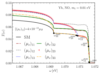
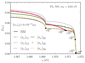
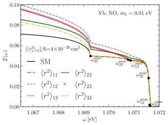
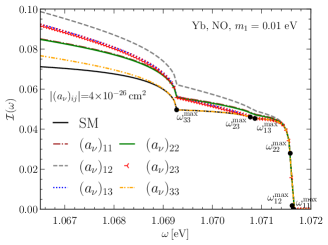
Fig. 1: The spectral function $\mathcal{I}(\omega)$ for the Yb atom RENP processes with weak (SM) and neutrino EM interactions as a function of the trigger laser frequency $\omega$ for the normal ordering (NO) of neutrino masses and the lightest neutrino mass $m_{1}=0.01$ eV.

Comparing the result in Eq. (3.26) with the SM-only case [31, 64, 65, 36],

$$\Gamma_{W} =\Gamma_{0}\sum_{ij}\frac{\Delta_{ij}\Theta(\omega-\omega_{ij}^{\rm max})}{3(E_{vg}-\omega)^{2}}\Biggl{\{}|a_{ij}|^{2}\Bigl{[}q^{2}-\frac{1}{2}(m_{i}^{2}+m_{j}^{2})+\frac{\omega^{2}}{2}\left(1-\frac{1}{3}\Delta_{ij}^{2}\right)$$

$$\hskip 142.26378pt-\frac{(E_{eg}-\omega)^{2}(\Delta m_{ij}^{2})^{2}}{2q^{4}}\Bigr{]}-3\delta_{M}{\rm Re}[a_{ij}^{2}]m_{i}m_{j}\Biggr{\}},$$ (3.28)

the relative size $\Gamma_{\mu}/\Gamma_{W}\sim\omega^{2}\mu_{B}^{2}|(\mu_{\nu})_{ij}|^{2}/G_{F}^{2}q^{2}\sim|(\mu_{\nu})_{ij}|^{2}/[10^{-11}\mu_{B}]^{2}$ scales with $\mu^{2}_{\nu}$ for the magnetic moment and similarly for its electric dipole counterpart. While the SM contribution is mediated by the heavy $W/Z$ bosons, the neutrino magnetic and electric moment contributions are inversely proportional to $1/q^{4}$. With typical $q\sim\mathcal{O}$(eV) for atomic processes, the SM contribution is suppressed by a factor of $(q^{2}/m_{W}^{2})^{2}\sim 10^{-44}$. However the presence of the electron magnetic moment suppresses the EM contribution by $\omega/\mu_{B}\sim 10^{-6}\,$eV. All in all, a $|(\mu_{\nu})_{ij}|\sim 10^{-11}\mu_{B}$ provides similar contribution to that of the SM.

The total spectral function, $\mathcal{I}\equiv\mathcal{I}_{W}+\mathcal{I}_{\mu,\epsilon}$, is presented in the upper left (right) panels of Fig. 1 with the representative value of $|(\mu_{\nu})_{ij}|^{2}$ and $|(\epsilon_{\nu})_{ij}|^{2}$ being $4\times 10^{-11}\,\mu_{B}$. In both cases, the curves significantly differ from the SM contribution (black). The kinks in the curves represents the location of all six frequency thresholds in Eq. (3.12). In all curves, the magnetic moment contribution is slightly larger than the electric dipole one due to the difference in the sign in $m_{j}$. The difference in the shape of $\mathcal{I}$ over the frequency range can be used to experimentally distinguish both contributions.

3.5 Charge Radius and Anapole Contributions

The charge radius and anapole always appear together with similar Lorentz structure,

$$\mathcal{M}_{r,a}=2\mu_{\rm B}(0,{\boldsymbol{s}}_{vg}\times{\boldsymbol{q}})_{\mu}\overline{u}(p_{\nu_{i}})\left(\gamma^{\mu}-\frac{q^{\mu}\not{q}}{q^{2}}\right)\left(\frac{\langle r^{2}_{\nu}\rangle_{ij}}{6}+(a_{\nu})_{ij}\gamma_{5}\right)v(p_{\nu_{j}}).$$ (3.29)

The total matrix element is then $\mathcal{M}_{\nu\bar{\nu}}=\mathcal{M}_{W}+\mathcal{M}_{r,a}$. Similarly to the previous section, the spin averaged matrix element squared contains three terms, the SM-only term, the interference term between SM and EM contributions, as well as the pure charge radius and anapole terms. The interference between $M_{W}^{(D)}$ in Eq. (3.5) and $\mathcal{M}_{r,a}$ is,

$$\overline{\mathcal{M}_{W}^{(D)}\mathcal{M}_{r,a}^{*}}= -\frac{2\sqrt{2}G_{\rm F}\mu_{B}a_{ij}}{2(J_{e}+1)}\sum_{spins}(0,\hat{\boldsymbol{s}}_{vg})^{\nu}(0,{\boldsymbol{s}}_{vg}\times{\boldsymbol{q}})^{\mu}$$

$$\times{\rm Tr}\Biggl{\{}\left(\gamma_{\mu}-\frac{q_{\mu}\not{q}}{q^{2}}\right)\left[\frac{\langle r^{2}_{\nu}\rangle_{ij}^{*}}{6}+(a_{\nu})_{ij}^{*}\gamma_{5}\right](\not{p}_{j}-m_{j})\gamma_{\nu}P_{L}(\not{p}_{i}+m_{i})\Biggr{\}}.$$ (3.30)

The sum over electron spins is performed using the spin relation in Eq. (3.21) to obtain,

$$2{\rm Re}\left[\overline{\mathcal{M}_{W}^{(D)}\mathcal{M}_{r,a}^{*}}\right]=\frac{16\sqrt{2}(2J_{v}+1)C_{ve}\mu_{\rm B}G_{\rm F}}{3}q^{2}{\rm Im}\left[a_{ij}\left(\frac{\langle r^{2}_{\nu}\rangle_{ij}^{*}}{6}-(a_{\nu})_{ij}^{*}\right)\right]\left(E_{\nu_{i}}-\overline{E}\right).$$ (3.31)

with $\overline{E}$ defined in Eq. (3.18). As before, this interference term ${\rm Re}\left[\overline{\mathcal{M}_{W}^{(D)}\mathcal{M}_{r,a}^{*}}\right]\propto\left(E_{\nu_{i}}-\overline{E}\right)$ is an odd function around $\overline{E}$ and hence does not contribute to the total rate after integration over $E_{\nu_{i}}$.

The only contribution from the neutrino charge radius and anapole is the square of Eq. (3.29),

$$\overline{|\mathcal{M}_{r,a}|^{2}}= 4\mu_{\rm B}^{2}\frac{1}{2(2J_{e}+1)}\sum_{\rm spins}(0,{\boldsymbol{s}}_{ev}\times{\boldsymbol{q}})^{\mu}(0,{\boldsymbol{s}}_{ev}^{*}\times{\boldsymbol{q}})^{\nu}{\rm Tr}\Biggl{[}\left(\gamma^{\mu}-\frac{q^{\mu}\not{q}}{q^{2}}\right)$$ (3.32)

$$\left(\frac{\langle r^{2}_{\nu}\rangle_{ij}}{6}+(a_{\nu})_{ij}\gamma_{5}\right)(\not{p}_{\overline{\nu}_{j}}-m_{j})\left(\gamma^{\nu}-\frac{q^{\nu}\not{q}}{q^{2}}\right)\left(\frac{\langle r^{2}_{\nu}\rangle_{ij}}{6}+(a_{\nu})_{ij}^{*}\gamma_{5}\right)(\not{p}_{\nu_{i}}+m_{i})\Biggr{]}.$$

The presence of $\gamma_{5}$ in the anapole term ensures that there is no interference between $\langle r^{2}_{\nu}\rangle_{ij}$ and $(a_{\nu})_{ij}$. After using Eq. (3.21) to eliminate the spin operators, the matrix element squared becomes,

$$\overline{|\mathcal{M}_{{}^{r}_{a}}|^{2}}=\frac{4(\mu_{\rm B}\omega)^{2}}{3}(2J_{v}+1)C_{ve}\Biggl{[}\frac{q^{2}}{2}-\frac{1}{2}(m_{i}\mp m_{j})^{2}+|{\boldsymbol{p}}_{i}|^{2}\sin^{2}\theta\Biggr{]}\begin{cases}\frac{|\langle r^{2}_{\nu}\rangle_{ij}|^{2}}{36},\\[5.0pt] |(a_{\nu})_{ij}|^{2}.\end{cases}$$ (3.33)

The only difference between the charge radius and anapole terms is the minus sign in front of $m_{j}$, which comes from the $\gamma_{5}$ matrix in the anapole interaction. Using the decay rate definition in Eq. (3.19) and the kinematic limits in Eq. (3.17), the total decay rate becomes,

$$\Gamma_{{}^{r}_{a}}=\Gamma_{0}\sum_{ij}\frac{|\mu_{\rm B}|^{2}}{9G_{F}^{2}}\frac{\omega^{2}q^{2}\Delta_{ij}\Theta(\omega-\omega_{ij}^{\rm max})}{(E_{vg}-\omega)^{2}}\left[1-\frac{(m_{i}\mp m_{j})^{2}}{q^{2}}\right]\left[1-\frac{(m_{i}\pm m_{j})^{2}}{4q^{2}}\right]\begin{cases}\frac{|\langle r^{2}_{\nu}\rangle_{ij}|^{2}}{36},\\[5.0pt] |(a_{\nu})_{ij}|^{2},\end{cases}$$ (3.34)

where $\Gamma_{0}$ is defined in Eq. (3.27) and the step function $\Theta(\omega-\omega_{ij}^{\rm max})$ defines the frequency thresholds of Eq. (3.12). The relative size between the SM contribution in Eq. (3.28) and the anapole term is $\Gamma_{a}/\Gamma_{W}\sim\mu_{B}^{2}\omega^{2}|(a_{\nu})_{ij}|^{2}/3G_{F}^{2}\sim\left(\omega/{\rm eV}\right)^{2}\left(|(a_{\nu})_{ij}|/10^{-26}{\rm cm}^{2}\right)^{2}$. With the expectation that the sensitivity is projected for the signal to have roughly the same event rate as the SM background, the neutrino charge radius and anapole can be probed at the level of $10^{-26}{\rm cm}^{2}$. Notice that an experiment with higher trigger frequency $\omega$ provides larger sensitivity on the charge radius and anapole due to the $\omega^{2}$ factor.

The total spectral function $\mathcal{I}\equiv\mathcal{I}_{W}+\mathcal{I}_{r,a}$ is presented in the bottom left (right) panels of Fig. 1 for the representative value of $|\langle r^{2}_{\nu}\rangle_{ij}|/6$ and $|(a_{\nu})_{ij}|$ of $4\times 10^{-26}$ cm². In both cases, the curves significantly differ from the SM contribution specially for lower frequencies. In all curves, the charge radius contribution is slightly larger than the anapole one due to the difference in the sign in $m_{j}$, which modified $(m_{i}\pm m_{j})^{2}/q^{2}$ in Eq. (3.34). Since $q^{2}=E_{eg}^{2}-2E_{eg}\omega$ decreases with increasing frequency, the relative difference between the charge radius and anapole curves becomes larger for higher frequency. In the next section, we show that the difference in the shape of $\mathcal{I}_{r}$ and $\mathcal{I}_{a}$ can be used to experimentally distinguish them.

4 RENP Sensitivity to Neutrino EM Properties

The advantage of RENP is its capability of separating the individual form factor elements $f^{ij}_{M,E,Q,A}$ of Eq. (2.3) as first noticed in [29]. From the hermiticity condition, each form factor contains 6 elements that enter the spectral function as magnitudes squared $|f^{ij}_{M,E,Q,A}|^{2}$ while their phases do not appear. The kinematics in Sec. 3.4 allows the photon energy up to certain threshold frequency $\omega^{ij}_{\rm max}$ defined in Eq. (3.12) for each neutrino pair $\nu_{i}\bar{\nu}_{j}$. With the trigger laser having a precision of $\delta\omega\sim 10^{-5}$ eV [31] which is much better than $E_{eg}/2-\omega_{ij}^{\rm max}\sim 10^{-5}-10^{-3}$ eV, it is possible to scan the various thresholds $\omega_{ij}^{\rm max}$ with different combinations of neutrino mass eigenvalues and the regions in between. Scanning over 6 frequencies is sufficient to separate individual matrix elements as proposed in [29]. For illustration, we take $\omega_{i}=(1.069$, 1.07, 1.0708, 1.0712, 1.0716, 1.07164) eV shown as the black points in Fig. 2.

Once nonzero deviation from the SM prediction is observed, the experiment is also capable of identifying which neutrino property ($\mu_{\nu}$, $\epsilon_{\nu}$, $\langle r^{2}_{\nu}\rangle$, or $a_{\nu}$) is contributing. If one element with specific indices $i$ and $j$ is experimentally observed to be nonzero, the spectrum function below the corresponding $\omega^{\rm max}_{ij}$ is affected and can be scanned to identify which type that element is. At least another 3 frequency points are necessary to reconstruct the photon spectrum and then identify the relevant neutrino property. Since the spectrum function has larger value for smaller $\omega$, we choose the three frequencies $\omega_{i}=(1.0672$, 1.0678, 1.0684) eV shown as red points in Fig. 2 to increase event rate. Another reason of choosing lower frequencies bellow all $\omega^{\rm max}_{ij}$ is that all elements can contribute to this region. However, if the nonzero element has larger $\omega^{\rm max}_{ij}$, it is also advantageous to add more frequency points. Both the low and high frequency regions are sensitive to distinguishing $\langle r^{2}_{\nu}\rangle_{12}$ and $(a_{\nu})_{12}$ from $(\mu_{\nu})_{12}$ and $(\epsilon_{\nu})_{12}$ with apparent difference. The difference between $(\mu_{\nu})_{12}$ and $(\epsilon_{\nu})_{12}$ is also larger at the high frequency region.

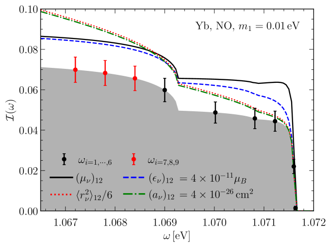
Fig. 2: The spectral function $\mathcal{I}(\omega)$ for the Yb atom RENP process considering SM background only (gray area), the neutrino magnetic/electric moment $(\mu_{\nu})_{12}=4\times 10^{-11}\mu_{B}$ (black line), $(\epsilon_{\nu})_{12}=4\times 10^{-11}\mu_{B}$ (blue dashed line), $\langle r^{2}_{\nu}\rangle_{12}=2.4\times 10^{-25}$ cm² (red dotted line), and $(a_{\nu})_{12}=4\times 10^{-26}$ cm² (green dashed-dotted line) in the normal ordering (NO) case with $m_{1}=0.01$ eV. We also show the 6 frequencies (black dots) needed to separate the matrix elements and the other 3 frequencies (red dots) for identifying the form factor type.

Following the setup in [29], we estimate the number of RENP photons at each frequency $\omega$ as $N_{i}=T\Gamma_{0}\mathcal{I}(\omega_{i})$,

$$N_{i}\approx 173\left(\frac{T}{\rm days}\right)\left(\frac{V}{100~{}\rm cm^{3}}\right)\left(\frac{n_{a}~{}{\rm or}~{}n_{\gamma}}{10^{21}\rm cm^{-3}}\right)^{3}\mathcal{I}(\omega_{i}),$$ (4.1)

where $T$ is the exposure time that we take to be equal among all the nine $\omega_{i}$ values. While $V$ is the target volume, $\mathcal{I}(\omega)$ is the total spectral function containing the SM and EM contributions. For a typical Yb experiment with $T=10$ days, we expect $N(\omega_{i=1,\dots,9})=(146$, 136, 120, 107, 87, 82, 79, 39, 2.5) SM background events, respectively, and in total 759 events. The sensitivity is evaluated using the Poisson $\chi^{2}$ function,

$$\Delta\chi^{2}\equiv 2\sum_{i=1}^{9}\Bigl{\{}N^{\rm true}_{i}-N^{\rm test}_{i}-N^{\rm true}_{i}\log\left[N^{\rm true}_{i}/N^{\rm test}_{i}\right]\Bigr{\}},\quad$$ (4.2)

where $N^{\rm true}_{i}$ ($N^{\rm test}_{i}$) are the event numbers with SM only (SM and EM) contributions at each frequency $\omega_{i}$. Fig. 3 shows the 90% C.L. ($\Delta\chi^{2}=2.71$) sensitivity for individual matrix elements as a function of the total number of events. For comparison, we also show the existing constraints from the reactor experiment TEXONO [16] (blue dotted line), the solar neutrino measurement [55, 18] (purple dotted line), and the stellar cooling with plasmon decay for red giants (RG) [26] (red dotted lines) or white dwarfs (WD) [24, 25] (yellow dotted lines) as discussed in Sec. 2.2. The sensitivity of $\mu_{\nu}$ reaches the direct detection experiment sensitivity of $3\times 10^{-11}\mu_{B}$ at 1000 events while it takes twice for $\epsilon_{\nu}$ to reach the same value.

As expected from the discussions in Sec. 3.5, the sensitivity for charge radius and anapole is around $10^{-26}$ cm² which is 5 orders of magnitude smaller than the existing constraints. However, the existing constraints are on combinations of various matrix elements and hence subject to parameter degeneracies. With much stronger constraints on parameter combinations, the individual elements can still be sizable. The only exception is stellar cooling whose constraint is on the sum of matrix elements squared. However, the stellar cooling calculation suffers from large theoretical uncertainties. The RENP experiment can provide unique capability of identifying individual elements and their type. We can also expect further sensitivity improvement if the E1$\times$E1 configuration is adopted.

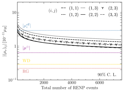
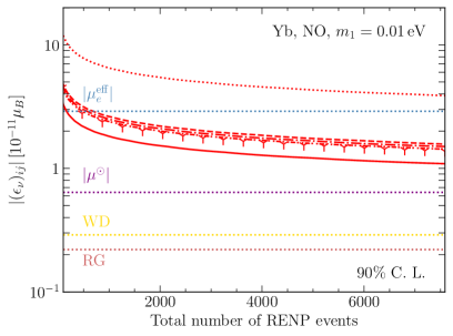
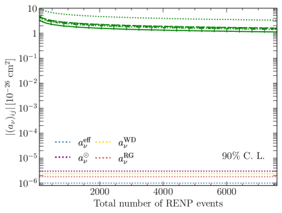
Fig. 3: The expected sensitivities to neutrino electromagnetic form factors at 90% C.L. as a function of the expected event rate for $(\mu_{\nu})_{ij}$ (top left), $(\epsilon_{\nu})_{ij}$ (top right), $\langle r_{\nu}^{2}\rangle_{ij}$ (bottom left), and $(a_{\nu})_{ij}$ (bottom right) with the normal ordering (NO) and $m_{1}=0.01$ eV. The dotted lines show the current bounds on the effective parameters from reactor (dotted blue for $\mu_{e}^{\rm eff}$ or $\langle r_{\nu}^{2}\rangle^{\rm eff}$) [16] and solar (dotted purple for $\mu_{e}^{\odot}$ or $\langle r_{\nu}^{2}\rangle^{\odot}$) [55, 18] neutrinos, as well as plasmon decay in red giants (dotted red for RG) [26] and white dwarfs (dotted yellow for WD) [24, 25].

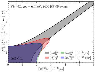
Fig. 4: Left : The $\sqrt{\Delta\chi^{2}}$ profile for a non-zero neutrino magnetic moment $(\mu_{\nu})_{12}^{\rm true}=4\times 10^{-11}\,\mu_{B}$. Right: The allowed regions as a function of $(\mu_{\nu})_{12}^{\rm true}\in[0,6]\times 10^{-11}\,\mu_{B}$. In total 1000 events are used for illustration. The regions represents several test models: $(\mu_{\nu})_{12}^{\rm test}$ free (black), $(\epsilon_{\nu})_{12}^{\rm test}$ free (red dashed), $\langle r_{\nu}^{2}\rangle_{12}^{\rm test}$ free (blue dotted), and $(a_{\nu})_{12}^{\rm test}$ free (green dot-dashed).

To illustrate the RENP capability of distinguishing the neutrino form factors, the left panel of Fig. 4 shows the $\Delta\chi^{2}$ for $(\mu_{\nu})_{12}^{\rm true}=4\times 10^{-11}\,\mu_{B}$ when compared with the fit for $(\mu_{\nu})_{12}^{\rm test}$, $(\epsilon_{\nu})_{12}^{\rm test}$, $\langle r_{\nu}^{2}\rangle_{12}^{\rm test}$, or $(a_{\nu})_{12}^{\rm test}$ with the same indices $i=1$ and $j=2$. Since the decay rate is proportional to the coupling constant squared, all the curves have two local minimums with just a sign difference. While the black curve with $(\mu_{\nu})^{\rm test}_{12}$ as fitting variable can touch the horizontal axis, the other three curves have nonzero $\chi^{2}_{\rm min}$. A non-zero $\Delta\chi^{2}$ minimum excludes the coupling by $\sqrt{\Delta\chi^{2}}$ standard deviation. Both charge radius and anapole can be excluded by $\sim 6.5\,\sigma$ while the neutrino EDM by $4\,\sigma$ with 1000 RENP events ($T=10$ days). The higher exclusion sensitivity for $\langle r_{\nu}^{2}\rangle_{12}$ and $(a_{\nu})_{12}$ than the $(\epsilon_{\nu})_{12}$ one is expected since the shape of the EDM spectral function is closer to the magnetic moment one. The difference is especially significant at the lower frequency region that contains more events and larger deviation as pointed above.

The right panel of Fig. 4 shows the sensitivity on the neutrino form factors as a function of the true value $(\mu_{\nu})_{12}^{\rm true}$ with the 90% C.L. upper/lower limits on the test form factor elements that are shown as the $y$-axis. For a nonzero $(\mu_{\nu})_{12}^{\rm true}$, only the test magnetic moment has upper and lower bounds $(\mu_{\nu})_{12}^{\rm test}\pm\Delta\mu_{\nu}$ when $(\mu_{\nu})_{12}^{\rm true}>3\times 10^{-11}\mu_{B}$. Conversely, the EDM parameter space cannot explain the data at 90% C.L. for $(\mu_{\nu})_{12}^{\rm true}>3\times 10^{-11}\mu_{B}$ and has only an upper bound if $(\mu_{\nu})_{12}^{\rm true}<2\times 10^{-11}\mu_{B}$. Since the charge radius and anapole curves are significantly different from the magnetic moment one, they cannot explain the data at 90% C.L. for $(\mu_{\nu})_{12}^{\rm true}>2.4\times 10^{-11}\mu_{B}$.

5 Discussion & Conclusion

The EM properties are not just the first neutrino interaction that was originally proposed by Pauli in exactly the same letter where he pointed out the existence of neutrino, but can also have sizable values to appear in various BSM models. Hence, observing the neutrino EM properties (magnetic and electric moments, charge radius, and anapole) can serve as a window of probing possible new physics. Unique probe and identification of each form factor elements are necessary which is a serious challenge for the existing experimental measurements and observations. We show that the RENP process is an ideal probe. The typically eV scale momentum transfer of atomic transitions is perfect for probing light mediators including the massless photon. Most importantly, the RENP process do not suffer from degeneracies in EM form factors and hence has the possibility of individual identification as a unique feature. Both analytical derivations and practical searching strategies are provided with great details in the current paper. In addition, the selection rules for the QED double photon emission, the RENP with weak interactions, and the one with neutrino EM properties are systematically derived. While the RENP with weak interactions is dominated by the M1 transition, its counterpart with neutrino EM form factors is actually similar to the QED photon emission that is mainly contributed by the E1 transition. In other words, the bounds can be probably further improved if a RENP experiment can be done with E1$\times$E1 type atomic transitions instead of the usual proposal with E1$\times$M1 transitions.

Appendix A Atomic Transitions with QED and EW Interactions

A.1 Non-Relativistic Electron Hamiltonian

Here we start from first principles and obtain the complete Hamiltonian for a non-relativistic bound electron. It is more convenient to add the electron QED and EW interactions in terms of Lagrangian,

$$\mathcal{L}_{EW}=\overline{e}\left[i\not{\partial}-e\not{A}-\sqrt{2}G_{\rm F}\not{j}^{(\nu)}\left(v+a\gamma_{5}\right)-m_{e}\right]e+\dots,$$ (A.1)

where $j^{(\nu)}_{\mu}\equiv\bar{\nu}\gamma_{\mu}P_{L}\nu$ is the neutrino current. Note that the chiral coefficients $v$ and $a$ are attached to the electron bilinears. The Dirac equation for the electron field $e(x)$ in the presence of a photon field $A_{\mu}$ and a neutrino current is,

$$\left[i\partial_{\mu}+(J_{V})_{\mu}-(J_{A})_{\mu}\gamma_{5}\right]\gamma^{\mu}e(x)=m_{e}e(x).$$ (A.2)

For convenience, we define the two effective vector and axial currents, respectively, as

$$(J_{V})_{\mu}\equiv-eA_{\mu}-\sqrt{2}vG_{\rm F}j^{(\nu)}_{\mu},\quad{\rm and}\quad(J_{A})_{\mu}\equiv-\sqrt{2}aG_{\rm F}j^{(\nu)}_{\mu}.$$ (A.3)

In the non-relativistic limit, the four-component electron spinor would reduce to its two-component counterpart that people are usually familiar with in quantum mechanics while the other two components are suppressed. This feature becomes more transparent in the Dirac representation,

$$\gamma^{0}_{D}=\left(\begin{matrix}1&0\\ 0&-1\end{matrix}\right),\quad\gamma^{i}_{D}=\left(\begin{matrix}0&-\sigma^{i}\\ \sigma^{i}&0\end{matrix}\right),\quad{\rm and}\quad\gamma^{5}_{D}=\left(\begin{matrix}0&1\\ 1&0\end{matrix}\right).$$ (A.4)

Correspondingly, the electron field splits into two two-component spinors, $e(x)\equiv(\psi({\boldsymbol{x}}),\phi({\boldsymbol{x}}))$ $e^{-iEt}$, with $E$ being the total energy [69]. Since our discussions in this paper focus on only the electron particle and do not touch positron, only the positive-frequency mode needs to be considered for simplicity. While the time dependence can be factorized out with $e^{-iEt}$, the spatial distribution of the bound electron field in an atom is nontrivial and will be elaborated below. Putting the electron field $e(x)$ back into Eq. (A.2) allows us to obtain two coupled equations for $\psi$ and $\phi$,

$$\left[(i\boldsymbol{\nabla}+{\boldsymbol{J}}_{V})\cdot\boldsymbol{\sigma}+J_{A}^{0}\right]\phi=-\left[E-m_{e}+J_{V}^{0}+({\boldsymbol{J}}_{A}\cdot\boldsymbol{\sigma})\right]\psi\,,$$ (A.5a)

$$\left[(i\boldsymbol{\nabla}+{\boldsymbol{J}}_{V})\cdot\boldsymbol{\sigma}+J^{0}_{A}\right]\psi=-\left[E+m_{e}+J_{V}^{0}+({\boldsymbol{J}}_{A}\cdot\boldsymbol{\sigma})\right]\phi\,.$$ (A.5b)

Notice that the crucial signs of $E-m_{e}$ in the first equation and $E+m_{e}$ in the second one make big difference. For a non-relativistic electron ($|{\boldsymbol{p}}_{e}|$, $J_{V}^{0}$, and ${\boldsymbol{J}}_{A}\cdot\boldsymbol{\sigma}\ll m_{e}$), it follows from the second equation above that, $\phi/\psi\sim\mathcal{O}\left(|{\boldsymbol{p}}_{e}|/m_{e}\right)$. Consequently, the electron wave function is given mostly by $\psi$ while the $\phi$ obtained from Eq. (A.5b),

$$\phi\approx-\frac{1}{2m_{e}}\left[(i\boldsymbol{\nabla}+{\boldsymbol{J}}_{V})\cdot\boldsymbol{\sigma}+J^{0}_{A}\right]\psi,$$ (A.6)

is highly suppressed.

For convenience, we redefine the total energy $E$ as $E\equiv m_{e}+E^{\rm NR}$, with $E^{\rm NR}\ll m_{e}$. The quantity $E^{\rm NR}$ is the non-relativistic energy of the electron. For a free electron, $E^{\rm NR}=T_{e}\approx|{\boldsymbol{p}}_{e}|^{2}/2m_{e}$. However, in the presence of interacting fields $E^{\rm NR}$ represents not only the electron kinetic energy ($T_{e}$), but contains potential terms related to $J_{V}$ and $J_{A}$, as will become evident below. Using the above approximation Eq. (A.6) to substitute $\phi$ back into the left-hand side of Eq. (A.5a) and keeping the leading order in $m_{e}^{-1}$, we obtain the non-relativistic electron Schrödinger equation,

$$\left\{\frac{1}{2m_{e}}\left[(i\boldsymbol{\nabla}+{\boldsymbol{J}}_{V})\cdot\boldsymbol{\sigma}+J_{A}^{0}\right]^{2}-J_{V}^{0}-({\boldsymbol{J}}_{A}\cdot\boldsymbol{\sigma})\right\}\psi=E^{\rm NR}\psi\,.$$ (A.7)

In other words, the electron Hamiltonian with both QED and EW interactions is,

$$H_{EW}\equiv\frac{1}{2m_{e}}\left[(i\boldsymbol{\nabla}+{\boldsymbol{J}}_{V})\cdot\boldsymbol{\sigma}+J_{A}^{0}\right]^{2}-J_{V}^{0}-({\boldsymbol{J}}_{A}\cdot\boldsymbol{\sigma}).$$ (A.8)

The first term is a kinetic energy in the presence of vector/pseudo-vector fields while the last two terms are the potential energy.

For later convenience, we reformulate the Hamiltonian as,

$$H_{EW} =\frac{1}{2m_{e}}\left[(i\boldsymbol{\nabla}+{\boldsymbol{J}}_{V})^{2}+2J_{A}^{0}\boldsymbol{\sigma}\cdot(i\boldsymbol{\nabla}+{\boldsymbol{J}}_{V})+i\boldsymbol{\sigma}\cdot(\boldsymbol{\nabla}J_{A}^{0})+(J_{A}^{0})^{2}-\boldsymbol{\sigma}\cdot(\boldsymbol{\nabla}\times{\boldsymbol{J}}_{V})\right]$$ (A.9a)

$$-J_{V}^{0}-{\boldsymbol{J}}_{A}\cdot\boldsymbol{\sigma},$$ (A.9b)

by using the identity $(\boldsymbol{\sigma}\cdot{\boldsymbol{A}})(\boldsymbol{\sigma}\cdot{\boldsymbol{B}})={\boldsymbol{A}}\cdot{\boldsymbol{B}}+i\boldsymbol{\sigma}\cdot({\boldsymbol{A}}\times{\boldsymbol{B}})$. The total Hamiltonian can split into three parts,

$$H_{EW}\equiv H_{0}+H_{\gamma}+H_{\nu\bar{\nu}},$$ (A.10)

for describing the atomic energy levels, the atomic transitions, and the radiative emission of neutrino pair as we elaborate below.

A.2 Atomic Energy Levels and Transition with QED

The Hamiltonian in Eq. (A.9) can in principle describe any vector and axial-vector interactions. For electromagnetic coupling with photon, $J_{V}^{0}=-eA_{0}=-eV(x)$ and ${\boldsymbol{J}}_{V}=-e{\boldsymbol{A}}$. To be exact, $J_{V}^{0}$ is the electric potential due to the electron charge and $\boldsymbol{\nabla}\times{\boldsymbol{J}}_{V}=-e\boldsymbol{\nabla}\times{\boldsymbol{A}}$ is actually the magnetic field coupled with electron spin.

The photon field has two contributions, $A_{\mu}\equiv A^{(0)}_{\mu}+A^{(\gamma)}_{\mu}$, a classical EM field $A^{(0)}_{\mu}$ as background generated by the atomic charges and a quantum fluctuation component for photon emission/absorption $A^{(\gamma)}_{\mu}$. Of these two components, the quantum part $A^{(\gamma)}_{\mu}$ is usually treated as radiative perturbations while the classical one $A^{(0)}_{\mu}$ forms the atomic Hamiltonian, $H_{0}$, that describes the atomic energy levels, $H_{0}|a\rangle=E_{a}|a\rangle$ with $a=g$, $e$, and $v$ for the ground, excited, and intermediate virtual states. To be more concrete, $H_{0}$ is a combination of the electron kinetic energy and the classical electromagnetic potential obtained by replacements $J_{V}\rightarrow-eA^{(0)}$ and $J_{A}\rightarrow 0$ from Eq. (A.9),

$$H_{0}\equiv-\frac{\boldsymbol{\nabla}^{2}}{2m_{e}}-\frac{ie}{2m_{e}}\left(2{\boldsymbol{A}}^{(0)}\cdot\boldsymbol{\nabla}+\boldsymbol{\nabla}\cdot{\boldsymbol{A}}^{(0)}\right)+\frac{e^{2}}{2m_{e}}({\boldsymbol{A}}^{(0)})^{2}+\frac{e\boldsymbol{\sigma}}{2m_{e}}\cdot(\boldsymbol{\nabla}\times{\boldsymbol{A}}^{(0)})+eA_{0}^{(0)}.\quad$$ (A.11)

Since $A^{(\gamma)}$ is a small perturbation, one needs to keep only the linear terms of $A^{(\gamma)}$ for the photon emission Hamiltonian $H_{\gamma}$,

$$H_{\gamma} \equiv eA^{(\gamma)}_{0}-\frac{e}{m_{e}}{\boldsymbol{A}}^{(\gamma)}\cdot(i\boldsymbol{\nabla}-e{\boldsymbol{A}}^{(0)})-\frac{ie}{2m_{e}}\boldsymbol{\nabla}\cdot{\boldsymbol{A}}^{(\gamma)}+\frac{e}{2m_{e}}\boldsymbol{\sigma}\cdot(\boldsymbol{\nabla}\times{\boldsymbol{A}}^{(\gamma)}).$$ (A.12)

Since the single-photon emission ($|i\rangle\rightarrow|f\rangle+\gamma$) happens between two different atomic states ($|i\rangle$ for the initial and $|f\rangle$ for the final), the trivially multiplicative operators $eA^{(\gamma)}_{0}$ and $ie\boldsymbol{\nabla}\cdot{\boldsymbol{A}}^{(\gamma)}/2m_{e}$ cannot contribute due to orthogonality of atomic states. For example, $\langle i|eA^{(\gamma)}_{0}|f\rangle=eA^{(\gamma)}_{0}\langle i|f\rangle=0$. Although the electric potential $eA^{(\gamma)}_{0}$ contributes mainly for determining the atomic energy levels but not the transition among them. So finally there are only two terms remaining.

The term $i\boldsymbol{\nabla}-e{\boldsymbol{A}}^{(0)}$ is related to the position operator $\hat{\boldsymbol{x}}$ via $i\boldsymbol{\nabla}-e{\boldsymbol{A}}^{(0)}=im_{e}[\hat{\boldsymbol{x}},H_{0}]$. With this replacement, the photon emission Hamiltonian becomes,

$$H_{\gamma} =-ie{\boldsymbol{A}}^{(\gamma)}\cdot[\hat{\boldsymbol{x}},H_{0}]+\frac{e}{2m_{e}}\boldsymbol{\sigma}\cdot(\boldsymbol{\nabla}\times{\boldsymbol{A}}^{(\gamma)}).$$ (A.13)

The first is proportional to the space coordinate operator $\hat{\boldsymbol{x}}$ and hence contributes as dipole operator, ${\boldsymbol{d}}_{if}\propto\langle i|\hat{\boldsymbol{x}}|f\rangle$. On the other hand, the second term contains the electron spin operator ($\hat{\boldsymbol{s}}=\boldsymbol{\sigma}/2$) and the magnetic field ($\boldsymbol{B}=\boldsymbol{\nabla}\times A^{(\gamma)}$). Both terms are contributed by the three-dimensional vector potential $\boldsymbol{A}^{(\gamma)}$.

The two terms in Eq. (A.13) have definite spin and parity such that the induced transitions are subject to handy selection rules for the single-photon emission, $|i\rangle\rightarrow|f\rangle+\gamma$. The total angular momentum from the initial ($J_{i}$) to the final one ($J_{f}$) changes by at most one single unity, $J_{f}-J_{i}=0$, $\pm 1$, with the $J_{i}=J_{f}=0$ transition also forbidden. At the same time, the magnetic quantum number should also change at most by one unity, $M_{J_{i}}-M_{J_{f}}=0$, $\pm 1$. The relative parity between the initial ($\pi_{e}$) and final ($\pi_{g}$) states determines if the transition is E1 type with parity flip ($\pi_{f}=-\pi_{i}$) or M1 type with parity conserved ($\pi_{f}=\pi_{i}$). Since the dipole operator reverses sign under parity transformation, $\hat{\boldsymbol{x}}\rightarrow-\hat{\boldsymbol{x}}$, it induces E1 type transition while the magnetic moment operator in the second term of Eq. (A.13) is M1 type.

The two terms in Eq. (A.13) have different typical sizes. The dipole term is in unit of the Bohr radius $a_{0}=(m_{e}\alpha)^{-1}$ while the magnetic moment operator is regulated by the Bohr magneton ($\mu_{B}=e/2m_{e}$) which is suppressed by the electron mass. Although the dipole term also contains $H_{0}$ that gives the atomic energy at $\mathcal{O}($eV), the $\boldsymbol{\nabla}$ operator in the magnetic moment operator gives the photon frequency which is also at eV scale to balance. Consequently, the E1 transition is typically $\alpha^{-1}\sim 100$ times larger than its M1 counterpart.

A.3 Radiative Emission of Neutrino Pair with EW

The remaining terms in the Hamiltonian of Eq. (A.10) are responsible for the neutrino pair emission, $|e\rangle\rightarrow|v\rangle+\nu\bar{\nu}$,

$$H_{\nu\bar{\nu}} =-i\sqrt{2}G_{\rm F}\left(v{\boldsymbol{j}}^{(\nu)}+aj_{0}^{(\nu)}\boldsymbol{\sigma}\right)\cdot[\hat{\boldsymbol{x}},H_{0}]+\sqrt{2}G_{\rm F}(vj^{(\nu)}_{0}+a{\boldsymbol{j}}^{(\nu)}\cdot\boldsymbol{\sigma})$$ (A.14a)

$$+\frac{vG_{\rm F}}{\sqrt{2}m_{e}}\boldsymbol{\sigma}\cdot(\boldsymbol{\nabla}\times{\boldsymbol{j}}^{(\nu)})-\frac{iG_{\rm F}}{\sqrt{2}m_{e}}\boldsymbol{\nabla}\cdot\left(v{\boldsymbol{j}}^{(\nu)}+aj_{0}^{(\nu)}\boldsymbol{\sigma}\right).$$ (A.14b)

While those terms in the second line are suppressed by the electron mass, any meaningful contribution arises from those in the first line. Due to orthogonality, the $\sqrt{2}G_{\rm F}vj^{(\nu)}_{0}$ term does not contribute to the atomic transition. Among the remaining three terms, $v{\boldsymbol{j}}^{(\nu)}\cdot[\hat{\boldsymbol{x}},H_{0}]$ with dipole operator is E1 type while $a{\boldsymbol{j}}^{(\nu)}\cdot\boldsymbol{\sigma}$ with spinor operator is M1 type. Contrary to the QED emissions discussed above, the neutrino pair M1 emission is not suppressed by the electron mass and hence is around 3 orders ($\sim E_{ve}/\alpha m_{e}$ as a product of the atomic energies and the Bohr radius) of magnitude larger than its E1 counterpart. In other words, the leading photon emission is E1 type while the leading neutrino pair emission is M1 type. Finally, the $aj^{(\nu)}_{0}\boldsymbol{\sigma}\cdot[\hat{\boldsymbol{x}},H_{0}]$ term is a product of the magnetic moment and dipole operators which is at most of the same size as the E1 type and hence subleading.

References

- [1] W. Pauli, “On the Earlier and more recent history of the neutrino,” pages 193-217 of “Writings on Physics and Philosophy”, 978-3-54-056859-9, 978-0-387-56859-1, 978-3-64-208163-7, 978-3-66-202994-7, Springer-Verlag, January 1994
- [2] J. F. Nieves, “Electromagnetic Properties of Majorana Neutrinos,” Phys. Rev. D 26 (1982), 3152.
- [3] B. Kayser, “Majorana Neutrinos and their Electromagnetic Properties,” Phys. Rev. D 26 (1982), 1662.
- [4] R. L. Workman et al. [Particle Data Group], “Review of Particle Physics,” PTEP 2022, 083C01 (2022).
- [5] M. Dvornikov and A. Studenikin, “Electric charge and magnetic moment of massive neutrino,” Phys. Rev. D 69 (2004), 073001 [arXiv:hep-ph/0305206 [hep-ph]].
- [6] J. Bernabeu, L. G. Cabral-Rosetti, J. Papavassiliou and J. Vidal, “On the charge radius of the neutrino,” Phys. Rev. D 62 (2000), 113012 [arXiv:hep-ph/0008114 [hep-ph]].
- [7] K. Fujikawa and R. Shrock, “The Magnetic Moment of a Massive Neutrino and Neutrino Spin Rotation,” Phys. Rev. Lett. 45 (1980), 963.
- [8] P. B. Pal and L. Wolfenstein, “Radiative Decays of Massive Neutrinos,” Phys. Rev. D 25 (1982), 766.
- [9] R. E. Shrock, “Electromagnetic Properties and Decays of Dirac and Majorana Neutrinos in a General Class of Gauge Theories,” Nucl. Phys. B 206 (1982), 359-379.
- [10] A. Studenikin, “Neutrino magnetic moment: A Window to new physics,” Nucl. Phys. B Proc. Suppl. 188 (2009), 220-222 [arXiv:0812.4716 [hep-ph]].
- [11] H. Novales-Sanchez, A. Rosado, V. Santiago-Olan and J. J. Toscano, “Effects of physics beyond the standard model on the neutrino charge radius: an effective Lagrangian approach,” Phys. Rev. D 78 (2008), 073014 [arXiv:0805.4177 [hep-ph]].
- [12] V. Brdar, A. Greljo, J. Kopp and T. Opferkuch, “The Neutrino Magnetic Moment Portal,” [arXiv:2105.06846 [hep-ph]].
- [13] P. Vilain et al. [CHARM-II], “Experimental study of electromagnetic properties of the muon-neutrino in neutrino - electron scattering,” Phys. Lett. B 345 (1995), 115-118.
- [14] L. B. Auerbach et al. [LSND], “Measurement of electron - neutrino - electron elastic scattering,” Phys. Rev. D 63 (2001), 112001 [arXiv:hep-ex/0101039 [hep-ex]].
- [15] R. Schwienhorst et al. [DONUT], “A New upper limit for the tau - neutrino magnetic moment,” Phys. Lett. B 513 (2001), 23-29 [arXiv:hep-ex/0102026 [hep-ex]].
- [16] M. Deniz et al. [TEXONO], “Measurement of Nu(e)-bar -Electron Scattering Cross-Section with a CsI(Tl) Scintillating Crystal Array at the Kuo-Sheng Nuclear Power Reactor,” Phys. Rev. D 81 (2010), 072001 [arXiv:0911.1597 [hep-ex]].
- [17] D. W. Liu et al. [Super-Kamiokande], “Limits on the neutrino magnetic moment using 1496 days of Super-Kamiokande-I solar neutrino data,” Phys. Rev. Lett. 93 (2004), 021802 [arXiv:hep-ex/0402015 [hep-ex]].
- [18] M. Agostini et al. [Borexino], “Limiting neutrino magnetic moments with Borexino Phase-II solar neutrino data,” Phys. Rev. D 96 (2017) no.9, 091103 [arXiv:1707.09355 [hep-xp]].
- [19] E. Aprile et al. [XENON], “Excess electronic recoil events in XENON1T,” Phys. Rev. D 102 (2020) no.7, 072004 [arXiv:2006.09721 [hep-ex]].
- [20] X. Zhou et al. [PandaX-II], “A Search for Solar Axions and Anomalous Neutrino Magnetic Moment with the Complete PandaX-II Data,” Chin. Phys. Lett. 38 (2021) no.1, 011301 [arXiv:2008.06485 [hep-ex]]. [erratum: Chin. Phys. Lett. 38 (2021) no.10, 109902]
- [21] M. Atzori Corona, W. M. Bonivento, M. Cadeddu, N. Cargioli and F. Dordei, “New constraint on neutrino magnetic moment and neutrino millicharge from LUX-ZEPLIN dark matter search results,” Phys. Rev. D 107 (2023) no.5, 053001 [arXiv:2207.05036 [hep-ph]].
- [22] G. G. Raffelt, “Limits on neutrino electromagnetic properties: An update,” Phys. Rept. 320 (1999), 319-327
- [23] A. Mirizzi, D. Montanino and P. D. Serpico, “Revisiting cosmological bounds on radiative neutrino lifetime,” Phys. Rev. D 76 (2007), 053007 [arXiv:0705.4667 [hep-ph]].
- [24] M. M. Miller Bertolami, “Limits on the neutrino magnetic dipole moment from the luminosity function of hot white dwarfs,” Astron. Astrophys. 562, A123 (2014) [arXiv:1407.1404 [hep-ph]].
- [25] B. M. S. Hansen, H. Richer, J. Kalirai, R. Goldsbury, S. Frewen and J. Heyl, “Constraining Neutrino Cooling using the Hot White Dwarf Luminosity Function in the Globular Cluster 47 Tucanae,” Astrophys. J. 809, no.2, 141 (2015) [arXiv:1507.05665 [astro-ph.SR]].
- [26] S. A. Díaz, K. P. Schröder, K. Zuber, D. Jack and E. E. B. Barrios, “Constraint on the axion-electron coupling constant and the neutrino magnetic dipole moment by using the tip-RGB luminosity of fifty globular clusters,” [arXiv:1910.10568 [astro-ph.SR]].
- [27] W. Grimus and P. Stockinger, “Effects of neutrino oscillations and neutrino magnetic moments on elastic neutrino - electron scattering,” Phys. Rev. D 57, 1762-1768 (1998) [arXiv:hep-ph/9708279 [hep-ph]].
- [28] D. Aristizabal Sierra, O. G. Miranda, D. K. Papoulias and G. S. Garcia, “Neutrino magnetic and electric dipole moments: From measurements to parameter space,” Phys. Rev. D 105 (2022) no.3, 035027 [arXiv:2112.12817 [hep-ph]].
- [29] S. F. Ge and P. Pasquini, “Unique probe of neutrino electromagnetic moments with radiative pair emission,” Phys. Lett. B 841 (2023), 137911 [arXiv:2206.11717 [hep-ph]].
- [30] M. Yoshimura, “Neutrino Pair Emission from Excited Atoms,” Phys. Rev. D 75 (2007), 113007 [ arXiv:hep-ph/0611362 [hep-ph]].
- [31] D. N. Dinh, S. T. Petcov, N. Sasao, M. Tanaka and M. Yoshimura, “Observables in Neutrino Mass Spectroscopy Using Atoms,” Phys. Lett. B 719, 154-163 (2013) [ arXiv:1209.4808 [hep-ph]].
- [32] A. Fukumi, S. Kuma, Y. Miyamoto, K. Nakajima, I. Nakano, H. Nanjo, C. Ohae, N. Sasao, M. Tanaka and T. Taniguchi, et al. “Neutrino Spectroscopy with Atoms and Molecules,” PTEP 2012, 04D002 (2012) [ arXiv:1211.4904 [hep-ph]].
- [33] D. N. Dinh and S. T. Petcov, “Radiative Emission of Neutrino Pairs in Atoms and Light Sterile Neutrinos,” Phys. Lett. B 742, 107-116 (2015) [arXiv:1411.7459 [hep-ph]].
- [34] M. Yoshimura and N. Sasao, “Determination of CP violation parameter using neutrino pair beam,” Phys. Lett. B 753, 465-469 (2016) [arXiv:1506.08003 [hep-ph]].
- [35] G. Y. Huang, N. Sasao, Z. Z. Xing and M. Yoshimura, “Testing unitarity of the neutrino mixing matrix in an atomic system,” Int. J. Mod. Phys. A 35, no.01, 2050004 (2020) [ arXiv:1904.10366 [hep-ph]].
- [36] S. F. Ge and P. Pasquini, “Probing light mediators in the radiative emission of neutrino pair,” Eur. Phys. J. C 82 (2022) no.3, 208 [arXiv:2110.03510 [hep-ph]].
- [37] C. Giunti and A. Studenikin, “Neutrino electromagnetic interactions: a window to new physics,” Rev. Mod. Phys. 87, 531 (2015) [arXiv:1403.6344 [hep-ph]].
- [38] C. Giunti, J. Gruszko, B. Jones, L. Kaufman, D. Parno and A. Pocar, “Report of the Topical Group on Neutrino Properties for Snowmass 2021,” [arXiv:2209.03340 [hep-ph]].
- [39] B. Kayser, E. Fischbach, S. P. Rosen and H. Spivack, “Charged and Neutral Current Interference in Scattering,” Phys. Rev. D 20 (1979), 87.
- [40] W. Rodejohann, X. J. Xu and C. E. Yaguna, “Distinguishing between Dirac and Majorana neutrinos in the presence of general interactions,” JHEP 05 (2017), 024 [arXiv:1702.05721 [hep-ph]].
- [41] A. Grau and J. A. Grifols, “Neutrino Charge Radius and Substructure,” Phys. Lett. B 166 (1986), 233-237.
- [42] A. N. Khan, “Neutrino millicharge and other electromagnetic interactions with COHERENT-2021 data,” Nucl. Phys. B 986 (2023), 116064. [arXiv:2201.10578 [hep-ph]].
- [43] P. Vogel and J. Engel, “Neutrino Electromagnetic Form-Factors,” Phys. Rev. D 39 (1989), 3378.
- [44] K. A. Kouzakov and A. I. Studenikin, “Electromagnetic properties of massive neutrinos in low-energy elastic neutrino-electron scattering,” Phys. Rev. D 95, no.5, 055013 (2017) [erratum: Phys. Rev. D 96, no.9, 099904 (2017)] [arXiv:1703.00401 [hep-ph]].
- [45] A. G. Beda, V. B. Brudanin, V. G. Egorov, D. V. Medvedev, V. S. Pogosov, M. V. Shirchenko and A. S. Starostin, “The results of search for the neutrino magnetic moment in GEMMA experiment,” Adv. High Energy Phys. 2012 (2012), 350150.
- [46] M. Cadeddu, C. Giunti, K. A. Kouzakov, Y. F. Li, Y. Y. Zhang and A. I. Studenikin, “Neutrino Charge Radii From Coherent Elastic Neutrino-nucleus Scattering,” Phys. Rev. D 98 (2018) no.11, 113010 [arXiv:1810.05606 [hep-ph]] [erratum: Phys. Rev. D 101 (2020) no.5, 059902].
- [47] J. Barranco, O. G. Miranda and T. I. Rashba, “Probing new physics with coherent neutrino scattering off nuclei,” JHEP 12 (2005), 021 [arXiv:hep-ph/0508299 [hep-ph]].
- [48] D. Akimov et al. [COHERENT], “First Measurement of Coherent Elastic Neutrino-Nucleus Scattering on Argon,” Phys. Rev. Lett. 126 (2021) no.1, 012002 [arXiv:2003.10630 [nucl-ex]].
- [49] L. Wolfenstein, “Neutrino Oscillations in Matter,” Phys. Rev. D 17 (1978), 2369-2374.
- [50] S. P. Mikheyev and A. Y. Smirnov, “Resonance Amplification of Oscillations in Matter and Spectroscopy of Solar Neutrinos,” Sov. J. Nucl. Phys. 42 (1985), 913-917.
- [51] A. Y. Smirnov, “The Mikheyev-Smirnov-Wolfenstein (MSW) Effect,” [arXiv:1901.11473 [hep-ph]].
- [52] S. J. Parke, “Nonadiabatic Level Crossing in Resonant Neutrino Oscillations,” Phys. Rev. Lett. 57, 1275-1278 (1986) [arXiv:2212.06978 [hep-ph]].
- [53] W. Grimus, M. Maltoni, T. Schwetz, M. A. Tortola and J. W. F. Valle, “Constraining Majorana neutrino electromagnetic properties from the LMA-MSW solution of the solar neutrino problem,” Nucl. Phys. B 648 (2003), 376-396 [arXiv:hep-ph/0208132 [hep-ph]].
- [54] M. Agostini et al. [Borexino], “First Simultaneous Precision Spectroscopy of , 7Be, and Solar Neutrinos with Borexino Phase-II,” Phys. Rev. D 100 (2019) no.8, 082004 [arXiv:1707.09279 [hep-ex]].
- [55] A. N. Khan, “ Estimate and Neutrino Electromagnetic Properties from Low-Energy Solar Data,” J. Phys. G 46 (2019) no.3, 035005 [arXiv:1709.02930 [hep-ph]].
- [56] A. S. Joshipura and S. Mohanty, “Bounds on tau neutrino magnetic moment and charge radius from super K and SNO observations,” [arXiv:hep-ph/0108018 [hep-ph]].
- [57] E. Aprile et al. [XENON], “Search for New Physics in Electronic Recoil Data from XENONnT,” Phys. Rev. Lett. 129 (2022) no.16, 161805 [arXiv:2207.11330 [hep-ex]].
- [58] A. N. Khan, “Light new physics and neutrino electromagnetic interactions in XENONnT,” Phys. Lett. B 837 (2023), 137650 [arXiv:2208.02144 [hep-ph]].
- [59] D. J. Fixsen, E. S. Cheng, J. M. Gales, J. C. Mather, R. A. Shafer and E. L. Wright, “The Cosmic Microwave Background spectrum from the full COBE FIRAS data set,” Astrophys. J. 473 (1996), 576 [arXiv:astro-ph/9605054 [astro-ph]].
- [60] M. Haft, G. Raffelt and A. Weiss, “Standard and nonstandard plasma neutrino emission revisited,” Astrophys. J. 425 (1994), 222-230 [arXiv:astro-ph/9309014 [astro-ph]] [erratum: Astrophys. J. 438 (1995), 1017].
- [61] R. J. Stancliffe, L. Fossati, J.-C. Passy, and F. R. N. Schneider “Confronting uncertainties in stellar physics. II. Exploring differences in main-sequence stellar evolution tracks,” A&A 586, A119 (2016) [arXiv:1601.03054 [astro-ph.SR]].
- [62] S. P. Li and X. J. Xu, “Neutrino Magnetic Moments Meet Precision Measurements,” [arXiv:2211.04669 [astro-ph.SR]].
- [63] K. S. Babu, S. Jana and M. Lindner, “Large Neutrino Magnetic Moments in the Light of Recent Experiments,” JHEP 10 (2020), 040 [arXiv:2007.04291 [hep-ph]].
- [64] N. Song, R. Boyero Garcia, J. J. Gomez-Cadenas, M. C. Gonzalez-Garcia, A. Peralta Conde and J. Taron, “Conditions for Statistical Determination of the Neutrino Mass Spectrum in Radiative Emission of Neutrino Pairs in Atoms,” Phys. Rev. D 93, no.1, 013020 (2016) [ arXiv:1510.00421 [hep-ph]].
- [65] J. Zhang and S. Zhou, “Improved Statistical Determination of Absolute Neutrino Masses via Radiative Emission of Neutrino Pairs from Atoms,” Phys. Rev. D 93, no.11, 113020 (2016) [ arXiv:1604.08008 [hep-ph]].
- [66] M. Yoshimura, N. Sasao and M. Tanaka, “Radiative emission of neutrino pair free of quantum electrodynamic backgrounds,” PTEP 2015 (2015) no.5, 053B06 [arXiv:1501.05713 [hep-ph]].
- [67] M. Tanaka, K. Tsumura, N. Sasao and M. Yoshimura, “Toward background-free RENP using a photonic crystal waveguide,” PTEP 2017 (2017) no.4, 043B03 [arXiv:1612.02423 [physics.optics]].
- [68] M. Tanaka, K. Tsumura, N. Sasao, S. Uetake and M. Yoshimura, “QED background against atomic neutrino process with initial spatial phase,” Eur. Phys. J. Plus 135 (2020) no.3, 283 [arXiv:1912.02475 [hep-ph]].
- [69] J. J. Sakurai and J. Napolitano, “Modern Quantum Mechanics,” Addison-Wesley Publishing Company, revised edition, 1994. ISBN: 9781108473224.