A balanced finite-element method for an
axisymmetrically loaded thin shell

Abstract

We analyse a finite-element discretisation of a differential equation describing an axisymmetrically loaded thin shell. The problem is singularly perturbed when the thickness of the shell becomes small. We prove robust convergence of the method in a balanced norm that captures the layers present in the solution. Numerical results confirm our findings.

Keywords. Axisymmetrically loaded thin shell, singular perturbation, balanced norm, layer-adapted meshes, finite element method

AMS subject classification: 65N30, 74K25, 74S05

1 Introduction

The deformation of thin elastic structures is a relevant subject in civil engineering, and numerical methods are ubiquitous in the design of such structures. The numerical analysis of thin-structure models is challenging as the presence of singularities, layers, and locking phenomena is widespread, see, e.g., [1]. In this paper we consider the axially symmetric deformation of a thin circular cylindrical shell, as treated, e.g., in [3, Section 5.5] and [21, Chapter 15.3]. This model is used, for example, in the design of pressurised cylindrical vessels like pipes and tanks. The deformation is the solution of a singularly perturbed, fourth-order ordinary differential equation and, depending on the boundary conditions, exhibits boundary layers. We consider the clamped case, though other conditions like simply supported or free ends can be considered as well. In dimensionless form the problem reads

$$\varepsilon^{4}u^{(4)}+4u =f \text{in}\ \ \Omega\coloneqq(0,1),$$ (1a)

$$u(\xi)=u^{\prime}(\xi) =0, \xi\in\{0,1\}.$$ (1b)

Here, $f$ represents the load and $0<\varepsilon\ll 1$ is a small perturbation parameter. It is proportional to the square root of the product of thickness times radius of the shell. The equation also characterises the so-called simple edge effect [6], [21, Chapter 17.5], and appears in the Girkmann problem [5], see also [16, 14, 2, 13]. For an early analysis of finite elements for thin circular shells we refer to [12] and the references cited there.

For constant coefficients, as specified here, the solution to our model problem can be analytically represented. This is precisely one of the main advantages of such model reductions. In practice, however, computer simulations are standard and adapting analytical solutions to boundary conditions is tedious. Furthermore, numerical methods can be applied to structures of non-constant stiffness, as in [4]. Analytical approaches have very limited flexibility, cf. the early works by Olsson and Reissner [17, 7]. In conclusion, the use of numerical approaches for the solution of problem (1) is justified.

Main challenges in the numerical analysis of singularly perturbed problems are a lack of stability (depending on the choice of norms) and poor approximations due to the presence of boundary layers (depending on boundary conditions). In the present case, the problem is uniformly stable with respect to the energy norm which, on the other hand, does not control the layers of the solution. We follow the strategy of Lin and Stynes [9] for a reaction-dominated diffusion problem. They derive a formulation that yields robust quasi-optimal convergence of a finite element scheme in a stronger balanced norm, see also [8] for an ultra-weak setting and a related discontinuous Petrov–Galerkin (DPG) method. Standard procedure to deal with the approximation of functions with boundary layers is to use specific meshes, for instance Shishkin meshes [20, 11, 10]. This is also what we propose here, though our analysis can be extended to cover more general meshes introduced in [18]. In that way, we obtain a finite element method that converges quasi-optimally in the balanced norm and which is robust with respect to the perturbation parameter.

An overview of the remainder of this paper is as follows. We start with collecting important properties of the solution to (1). In §3 we develop a variational formulation of problem (1), introduce the balance norm, and prove the unique solvability of our variational formulation (Proposition 2). Afterwards, we introduce the finite element scheme with Shishkin meshes and derive our main result of robust quasi-optimal convergence in the balanced norm (Theorem 7 in §4.1). In §4.2 we derive error estimates that prove superconvergence in the $L_{2}(\Omega)$-norm (Theorem 9). Finally, in §5 we report on some numerical experiments that confirm the robust quasi-uniform convergence of our scheme and its superconvergence.

Let us finish this introduction by introducing some notation. For $D\subset\Omega$, we consider standard Lebesgue and Sobolev spaces $L_{2}(D)$ and $H^{k}(D)$ of integer order $k$, respectively, and denote by $H^{2}_{0}(\Omega)\subset H^{2}(\Omega)$ the Sobolev space with homogeneous boundary conditions. The $L_{2}(D)$-duality and norm are $\left\langle\cdot,\cdot\right\rangle_{D}$ and $\|\cdot\|_{D}$, respectively, and we drop the index when $D=\Omega$. Furthermore, $C$ denotes a generic constant that is independent of $\varepsilon$ and the number of degrees of freedom of a discretisation. Finally, notation “$a\lesssim b$” means $a\leq Cb$ with $C$ being a generic positive constant, independent of any discretisation and perturbation parameter $\varepsilon$.

2 Properties of the exact solution

As is standard in finite element analysis, specific approximation properties for problems with boundary layers require some knowledge of their behaviour. This is what we provide in this section.

The layers in our problem are determined by the solutions of the homogeneous problem

$$\varepsilon^{4}u^{(4)}+4u=0\,,$$

a fundamental system of which is given by

$$\exp\left(\pm\frac{x}{\varepsilon}\right)\cos\frac{x}{\varepsilon}\quad\text{and}\quad\exp\left(\pm\frac{x}{\varepsilon}\right)\sin\frac{x}{\varepsilon}\,.$$

The asymptotics of this problem were studied by O’Malley, see [15, §3.B]. Provided the right-hand side $f$ of (1) is sufficiently smooth, the solution $u$ of (1) can be decomposed as

$$u=u_{\mathrm{bl},0}+u_{\mathrm{reg}}+u_{\mathrm{bl},1}\quad\text{in}\ \bar{\Omega},$$ (2a)

where, for any given integer $$K>0 u_{\mathrm{reg}}$$, the regular component satisfies

$$\left|u_{\mathrm{reg}}^{(\kappa)}(x)\right|\lesssim 1,\ \ x\in\bar{\Omega},\ \ \kappa=0,1,\dots,K,$$ (2b)

while for the layer components $$u_{\mathrm{bl},0} u_{\mathrm{bl},1}$$ and the following bounds hold:

$$\left|u_{\mathrm{bl},0}^{(\kappa)}(x)\right|\lesssim\varepsilon^{-\kappa}\mathrm{e}^{-x/\varepsilon},\quad\left|u_{\mathrm{bl},1}^{(\kappa)}(x)\right|\lesssim\varepsilon^{-\kappa}\mathrm{e}^{-(1-x)/\varepsilon},\ \ x\in\bar{\Omega},\ \ \kappa=0,1,\dots,K.$$ (2c)

Moreover

$$\varepsilon^{4}u_{\mathrm{reg}}^{(4)}+4u_{\mathrm{reg}}=f,\ \ \ \varepsilon^{4}u_{\mathrm{bl,i}}^{(4)}+4u_{\mathrm{bl,i}}=0\ \ \ \text{in}\ \ \Omega\ \ \ (i=0,1).$$ (2d)

3 Variational formulation

The standard variational formulation of (1) reads: Find $u\in H_{0}^{2}(\Omega)$ such that

$$a(u,v)\coloneqq\varepsilon^{4}\left\langle u^{\prime\prime},v^{\prime\prime}\right\rangle+4\left\langle u,v\right\rangle=\left\langle f,v\right\rangle\,\quad\forall v\in H_{0}^{2}(\Omega)\,.$$

The associated (standard) energy norm on $H^{2}(\Omega)$ is given by the square root of

$$\left|\left|\left|v\right|\right|\right|_{s}^{2}\coloneqq a(v,v)=\varepsilon^{4}\left\|v^{\prime\prime}\right\|^{2}+4\left\|v\right\|^{2}\ \ \forall v\in H^{2}(\Omega)\,.$$

A straightforward calculation shows that

$$\left|\left|\left|u_{\mathrm{bl},0}\right|\right|\right|_{s}+\left|\left|\left|u_{\mathrm{bl},1}\right|\right|\right|_{s}=\mathcal{O}\left(\varepsilon^{1/2}\right)\,.$$

This means that the standard energy norm does not “see” the layers present in the solution of (1). The correct weight for the norm of $u^{\prime\prime}$ would be $\varepsilon^{3/2}$ instead of $\varepsilon^{2}$, in which case the resulting norm is called balanced. However, with respect to that norm the bilinear form $a(\cdot,\cdot)$ is not uniformly coercive. The coercivity constant is of order $\varepsilon$.

As indicated in the introduction, we adapt the technique from Lin and Stynes [9] and define a variational formulation whose bilinear form induces a norm that is balanced. The main idea is to test (1) with $\varepsilon^{\alpha}v^{(4)}+v$, $\alpha=3$, instead of $v$. Note that a classical least-squares Galerkin method would use $\alpha=4$.

To avoid excessive $H^{4}$-regularity of both ansatz and test functions, we reformulate (1) as a system of two second-order equations: Find $u$ and $v$ such that

$$v-\varepsilon^{3/2}u^{\prime\prime}=0\quad\text{and}\quad\varepsilon^{5/2}v^{\prime\prime}+4u=f\quad\text{in}\ \Omega.$$ (3)

Letting $V\coloneqq H_{0}^{2}(\Omega)\times H^{2}(\Omega)$, we choose a test function $(u_{*},v_{*})\in V$ and multiply the first equation with $v_{*}-\varepsilon^{3/2}u_{*}^{\prime\prime}$ and the second one with $\varepsilon^{3/2}v_{*}^{\prime\prime}+4u_{*}$. We see that the solution $u$ of (1) satisfies

$$\left\langle v-\varepsilon^{3/2}u^{\prime\prime},v_{*}-\varepsilon^{3/2}u_{*}^{\prime\prime}\right\rangle=0\quad\text{and}\quad\left\langle\varepsilon^{5/2}v^{\prime\prime}+4u,\varepsilon^{3/2}v_{*}^{\prime\prime}+4u_{*}\right\rangle=\left\langle f,\varepsilon^{3/2}v_{*}^{\prime\prime}+4u_{*}\right\rangle\,.$$

Next, let $\lambda>0$ be constant to be fixed later. We define a bilinear form $\mathcal{B}\colon V^{2}\to\mathbb{R}$ by

$$\mathcal{B}\bigl{(}(u,v),(u_{*},v_{*})\bigr{)}\coloneqq\lambda\left\langle v-\varepsilon^{3/2}u^{\prime\prime},v_{*}-\varepsilon^{3/2}u_{*}^{\prime\prime}\right\rangle+\left\langle\varepsilon^{5/2}v^{\prime\prime}+4u,\varepsilon^{3/2}v_{*}^{\prime\prime}+4u_{*}\right\rangle$$

and a linear functional $\mathcal{F}\colon V\to\mathbb{R}$ by

$$\mathcal{F}\bigl{(}(u_{*},v_{*})\bigr{)}\coloneqq\left\langle f,\varepsilon^{3/2}v_{*}^{\prime\prime}+4u_{*}\right\rangle.$$

Then a weak formulation of (3) is: Find $(u,v)\in V$ such that

$$\mathcal{B}\bigl{(}(u,v),(u_{*},v_{*})\bigr{)}=\mathcal{F}\bigl{(}(u_{*},v_{*})\bigr{)}\quad\forall\ (u_{*},v_{*})\in V.$$ (4)

We furnish $V$ we the norm (squared)

$$\left|\left|\left|(u,v)\right|\right|\right|^{2}\coloneqq\left\|u\right\|^{2}+\varepsilon^{3}\left\|u^{\prime\prime}\right\|^{2}+\left\|v\right\|^{2}+\varepsilon^{4}\left\|v^{\prime\prime}\right\|^{2}\,.$$

Because of the $\varepsilon^{3/2}\left\|u\right\|$-term this norm is balanced. Also note that the term $\varepsilon^{2}\left\|v^{\prime\prime}\right\|$ provides additional control of the fourth-order derivative of $u$.

Notation: Similarly as before, we shall use notation $\mathcal{B}_{D}(\cdot,\cdot)$ and $\left|\left|\left|(\cdot)\right|\right|\right|_{D}$ when the integration in the definitions above is restricted to $D\subset\Omega$.

Lemma 1.

If $\lambda\geq 3$ then bilinear form $\mathcal{B}$ is coercive and continuous with respect to the balanced norm $\left|\left|\left|\cdot\right|\right|\right|$, uniformly in $\varepsilon$.

Proof.

First we prove coercivity of $\mathcal{B}$. Let $(u,v)\in V$ be arbitrary. Then

$$\mathcal{B}\bigl{(}(u,v),(u,v)\bigr{)} =\lambda\left\langle v-\varepsilon^{3/2}u^{\prime\prime},v-\varepsilon^{3/2}u^{\prime\prime}\right\rangle+\left\langle\varepsilon^{5/2}v^{\prime\prime}+4u,\varepsilon^{3/2}v^{\prime\prime}+4u\right\rangle$$

$$=\lambda\left\|v-\varepsilon^{3/2}u^{\prime\prime}\right\|^{2}+\varepsilon^{4}\left\|v^{\prime\prime}\right\|^{2}+16\left\|u\right\|^{2}+4\varepsilon^{3/2}\left(1+\varepsilon\right)\left\langle v^{\prime\prime},u\right\rangle.$$

A direct calculation using $u\in H_{0}^{2}(\Omega)$ yields

$$4\varepsilon^{3/2}\left\langle v^{\prime\prime},u\right\rangle=4\varepsilon^{3/2}\left\langle v,u^{\prime\prime}\right\rangle=\left\|v+\varepsilon^{3/2}u^{\prime\prime}\right\|^{2}-\left\|v-\varepsilon^{3/2}u^{\prime\prime}\right\|^{2}\,.$$

Thus

$$\mathcal{B}\bigl{(}(u,v),(u,v)\bigr{)} =\left(\lambda-1-\varepsilon\right)\left\|v-\varepsilon^{3/2}u^{\prime\prime}\right\|^{2}+(1+\varepsilon)\left\|v+\varepsilon^{3/2}u^{\prime\prime}\right\|^{2}+\varepsilon^{4}\left\|v^{\prime\prime}\right\|^{2}+16\left\|u\right\|^{2}$$

$$\geq\left(\lambda-2\right)\left\|v-\varepsilon^{3/2}u^{\prime\prime}\right\|^{2}+\left\|v+\varepsilon^{3/2}u^{\prime\prime}\right\|^{2}+\varepsilon^{4}\left\|v^{\prime\prime}\right\|^{2}+16\left\|u\right\|^{2},$$

where we have used that $\varepsilon\in(0,1]$. Next, we note that

$$\left\|v+\varepsilon^{3/2}u^{\prime\prime}\right\|^{2}+\left\|v-\varepsilon^{3/2}u^{\prime\prime}\right\|^{2}=2\left\|v\right\|^{2}+2\varepsilon^{3}\left\|u^{\prime\prime}\right\|^{2}\,.$$

Therefore,

$$\mathcal{B}\bigl{(}(u,v),(u,v)\bigr{)} \geq\left(\lambda-3\right)\left\|v-\varepsilon^{3/2}u^{\prime\prime}\right\|^{2}+2\left\|v\right\|^{2}+2\varepsilon^{3}\left\|u^{\prime\prime}\right\|^{2}+\varepsilon^{4}\left\|v^{\prime\prime}\right\|^{2}+16\left\|u\right\|^{2}$$

$$\geq 2\left\|v\right\|^{2}+2\varepsilon^{3}\left\|u^{\prime\prime}\right\|^{2}+\varepsilon^{4}\left\|v^{\prime\prime}\right\|^{2}+16\left\|u\right\|^{2}\geq\left|\left|\left|(u,v)\right|\right|\right|^{2}\,.$$

This is the coercivity of $\mathcal{B}(\cdot,\cdot)$.

Next, we show the boundedness of $\mathcal{B}(\cdot,\cdot)$. Let $(u,v),(u_{*},v_{*})\in V$ be arbitrary. Integrating by parts, we get $\left\langle u,v_{*}^{\prime\prime}\right\rangle=\left\langle u^{\prime\prime},v_{*}\right\rangle$. Hence,

$$\begin{split}\mathcal{B}\bigl{(}(u,v),(u_{*},v_{*})\bigr{)}&=\lambda\left\langle v-\varepsilon^{3/2}u^{\prime\prime},v_{*}-\varepsilon^{3/2}u_{*}^{\prime\prime}\right\rangle\\ &\qquad\qquad+\varepsilon^{4}\left\langle v^{\prime\prime},v_{*}^{\prime\prime}\right\rangle+4\varepsilon^{5/2}\left\langle v^{\prime\prime},u_{*}\right\rangle+4\varepsilon^{3/2}\left\langle u^{\prime\prime},v_{*}\right\rangle+16\left\langle u,u_{*}\right\rangle\,.\end{split}$$

Applying the Cauchy-Schwarz inequality and recalling the definition of $\left|\left|\left|\cdot\right|\right|\right|$ completes the proof. ∎

An immediate consequence of Lemma 1, the (non-uniform) boundedness of $\mathcal{F}$, and the Lax–Milgram lemma is the following existence and uniqueness result.

Proposition 2.

Let $f\in L_{2}(\Omega)$. If $\lambda\geq 3$ then (4) possesses a unique solution $(u,v)\in V$.

4 FEM discretisation on a layer-adapted mesh

Let $V_{h}=V_{h}^{u}\times V_{h}^{v}$ be a finite-dimensional subspace of $V$. Then our discretisation reads: Find $(u_{h},v_{h})\in V_{h}$ such that

$$\mathcal{B}\bigl{(}(u_{h},v_{h}),(u_{*},v_{*})\bigr{)}=\mathcal{F}\bigl{(}(u_{*},v_{*})\bigr{)}\quad\forall\ (u_{*},v_{*})\in V_{h}.$$ (5)

Again Lemma 1 and the Lax–Milgram lemma guarantee the existence of a unique solution to (5). Furthermore, a standard argument proves that the method is quasi optimal.

Proposition 3.

Let $u$ be the solution of (1). The approximation $(u_{h},v_{h})\in V_{h}$ defined by (5) satisfies the robust, quasi-optimal error estimate

$$\left|\left|\left|(u-u_{h},\varepsilon^{3/2}u^{\prime\prime}-v_{h})\right|\right|\right|\leq C\inf_{(u_{*},v_{*})\in V_{h}}\left|\left|\left|(u-u_{*},\varepsilon^{3/2}u^{\prime\prime}-v_{*})\right|\right|\right|$$

$$\qquad\leq C\inf_{u_{*}\in V_{h}^{u}}\left\{\left\|u-u_{*}\right\|+\varepsilon^{3/2}\left\|(u-u_{*})^{\prime\prime}\right\|\right\}+C\varepsilon^{3/2}\inf_{v_{*}\in V_{h}^{v}}\left\{\left\|u^{\prime\prime}-v_{*}\right\|+\varepsilon^{2}\left\|u^{(4)}-v_{*}^{\prime\prime}\right\|\right\}.$$

More specifically, we discretise (4) using conforming finite elements with piecewise polynomials of degree $p\geq 3$. In the following, $\mathcal{P}_{p}$ denotes the space of polynomials of degree $p$. For given $N\in\mathbb{N}$ let

$$\omega\colon 0=x_{0}<x_{1}<\cdots<x_{N}=1$$

be an arbitrary partition of the domain $\bar{\Omega}$. Set $J_{i}\coloneqq\left(x_{i-1},x_{i}\right)$ and $h_{i}\coloneqq x_{i}-x_{i-1}$, $i=1,\dots,N$. For $p,k\in\mathbb{N}_{0}$, we introduce the spline spaces

$$\mathcal{S}_{p}^{k}(\omega)\coloneqq\left\{s\in C^{k}[0,1]\colon s|_{J_{i}}\in\mathcal{P}_{p}\ \forall i=1,\dots,N\right\}\,.$$

Then our finite element space is given by

$$V_{h}\coloneqq\mathcal{S}_{p}^{1}(\omega)^{2}\cap V\,.$$

The boundary layers present in the solution of (1) may be resolved using layer-adapted meshes. As previously mentioned, we consider Shishkin meshes.

Let $\sigma>0$ be a mesh parameter that will be fixed later and define a mesh transition point by

$$\tau\coloneqq\min\left\{\frac{1}{4},\sigma\varepsilon\ln N\right\}\,.$$ (6)

Then the intervals $[0,\tau]$ and $[1-\tau,1]$ are uniformly dissected into $N/4$ mesh intervals each, while $[\tau,1-\tau]$ is divided into $N/2$ subintervals. In the sequel we shall restrict ourselves to the case $\tau=\sigma\varepsilon\ln N$. Otherwise the mesh is uniform and the argument proceeds in a standard manner with $1/\varepsilon\lesssim\ln N$ used in the derivative bounds of (2).

4.1 A priori error estimate

In this section we state and prove the robust and quasi-optimal convergence of our finite element scheme on Shishkin meshes. Before doing so, we need some preparation. The convergence analysis starts from the quasi optimality, Proposition 3. It uses a specially designed function $(\tilde{u},\tilde{v})\in V_{h}$ that allows to bound the approximation error in terms of mesh parameter $N$. The construction of $\tilde{u}$ and $\tilde{v}$ is based on the following nodal interpolant.

Lemma 4.

Let $p\in\mathbb{N}_{0}$, $p>2k$, $J\coloneqq(a,b)$, $h\coloneqq b-a$ and $w\in H^{p+1}(I)$. Let $I_{J}w\in\mathcal{P}_{p}$ be defined by

$$\left(I_{J}w-w\right)^{(\kappa)}(a)=0\,,\ \ \kappa=0,1,$$

and

$$\int_{a}^{b}\left(I_{J}w-w\right)^{\prime\prime}(x)q(x)\mathrm{\,d}x=0\ \ \forall q\in\mathcal{P}_{p-2}\,.$$

Then

$$\left(I_{J}w-w\right)^{(\kappa)}(b)=0\,,\ \ \kappa=0,1,$$

and

$$\left\|\left(I_{J}w-w\right)^{(k)}\right\|_{J}\leq Ch^{p+1-\kappa}\left\|w^{(p+1)}\right\|_{J}\,,\ \ \kappa=0,1,2.$$

Proof.

Note that $\left(I_{J}w\right)^{\prime\prime}\in\mathcal{P}_{p-2}$ is the $L_{2}$ projection of $w^{\prime\prime}$ onto $\mathcal{P}_{p-2}$. It can be defined equivalently as a truncated Legendre expansion of $w^{\prime\prime}$. Consequently, the technique from [19, §3.3] can be applied to give the desired result. ∎

For a function $w\in H^{2}(\Omega)$ we define a global interpolant $Iw\in\mathcal{S}_{p}^{1}(\omega)$ by applying the above definition on each of the subintervals of our partition, i.e., $Iw|_{J_{i}}=I_{J_{i}}w$, $i=1,\dots,N$.

In order to design our special representative $\left(\tilde{u},\tilde{v}\right)\in V_{h}$ of $\bigl{(}u,\varepsilon^{3/2}u^{\prime\prime}\bigr{)}$, we define auxiliary functions $\chi_{0},\chi_{1}\in\mathcal{P}_{3}$ by

$$\chi_{0}(0)=\chi_{0}^{\prime}(0)=\chi_{0}(\tau)=0,\quad\chi_{0}^{\prime}(\tau)=1$$

and

$$\chi_{1}(0)=\chi_{1}^{\prime}(0)=\chi_{1}^{\prime}(\tau)=0,\quad\chi_{1}(\tau)=1.$$

A direct calculation establishes the following bounds,

$$\left\|\chi_{0}\right\|_{(0,\tau)}\lesssim\tau^{3/2},\quad\left\|\chi_{0}^{\prime\prime}\right\|_{(0,\tau)}\lesssim\tau^{-1/2},\quad\left\|\chi_{1}\right\|_{(0,\tau)}\lesssim\tau^{1/2},\quad\left\|\chi_{1}^{\prime\prime}\right\|_{(0,\tau)}\lesssim\tau^{-3/2}\,.$$ (7)

Recalling decomposition (2), let $u_{\mathrm{bl}}\coloneqq u_{\mathrm{bl},0}+u_{\mathrm{bl},1}$, $v_{\mathrm{reg}}\coloneqq\varepsilon^{3/2}u_{\mathrm{reg}}^{\prime\prime}$ and $v_{\mathrm{bl}}\coloneqq\varepsilon^{3/2}u_{\mathrm{bl}}^{\prime\prime}$. We define

$$\tilde{u}(x) \coloneqq\begin{cases}\left(Iu\right)(x)-\chi_{0}(x)u_{\mathrm{bl}}^{\prime}(\tau)-\chi_{1}(x)u_{\mathrm{bl}}(\tau)\,,&x\in[0,\tau],\\[0.86108pt] \bigl{(}Iu_{\mathrm{reg}}\bigr{)}(x)\,,&x\in[\tau,1-\tau],\\[0.86108pt] \left(Iu\right)(x)+\chi_{0}(1-x)u_{\mathrm{bl}}^{\prime}(1-\tau)-\chi_{1}(1-x)u_{\mathrm{bl}}(1-\tau)\,,&x\in[1-\tau,1],\end{cases}$$ (8)

and

$$\tilde{v}(x) \coloneqq\begin{cases}\left(Iv\right)(x)-\chi_{0}(x)v_{\mathrm{bl}}^{\prime}(\tau)-\chi_{1}(x)v_{\mathrm{bl}}(\tau)\,,&x\in[0,\tau],\\[0.86108pt] \bigl{(}Iv_{\mathrm{reg}}\bigr{)}(x)\,,&x\in[\tau,1-\tau],\\[0.86108pt] \left(Iv\right)(x)+\chi_{0}(1-x)v_{\mathrm{bl}}^{\prime}(1-\tau)-\chi_{1}(1-x)v_{\mathrm{bl}}(1-\tau)\,,&x\in[1-\tau,1].\end{cases}$$ (9)

Note that

$$\left|u_{\mathrm{bl}}(\xi)\right|\lesssim N^{-\sigma},\ \ \ \left|u_{\mathrm{bl}}^{\prime}(\xi)\right|\lesssim\varepsilon^{-1}N^{-\sigma},\ \ \ \left|v_{\mathrm{bl}}(\xi)\right|\lesssim\varepsilon^{-1/2}N^{-\sigma},\ \ \ \left|v_{\mathrm{bl}}^{\prime}(\xi)\right|\lesssim\varepsilon^{-3/2}N^{-\sigma},\ \ \ \xi\in\{\tau,1-\tau\}.$$ (10)

Lemma 5.

Let $\Omega_{\mathrm{bl}}\coloneqq(0,\tau)\cup(1-\tau,1)$ and $\Omega_{\mathrm{reg}}\coloneqq(\tau,1-\tau)$. Assume that (2) holds for $K=p+1$. Then the bounds

$$\left\|u-\tilde{u}\right\|_{\Omega_{\mathrm{bl}}} \lesssim\varepsilon^{1/2}\left\{\left(N^{-1}\ln N\right)^{p+1}+N^{-\sigma}\left(\ln N\right)^{3/2}\right\}\,,$$ (11)

$$\varepsilon^{3/2}\left\|\left(u-\tilde{u}\right)^{\prime\prime}\right\|_{\Omega_{\mathrm{bl}}} \lesssim\left\{\left(N^{-1}\ln N\right)^{p-1}+N^{-\sigma}\right\}\,,$$ (12)

$$\left\|u-\tilde{u}\right\|_{\Omega_{\mathrm{reg}}} \lesssim\varepsilon^{1/2}N^{-\sigma}+N^{-(p+1)}$$ (13)

and

$$\varepsilon^{3/2}\left\|u^{\prime\prime}-\tilde{u}^{\prime\prime}\right\|_{\Omega_{\mathrm{reg}}} \lesssim N^{-\sigma}+\varepsilon^{3/2}N^{-(p-1)}$$ (14)

hold true.

Proof.

We study the two regions $\Omega_{\mathrm{bl}}$ and $\Omega_{\mathrm{reg}}$ separately. Before, note that

$$\left\|u^{(\kappa)}\right\|\lesssim\varepsilon^{-\kappa+1/2},\ \ \kappa=0,1,\dots,p+1,\ \ \text{by}\ \eqref{decomp}\,.$$ (15)

$\Omega_{\mathrm{bl}}$:

We present the argument for $(0,\tau)$. Identical bounds hold for $(1-\tau,1)$. We have

$$\left\|u-\tilde{u}\right\|_{(0,\tau)}\leq\left\|u-Iu\right\|_{(0,\tau)}+\left\|\chi_{0}\right\|_{(0,\tau)}\cdot\left|u_{\mathrm{bl}}^{\prime}(\tau)\right|+\left\|\chi_{1}\right\|_{(0,\tau)}\cdot\left|u_{\mathrm{bl}}(\tau)\right|\,.$$ (16)

Lemma 4 yields

$$\left\|u-Iu\right\|_{(0,\tau)}^{2}=\sum_{i=1}^{N/4}\left\|u-I_{J_{i}}u\right\|_{J_{i}}^{2}\lesssim\sum_{i=1}^{N/4}\left(\frac{\varepsilon\ln N}{N}\right)^{2(p+1)}\left\|u^{(p+1)}\right\|_{J_{i}}^{2}\leq\left(\frac{\varepsilon\ln N}{N}\right)^{2(p+1)}\left\|u^{(p+1)}\right\|^{2}\,.$$ (17)

Thus

$$\left\|u-Iu\right\|_{(0,\tau)}\lesssim\varepsilon^{1/2}\left(N^{-1}\ln N\right)^{p+1}\,,\ \ \text{by}\ \eqref{Hp}.$$

Using (7) and (10), we bound the remaining terms in (16) as follows:

$$\left\|\chi_{0}\right\|_{(0,\tau)}\cdot\left|u_{\mathrm{bl}}^{\prime}(\tau)\right|+\left\|\chi_{1}\right\|_{(0,\tau)}\cdot\left|u_{\mathrm{bl}}(\tau)\right|\lesssim\varepsilon^{1/2}\left(\ln N\right)^{3/2}N^{-\sigma}\,.$$

This proves (11).

Next, consider $(u-\tilde{u})^{\prime\prime}$,

$$\left\|\left(u-\tilde{u}\right)^{\prime\prime}\right\|_{(0,\tau)}\leq\left\|\left(u-Iu\right)^{\prime\prime}\right\|_{(0,\tau)}+\left\|\chi_{0}^{\prime\prime}\right\|_{(0,\tau)}\cdot\left|u_{\mathrm{bl}}^{\prime}(\tau)\right|+\left\|\chi_{1}^{\prime\prime}\right\|_{(0,\tau)}\cdot\left|u_{\mathrm{bl}}(\tau)\right|\,.$$

The arguments proceed in a similar manner, and we arrive at

$$\left\|\left(u-Iu\right)^{\prime\prime}\right\|_{(0,\tau)}\lesssim\varepsilon^{-3/2}\left(N^{-1}\ln N\right)^{p-1}$$

and

$$\left\|\chi_{0}^{\prime\prime}\right\|_{(0,\tau)}\cdot\left|u_{\mathrm{bl}}^{\prime}(\tau)\right|+\left\|\chi_{1}^{\prime\prime}\right\|_{(0,\tau)}\cdot\left|u_{\mathrm{bl}}(\tau)\right|\lesssim\varepsilon^{-3/2}N^{-\sigma}\,,$$

which gives (12).

$\Omega_{\mathrm{reg}}$:

We have $u=u_{\mathrm{bl}}+u_{\mathrm{reg}}$. Therefore,

$$\left\|u-\tilde{u}\right\|_{\Omega_{\mathrm{reg}}}\leq\left\|u_{\mathrm{bl}}\right\|_{\Omega_{\mathrm{reg}}}+\left\|u_{\mathrm{reg}}-Iu_{\mathrm{reg}}\right\|_{\Omega_{\mathrm{reg}}}$$

and

$$\varepsilon^{3/2}\left\|\left(u-\tilde{u}\right)^{\prime\prime}\right\|_{\Omega_{\mathrm{reg}}}\leq\varepsilon^{3/2}\left\|u_{\mathrm{bl}}^{\prime\prime}\right\|_{\Omega_{\mathrm{reg}}}+\varepsilon^{3/2}\left\|\bigl{(}u_{\mathrm{reg}}-Iu_{\mathrm{reg}}\bigr{)}^{\prime\prime}\right\|_{\Omega_{\mathrm{reg}}}\,.$$

For $u_{\mathrm{bl}}$ we have

$$\left\|u_{\mathrm{bl}}\right\|_{\Omega_{\mathrm{reg}}}\lesssim\varepsilon^{1/2}N^{-\sigma}\ \ \ \text{and}\ \ \ \left\|u_{\mathrm{bl}}^{\prime\prime}\right\|_{\Omega_{\mathrm{reg}}}\lesssim\varepsilon^{-3/2}N^{-\sigma},\ \ \ \text{by~{}\eqref{decomp:lay} and~{}\eqref{def-tau}.}$$

The maximum mesh size of the Shishkin mesh is bounded by $2/N$. Therefore, Lemma 4 and (2b) yield

$$\left\|u_{\mathrm{reg}}-Iu_{\mathrm{reg}}\right\|_{\Omega_{\mathrm{reg}}}\lesssim N^{-(p+1)}\ \ \ \text{and}\ \ \ \left\|\bigl{(}u_{\mathrm{reg}}-Iu_{\mathrm{reg}}\bigr{)}^{\prime\prime}\right\|_{\Omega_{\mathrm{reg}}}\lesssim N^{-(p-1)}\,.$$

Combining the last four inequalities, we obtain (13) and (14). ∎

Lemma 6.

Assume that (2) holds for $K=p+3$. Then the bounds

$$\left\|v-\tilde{v}\right\|_{\Omega_{\mathrm{bl}}} \lesssim\left(N^{-1}\ln N\right)^{p+1}+N^{-\sigma}\left(\ln N\right)^{3/2}\,,$$ (18)

$$\varepsilon^{2}\left\|\left(v-\tilde{v}\right)^{\prime\prime}\right\|_{\Omega_{\mathrm{bl}}} \lesssim\left(N^{-1}\ln N\right)^{p-1}+N^{-\sigma}\,,$$ (19)

$$\left\|v-\tilde{v}\right\|_{\Omega_{\mathrm{reg}}} \lesssim N^{-\sigma}+N^{-(p+1)}$$ (20)

and

$$\varepsilon^{2}\left\|v^{\prime\prime}-\tilde{v}^{\prime\prime}\right\|_{\Omega_{\mathrm{reg}}} \lesssim N^{-\sigma}+\varepsilon^{2}N^{-(p-1)}$$ (21)

hold true.

Proof.

The arguments are very similar to the ones used in the proof of Lemma 5.

$\Omega_{\mathrm{bl}}$:

We have

$$\left\|v-\tilde{v}\right\|_{(0,\tau)}\leq\left\|v-Iv\right\|_{(0,\tau)}+\left\|\chi_{0}\right\|_{(0,\tau)}\cdot\left|v_{\mathrm{bl}}^{\prime}(\tau)\right|+\left\|\chi_{1}\right\|_{(0,\tau)}\cdot\left|v_{\mathrm{bl}}(\tau)\right|\,.$$ (22)

By Lemma 4 we obtain

$$\left\|v-Iv\right\|_{(0,\tau)}^{2}=\sum_{i=1}^{N/4}\left\|v-I_{J_{i}}v\right\|_{J_{i}}^{2}\lesssim\varepsilon^{3}\sum_{i=1}^{N/4}\left(\frac{\varepsilon\ln N}{N}\right)^{2(p+1)}\left\|u^{(p+3)}\right\|_{J_{i}}^{2}\leq\varepsilon^{3}\left(\frac{\varepsilon\ln N}{N}\right)^{2(p+1)}\left\|u^{(p+3)}\right\|^{2}\,.$$

Thus

$$\left\|v-Iv\right\|_{(0,\tau)}\lesssim\left(N^{-1}\ln N\right)^{p+1}\,,\quad\text{by~{}\eqref{Hp}.}$$ (23)

Using (7) and (10), the remaining terms in (22) are bounded as follows:

$$\left\|\chi_{0}\right\|_{(0,\tau)}\cdot\left|v_{\mathrm{bl}}^{\prime}(\tau)\right|+\left\|\chi_{1}\right\|_{(0,\tau)}\cdot\left|u_{\mathrm{bl}}(\tau)\right| \lesssim\left(\ln N\right)^{3/2}N^{-\sigma}\,.$$

This yields (18).

Next, we consider $(v-\tilde{v})^{\prime\prime}$,

$$\left\|\left(v-\tilde{v}\right)^{\prime\prime}\right\|_{(0,\tau)}\leq\left\|\left(v-Iv\right)^{\prime\prime}\right\|_{(0,\tau)}+\left\|\chi_{0}^{\prime\prime}\right\|_{(0,\tau)}\cdot\left|v_{\mathrm{bl}}^{\prime}(\tau)\right|+\left\|\chi_{1}^{\prime\prime}\right\|_{(0,\tau)}\cdot\left|v_{\mathrm{bl}}(\tau)\right|\,.$$

The argument proceeds as before, yielding

$$\left\|\left(v-Iv\right)^{\prime\prime}\right\|_{(0,\tau)}\lesssim\varepsilon^{-2}\left(N^{-1}\ln N\right)^{p-1}$$

and

$$\left\|\chi_{0}^{\prime\prime}\right\|_{(0,\tau)}\cdot\left|v_{\mathrm{bl}}^{\prime}(\tau)\right|+\left\|\chi_{1}^{\prime\prime}\right\|_{(0,\tau)}\cdot\left|v_{\mathrm{bl}}(\tau)\right|\lesssim\varepsilon^{-2}N^{-\sigma}\,.$$

We conclude that (19) holds true.

$\Omega_{\mathrm{reg}}$:

We have $v=v_{\mathrm{bl}}+v_{\mathrm{reg}}$. Therefore,

$$\left\|v-\tilde{v}\right\|_{\Omega_{\mathrm{reg}}}\leq\left\|v_{\mathrm{bl}}\right\|_{\Omega_{\mathrm{reg}}}+\left\|v_{\mathrm{reg}}-Iv_{\mathrm{reg}}\right\|_{\Omega_{\mathrm{reg}}}$$

and

$$\varepsilon^{3/2}\left\|\left(v-\tilde{v}\right)^{\prime\prime}\right\|_{\Omega_{\mathrm{reg}}}\leq\varepsilon^{3/2}\left\|v_{\mathrm{bl}}^{\prime\prime}\right\|_{\Omega_{\mathrm{reg}}}+\varepsilon^{3/2}\left\|\bigl{(}v_{\mathrm{reg}}-Iv_{\mathrm{reg}}\bigr{)}^{\prime\prime}\right\|_{\Omega_{\mathrm{reg}}}\,.$$

For $v_{\mathrm{bl}}$ we have

$$\left\|v_{\mathrm{bl}}\right\|_{\Omega_{\mathrm{reg}}}=\varepsilon^{3/2}\left\|u_{\mathrm{bl}}^{\prime\prime}\right\|_{\Omega_{\mathrm{reg}}}\lesssim N^{-\sigma}\ \ \ \text{and}\ \ \ \left\|v_{\mathrm{bl}}^{\prime\prime}\right\|_{\Omega_{\mathrm{reg}}}=\varepsilon^{3/2}\left\|u_{\mathrm{bl}}^{(4)}\right\|_{\Omega_{\mathrm{reg}}}\lesssim\varepsilon^{-2}N^{-\sigma},\ \ \ \text{by~{}\eqref{decomp:lay} and~{}\eqref{def-tau}.}$$

The maximum mesh size is bounded by $2/N$. Therefore, Lemma 4 and (2b) yield

$$\left\|v_{\mathrm{reg}}-Iv_{\mathrm{reg}}\right\|_{\Omega_{\mathrm{reg}}}\lesssim N^{-(p+1)}\ \ \ \text{and}\ \ \ \left\|\bigl{(}v_{\mathrm{reg}}-Iv_{\mathrm{reg}}\bigr{)}^{\prime\prime}\right\|_{\Omega_{\mathrm{reg}}}\lesssim N^{-(p-1)}\,.$$

Combining the last four inequalities, we obtain (20) and (21). ∎

We are ready to prove our first main result.

Theorem 7.

We use bilinear form $\mathcal{B}(\cdot,\cdot)$ with $\lambda\geq 3$ and Shishkin meshes with parameters $p\geq 3$ and $\sigma\geq p-1$. Assume that (2) holds for $K=p+3$. Then scheme (5) is uniformly convergent with

$$\left|\left|\left|(u-u_{h},\varepsilon^{3/2}u^{\prime\prime}-v_{h})\right|\right|\right|\lesssim\left(N^{-1}\ln N\right)^{p-1}\,.$$

Proof.

By construction of $\tilde{u}\in V_{h}^{u}$, using Lemma 5 we can bound

$$\begin{split}&\inf_{u_{*}\in V_{h}^{u}}\left\{\left\|u-u_{*}\right\|+\varepsilon^{3/2}\left\|(u-u_{*})^{\prime\prime}\right\|\right\}\\ &\qquad\qquad\leq\left\|u-\tilde{u}\right\|_{\Omega_{\mathrm{bl}}}+\varepsilon^{3/2}\left\|\left(u-\tilde{u}\right)^{\prime\prime}\right\|_{\Omega_{\mathrm{bl}}}+\left\|u-\tilde{u}\right\|_{\Omega_{\mathrm{reg}}}+\varepsilon^{3/2}\left\|\left(u-\tilde{u}\right)^{\prime\prime}\right\|_{\Omega_{\mathrm{reg}}}\,.\\ &\qquad\qquad\lesssim\left(N^{-1}\ln N\right)^{p-1},\end{split}$$

Similarly, employing Lemma 6, we have

$$\inf_{v_{*}\in V_{h}^{v}}\left\{\left\|v^{\prime\prime}-v_{*}\right\|+\varepsilon^{2}\left\|v^{\prime\prime}-v_{*}^{\prime\prime}\right\|\right\}\lesssim\left(N^{-1}\ln N\right)^{p-1}\,.$$

An application of Proposition 3 proves the statement of the theorem. ∎

4.2 Superconvergence

In this section we establish our second main result, the superconvergence of scheme (5) on Shishkin meshes. We start by proving a superconvergence property.

Proposition 8.

Let $f\in L_{2}(\Omega)$ be given. We use bilinear form $\mathcal{B}(\cdot,\cdot)$ with $\lambda\geq 3$ and Shishkin meshes with parameters $p\geq 3$ and $\sigma\geq p+1$. Assume that (2) holds for $K=p+3$. Then scheme (5) is uniformly superconvergent with

$$\left|\left|\left|(\tilde{u}-u_{h},\tilde{v}-v_{h})\right|\right|\right|\lesssim\left\{\left(\ln N\right)^{p+1}+\left|\lambda-4\right|\min\left\{\varepsilon^{3/2}N^{2},\varepsilon^{-1/2}\right\}\right\}N^{-(p+1)}\,.$$

Here, $\tilde{u}$ and $\tilde{v}$ are the functions defined in (8) and (9), respectively.

Proof.

Let $u_{*}\coloneqq\tilde{u}-u_{h}$ and $v_{*}\coloneqq\tilde{v}-v_{h}$. Coercivity of $\mathcal{B}(\cdot,\cdot)$ and Galerkin orthogonality imply

$$\begin{split}\left|\left|\left|\left(u_{*},v_{*}\right)\right|\right|\right|^{2}&\leq\mathcal{B}\bigl{(}\left(u_{*},v_{*}\right),\left(u_{*},v_{*}\right)\bigr{)}=\mathcal{B}\bigl{(}\left(\tilde{u}-u,\tilde{v}-v\right),\left(u_{*},v_{*}\right)\bigr{)}\\ &=\lambda\left\langle\tilde{v}-v-\varepsilon^{3/2}\tilde{u}^{\prime\prime}+\varepsilon^{3/2}u^{\prime\prime},v_{*}-\varepsilon^{3/2}u_{*}^{\prime\prime}\right\rangle+\left\langle\varepsilon^{5/2}(\tilde{v}-v)^{\prime\prime}+4(\tilde{u}-u),\varepsilon^{3/2}v_{*}^{\prime\prime}+4u_{*}\right\rangle\,.\end{split}$$ (24)

Consider the layer region $(0,\tau)$. The definition of interpolant $I$ and integration by parts show that

$$\left\langle\tilde{v}-v-\varepsilon^{3/2}\tilde{u}^{\prime\prime}+\varepsilon^{3/2}u^{\prime\prime},v_{*}-\varepsilon^{3/2}u_{*}^{\prime\prime}\right\rangle_{(0,\tau)}$$

$$\qquad=\left\langle-\chi_{0}v_{\mathrm{bl}}^{\prime}(\tau)-\chi_{1}v_{\mathrm{bl}}(\tau)+\varepsilon^{3/2}\chi_{0}^{\prime\prime}u_{\mathrm{bl}}^{\prime}(\tau)+\varepsilon^{3/2}\chi_{1}^{\prime\prime}u_{\mathrm{bl}}(\tau),v_{*}-\varepsilon^{3/2}u_{*}^{\prime\prime}\right\rangle_{(0,\tau)}$$

$$\qquad\qquad+\left\langle Iv-v,v_{*}-\varepsilon^{3/2}u_{*}^{\prime\prime}\right\rangle_{(0,\tau)}-\varepsilon^{3/2}\left\langle Iu-u,v_{*}^{\prime\prime}\right\rangle_{(0,\tau)}$$

and

$$\left\langle\varepsilon^{5/2}(\tilde{v}-v)^{\prime\prime}+4(\tilde{u}-u),\varepsilon^{3/2}v_{*}^{\prime\prime}+4u_{*}\right\rangle_{(0,\tau)}$$

$$\qquad=-\left\langle\varepsilon^{5/2}\left(\chi_{0}^{\prime\prime}v_{\mathrm{bl}}^{\prime}(\tau)+\chi_{1}^{\prime\prime}v_{\mathrm{bl}}(\tau)\right)+4\left(\chi_{0}u_{\mathrm{bl}}^{\prime}(\tau)+\chi_{1}u_{\mathrm{bl}}(\tau)\right),\varepsilon^{3/2}v_{*}^{\prime\prime}+4u_{*}\right\rangle_{(0,\tau)}$$

$$\qquad\qquad+4\varepsilon^{3/2}\left\langle Iu-u,v_{*}^{\prime\prime}\right\rangle_{(0,\tau)}+4\varepsilon^{5/2}\left\langle Iv-v,u_{*}^{\prime\prime}\right\rangle_{(0,\tau)}+16\left\langle Iu-u,u_{*}\right\rangle_{(0,\tau)}\,.$$

Bounds (7) and (10) give

$$\left|\left\langle-\chi_{0}v_{\mathrm{bl}}^{\prime}(\tau)-\chi_{1}v_{\mathrm{bl}}(\tau)+\varepsilon^{3/2}\chi_{0}^{\prime\prime}u_{\mathrm{bl}}^{\prime}(\tau)+\varepsilon^{3/2}\chi_{1}^{\prime\prime}u_{\mathrm{bl}}(\tau),v_{*}-\varepsilon^{3/2}u_{*}^{\prime\prime}\right\rangle_{(0,\tau)}\right|$$

$$\qquad\quad\lesssim\left(\ln N\right)^{3/2}N^{-\sigma}\left\|v_{*}-\varepsilon^{3/2}u_{*}^{\prime\prime}\right\|_{(0,\tau)}\lesssim\left(\ln N\right)^{3/2}N^{-\sigma}\left|\left|\left|(u_{*},v_{*})\right|\right|\right|_{(0,\tau)}$$

and

$$\left|\left\langle\varepsilon^{5/2}\left(\chi_{0}^{\prime\prime}v_{\mathrm{bl}}^{\prime}(\tau)+\chi_{1}^{\prime\prime}v_{\mathrm{bl}}(\tau)\right)+4\left(\chi_{0}u_{\mathrm{bl}}^{\prime}(\tau)+\chi_{1}u_{\mathrm{bl}}(\tau)\right),\varepsilon^{3/2}v_{*}^{\prime\prime}+4u_{*}\right\rangle_{(0,\tau)}\right|$$

$$\qquad\quad\lesssim\varepsilon^{1/2}\left(\ln N\right)^{3/2}N^{-\sigma}\left\|\varepsilon^{3/2}v_{*}^{\prime\prime}+4u_{*}\right\|_{(0,\tau)}\lesssim\left(\ln N\right)^{3/2}N^{-\sigma}\left|\left|\left|(u_{*},v_{*})\right|\right|\right|_{(0,\tau)}\,.$$

For the terms involving interpolation we have

$$\varepsilon^{3/2}\left|\left\langle Iu-u,v_{*}^{\prime\prime}\right\rangle_{(0,\tau)}\right|+\left|\left\langle Iu-u,u_{*}\right\rangle_{(0,\tau)}\right| \lesssim\left(N^{-1}\ln N\right)^{p+1}\left|\left|\left|(u_{*},v_{*})\right|\right|\right|_{(0,\tau)}\,,\quad\text{by~{}\eqref{u-Iu},}$$

and

$$\left|\left\langle Iv-v,v_{*}-\varepsilon^{3/2}u_{*}^{\prime\prime}\right\rangle_{(0,\tau)}\right|+\varepsilon^{5/2}\left|\left\langle Iv-v,u_{*}^{\prime\prime}\right\rangle_{(0,\tau)}\right| \lesssim\left(N^{-1}\ln N\right)^{p+1}\left|\left|\left|(u_{*},v_{*})\right|\right|\right|_{(0,\tau)}\,,\quad\text{by~{}\eqref{v-Iv}.}$$

Gathering all these estimates and using that $\sigma\geq p+1$, we obtain

$$\left|\mathcal{B}_{(0,\tau)}\bigl{(}\left(\tilde{u}-u,\tilde{v}-v\right),\left(u_{*},v_{*}\right)\bigr{)}\right|\lesssim\left(N^{-1}\ln N\right)^{p+1}\left|\left|\left|(u_{*},v_{*})\right|\right|\right|_{(0,\tau)}\,.$$ (25)

Clearly, an identical bound holds for the layer region $(1-\tau,1)$.

On $(\tau,1-\tau)$, we have $u_{*}=Iu_{\mathrm{reg}}$ and $v_{*}=Iv_{\mathrm{reg}}$. Integration by parts, the definition of interpolation operator $I$ and (2d) give

$$\begin{split}&\lambda\left\langle\tilde{v}-v-\varepsilon^{3/2}\tilde{u}^{\prime\prime}+\varepsilon^{3/2}u^{\prime\prime},v_{*}-\varepsilon^{3/2}u_{*}^{\prime\prime}\right\rangle_{(\tau,1-\tau)}+\left\langle\varepsilon^{5/2}(\tilde{v}-v)^{\prime\prime}+4(\tilde{u}-u),\varepsilon^{3/2}v_{*}^{\prime\prime}+4u_{*}\right\rangle_{(\tau,1-\tau)}\\ &\qquad=\lambda\left\langle Iv_{\mathrm{reg}}-v_{\mathrm{reg}},v_{*}-\varepsilon^{3/2}u_{*}^{\prime\prime}\right\rangle_{(\tau,1-\tau)}+(4-\lambda)\varepsilon^{3/2}\left\langle Iu_{\mathrm{reg}}-u_{\mathrm{reg}},v_{*}^{\prime\prime}\right\rangle_{(\tau,1-\tau)}\\ &\qquad\qquad\qquad+4\varepsilon^{5/2}\left\langle Iv_{\mathrm{reg}}-v_{\mathrm{reg}},u_{*}^{\prime\prime}\right\rangle_{(\tau,1-\tau)}+16\left\langle Iu_{\mathrm{reg}}-u_{\mathrm{reg}},u_{*}\right\rangle_{(\tau,1-\tau)}\end{split}$$ (26)

Using Lemma 4 and (2b), we obtain the following $L_{2}$-norm bounds for the interpolation error:

$$\left\|Iv_{\mathrm{reg}}-v_{\mathrm{reg}}\right\|_{(\tau,1-\tau)}+\left\|Iu_{\mathrm{reg}}-u_{\mathrm{reg}}\right\|_{(\tau,1-\tau)}\lesssim N^{-(p+1)}\,.$$

An application of the Cauchy-Schwarz inequality gives

$$\begin{split}&\left|\lambda\left\langle Iv_{\mathrm{reg}}-v_{\mathrm{reg}},v_{*}-\varepsilon^{3/2}u_{*}^{\prime\prime}\right\rangle_{(\tau,1-\tau)}+4\varepsilon^{5/2}\left\langle Iv_{\mathrm{reg}}-v_{\mathrm{reg}},u_{*}^{\prime\prime}\right\rangle_{(\tau,1-\tau)}+16\left\langle Iu_{\mathrm{reg}}-u_{\mathrm{reg}},u_{*}\right\rangle_{(\tau,1-\tau)}\right|\\ &\qquad\lesssim N^{-(p+1)}\left|\left|\left|(u_{*},v_{*})\right|\right|\right|_{(\tau,1-\tau)}\end{split}$$ (27)

and

$$\left|(4-\lambda)\varepsilon^{3/2}\left\langle Iu_{\mathrm{reg}}-u_{\mathrm{reg}},v_{*}^{\prime\prime}\right\rangle_{(\tau,1-\tau)}\right|\lesssim\left|4-\lambda\right|N^{-(p+1)}\varepsilon^{3/2}\left\|v_{*}^{\prime\prime}\right\|_{(\tau,1-\tau)}\,.$$

Note that

$$\varepsilon^{3/2}\left\|v_{*}^{\prime\prime}\right\|_{(\tau,1-\tau)} \lesssim\varepsilon^{-1/2}\left|\left|\left|(u_{*},v_{*})\right|\right|\right|_{(\tau,1-\tau)}\,,$$

by the definition of the balanced norm, and that

$$\varepsilon^{3/2}\left\|v_{*}^{\prime\prime}\right\|_{(\tau,1-\tau)} \lesssim\varepsilon^{3/2}N^{2}\left\|v_{*}\right\|_{(\tau,1-\tau)}\lesssim\varepsilon^{3/2}N^{2}\left|\left|\left|(u_{*},v_{*})\right|\right|\right|_{(\tau,1-\tau)}\,,$$

by an inverse inequality. Thus

$$\left|(4-\lambda)\varepsilon^{3/2}\left\langle Iu_{\mathrm{reg}}-u_{\mathrm{reg}},v_{*}^{\prime\prime}\right\rangle_{(\tau,1-\tau)}\right|\lesssim\left|4-\lambda\right|N^{-(p+1)}\min\left\{\varepsilon^{3/2}N^{2},\varepsilon^{-1/2}\right\}\left|\left|\left|(u_{*},v_{*})\right|\right|\right|_{(\tau,1-\tau)}\,,$$

and

$$\left|\mathcal{B}_{(\tau,1-\tau)}\bigl{(}\left(\tilde{u}-u,\tilde{v}-v\right),\left(u_{*},v_{*}\right)\bigr{)}\right|\lesssim\left\{1+\left|\lambda-4\right|\min\left\{\varepsilon^{3/2}N^{2},\varepsilon^{-1/2}\right\}\right\}N^{-(p+1)}\left|\left|\left|(u_{*},v_{*})\right|\right|\right|_{(\tau,1-\tau)}\,.$$ (28)

Finally, combining (24), (25) and (28), we obtain the statement of the theorem. ∎

Remark 1.

If one chooses $\lambda=4$ or if $\varepsilon^{3/2}\leq N^{-2}$, which is typical for singularly perturbed problems, then the error bound simplifies to

$$\left|\left|\left|(\tilde{u}-u_{h},\tilde{v}-v_{h})\right|\right|\right|\lesssim\left(N^{-1}\ln N\right)^{(p+1)}\,.$$

Consequence of the superconvergence property established by Proposition 8, combined with an application of Lemmas 5, 6 and the triangle inequality, is the superconvergence of scheme (5) in the $L_{2}(\Omega)$-norm.

Theorem 9.

Let the assumptions of Proposition 8 hold true. Then

$$\left\|u-u_{h}\right\|+\left\|\varepsilon^{3/2}u^{\prime\prime}-v_{h}\right\|\lesssim\left\{\left(\ln N\right)^{p+1}+\left|\lambda-4\right|\min\left\{\varepsilon^{3/2}N^{2},\varepsilon^{-1/2}\right\}\right\}N^{-(p+1)}\,.$$

If $\lambda=4$ or $\varepsilon^{3/2}\leq N^{-2}$ then

$$\left\|u-u_{h}\right\|+\left\|\varepsilon^{3/2}u^{\prime\prime}-v_{h}\right\|\lesssim\left(N^{-1}\ln N\right)^{(p+1)}\,.$$

The superconvergence is indeed observed in our numerical experiments reported next.

5 Numerical results

We consider problem (1) with given solution $u(x)=\mathrm{e}^{-x/\varepsilon}\cos(x/\varepsilon)+\mathrm{e}^{x}$, corresponding right-hand side function $f$ and essential boundary data $u(0),u^{\prime}(0),u(1),u^{\prime}(1)$. Function $u$ has only a boundary layer at $x=0$ so that our numerical scheme uses Shishkin meshes refined towards $0$, with transition point $\tau=\min\{1/2,\sigma\varepsilon\ln N\}$ ($\sigma:=4$) and $N/2$ elements both in $[0,\tau]$ and $[\tau,1]$. We use polynomial degree $p=3$ throughout, both for $u_{h}$ and $v_{h}$.

Figure 1 shows the individual terms of the error in balanced norm versus the number of elements $N$. They are $\|u-u_{h}\|$, $\varepsilon^{3/2}\|u^{\prime\prime}-u_{h}^{\prime\prime}\|$, $\|v-v_{h}\|$, and $\varepsilon^{2}\|v^{\prime\prime}-v_{h}^{\prime\prime}\|$ with $v=\varepsilon^{3/2}u^{\prime\prime}$. Also curves of orders $(N^{-1}\ln N)^{2}$ and $(N^{-1}\ln N)^{4}$ are shown, and note that we have used logarithmic scales for both axes. We observe convergence orders $\|u-u_{h}\|,\|v-v_{h}\|=O(N^{-1}\ln N)^{4}$, that is, superconvergence in $L_{2}(\Omega)$-norm, and $\varepsilon^{3/2}\|u^{\prime\prime}-u_{h}^{\prime\prime}\|,\varepsilon^{2}\|v^{\prime\prime}-v_{h}^{\prime\prime}\|=O(N^{-1}\ln N)^{2}$. These are the expected orders stated by Theorems 7 and 9. We remark that we did not observe a lack of superconvergence for tests with $\lambda\not=4$.

Robustness of our method is illustrated by Figure 2. It shows the same error terms from before, now versus $1/\varepsilon$ and using a logarithmic scale only for the abscissa. We consider Shishkin meshes with a fixed number of $N=16$ elements, and vary $\varepsilon$ between $1$ and $\mathrm{e}^{-10}$. All the individual error terms quickly tend to small constants for decreasing $\varepsilon$, thus confirming the a priori error estimate by Theorem 7 with hidden constant independent of $\varepsilon$.

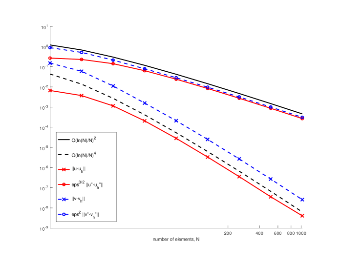
Figure 1: Shishkin meshes with $N\in[4,1024]$ elements, $\mathrm{eps}=\varepsilon=10^{-2}$.

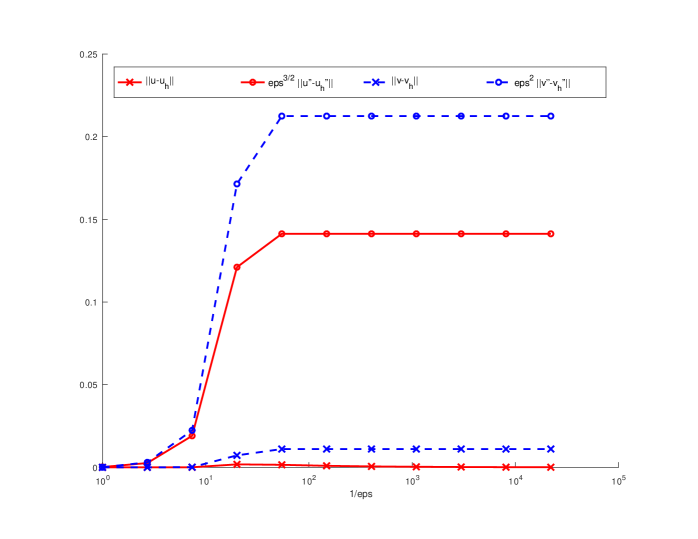
Figure 2: Shishkin mesh with $N=16$ elements, $\mathrm{eps}=\varepsilon\in[1,\mathrm{e}^{-10}]$.

References

[1]D. Chapelle and K.-J. Bathe, The finite element analysis of
shells—fundamentals, Computational Fluid and Solid Mechanics, Springer,
Heidelberg, second ed., 2011.
[2]P. R. B. Devloo, A. M. Farias, S. M. Gomes, and J. a. L. Gonçalves,
Application of a combined continuous-discontinuous Galerkin finite
element method for the solution of the Girkmann problem, Comput. Math.
Appl., 65 (2013), pp. 1786–1794.
[3]W. Flügge, Stresses in Shells, Springer-Verlag,
Berlin-Göttingen-Heidelberg, 1960.
Translation of Statik und Dynamik der Schalen, Springer, 1934.
[4]T.-L. Francis, V. A. Pulmano, and D. Thambiratnam, Bef analogy for