Constraints on peculiar velocity distribution of binary black holes using gravitational waves with GWTC-3

Abstract

The peculiar velocity encodes rich information about the formation, dynamics, evolution, and merging history of binary black holes. In this work, we employ a hierarchical Bayesian model to infer the peculiar velocity distribution of binary black holes for the first time using GWTC-3 by assuming a Maxwell-Boltzmann distribution for the peculiar velocities. The constraint on the peculiar velocity distribution parameter is rather weak and uninformative with the current GWTC-3 data release. However, the measurement of the peculiar velocity distribution can be significantly improved with the next-generation ground-based gravitational wave detectors. For instance, the uncertainty on the peculiar velocity distribution parameter will be measured within $\sim$ 10% with $10^{3}$ golden binary black hole events for the Einstein Telescope. We, therefore, conclude that our statistical approach provides a robust inference for the peculiar velocity distribution.

1 Introduction

The peculiar velocities are so sensitive to the matter distribution on large scales that we can use them as a useful cosmological probe and to test the link between gravity and matter [1]. General relativity predicts that gravitational waves (GWs) carry away linear momentum from binary systems, shifting the center of mass with a peculiar velocity [2, 3]. The non-zero radial component of the peculiar velocity for the compact binary coalescence system’s center of mass would produce a redshifted or blueshifted waveform. The peculiar velocity can be inferred using the recoil velocity of remnant black holes [4, 5] and a simple method given by Ref. [6]. Based on this method [7, 6, 8], the recoil velocity of the binary black hole (BBH) merger GW200129 [9] can be deduced to reach $\sim 1542$ $\mathrm{km}\,\mathrm{s^{-1}}$ [10]. Actually, the peculiar velocity evolves across the inspiral, merger, and ringdown phases and can, in principle, be inferred by observing the differential Doppler shift throughout the GW signal [7]. In this work, we study the average peculiar velocity of GW binaries instead of that at a specific time.

Recently, as advanced LIGO [11] and Virgo [12] improve their sensitivities and the fourth observing run starts, unprecedented opportunities arise to study the astrophysics of black holes, including directly measuring the peculiar velocities of GW sources. The direct measurement of the peculiar velocity, however, depends sensitively on the signal-to-noise ratio (SNR) of an event, as the recoil velocity can only be measured when the SNR is sufficiently high and by using a waveform calculated by numerical relativity surrogate models [13, 14, 15, 16]. Unfortunately, BBH events with large SNR are rare, and in GWTC-3 only three BBH events have an SNR $>20$, including GW200129 [9]. How to estimate the peculiar velocity of the majority of BBH events, which usually have low SNRs, remains an interesting problem.

As demonstrated in Ref. [17], peculiar velocity is an important input parameter in constraining the Hubble constant, $H_{0}$. Hence, one can constrain the peculiar velocity for a given cosmological model, providing an alternative method to infer the average peculiar velocity of BBHs. For a flat $\Lambda$CDM model with fixed cosmological parameters, the peculiar velocity encodes in the correlation between the redshifted mass and the luminosity distance distributions of black holes, which have no electromagnetic counterparts or host galaxy. Indeed, Ref. [1] has shown the relationship between the peculiar velocity and the resultant Doppler shift. For the BBH events detected by current GW observatories, due to the significant uncertainties in the parameter estimations, the reuslts of constraints on peculiar velocity distribution may not be ideal. However, in the era of third-generation ground-based detectors, such as the Einstein Telescope (ET) [18] and Cosmic Explorer (CE) [19], a significant improvement in BBH sample size and parameter estimation accuracy is expected. It will help enhance the result of peculiar velocity parameter inference because the ET/CE detector will be able to detect BBH mergers throughout the Universe, yielding $\sim 10^{4}-10^{7}$ discoveries per year [20, 21].

In this work, we simultaneously infer the peculiar velocity distribution and BBH population properties utilizing GWTC-3 and mock data from ET. This paper is organized as follows. In Section 2, we describe our model of BBH mass distribution. In Section 3, we introduce the redshift caused by the peculiar velocity of BBHs. Section 4 reviews the Bayesian hierarchical inference method used for analysis, while Section 5 shows the constraints on the peculiar velocity distribution. Finally, we summarize and discuss our results in Section 6. In addition, we show full posteriors using BBH events from GWTC-3 in Appendix A. Throughout this work, we have set the speed of light to unity, namely $c=1$.

2 BBH mass distribution

In this work, we introduce a method for jointly constraining peculiar velocity and source population properties of BBHs, without resorting to host galaxy information [22]. We use a phenomenological mass model, POWER LAW + PEAK, in the source frame for BBHs [23, 24], that is preferred by GWTC-3 [24]. The probability distribution of primary black hole mass is $\pi(m_{1})=\pi(m_{1}|\alpha,m_{\rm{min}},m_{\rm{max}},\lambda_{g},\mu_{g},\sigma_{g},\delta_{m})$, namely

$$\pi(m_{1})=\left[(1-\lambda_{g})\mathcal{P}(m_{1}|m_{\min},m_{\max},-\alpha)+\lambda_{g}\mathcal{G}(m_{1}|\mu_{{g}},\sigma_{{g}})\right]S(m_{1}|m_{\min},\delta_{m}),$$ (2.1)

where the truncated power law $\mathcal{P}(m|m_{\min},m_{\max},\alpha)$ with spectral index $\alpha$, lower cut-off $m_{\rm{min}}$ and upper cut-off $m_{\rm{max}}$ is described as,

$$\mathcal{P}(m|m_{\min},m_{\max},\alpha)=\begin{cases}m^{\alpha}&(m_{\min}\leqslant m\leqslant m_{\max}),\\ 0&\text{Otherwise}.\end{cases}$$ (2.2)

Meanwhile, the Gaussian component with mean $\mu_{g}$ and standard deviation $\sigma_{g}$ is given by

$$\mathcal{G}(m|\mu_{g},\sigma_{g})=\frac{1}{\sigma_{g}\sqrt{2\pi}}\exp\left[-\frac{(m-\mu_{g})^{2}}{2\sigma_{g}^{2}}\right].$$ (2.3)

The ratio of truncated power law and Gaussian component is $\lambda_{g}$. And the smoothing function, which rises from 0 to 1 over interval $(m_{\min},m_{\min}+\delta_{m})$ [23], is written as

$$S(m|m_{\min},\delta_{m})=\begin{cases}0&(m<m_{\min}),\\ {\left[f(m-m_{\min},\delta_{m})+1\right]^{-1}}&(m_{\min}\leq m<m_{\min}+\delta_{m}),\\ 1&(m\geq m_{\min}+\delta_{m}),\end{cases}$$ (2.4)

with

$$f(m^{\prime},\delta_{m})=\exp(\frac{\delta_{m}}{m^{\prime}}+\frac{\delta_{m}}{m^{\prime}-\delta_{m}}).$$ (2.5)

The secondary black hole mass distribution $\pi(m_{2})=\pi(m_{2}|m_{1},m_{\rm{\min}},\beta,\delta_{m})$, given the primary black hole mass $m_{1}$, is constructed by a truncated power-law with index $\beta$ between a minimum mass $m_{\rm{min}}$ and a maximum mass $m_{1}$, and a smoothing function $S(m_{2}|\delta_{m},m_{\min})$,

$$\pi(m_{2})=\mathcal{P}(m_{2}|m_{\min},m_{1},\beta)S(m_{2}|m_{\min},\delta_{m}).$$ (2.6)

Based on the above discussion, the source-frame mass distribution for the BBH population is

$$\pi(m_{1},m_{2}|\Phi_{m})=\pi(m_{1}|\alpha,m_{\min},m_{\max},\lambda_{g},\mu_{g},\sigma_{g},\delta_{m})\,\pi(m_{2}|m_{1},m_{\rm{\min}},\beta,\delta_{m}),$$ (2.7)

where $\Phi_{m}=\{\alpha,\beta,m_{\min},m_{\max},\lambda_{g},\mu_{g},\sigma_{g},\delta_{m}\}$ are the parameters that describe the BBHs mass distribution for POWER LAW + PEAK model.

3 Redshift induced by peculiar velocity

The mass and luminosity distance of GW events contain redshift information. The GW observatories detect redshifted black hole masses $m^{\rm{det}}_{i}$ and luminosity distance $D_{L}$ correlate with source-frame masses $m_{i}$ and redshift by

$$m_{i}=\frac{m_{i}^{\text{det}}}{1+z}.$$ (3.1)

We infer the redshift of GW events and use the spectrum siren method by tracking the mass spectrum in different luminosity distance bins for studying cosmic expansion and peculiar velocity of black holes.

In this work, we assume a flat Friedmann-Robertson-Walker Universe and a $\Lambda$CDM model by fixing cosmological parameters since we are interested in peculiar velocities. The Hubble rate at redshift $z$ is

$$H(z)=H_{0}E(z),$$ (3.2)

where $H_{0}$ is the Hubble constant, and

$$E(z)=\sqrt{{\Omega_{\mathrm{m}}}(1+z)^{3}+{\Omega_{\Lambda}}}.$$ (3.3)

The $\Omega_{m}$ and $\Omega_{\Lambda}$ represent the matter density and the dark energy density, respectively. In this work, we use the best-fit values of cosmological parameters from Planck 2018 [25], where $H_{0}=67.4\,\mathrm{km}\,\mathrm{s}^{-1}\,\mathrm{Mpc}^{-1}$, ${\Omega_{\mathrm{m}}}=0.315$, and ${\Omega_{\Lambda}}=1-{\Omega_{\mathrm{m}}}$. Given luminosity distance $D_{L}$ by GW observation, one can then calculate the redshift caused by cosmic expansion as

$$D_{L}=\frac{(1+z)}{H_{0}}\int_{0}^{z}\frac{dz^{\prime}}{E(z^{\prime})},$$ (3.4)

without considering the peculiar velocities of GW sources.

However, if the object has a peculiar velocity, an observer sees a dipole in the cosmic microwave background, and the object acquires an additional peculiar redshift component $z_{p}$. Note that the peculiar velocity is the sum of the projections of the peculiar velocities of two objects in binary systems along the line of sight from the observer and sources, i.e., the radial velocity component. The redshift of the GW sources with non-zero peculiar velocities can be described as,

$$1+z=(1+z_{cos})(1+z_{p}),$$ (3.5)

where the $z_{cos}$ is the redshift caused by Hubble flow, i.e., recession velocity, which can be calculated by Eq. (3.4), and $z_{p}$ is the redshift caused by peculiar velocities of GW sources. In Ref. [1], the relationship between $z_{p}$ and peculiar velocity $v_{p}$ is

$$1+z_{p}=\sqrt{\frac{1+v_{p}}{1-v_{p}}}.$$ (3.6)

When $v_{p}$ is much slower than the speed of light ($v_{p}\ll 1$), Eq. (3.6) can be approximated by $1+z_{p}\approx 1+v_{p}$. In this work, we simply assume the peculiar velocities follow a Maxwell-Boltzmann distribution as [26]

$$\pi(v_{p}|v_{0})\propto v_{p}^{2}\exp(-v_{p}^{2}/v_{0}^{2}),$$ (3.7)

where $v_{p}$ is the peculiar velocity of each BBH event, and $v_{0}$ is the most probable velocity of all BBH events. We set $v_{0}$ as a free parameter.

4 Hierarchical Bayesian inference

In this section, we introduce hierarchical Bayesian inference to estimate posterior distributions of parameters that describe the motion and the source population properties of BBHs. We use a cosmic star formation rate (SFR) model from [27] to describe the evolution of BBH binary merger rate since the black hole formation rate might track the SFR. The component $\psi(z|\gamma,k,z_{p})$ indicating the relation between BBH redshift and the merger rate is [27, 24]

$$\psi(z|\gamma,k,z_{\mathrm{pk}})=\left[1+(1+z_{\mathrm{pk}})^{-\gamma-k}\right]\frac{(1+z)^{\gamma}}{1+\left[(1+z)/(1+z_{\mathrm{pk}})\right]^{\gamma+k}},$$ (4.1)

with a peak at $z_{\rm{pk}}$, where $\gamma$ and $\kappa$ are the power-law indexes at low redshift and high redshift interval, respectively. Then the merger rate in the detector frame can be written as [28],

$$\mathcal{R}(z)=R_{0}\pi(z|\gamma,\kappa,z_{\rm{pk}}),$$ (4.2)

with

$$\pi(z|\gamma,\kappa,z_{\rm{pk}})=C\frac{1}{1+z}\frac{dV_{\mathrm{c}}}{dz}\psi(z|\gamma,k,z_{\mathrm{pk}}).$$ (4.3)

Eq. (4.2) gives the merger rate as a function of redshift. $R_{0}$ is the local merger rate, which is the integral of Eq. (4.2) over other observed parameters given at $z=0$. In the redshift prior function Eq. (4.3), $C$ is the normalisation factor, and $dV_{\mathrm{c}}/dz$ is the differential comoving volume. In order to convert the clock from the source frame to the detector frame, we multiply the factor ${1}/{(1+z)}$ by the redshift prior.

We have introduced the source mas and peculiar velocity distribution in Section 2 and Section 3. The complete characterization of the population models is the product of redshift, masss, and peculiar velocity prior, written as

$$p_{\text{pop}}(\theta|\Phi_{m},\gamma,\kappa,z_{\rm{pk}},v_{0})=C\frac{1}{1+z}\frac{dV_{\mathrm{c}}}{dz}\psi(z|\gamma,k,z_{p})\pi(m_{1},m_{2}|\Phi_{m})\pi(v_{p}|v_{0}),$$ (4.4)

where $\Phi_{m}=\{\alpha,\beta,m_{\min},m_{\max},\lambda_{g},\mu_{g},\sigma_{g},\delta_{m}\}$ is the POWER LAW + PEAK mass population parameters not related to cosmology and peculiar velocity, and $\theta=\{m_{1},m_{2},z,v_{p}\}$ are the intrinsic GW parameters. All parameters introduced above are shown in Table 1.

We are concerned with the distribution of BBH source parameters $\theta$ conditional upon the hyperparameters $(\Phi_{m},\gamma,\kappa,z_{\rm{pk}},v_{0})$, i.e. conditional prior $p_{\text{pop }}(\theta|\Phi_{m},\gamma,\kappa,z_{\rm{pk}},v_{0})$, by analysing $N_{\mathrm{obs}}$ GW data $\textbf{h}=\{h_{1},h_{2},\cdots,h_{{N_{\rm{obs}}}}\}$. Accordingly, the hyper-likelihood $\mathcal{L}(\mathbf{h}|\Phi_{m},\gamma,\kappa,z_{\rm{pk}},v_{0},R_{0})$ related to the single-event likelihood $\mathcal{L}(h_{i}|\theta)$ for the $i$-th event can be written as [29, 30, 31, 32, 33, 34, 35]

$$\mathcal{L}(\mathbf{h}|\Phi_{m},\gamma,\kappa,z_{\rm{pk}},v_{0},R_{0}) \propto R_{0}^{N_{\text{obs}}}e^{-R_{0}\xi(\Phi_{m},\gamma,\kappa,z_{\rm{pk}},v_{0})}$$ (4.5)

$$\times\prod_{i=1}^{N_{\text{obs}}}\int\mathcal{L}(h_{i}|\theta)p_{\text{pop}}(\theta|\Phi_{m},\gamma,\kappa,z_{\rm{pk}},v_{0})d\theta,$$

where $\xi(\Phi_{m},\gamma,\kappa,z_{\rm{pk}},v_{0})$ is the detection fraction that quantifies selection biases for a population based on hyperparameters $(\Phi_{m},\gamma,\kappa,z_{\rm{pk}},v_{0})$, described as

$$\xi(\Phi_{m},\gamma,\kappa,z_{\rm{pk}},v_{0})=\int P_{\mathrm{det}}(\theta)\,p_{\mathrm{pop}}(\theta|\Phi_{m},\gamma,\kappa,z_{\rm{pk}},v_{0})d\theta.$$ (4.6)

The detection probability based on the source parameters $\theta$ is $P_{\text{det}}(\theta)$, which is related to the simulated signals.

In this work, the simulated injections in [36] are used to compute the detection fraction $\xi(\Phi_{m},\gamma,\kappa,z_{\rm{pk}},v_{0})$. We utilise a Monte Carlo integral over found injections [37] to simplify Eq. (4.6) as

$$\xi(\Phi_{m},\gamma,\kappa,z_{\rm{pk}},v_{0})\approx\frac{1}{N_{\mathrm{inj}}}\sum_{j=1}^{N_{\text{found }}}\frac{p_{\mathrm{pop}}(\theta_{j}|\Phi_{m},\gamma,\kappa,z_{\rm{pk}},v_{0})}{p_{\mathrm{draw}}(\theta_{j})}.$$ (4.7)

In practice, we calculate the sum of the conditional prior divided by $p_{\mathrm{draw}}$ for each event instead of the integral. $p_{\text{draw }}$ is the regular prior distribution from which the injections are drawn, where $j$ indicates the $j$-th detected event. We employ the package, ICAROGW [38] including the BBH population distribution Eq. (4.4), to estimate the likelihood function Eq. (4.5), and then utilise dynesty [39] sampler in Bilby package [40, 41] to estimate the hyperparameters.

Parameter Description Prior Peculiar velocity distribution $v_{0}$ The most probable peculiar velocity. ${\rm{log}}{\mathcal{U}}(-5,-2)$ Merger rate evolution $R_{0}$ local merger rate of BBHs in $\mathrm{Gpc}^{-3}\mathrm{yr}^{-1}$. ${\mathcal{U}}(0,200)$ $\gamma$ Power-law index for the rate evolution before the point $z_{\mathrm{pk}}$. ${\mathcal{U}}(0,12)$ $\kappa$ Power-law index for the rate evolution after the point $z_{\mathrm{pk}}$. ${\mathcal{U}}(0,6)$ $z_{\mathrm{pk}}$ Redshift turning point between the powerlaw regimes with $\gamma$ and $\kappa$. ${\mathcal{U}}(0,4)$ POWER LAW + PEAK mass function $\alpha$ Spectral index for the power-law of the primary mass distribution. ${\mathcal{U}}(1.5,12)$ $\beta$ Spectral index for the power-law of the mass ratio distribution. ${\mathcal{U}}(-4,12)$ $m_{\min}\,[M_{\odot}]$ Minimum mass of the primary mass distribution. ${\mathcal{U}}(2,10)$ $m_{\max}\,[M_{\odot}]$ Maximum mass of the primary mass distribution. ${\mathcal{U}}(50,200)$ $\lambda_{g}$ Fraction of the model in the Gaussian component. ${\mathcal{U}}(0,1)$ $\mu_{g}\,[M_{\odot}]$ Mean of the Gaussian component in the primary mass distribution. ${\mathcal{U}}(20,50)$ $\sigma_{g}\,[M_{\odot}]$ Width of the Gaussian component in the primary mass distribution. ${\mathcal{U}}(0.4,10)$ $\delta_{m}\,[M_{\odot}]$ Range of mass tapering at the lower end of the mass distribution. ${\mathcal{U}}(0,10)$

Table 1: Parameters and their prior distributions used in the Bayesian parameter estimations. Note that $z_{p}$ and $z_{\rm{pk}}$ indicate the redshift caused by peculiar velocity and the redshift turning point of the merger rate evolution, respectively.

5 Results

In this section, we show results of hyperparameter estimation using the BBHs from GWTC-3, and the simulated BBH population expected to be detected by third-generation detectors such as ET.

5.1 GWTC-3

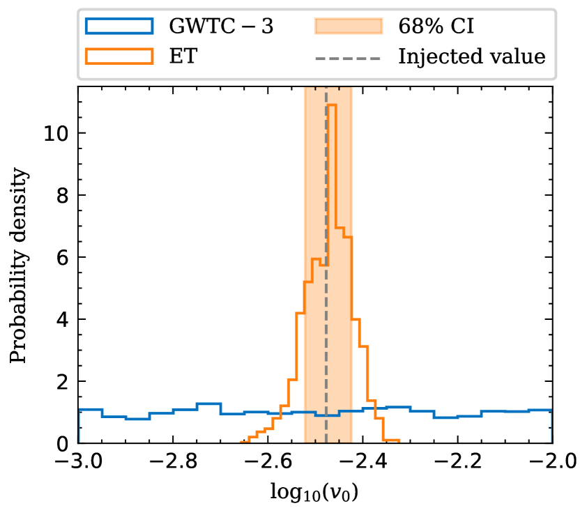
Figure 1: The one-dimensional marginal posterior distribution for $v_{0}$. The grey dash line is the injected value ${\rm{log}_{10}}(v_{0})=-2.48$ (corresponding to $v_{0}=3.33\times 10^{-3}$) for simulated events of ET. The blue solid and orange solid lines represent the posterior of $v_{0}$ derived from GWTC-3, and ET, respectively. The orange shaded area indicates the 68% credible interval, namely 1$\sigma$ region.

Similar to Refs. [24, 42], we use 42 BBH events with $\mathrm{SNR}>11$ and inverse false alarm rate higher than four years, excluding two BNS events [43, 44], two NSBH events [45] and one asymmetric mass binary GW190814 [46], from GWTC–3. We use combined posterior samples estimated by the IMRPhenom [47, 48] and SEOBNR [49, 50] waveform families. Based on the parameters estimation of these BBH sources, we perform data collection for the distribution of detector-frame masses and luminosity distance. Unlike the works interested in cosmological parameters estimation [51, 17, 24, 52, 53, 54], we are primarily concerned with peculiar velocity parameter of the BBH population. Based on the relationship between peculiar velocity and redshift, we employ Eqs. (3.4)-(3.6) to calculate peculiar velocity given the Hubble constant $H_{0}$ and matter density ${\Omega_{\mathrm{m}}}$ [25]. We show all parameters and their prior interval utilised for Bayesian parameter estimations in Table 1. Generally, these parameters can be divided into four categories: peculiar velocity distribution, merger rate evolution, POWER LAW + PEAK mass function, and cosmology.

We show extra details on the joint estimation of full posteriors in Figure 2 in Appendix A, including the peculiar velocity distribution parameter, merger rate evolution parameters, and mass function parameters using BBHs. For these corner plots of hyperparameters, most of the one-dimensional posterior for mass function and merger rate evolution parameters have the characteristics of Gaussian-like distribution except the peculiar velocity distribution parameter $v_{0}$. Figure 1 shows the marginal posterior distributions for the peculiar velocity parameters $v_{0}$. For comparison, we pick up a portion of the one-dimensional marginal posterior distribution for $v_{0}$ in Figure 2 to present as the blue histogram in Figure 1. There is no difference between the prior and posterior distributions, and they are flat distributions at logarithmic scale. Therefore, the peculiar velocity distribution posterior calculated from GWTC-3 is uninformative, indicating the current BBH events detected by LIGO-Virgo-KAGRA can not constrain the peculiar velocity distribution.

5.2 ET mock data

The posteriors derived using GWTC-3 in this work, shown in Figure 2, are consistent with the result in Ref. [24, 55]. To generate mock data for ET, we set the injected values based on our posterior results for POWER LAW + PEAK mass model parameters $\alpha=3.8$, $\beta=0.8$, $m_{\max}=100\mathrm{M}_{\odot}$, $m_{\min}=5\mathrm{M}_{\odot}$, $\delta_{m}=4.8\mathrm{M}_{\odot}$, $\mu_{g}=33\mathrm{M}_{\odot}$, $\sigma_{g}=3.2\mathrm{M}_{\odot}$, and $\lambda_{g}=0.03$, for the rate evolution model parameters $\gamma=4.7$, $k=3$, and $z_{\rm{pk}}=2.3$, and for BBH merger rate parameter $R_{0}=17\,\mathrm{Gpc}^{-3}\,\mathrm{yr}^{-1}$ at $z=0$. For the median value of peculiar velocity distribution $v_{0}$, we take a possible $v_{0}=3.33\times 10^{-3}$ (corresponding to $1000\,\mathrm{km}\,\mathrm{s}^{-1}$) following Ref. [26, 9]. The third-generation detectors, such as ET, are expected to detect approximately $\sim$ $10^{4}$ golden events for BBHs per year with $\leq 10\%$ error on luminosity distance and $\leq 0.02\%$ error on masses [56]. We conservatively simulate $10^{3}$ golden BBH events with $5\%$ error on luminosity distance and $0.02\%$ error on masses. To speed up the calculation, we generate 1000 posterior samples for individual events. Subsequently, we take these posterior into Eq. (4.5) to obtain hyper-posterior for peculiar velocity distribution.

The one-dimensional marginal posterior distribution of $v_{0}$ using $10^{3}$ golden BBH events detected with ET is shown as the orange histograms in Figure 1. Where the grey dash line indicates the injection value for $v_{0}$, and uniform priors for $v_{0}$ is $[10,4000]\,{\rm{km\,s^{-1}}}$. The result of posterior of $v_{0}$ is $1018^{+112}_{-115}\,\,\rm{km\,s^{-1}}$, measured with a 1$\sigma$ precision of $\sim$ 10% .

6 Conclusion and discussion

GW provides a new method to study the peculiar velocity distribution of BBHs. In this paper, we investigate how the detector-frame black hole mass distribution, which encodes information about cosmic expansion and peculiar velocity, can be utilized to infer the peculiar velocity distribution parameter without direct redshift measurement. We assume a $\Lambda$CDM cosmological model for peculiar velocity distribution parameters inference using GWTC-3. Our result indicates that for the current BBH events from GWTC-3, the constraint on $v_{0}$ is weak and uninformative. The small BBH sample and the large inaccuracy of mass and luminosity distance might affect the result of the peculiar velocity distribution parameter inference. On the other hand, we find that a one-year conservatively simulated observation of ET ($10^{3}$ golden BBH events) will constrain the peculiar velocity distribution parameter to $\sim 10\%$, with our current knowledge of the black hole mass function, and the merger rate evolution. If we have deeper understanding of the above quantities, which is plausible in the third-generation gravitational-wave detectors, more precision of constraints on peculiar velocity distribution is likely.

In this work, we for the first time provide a framework that allows simultaneous inference of peculiar velocity distribution, the mass function, and merger rate evolution parameters for black hole samples without electromagnetic counterparts or galaxy catalogues. We expect favourable constraints on the peculiar velocity distribution of the BBH events with $\mathcal{O}$(thousands) of GW sources and more accurate measurement as detector sensitivity improves by ET in the coming years. The accurate peculiar velocity distribution can aid in comprehending the formation, dynamics, evolution, and merging history of black holes. In the future, with the increased BBH sample and improved detectors, our approach might provide a robust inference for the peculiar velocity distribution of black holes.

Appendix A Posterior distributions of all hyperparameters

This appendix shows the posteriors of all the peculiar velocity distribution and population parameters using BBH events in GWTC-3. The corner plots are generated utilizing the corner [58] package.

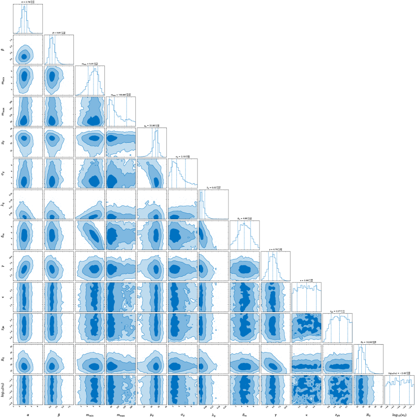
Figure 2: Posterior distributions of all the hyperparameters, including POWER LAW + PEAK mass function parameters ($\alpha,\beta,m_{\rm{min}},m_{\rm{max}},\mu_{g},\sigma_{g},\lambda_{g},\delta_{m}$), merger rate evolution parameters ($\gamma,\kappa,z_{\rm{pk}},R_{0}$), and the peculiar velocity distribution parameter $v_{0}$.

References

- [1] T.M. Davis and M.I. Scrimgeour, Deriving accurate peculiar velocities (even at high redshift), Monthly Notices of the Royal Astronomical Society 442 (2014) 1117 [1405.0105].
- [2] M.J. Fitchett, The influence of gravitational wave momentum losses on the centre of mass motion of a Newtonian binay system., Monthly Notices of the Royal Astronomical Society 203 (1983) 1049.
- [3] M. Ruiz, M. Alcubierre, D. Núñez and R. Takahashi, Multiple expansions for energy and momenta carried by gravitational waves, General Relativity and Gravitation 40 (2008) 1705 [0707.4654].
- [4] J.A. González, U. Sperhake, B. Brügmann, M. Hannam and S. Husa, Maximum Kick from Nonspinning Black-Hole Binary Inspiral, Physical Review Letters 98 (2007) 091101 [gr-qc/0610154].
- [5] C.O. Lousto and Y. Zlochower, Hangup Kicks: Still Larger Recoils by Partial Spin-Orbit Alignment of Black-Hole Binaries, Physical Review Letters 107 (2011) 231102 [1108.2009].
- [6] J. Calderón Bustillo, J.A. Clark, P. Laguna and D. Shoemaker, Tracking Black Hole Kicks from Gravitational-Wave Observations, Physical Review Letters 121 (2018) 191102 [1806.11160].
- [7] D. Gerosa and C.J. Moore, Black Hole Kicks as New Gravitational Wave Observables, Physical Review Letters 117 (2016) 011101 [1606.04226].
- [8] V. Varma, M. Isi and S. Biscoveanu, Extracting the Gravitational Recoil from Black Hole Merger Signals, Physical Review Letters 124 (2020) 101104 [2002.00296].
- [9] LIGO Scientific, VIRGO, KAGRA collaboration, GWTC-3: Compact Binary Coalescences Observed by LIGO and Virgo During the Second Part of the Third Observing Run, 2111.03606.
- [10] V. Varma, S. Biscoveanu, T. Islam, F.H. Shaik, C.-J. Haster, M. Isi et al., Evidence of Large Recoil Velocity from a Black Hole Merger Signal, Physical Review Letters 128 (2022) 191102 [2201.01302].
- [11] J. Aasi, B.P. Abbott, R. Abbott et al., Advanced LIGO, Classical and Quantum Gravity 32 (2015) 074001 [1411.4547].
- [12] F. Acernese, M. Agathos, K. Agatsuma et al., Advanced Virgo: a second-generation interferometric gravitational wave detector, Classical and Quantum Gravity 32 (2015) 024001 [1408.3978].
- [13] V. Varma, S.E. Field, M.A. Scheel, J. Blackman, D. Gerosa, L.C. Stein et al., Surrogate models for precessing binary black hole simulations with unequal masses, Physical Review Research 1 (2019) 033015 [1905.09300].
- [14] V. Varma, D. Gerosa, L.C. Stein, F. Hébert and H. Zhang, High-Accuracy Mass, Spin, and Recoil Predictions of Generic Black-Hole Merger Remnants, Physical Review Letters 122 (2019) 011101 [1809.09125].
- [15] V. Varma, S.E. Field, M.A. Scheel, J. Blackman, L.E. Kidder and H.P. Pfeiffer, Surrogate model of hybridized numerical relativity binary black hole waveforms, Physical Review D 99 (2019) 064045 [1812.07865].
- [16] J. Blackman, S.E. Field, M.A. Scheel, C.R. Galley, C.D. Ott, M. Boyle et al., Numerical relativity waveform surrogate model for generically precessing binary black hole mergers, Physical Review D 96 (2017) 024058 [1705.07089].
- [17] LIGO Scientific, Virgo, 1M2H, Dark Energy Camera GW-E, DES, DLT40, Las Cumbres Observatory, VINROUGE, MASTER collaboration, A gravitational-wave standard siren measurement of the Hubble constant, Nature 551 (2017) 85 [1710.05835].
- [18] M. Punturo, M. Abernathy, F. Acernese et al., The Einstein Telescope: a third-generation gravitational wave observatory, Classical and Quantum Gravity 27 (2010) 194002.
- [19] B.P. Abbott, R. Abbott, T.D. Abbott et al., Exploring the sensitivity of next generation gravitational wave detectors, Classical and Quantum Gravity 34 (2017) 044001 [1607.08697].
- [20] B. Sathyaprakash, M. Abernathy, F. Acernese et al., Scientific Potential of Einstein Telescope, arXiv e-prints (2011) arXiv:1108.1423 [1108.1423].
- [21] Z.-C. Chen and Q.-G. Huang, Distinguishing Primordial Black Holes from Astrophysical Black Holes by Einstein Telescope and Cosmic Explorer, JCAP 08 (2020) 039 [1904.02396].
- [22] S. Mastrogiovanni, K. Leyde, C. Karathanasis, E. Chassande-Mottin, D.A. Steer, J. Gair et al., On the importance of source population models for gravitational-wave cosmology, Physical Review D 104 (2021) 062009 [2103.14663].
- [23] R. Abbott, T.D. Abbott, S. Abraham and et al., Population Properties of Compact Objects from the Second LIGO-Virgo Gravitational-Wave Transient Catalog, The Astrophysical Journal Letters 913 (2021) L7 [2010.14533].
- [24] LIGO Scientific, VIRGO, KAGRA collaboration, Constraints on the cosmic expansion history from GWTC-3, 2111.03604.
- [25] Planck collaboration, Planck 2018 results. VI. Cosmological parameters, Astron. Astrophys. 641 (2020) A6 [1807.06209].
- [26] S. Bird, I. Cholis, J.B. Muñoz, Y. Ali-Haïmoud, M. Kamionkowski, E.D. Kovetz et al., Did LIGO detect dark matter?, Phys. Rev. Lett. 116 (2016) 201301 [1603.00464].
- [27] P. Madau and M. Dickinson, Cosmic Star-Formation History, Annual Review of Astronomy and Astrophysics 52 (2014) 415 [1403.0007].
- [28] T. Callister, M. Fishbach, D.E. Holz and W.M. Farr, Shouts and Murmurs: Combining Individual Gravitational-wave Sources with the Stochastic Background to Measure the History of Binary Black Hole Mergers, The Astrophysical Journal Letters 896 (2020) L32 [2003.12152].
- [29] T.J. Loredo, Accounting for source uncertainties in analyses of astronomical survey data, AIP Conf. Proc. 735 (2004) 195 [astro-ph/0409387].
- [30] E. Thrane and C. Talbot, An introduction to Bayesian inference in gravitational-wave astronomy: parameter estimation, model selection, and hierarchical models, Publ. Astron. Soc. Austral. 36 (2019) e010 [1809.02293].
- [31] I. Mandel, W.M. Farr and J.R. Gair, Extracting distribution parameters from multiple uncertain observations with selection biases, Mon. Not. Roy. Astron. Soc. 486 (2019) 1086 [1809.02063].
- [32] Z.-C. Chen, F. Huang and Q.-G. Huang, Stochastic Gravitational-wave Background from Binary Black Holes and Binary Neutron Stars and Implications for LISA, Astrophys. J. 871 (2019) 97 [1809.10360].
- [33] Z.-C. Chen, C. Yuan and Q.-G. Huang, Confronting the primordial black hole scenario with the gravitational-wave events detected by LIGO-Virgo, Phys. Lett. B 829 (2022) 137040 [2108.11740].
- [34] L. Liu, Z.-Q. You, Y. Wu and Z.-C. Chen, Constraining the merger history of primordial-black-hole binaries from GWTC-3, Phys. Rev. D 107 (2023) 063035 [2210.16094].
- [35] L.-M. Zheng, Z. Li, Z.-C. Chen, H. Zhou and Z.-H. Zhu, Towards a reliable reconstruction of the power spectrum of primordial curvature perturbation on small scales from GWTC-3, Phys. Lett. B 838 (2023) 137720 [2212.05516].
- [36] L.S. Collaboration, V. Collaboration and K. Collaboration, GWTC-3: Compact Binary Coalescences Observed by LIGO and Virgo During the Second Part of the Third Observing Run — O3 search sensitivity estimates, .
- [37] LIGO Scientific, VIRGO, KAGRA collaboration, The population of merging compact binaries inferred using gravitational waves through GWTC-3, 2111.03634.
- [38] S. Mastrogiovanni, K. Leyde, C. Karathanasis, E. Chassande-Mottin, D.A. Steer, J. Gair et al., On the importance of source population models for gravitational-wave cosmology, Phys. Rev. D 104 (2021) 062009 [2103.14663].
- [39] J.S. Speagle, dynesty: a dynamic nested sampling package for estimating Bayesian posteriors and evidences, Mon. Not. Roy. Astron. Soc. 493 (2020) 3132 [1904.02180].
- [40] G. Ashton et al., BILBY: A user-friendly Bayesian inference library for gravitational-wave astronomy, Astrophys. J. Suppl. 241 (2019) 27 [1811.02042].
- [41] I.M. Romero-Shaw et al., Bayesian inference for compact binary coalescences with bilby: validation and application to the first LIGO–Virgo gravitational-wave transient catalogue, Mon. Not. Roy. Astron. Soc. 499 (2020) 3295 [2006.00714].
- [42] Z.-C. Chen, S.-S. Du, Q.-G. Huang and Z.-Q. You, Constraints on primordial-black-hole population and cosmic expansion history from GWTC-3, JCAP 03 (2023) 024 [2205.11278].
- [43] B.P. Abbott, R. Abbott, T.D. Abbott and et al., GW170817: Observation of Gravitational Waves from a Binary Neutron Star Inspiral, Physical Review Letters 119 (2017) 161101 [1710.05832].
- [44] B.P. Abbott, R. Abbott, T.D. Abbott and et al., GW190425: Observation of a Compact Binary Coalescence with Total Mass 3.4 M⊙, The Astrophysical Journal Letters 892 (2020) L3 [2001.01761].
- [45] R. Abbott, T.D. Abbott, S. Abraham, F. Acernese and et al., Observation of Gravitational Waves from Two Neutron Star-Black Hole Coalescences, The Astrophysical Journal Letters 915 (2021) L5 [2106.15163].
- [46] R. Abbott, T.D. Abbott, S. Abraham, F. Acernese and et al., GW190814: Gravitational Waves from the Coalescence of a 23 Solar Mass Black Hole with a 2.6 Solar Mass Compact Object, The Astrophysical Journal Letters 896 (2020) L44 [2006.12611].
- [47] J.E. Thompson, E. Fauchon-Jones, S. Khan, E. Nitoglia, F. Pannarale, T. Dietrich et al., Modeling the gravitational wave signature of neutron star black hole coalescences, Phys. Rev. D 101 (2020) 124059 [2002.08383].
- [48] G. Pratten et al., Computationally efficient models for the dominant and subdominant harmonic modes of precessing binary black holes, Phys. Rev. D 103 (2021) 104056 [2004.06503].
- [49] S. Ossokine et al., Multipolar Effective-One-Body Waveforms for Precessing Binary Black Holes: Construction and Validation, Phys. Rev. D 102 (2020) 044055 [2004.09442].
- [50] A. Matas et al., Aligned-spin neutron-star–black-hole waveform model based on the effective-one-body approach and numerical-relativity simulations, Phys. Rev. D 102 (2020) 043023 [2004.10001].
- [51] W.M. Farr, M. Fishbach, J. Ye and D.E. Holz, A Future Percent-level Measurement of the Hubble Expansion at Redshift 0.8 with Advanced LIGO, The Astrophysical Journal Letters 883 (2019) L42 [1908.09084].
- [52] J.M. Ezquiaga and D.E. Holz, Spectral Sirens: Cosmology from the Full Mass Distribution of Compact Binaries, Physical Review Letters 129 (2022) 061102 [2202.08240].
- [53] Z.-Q. You, X.-J. Zhu, G. Ashton, E. Thrane and Z.-H. Zhu, Standard-siren cosmology using gravitational waves from binary black holes, Astrophys. J. 908 (2021) 215 [2004.00036].
- [54] Z.-C. Chen, S.-S. Du, Q.-G. Huang and Z.-Q. You, Constraints on primordial-black-hole population and cosmic expansion history from GWTC-3, Journal of Cosmology and Astroparticle Physics 2023 (2023) 024 [2205.11278].
- [55] R. Abbott, T.D. Abbott, F. Acernese and et al., Population of Merging Compact Binaries Inferred Using Gravitational Waves through GWTC-3, Physical Review X 13 (2023) 011048.
- [56] M. Branchesi, M. Maggiore, D. Alonso, C. Badger, B. Banerjee, F. Beirnaert et al., Science with the Einstein Telescope: a comparison of different designs, arXiv e-prints (2023) arXiv:2303.15923 [2303.15923].
- [57] LIGO Scientific Collaboration and Virgo collaboration, Gravitational Wave Open Science Center, https://www.gw-openscience.org .
- [58] D. Foreman-Mackey, corner.py: Scatterplot matrices in python, The Journal of Open Source Software 1 (2016) 24.