On the use of the Gram matrix for multivariate functional principal components analysis

Abstract

Dimension reduction is crucial in functional data analysis (FDA). The key tool to reduce the dimension of the data is functional principal component analysis. Existing approaches for functional principal component analysis usually involve the diagonalization of the covariance operator. With the increasing size and complexity of functional datasets, estimating the covariance operator has become more challenging. Therefore, there is a growing need for efficient methodologies to estimate the eigencomponents. Using the duality of the space of observations and the space of functional features, we propose to use the inner-product between the curves to estimate the eigenelements of multivariate and multidimensional functional datasets. The relationship between the eigenelements of the covariance operator and those of the inner-product matrix is established. We explore the application of these methodologies in several FDA settings and provide general guidance on their usability.

Keywords— Dimension Reduction; Functional Data Analysis; Functional Principal Components; Multivariate Functional Data

1 Introduction

Functional data analysis (FDA) is a statistical methodology for analyzing data that can be characterized as functions. These functions could represent measurements taken over time or space, such as temperature readings over a yearly period or spatial patterns of disease occurrence. The goal of FDA is to extract meaningful information from these functions and to model their behavior. See, e.g., Ramsay and Silverman, (2005); Horvàth and Kokoszka, (2012); Wang et al., (2016); Kokoszka et al., (2017) for some references on FDA.

Functional principal component analysis (FPCA) is an extension of principal component analysis (PCA, a commonly used tool for dimension reduction in multivariate data) to functional data. FPCA was introduced by Karhunen, (1947) and Loève, (1945) and developed by Dauxois et al., (1982). Since then, FPCA has become a prevalent tool in FDA due to its ability to convert infinite-dimensional functional data into finite-dimensional vectors of random scores. These scores are a countable sequence of uncorrelated random variables that can be truncated to a finite vector in practical applications. By applying multivariate data analysis tools to these random scores, FPCA can achieve the goal of dimension reduction while assuming mild assumptions about the underlying stochastic process. FPCA is usually used as a preprocessing step to feed, e.g., regression and classification models. Recently, FPCA has been extended to multivariate functional data, which are data that consist of multiple functions that are observed simultaneously. This extension is referred to as multivariate functional principal component analysis (MFPCA). As for FPCA, a key benefit of MFPCA is that it allows one to identify and visualize the main sources of variation in the multivariate functional data. This can be useful in different applications, such as identifying patterns of movements in sport biomechanics (Warmenhoven et al.,, 2019), analyzing changes in brain activity in neuroscience (Song and Kim,, 2022), or comparing countries’ competitiveness in economics (Krzyśko et al.,, 2022).

In MFPCA, we seek to decompose the covariance structure of the multivariate functional data into a set of orthogonal basis functions, named the principal components, which capture the main sources of variation in the data. There are multiple approaches to estimate the principal components of a multivariate functional dataset. Ramsay and Silverman, (2005) combine the multivariate curves into one big curve and then perform a usual FPCA via an eigendecomposition of the covariance structure. This methodology can only be run for data that are defined on the same unidimensional domain, that exhibit similar amounts of variability and are measured in the same units. Jacques and Preda, (2014) propose to represent each feature of the multivariate function separately using a basis function expansion. This results in a different set of coefficients for each univariate curve. The eigendecomposition is then run on the matrix of stacked coefficients. To consider the normalization issue of Ramsay and Silverman, (2005), Jacques and Preda, (2014) and Chiou et al., (2014) propose to normalize the data by the standard deviation of the curves at each of the sampling points. Happ and Greven, (2018) extend the estimation of multivariate principal components to functional data defined on different dimensional domains. Their estimation procedure is based on carrying out FPCA on each univariate feature, and then using a weighted combination of the resulting principal components to obtain the multivariate eigencomponents. Finally, Berrendero et al., (2011) develop a different method to estimate the eigencomponents as they perform a principal components analysis for each sampling time point.

The key motivation of this paper is to investigate the duality between rows and columns of a data matrix to estimate the eigencomponents of a multivariate functional dataset. The duality between rows and columns of a data matrix is a fundamental concept in classical multivariate statistics (Escofier,, 1979; Saporta,, 1990). A data matrix typically represents a set of observations of multiple features, each row corresponds to an individual observation and each column corresponds to an individual feature. The duality between rows and columns refers to the fact that many statistical methodologies can be conducted either on the rows or the columns of the data matrix, and the results will be related to each other. For example, the principal components obtained from a PCA run on the rows of the data matrix are the same as the ones obtained from a PCA run on the columns of the matrix. The choice of method to use, based on criteria such as computational time or data storage needs, is thus left to the statistician. This concept has been widely studied in multivariate statistics (see, e.g., Pagès, (2014); Härdle and Simar, (2019)). In the context of functional data, this principle has received limited attention despite being mentioned in the seminal paper of FDA (Ramsay,, 1982). Ramsay and Silverman, (2005) briefly commented on it in a concluding remark of Chapter 8, while Kneip and Utikal, (2001) and Benko et al., (2009) utilized it to compute principal components for dense univariate functional data. Chen et al., (2017) also employ it to gain computational advantage when univariate functional data are sampled on a very dense grid. To the best of our knowledge, however, there is no available literature on its application to multivariate functional data that are observed on different dimensional domains. Our aim is therefore to investigate this duality for multivariate functional data observed on different dimensional domains and provide guidelines to statisticians on which method to use in different cases.

The remainder of the paper is organized as follows. In Section 2, we define multivariate functional data, with components that are observed on possibly different domains. In Section 3, we develop the duality between the observations’ space and the functional components’ space. The relationship between the eigencomponents of the covariance operator of the multivariate functional datasets and the eigencomponents of the inner-product matrix between the observations is derived in Section 4. Extensive simulations are given in Section 5. We also provide guidelines on which method to use with respect to different data characteristics. The paper concludes with a discussion and an outlook in Section 6.

2 Model

The structure of the data we consider, referred to as multivariate functional data, is similar to that presented in Happ and Greven, (2018). The data consist of independent trajectories of a vector-valued stochastic process $X=(X^{(1)},\dots,X^{(P)})^{\top}$, $P\geq 1$. (Here and in the following, for any matrix $A$, $A^{\top}$ denotes its transpose.) For each $1\leq p\leq P$, let $\mathcal{T}_{p}$ be a rectangle in some Euclidean space $\mathbb{R}^{d_{p}}$ with $d_{p}\geq 1$, e.g., $\mathcal{T}_{p}=[0,1]^{d_{p}}$. Each coordinate $X^{(p)}:\mathcal{T}_{p}\rightarrow\mathbb{R}$ is assumed to belong to $\mathcal{L}^{2}\left(\mathcal{T}_{p}\right)$, the Hilbert space of square-integrable real-valued functions defined on $\mathcal{T}_{p}$, having the usual inner product that we denote by $\left\langle\cdot,\cdot\right\rangle$, and $\left|\!\left|\cdot\right|\!\right|$ the associated norm. Thus $X$ is a stochastic process indexed by $\mathbf{t}=(t_{1},\ldots,t_{P})$ belonging to the $P-$fold Cartesian product $\mathcal{T}:=\mathcal{T}_{1}\times\cdots\times\mathcal{T}_{P}$ and taking values in the $P-$fold Cartesian product space $\mathcal{H}\coloneqq\mathcal{L}^{2}\left(\mathcal{T}_{1}\right)\times\dots\times\mathcal{L}^{2}\left(\mathcal{T}_{P}\right)$.

We consider the function $\langle\!\langle\cdot,\cdot\rangle\!\rangle:\mathcal{H}\times\mathcal{H}\rightarrow\mathbb{R}$,

$$\langle\!\langle f,g\rangle\!\rangle\coloneqq\sum_{p=1}^{P}\left\langle f^{(p)},g^{(p)}\right\rangle=\sum_{p=1}^{P}\int_{\mathcal{T}_{p}}f^{(p)}(t_{p})g^{(p)}(t_{p}){\rm d}t_{p},\quad f,g\in\mathcal{H}.$$ (1)

$\mathcal{H}$ is a Hilbert space with respect to the inner product $\langle\!\langle\cdot,\cdot\rangle\!\rangle$(Happ and Greven,, 2018). We denote by $\left|\!\left|\!\left|\cdot\right|\!\right|\!\right|$, the norm induced by $\langle\!\langle\cdot,\cdot\rangle\!\rangle$. Let $\mu:\mathcal{T}\rightarrow\mathcal{H}$ denote the mean function of the process $X$, $\mu(\mathbf{t})\coloneqq\mathbb{E}(X(\mathbf{t})),\,\mathbf{t}\in\mathcal{T}$. Let $C$ denote the $P\times P$ matrix-valued covariance function which, for $\mathbf{s},\mathbf{t}\in\mathcal{T}$, is defined as

$$C(\mathbf{s},\mathbf{t})\coloneqq\mathbb{E}\left(\{X(\mathbf{s})-\mu(\mathbf{s})\}\{X(\mathbf{t})-\mu(\mathbf{t})\}^{\top}\right),\quad\mathbf{s},\mathbf{t}\in\mathcal{T}.$$ (2)

More precisely, for $1\leq p,q\leq P$, the $(p,q)$th entry of the matrix $C(\mathbf{s},\mathbf{t})$ is the covariance function between the $p$th and the $q$th features of the process $X$:

$$C_{p,q}(s_{p},t_{q})\coloneqq\mathbb{E}\left(\{X^{(p)}(s_{p})-\mu^{(p)}(s_{p})\}\{X^{(q)}(t_{q})-\mu^{(q)}(t_{q})\}\right),\quad s_{p}\in\mathcal{T}_{p},t_{q}\in\mathcal{T}_{q}.$$ (3)

Let $\Gamma:\mathcal{H}\rightarrow\mathcal{H}$ denote the covariance operator of $X$, defined as an integral operator with kernel $C$. That is, for $f\in\mathcal{H}$ and $\mathbf{t}\in\mathcal{T}$, the $p$th feature of $\Gamma f(\mathbf{t})$ is given by

$$(\Gamma f)^{(p)}(t_{p})\coloneqq\langle\!\langle C_{p,\cdot}(t_{p},\cdot),f(\cdot)\rangle\!\rangle=\langle\!\langle C_{\cdot,p}(\cdot,t_{p}),f(\cdot)\rangle\!\rangle,\quad t_{p}\in\mathcal{T}_{p}.$$ (4)

Let us consider a set of $N$ curves $\mathcal{X}=\{X_{1},\ldots,X_{n},\ldots,X_{N}\}$ generated as a random sample of the $P$-dimensional stochastic process $X$ with continuous trajectories. Unless otherwise stated, the data are assumed to be observed without error. The data can be viewed as a table with $N$ rows and $P$ columns where each entry is a curve, potentially on a multidimensional domain (see Figure 1). Each row of this matrix represents an observation; while each column represents a functional feature. At the intersection of row $n$ and column $p$, we thus have $X_{n}^{(p)}$ which is the curve that concerns the (functional) feature $p$ for the individual $n$.

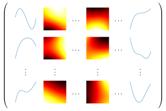
Figure 1: Functional data matrix, adapted from Berrendero et al., (2011).

For $n\in\{1,\dots,N\}$, each observation $n$ is attributed the weight $\pi_{n}$ such that $\sum_{n}\pi_{n}=1$, e.g., $\pi_{n}=1/N$. For a given $p\in\{1,\dots,P\}$, the mean curve of the $p$th feature along the $N$ observations is denoted by $\mu^{(p)}$. This quantity can be computed as

$$\mu^{(p)}(t_{p})=\sum_{n=1}^{N}\pi_{n}X_{n}^{(p)}(t_{p}),\quad t_{p}\in\mathcal{T}_{p},\quad p\in\{1,\dots,P\}.$$

The cross-covariance function of the $p$th and $q$th features along the $N$ observations can be computed as, for $p=1,\dots,P$ and $q=1,\dots,P$,

$$C_{p,q}(s_{p},t_{q})=\sum_{n=1}^{N}\pi_{n}X_{n}^{(p)}(s_{p})X_{n}^{(q)}(t_{q})-\mu^{(p)}(s_{p})\mu^{(q)}(t_{q}),\quad s_{p}\in\mathcal{T}_{p},\quad t_{q}\in\mathcal{T}_{q}.$$ (5)

For the set $\mathcal{X}$, the inner-product matrix, also called the Gram matrix, $\mathbf{M}$ is defined as a matrix of size $N\times N$ with entries

$$\mathbf{M}_{nn^{\prime}}=\sqrt{\pi_{n}\pi_{n^{\prime}}}\langle\!\langle X_{n}-\mu,X_{n^{\prime}}-\mu\rangle\!\rangle,\quad n,n^{\prime}=1,\dots,N.$$ (6)

This matrix is symmetric, positive definite, and interpretable as a proximity matrix, each entry being the distance between the weighted observations.

2.1 Basis decomposition

In many practical situations, functional data are noisy and only observed at specific time points. To extract the underlying functional features of the data, smoothing and interpolation techniques are commonly employed. These techniques involve approximating the true underlying function generating the data by a finite-dimensional set of basis functions. Assume that for each feature $p=1,\dots,P$, there exists a set of basis of functions $\Psi^{(p)}=\{\psi_{k}^{(p)}\}_{1\leq k\leq K_{p}}$ such that each feature of each curve $n=1,\dots,N$ can be expanded using the basis:

$$X_{n}^{(p)}(t_{p})=\sum_{k=1}^{K_{p}}c^{(p)}_{nk}\psi_{k}^{(p)}(t_{p}),\quad t_{p}\in\mathcal{T}_{p},$$ (7)

where $\{c^{(p)}_{nk}\}_{1\leq k\leq K_{p}}$ is a set of coefficients for feature $p$ of observation $n$. We denote by $\overline{c}_{k}^{(p)}=\sum_{n=1}^{N}\pi_{n}c^{(p)}_{nk}$ the mean coefficient of feature $p$ corresponding to the $k$th basis function. The $p$th feature of the mean function can be then expanded in the same basis as:

$$\mu^{(p)}(t_{p})=\sum_{k=1}^{K_{p}}\overline{c}_{k}^{(p)}\psi_{k}^{(p)}(t_{p}),\quad t_{p}\in\mathcal{T}_{p}.$$ (8)

Similarly, the covariance function of the $p$th and $q$th features is given by:

$$C_{p,q}(s_{p},t_{q})=\sum_{k=1}^{K_{p}}\sum_{l=1}^{K_{q}}\left(\sum_{n=1}^{N}\pi_{n}c^{(p)}_{nk}c^{(q)}_{nl}-\overline{c}_{k}^{(p)}\overline{c}_{l}^{(q)}\right)\psi_{k}^{(p)}(s_{p})\psi_{l}^{(q)}(t_{q}),\quad s_{p}\in\mathcal{T}_{p},\quad t_{q}\in\mathcal{T}_{q}.$$ (9)

These formulas can be written in matrix form as follows. For $\mathbf{t}\in\mathcal{T}$, we have that $X(\mathbf{t})=\mathbf{C}\Psi(\mathbf{t})$ where $X(\mathbf{t})$ is a $N\times P$ matrix with entries $X_{n}^{(p)}(t_{p}),\leavevmode\nobreak\ t_{p}\in\mathcal{T}_{p},\leavevmode\nobreak\ 1\leq p\leq P,\leavevmode\nobreak\ 1\leq n\leq N$,

$$\mathbf{C}=\begin{pmatrix}\mathbf{C}^{(1)}&\cdots&\mathbf{C}^{(P)}\\ \end{pmatrix},\quad\text{and}\quad\Psi(\mathbf{t})=\text{diag}\{\Psi^{(1)}(t_{1}),\dots,\Psi^{(P)}(t_{P})\},$$ (10)

where

$$\mathbf{C}^{(p)}=\begin{pmatrix}c^{(p)}_{11}&\cdots&c^{(p)}_{1K_{p}}\\ \vdots&\ddots&\vdots\\ c^{(p)}_{N1}&\cdots&c^{(p)}_{NK_{p}}\end{pmatrix}\\ \quad\text{and}\quad\Psi^{(p)}(t_{p})=\begin{pmatrix}\psi_{1}^{(p)}(t_{p})\\ \vdots\\ \psi_{K_{p}}^{(p)}(t_{p})\end{pmatrix}.$$ (11)

Using the basis expansion and denoting $\Pi^{\top}=(\pi_{1},\dots,\pi_{N})$, the mean and covariance functions are given by

$$\mu(\mathbf{t})=\Psi(\mathbf{t})^{\top}\mathbf{C}^{\top}\Pi\quad\text{and}\quad C(\mathbf{s},\mathbf{t})=\Psi(\mathbf{s})^{\top}\mathbf{C}^{\top}\left(\text{diag}\{\pi_{1},\dots,\pi_{N}\}-\Pi\Pi^{\top}\right)\mathbf{C}\Psi(\mathbf{t}).$$ (12)

Finally, we denote by $\mathbf{W}$ the matrix of inner products of the functions in the basis $\Psi$. The matrix $\mathbf{W}$ is a block-diagonal matrix such that $\mathbf{W}=\text{diag}\{\mathbf{W}^{(1)},\dots,\mathbf{W}^{(P)}\}$ where each entry is given by

$$\mathbf{W}_{k,l}^{(p)}=\left\langle\psi_{k}^{(p)},\psi_{l}^{(p)}\right\rangle,\quad 1\leq k,l\leq K_{p},\quad 1\leq p\leq P.$$ (13)

We remark that, if the basis $\Psi$ is an orthonormal basis, the matrix $\mathbf{W}$ is equal to the identity matrix of size $\sum_{p=1}^{P}K_{p}$. Using the expansion of the data into the basis of functions $\Psi$, the inner-product matrix $\mathbf{M}$ is written

$$\mathbf{M}=\text{diag}\{\sqrt{\pi_{1}},\dots,\sqrt{\pi_{N}}\}\left(\mathrm{I}_{\!N}-\mathbf{1}_{\!N}\Pi^{\top}\right)\mathbf{C}\mathbf{W}\mathbf{C}^{\top}\left(\mathrm{I}_{\!N}-\Pi\mathbf{1}_{\!N}^{\top}\right)\text{diag}\{\sqrt{\pi_{1}},\dots,\sqrt{\pi_{N}}\}$$ (14)

where $\mathrm{I}_{\!N}$ is the identity matrix of size $N$ and $\mathbf{1}_{\!N}$ is a vector of $1$ of length $N$.

3 On the geometry of multivariate functional data

3.1 Duality diagram

The distinction between the space of rows of a matrix as a sample from a population and the space of columns as the fixed variables on which the observations were measured has been explained in Holmes, (2008) and De la Cruz and Holmes, (2011) for multivariate data analysis. We propose to define a duality diagram in the context of multivariate functional data. Consider the data matrix defined by the set $\mathcal{X}$. We define an operator $L_{X}:\mathcal{H}\rightarrow\mathbb{R}^{N}$ by

$$L_{X}:f\mapsto\begin{pmatrix}\sqrt{\pi_{1}}\langle\!\langle X_{1}-\mu,f\rangle\!\rangle\\ \vdots\\ \sqrt{\pi_{N}}\langle\!\langle X_{N}-\mu,f\rangle\!\rangle\end{pmatrix}.$$ (15)

Using the linearity of the inner-product $\langle\!\langle\cdot,\cdot\rangle\!\rangle$ and vectors, the operator $L_{X}$ is linear. Define the operator $L^{\star}_{X}:\mathbb{R}^{N}\rightarrow\mathcal{H}$ as

$$L^{\star}_{X}:u\mapsto\begin{pmatrix}\sum_{n=1}^{N}\sqrt{\pi_{n}}u_{n}\{X_{n}^{(1)}(t_{1})-\mu^{(1)}(t_{1})\}\\ \vdots\\ \sum_{n=1}^{N}\sqrt{\pi_{n}}u_{n}\{X_{n}^{(P)}(t_{P})-\mu^{(P)}(t_{P})\}\end{pmatrix}.$$ (16)

Then $L^{\star}_{X}$ is the adjoint operator of the linear operator $L_{X}$ (see Appendix A for a proof). As an adjoint operator, $L^{\star}_{X}$ is a linear operator. The operator $\Gamma$ and the matrix $\mathbf{M}$ define geometries in $\mathcal{H}$ and $\mathbb{R}^{N}$, respectively, through

$$\langle\!\langle f,g\rangle\!\rangle_{\Gamma}=\langle\!\langle f,\Gamma g\rangle\!\rangle,\quad f,g\in\mathcal{H},\quad\text{and}\quad\left(u,v\right)_{\mathbf{M}}=u^{\top}\mathbf{M}v,\quad u,v\in\mathbb{R}^{N}.$$ (17)

We denote by $\left|\!\left|\!\left|\cdot\right|\!\right|\!\right|_{\Gamma}$ and $\left(\!\left(\cdot\right)\!\right)_{\mathbf{M}}$ their associated norms. Using the definition of adjoint operators $L_{X}$ and $L^{\star}_{X}$, we have that

$$\left(L_{X}(f),u\right)_{\mathbf{M}}=\langle\!\langle f,L^{\star}_{X}(u)\rangle\!\rangle_{\Gamma},\quad\text{for all}\quad f\in\mathcal{H},u\in\mathbb{R}^{N}.$$ (18)

These relationships can be expressed as a duality diagram, see Figure 2. The triplet $(X,\Gamma,\mathbf{M})$ defines a (multivariate) functional data analysis framework. One consequence of this transition between spaces is that the eigencomponents of $\mathcal{X}$ can be estimated equivalently using either the covariance operator $\Gamma$ or the Gram matrix $\mathbf{M}$. The relationship between the eigencomponents of $\Gamma$ and the eigencomponents of $\mathbf{M}$ are derived in Section 4.

Figure 2: Duality diagram between the spaces $\mathcal{H}$ and $\mathbb{R}^{N}$. The operator $L_{X}$ and its adjoint $L^{\star}_{X}$ are linear operators. The covariance operator $\Gamma$ and the matrix $\mathbf{M}$ define geometries in $\mathcal{H}$ and $\mathbb{R}^{N}$ respectively. The space $\mathcal{H}^{\star}$ (resp. $\mathbb{R}^{N\star}$) is the dual space of $\mathcal{H}$ (resp. $\mathbb{R}^{N}$).

Remark 1.

In general, in order to avoid confusion, inner-products and norms in function space, $\mathcal{H}$ or $\mathcal{L}^{2}\left(\mathcal{T}\right)$, will be refered with angle brackets, $\left\langle\cdot,\cdot\right\rangle$, while inner-products and norms in coordinate space, $\mathbb{R}^{N}$, will be refered with round brackets, $\left(\cdot,\cdot\right)$.

Remark 2.

We present here the duality diagram for the linear integral operator $\Gamma$ with kernel $C$. It is however possible to define duality diagrams for more general linear integral operators defined with a continuous symmetric positive definite function as kernel (see González and Muñoz, (2010) and Wong and Zhang, (2019) for discussions on possible integral operators to represent univariate functional data).

3.2 Cloud of individuals

Given an element $f\in\mathcal{H}$, let $\{f^{(p)}(t_{p}),\,t_{p}\in\mathcal{T}_{p},\,p=1,\dots,P\}$ be the features set of the element. We identify this set as the point $\mathrm{M}_{f}$ in the space $\mathcal{H}$. The space $\mathcal{H}$ is referred to as the observation space. The cloud of points that represents the set of observations $\mathcal{X}$ in $\mathcal{H}$ is denoted by $\mathcal{C}_{\!P}$. Let $\mathrm{G}_{\!\mu}$ be the centre of gravity of the cloud $\mathcal{C}_{\!P}$. In the space $\mathcal{H}$, its coordinates are given by $\{\mu^{(p)}(t_{p}),\,t_{p}\in\mathcal{T}_{p},\,p=1,\dots,P\}$. If the features are centered, the origin $\mathrm{O}_{\!\mathcal{H}}$ of the axes in $\mathcal{H}$ coincides with $\mathrm{G}_{\!\mu}$.

Figure 3: Left: Cloud of observations. Right: Projection of the points onto the elements of $\mathcal{H}$. The observation $f$ (resp. $g$) is identified by the point $\mathrm{M}_{f}$ (resp. $\mathrm{M}_{g}$) in the cloud $\mathcal{C}_{\!P}$. The point $\mathrm{G}_{\!\mu}$ is the center of gravity of $\mathcal{C}_{\!P}$ and the point $\mathrm{O}_{\!\mathcal{H}}$ is the origin of the space $\mathcal{H}$.

Let $f$ and $g$ be two elements in $\mathcal{H}$ and denote by $\mathrm{M}_{f}$ and $\mathrm{M}_{g}$ their associated points in $\mathcal{C}_{\!P}$ (see Figure 3). The most natural distance between these observations is based on the usual inner product in $\mathcal{H}$, $\langle\!\langle\cdot,\cdot\rangle\!\rangle$, and is defined as

$$d^{2}(\mathrm{M}_{f},\mathrm{M}_{g})=\left|\!\left|\!\left|f-g\right|\!\right|\!\right|^{2}=\sum_{p=1}^{P}\int_{\mathcal{T}_{p}}\left\{f^{(p)}(t_{p})-g^{(p)}(t_{p})\right\}^{2}{\rm d}t_{p}.$$ (19)

This distance measures how different the observations are, and thus gives one characterization of the shape of the cloud $\mathcal{C}_{\!P}$. Another description of this shape is to consider the distance between each observation and $\mathrm{G}_{\!\mu}$, the center of the cloud. Let $f$ be an element of $\mathcal{H}$, associated to the point $\mathrm{M}_{f}$, and $\mu$ the element of $\mathcal{H}$ related to $\mathrm{G}_{\!\mu}$, the distance between $f$ and $\mu$ is given by

$$d^{2}(\mathrm{M}_{f},\mathrm{G}_{\!\mu})=\left|\!\left|\!\left|f-\mu\right|\!\right|\!\right|^{2}=\sum_{p=1}^{P}\int_{\mathcal{T}_{p}}\left\{f^{(p)}(t_{p})-\mu^{(p)}(t_{p})\right\}^{2}{\rm d}t_{p}.$$ (20)

Given the set $\mathcal{X}$, the total inertia of $\mathcal{C}_{\!P}$, with respect to $\mathrm{G}_{\!\mu}$ and the distance $d$, is given by

$$\sum_{n=1}^{N}\pi_{n}d^{2}(\mathrm{M}_{n},\mathrm{G}_{\!\mu})=\frac{1}{2}\sum_{i=1}^{N}\sum_{j=1}^{N}\pi_{i}\pi_{j}d^{2}(\mathrm{M}_{i},\mathrm{M}_{j})=\sum_{p=1}^{P}\int_{\mathcal{T}_{p}}\operatorname{Var}{X^{(p)}(t_{p})}{\rm d}t_{p}.$$ (21)

The duality diagram, however, allows us to define another suitable distance to characterize the shape of the cloud $\mathcal{C}_{\!P}$. We thus define

$$d^{2}_{\Gamma}(\mathrm{M}_{f},\mathrm{M}_{g})=\left|\!\left|\!\left|f-g\right|\!\right|\!\right|_{\Gamma}^{2}.$$ (22)

The utilization of the distance measure $d_{\Gamma}$, which accounts for the variability among all the features within the functional data, corresponds to a Mahalanobis-type distance framework for multivariate functional data (see Berrendero et al., (2020) and Martino et al., (2019)). Given the set $\mathcal{X}$, the total inertia of $\mathcal{C}_{\!P}$, with respect to $\mathrm{G}_{\!\mu}$ and the distance $d_{\Gamma}$, is given by

$$\sum_{n=1}^{N}\pi_{n}d_{\Gamma}^{2}(\mathrm{M}_{n},\mathrm{G}_{\!\mu})=\frac{1}{2}\sum_{i=1}^{N}\sum_{j=1}^{N}\pi_{i}\pi_{j}d_{\Gamma}^{2}(\mathrm{M}_{i},\mathrm{M}_{j})=\sum_{p=1}^{P}\int_{\mathcal{T}_{p}}\left|\!\left|\!\left|C_{p\cdot}(t_{p},\cdot)\right|\!\right|\!\right|^{2}{\rm d}t_{p}.$$ (23)

The derivation of these equalities are given in Appendix A.

Remark 3.

These results have the same interpretation as for multivariate scalar data. This is also the multivariate analogue of the relation between variance and sum of squared differences known for univariate functional data. If the features are reduced beforehand, such that $\int_{\mathcal{T}_{p}}\operatorname{Var}X^{(p)}(t_{p}){\rm d}t_{p}=1$ for the distance $d$ or $\int_{\mathcal{T}_{p}}\left|\!\left|\!\left|C_{p\cdot}(t_{p},\cdot)\right|\!\right|\!\right|^{2}{\rm d}t_{p}=1$ for the distance $d_{\Gamma}$, the total inertia of the cloud $\mathcal{C}_{\!P}$ is equal to the number of components $P$. We are, in general, not interested by the total inertia but how this variance is spread among the features.

3.3 Cloud of features

Given an element $f\in\mathcal{H}$, let $L_{X}(f)=\{\sqrt{\pi_{n}}\langle\!\langle X_{n}-\mu,f\rangle\!\rangle,\,n=1,\dots,N\}$ be the set of projections of $f$ onto the centered observations. We identify this set as the point $\mathsf{M}_{f}$ in the space $\mathbb{R}^{N}$. The space $\mathbb{R}^{N}$ is referred to as the features’ space. The cloud of points that represents the set of observations in $\mathbb{R}^{N}$ is denoted by $\mathcal{C}_{\!N}$. Let $\mathsf{G}_{\!\mu}$ be the centre of gravity of the cloud $\mathcal{C}_{\!N}$. In the space $\mathbb{R}^{N}$, its coordinates are given by $L_{X}(\mu)=\{\sqrt{\mu}\langle\!\langle X_{n}-\mu,\mu\rangle\!\rangle,\,n=1,\dots,N\}$. If the data are centered, the origin $\mathsf{O}_{\!\mathbb{R}}$ of the axes in $\mathbb{R}^{N}$ coincides with $\mathsf{G}_{\!\mu}$.

Figure 4: Left: Cloud of features. Right: Projection of the points on the elements of $\mathbb{R}^{N}$. The observation $f$ (resp. $g$) is identified by the point $\mathsf{M}_{f}$ (resp. $\mathsf{M}_{g}$) in the cloud $\mathcal{C}_{\!N}$. The point $\mathsf{G}_{\!\mu}$ is the center of gravity of $\mathcal{C}_{\!N}$ and the point $\mathsf{O}_{\!\mathbb{R}}$ is the origin of the space $\mathbb{R}^{N}$.

We consider the usual inner-product in $\mathbb{R}^{N}$, such that for all $u,v\in\mathbb{R}^{N},\left(u,v\right)=u^{\top}v$, associated with the norm $\left(\!\left(\cdot\right)\!\right)$. Let $f$ and $g$ be two elements in $\mathcal{H}$ and denote by $\mathsf{M}_{f}$ and $\mathsf{M}_{g}$ their associated points in $\mathcal{C}_{\!N}$ (see Figure 4). The distance between $\mathsf{M}_{f}$ and $\mathsf{M}_{g}$ is thus defined as

$$\mathsf{d}^{2}(\mathsf{M}_{f},\mathsf{M}_{g})=\left(\!\left(L_{X}(f)-L_{X}(g)\right)\!\right)^{2}=\sum_{n=1}^{N}\pi_{n}\langle\!\langle X_{n}-\mu,f-g\rangle\!\rangle^{2}.$$

Similarly to the cloud of individuals, this distance characterizes the shape of the cloud $\mathcal{C}_{\!N}$ and we also have access to this characterization through the distance with the center of gravity $\mathsf{G}_{\!\mu}$. Let $f$ be an element of $\mathcal{H}$, associated to the point $\mathsf{M}_{f}$, and $\mu$ the element of $\mathcal{H}$ related to $\mathsf{G}_{\!\mu}$, the distance between $\mathsf{M}_{f}$ and $\mu$ is given by

$$\mathsf{d}^{2}(\mathsf{M}_{f},\mathsf{G}_{\!\mu})=\left(\!\left(L_{X}(f)-L_{X}(\mu)\right)\!\right)^{2}=\sum_{n=1}^{N}\pi_{n}\langle\!\langle X_{n}-\mu,f-\mu\rangle\!\rangle^{2}.$$

Given the set $\mathcal{X}$, the total inertia of $\mathcal{C}_{\!N}$, with respect to $\mathsf{G}_{\!\mu}$ and the distance $\mathsf{d}$, is given by

$$\sum_{n=1}^{N}\pi_{n}\mathsf{d}^{2}(\mathsf{M}_{n},\mathsf{G}_{\!\mu})=\frac{1}{2}\sum_{i=1}^{N}\sum_{j=1}^{N}\pi_{i}\pi_{j}\mathsf{d}^{2}(\mathsf{M}_{i},\mathsf{M}_{j})=\sum_{p=1}^{P}\int_{\mathcal{T}_{p}}\left|\!\left|\!\left|C_{p\cdot}(t_{p},\cdot)\right|\!\right|\!\right|^{2}{\rm d}t_{p}.$$ (24)

Using the distances induced by the duality diagram, the total inertia of the cloud $\mathcal{C}_{\!N}$ is thus equal to the total inertia of the cloud $\mathcal{C}_{\!P}$. This property highlights the duality between the spaces $\mathcal{H}$ and $\mathbb{R}^{N}$. To further emphasize this duality, the cosine of the angle $\theta_{fg}$ formed by the two points $\mathsf{M}_{f}$ and $\mathsf{M}_{g}$ is equal to their correlation coefficient and can be written

$$\cos(\theta_{fg})=\frac{\left(L_{X}(f),L_{X}(g)\right)}{\left(\!\left(L_{X}(f)\right)\!\right)\left(\!\left(L_{X}(g)\right)\!\right)}=\frac{\langle\!\langle f,g\rangle\!\rangle_{\Gamma}}{\left|\!\left|\!\left|f\right|\!\right|\!\right|_{\Gamma}\left|\!\left|\!\left|g\right|\!\right|\!\right|_{\Gamma}}.$$ (25)

The derivation of these equalities are given in Appendix A.

Remark 4.

Although each axis of the space does not directly represent the features, but rather the projection of an element of $\mathcal{H}$ onto the elements of the set $\mathcal{X}$, we refer to this space as the features’ space. We use this terminology to highlight the similarity between multivariate functional data analysis and traditional multivariate data analysis, as well as to emphasize the dimensionality of this space.

3.4 On centering and reducing

For conducting an MFPCA, the features are usually assumed centred (Happ and Greven,, 2018). Prothero et al., (2023) give a complete overview of centering in the context of FDA. Here, we comment on the geometric interpretation of centering in this context and compare with the multivariate scalar case. We focus on the usual centering in FDA, namely $X_{n}^{(p)}(t_{p})-\mu^{(p)}(t_{p}),\leavevmode\nobreak\ t_{p}\in\mathcal{T}_{p}$ (refered as object centering in Prothero et al., (2023)). The geometric interpretation of object centering is the same if we refer to the observation space $\mathcal{H}$ or the feature space $\mathbb{R}^{N}$. Within the space $\mathcal{H}$ (resp. $\mathbb{R}^{N}$), centering is interpreted as translating the centre of gravity of the clouds, $\mathrm{G}_{\!\mu}$ (resp. $\mathsf{G}_{\!\mu}$), to the origin point $\mathrm{O}_{\!\mathcal{H}}$ (resp. $\mathsf{O}_{\!\mathbb{R}}$) of the space $\mathcal{H}$ (resp. $\mathbb{R}^{N}$). This transformation, being a translation, does not change the shape of the cloud $\mathcal{C}_{\!P}$ (resp. $\mathcal{C}_{\!N}$). The interpretation is the same as for the centering in the multivariate scalar data context within their observation space.

Concerning the standardization of the data, there are two main proposals in the literature. Happ and Greven, (2018) propose to weight each component $p$ by

$$w_{p}=\left(\int_{\mathcal{T}_{p}}\operatorname{Var}X^{(p)}(t_{p}){\rm d}t_{p}\right)^{-1}.$$ (26)

This standardization is coherent with the derivation of the total inertia of the observation space using the usual distance in $\mathcal{H}$. Chiou et al., (2014) propose to standardize each component $p$ of the data using the function

$$w_{p}(t_{p})=\left(\operatorname{Var}X^{(p)}(t_{p})\right)^{-1/2},\quad t_{p}\in\mathcal{T}_{p}.$$ (27)

This corresponds to a standardization of the curves by the standard deviation of the component at each sampling point. The standard deviation curve is estimated as the square root of the diagonal of the covariance function estimates, obtained using a local linear smoother of the pooled data. For each functional feature $p$, this standardization mimics the standardization used for principal components analysis if the number of (scalar) features is infinite. Considering the duality diagram and the total inertia of the clouds with respect to the distance $d_{\Gamma}$, we propose to weight each component $p$ by

$$w_{p}=\left(\int_{\mathcal{T}_{p}}\left|\!\left|\!\left|C_{p\cdot}(t_{p},\cdot)\right|\!\right|\!\right|^{2}{\rm d}t_{p}\right)^{-1/2}.$$ (28)

The total inertia of $\mathcal{C}_{\!P}$ (and $\mathcal{C}_{\!N}$) will thus be equal to the number of components.

4 Multivariate functional principal components analysis

Assuming that the covariance operator $\Gamma$ is a compact positive operator on $\mathcal{H}$ and using the results in Happ and Greven, (2018), and the theory of Hilbert-Schmidt operators, e.g., Reed and Simon, (1980), there exists a complete orthonormal basis $\Phi=\{\phi_{k}\}_{k\geq 1}\subset\mathcal{H}$ associated to a set of real numbers $\{\lambda_{k}\}_{k\geq 1}$ such that $\lambda_{1}\geq\lambda_{2}\geq\dots\geq 0$ that satisfy

$$\Gamma\phi_{k}=\lambda_{k}\phi_{k},\quad\text{and}\quad\lambda_{k}\longrightarrow 0\quad\text{as}\quad k\longrightarrow\infty.$$ (29)

The set $\{\lambda_{k}\}_{k\geq 1}$ contains the eigenvalues of the covariance operator $\Gamma$ and $\Phi$ contains the associated eigenfunctions. Using the multivariate Karhunen-Loève theorem (Happ and Greven,, 2018), we obtain the decomposition

$$X(\mathbf{t})=\mu(\mathbf{t})+\sum_{k=1}^{\infty}\mathfrak{c}_{k}\phi_{k}(\mathbf{t}),\quad\mathbf{t}\in\mathcal{T}$$ (30)

where $\mathfrak{c}_{k}=\langle\!\langle X-\mu,\phi_{k}\rangle\!\rangle$ are the projections of the centered curve onto the eigenfunctions. We have that $\mathbb{E}(\mathfrak{c}_{k})=0$, $\mathbb{E}(\mathfrak{c}_{k}^{2})=\lambda_{k}$ and $\mathbb{E}(\mathfrak{c}_{k}\mathfrak{c}_{k^{\prime}})=0$ for $k\neq k^{\prime}$. Note that the coefficients $\mathfrak{c}_{k}$ are scalar random variables while the multivariate functions $\phi_{k}$ are vectors of functions. Let us call $\Phi$ the multivariate functional principal component analysis basis. In practice, we use a truncated version of the Karhunen-Loève expansion (30) as the eigenvalues $\lambda_{k}$, and hence the contribution of $\mathfrak{c}_{k}$ to (30), becomes negligible as $k$ goes to infinity. Let

$$X_{\lceil K\rceil}(\mathbf{t})=\mu(\mathbf{t})+\sum_{k=1}^{K}\mathfrak{c}_{k}\phi_{k}(\mathbf{t}),\quad\mathbf{t}\in\mathcal{T},\quad K\geq 1,$$ (31)

be the truncated Karhunen-Loève expansion of the process $X$ and

$$X_{\lceil K_{p}\rceil}^{(p)}(t_{p})=\mu^{(p)}(t_{p})+\sum_{k=1}^{K_{p}}\mathfrak{c}^{(p)}_{k}\varphi_{k}^{(p)}(t_{p}),\quad t_{p}\in\mathcal{T}_{p},\quad K_{p}\geq 1,\quad 1\leq p\leq P,$$ (32)

be the truncated Karhunen-Loève expansion of the $p$th feature of the process $X$. For each $p$, the set $\{\varphi_{k}\}_{1\leq k\leq K_{p}}$ is a basis of univariate functions in $\mathcal{L}^{2}\left(\mathcal{T}_{p}\right)$, whose elements are not the components of the multivariate functions $\phi_{k}$.

4.1 Diagonalization of the covariance operator

The estimation of the eigencomponents of the covariance $\Gamma$ by its diagonalization is derived in Happ and Greven, (2018) for a general class of multivariate functional data defined on different dimensional domains. They give a direct relationship between the truncated representation (32) of the single elements $X^{(p)}$ and the truncated representation (31) of the multivariate functional data $X$.

We recall here how to estimate the eigencomponents. Following Happ and Greven, (2018, Prop. 5), the multivariate components for $X$ are estimated by a weighted combination of the univariate components computed from each $X^{(p)}$. First, we perform a univariate FPCA on each of the features of $X$ separately. For a feature $X^{(p)}$, the eigenfunctions and eigenvectors are computed as a matrix decomposition of the estimated covariance $C_{p,p}$ from Equation (5). This results in a set of eigenfunctions $\{\varphi_{k}^{(p)}\}_{1\leq k\leq K_{p}}$ associated with a set of eigenvalues $\{\lambda_{k}^{(p)}\}_{1\leq k\leq K_{p}}$ for a given truncation integer $K_{p}$. Then, the univariate scores for a realization $X_{n}^{(p)}$ of $X^{(p)}$ are given by $\mathbf{c}_{nk}^{(p)}=\left\langle X_{n}^{(p)},\varphi_{k}^{(p)}\right\rangle,\leavevmode\nobreak\ 1\leq k\leq K_{p}$. These scores might be estimated by numerical integration for example. Considering $K_{+}\coloneqq\sum_{p=1}^{P}K_{p}$, we then define the matrix $\mathcal{Z}\in\mathbb{R}^{N\times K_{+}}$, where on each row we concatenate the scores obtained for the $P$ features of the $n$th observation: $(\mathbf{c}_{n1}^{(1)},\ldots,\mathbf{c}_{nK_{1}}^{(1)},\ldots,\mathbf{c}_{n1}^{(P)},\ldots,\mathbf{c}_{nK_{P}}^{(P)})$. An estimation of the covariance of the matrix $\mathcal{Z}$ is given by $\mathbf{Z}=(N-1)^{-1}\mathcal{Z}^{\top}\mathcal{Z}$. An eigenanalysis of the matrix $\mathbf{Z}$ is carried out to estimate the eigenvectors $\boldsymbol{v}_{k}$ and eigenvalues $\lambda_{k}$. Finally, the multivariate eigenfunctions are estimated as a linear combination of the univariate eigenfunctions using

$$\phi_{k}^{(p)}(t_{p})=\sum_{l=1}^{K_{p}}[\boldsymbol{v}_{k}]_{l}^{(p)}\varphi_{l}^{(p)}(t_{p}),\quad t_{p}\in\mathcal{T}_{p},\quad 1\leq k\leq K_{+},\quad 1\leq p\leq P,$$

where $[\boldsymbol{v}_{k}]^{(p)}_{l}$ denotes the $l$th entry of the $p$th block of the vector $\boldsymbol{v}_{k}$. The multivariate scores are estimated as

$$\mathfrak{c}_{nk}=\mathcal{Z}_{{n,\cdot}}\boldsymbol{v}_{k},\quad 1\leq n\leq N,\quad 1\leq k\leq K_{+}.$$

We refer the reader to Happ and Greven, (2018) for the derivation of the eigencomponents of the covariance operator if the curves are expanded in a general basis of functions.

4.2 Diagonalization of the inner product matrix

We can use the duality relation between row and column spaces of a data matrix to estimate the eigencomponents of the covariance operator. Consider the inner-product matrix $\mathbf{M}$, with entries defined in (6) and assuming that all observations are equally weighted, i.e., for all $n=1,\dots,N$, $\pi_{n}=1/N$. Let $\{l_{k}\}_{1\leq k\leq N}$ such that $l_{1}\geq\dots\geq l_{N}\geq 0$ be the set of eigenvalues and $\{v_{k}\}_{1\leq k\leq N}$ be the set of eigenvectors of the matrix $\mathbf{M}$. The relationship between all nonzero eigenvalues of the covariance operator $\Gamma$ and the eigenvalues of $\mathbf{M}$ is given by

$$\lambda_{k}=l_{k},\quad k=1,2,\dots,N,$$ (33)

while the relationship between the multivariate eigenfunctions of the covariance operator $\Gamma$ and the orthonormal eigenvectors of $M$ is given by

$$\phi_{k}(\mathbf{t})=\frac{1}{\sqrt{Nl_{k}}}\sum_{n=1}^{N}[v_{k}]_{n}\left\{X_{n}(\mathbf{t})-\mu(\mathbf{t})\right\},\quad\mathbf{t}\in\mathcal{T},\quad k=1,2,\dots,N,$$ (34)

where $[v_{k}]_{n}$ is the $n$th entry of the vector $v_{k}$. The scores are then computed as the inner-product between the multivariate curves and the multivariate eigenfunctions and are given by

$$\mathfrak{c}_{nk}=\sqrt{Nl_{k}}[v_{k}]_{n},\quad n=1,2,\dots,N,\quad k=1,2,\dots,N.$$ (35)

These results can be extended in a natural way if all the curves are expanded in a general basis of functions, defined in Equation (7). The derivation of these equalities, as well as the derivation of the eigencomponents using the expansion of the curves in a general basis of function and the Gram matrix, are given in Appendix B in a slighty more general framework where the observation weights are not equal.

4.3 Computational complexity

We describe the time complexity for the computation of the MFPCA algorithm using the covariance operator and the inner product matrix. Considering the observation of $N$ curves with $P$ features, we assume that all observations of the feature $p$ are sampled on a common grid of $M_{p}$ points. For $a\in\mathbb{N}$, let $M^{a}=\sum_{p}M_{p}^{a}$. Let $K$ be the number of multivariate eigenfunctions to estimate. For the estimation of the eigencomponents using the covariance operator, we have $K\leq K_{+}$. While $K$ has the same interpretation for both the eigendecomposition of the covariance operator and the eigendecomposition of the inner product matrix, in the latter case, it is not computed as the summation over the univariate elements, but rather as the number of components needed to achieve a certain amount of variance explained. Here, we also assume that the curves are perfectly observed, and thus no smoothing step is included in the expression of the time complexity. Note that the smoothing step will often have the same impact on complexity between the approaches.

To estimate the time complexity of an algorithm, we count the number of elementary operations performed, considering a fixed execution time for each. Worst-case time complexity is considered. We first give the time complexity for the estimation of the eigencomponents using the covariance operator by explaining the time complexity of each individual step (see Happ and Greven, (2018) and Section 4.1). For each feature $p$, the time complexity of the estimation of the covariance matrix is $\operatorname{\mathcal{O}}(NM_{p}^{2})$, of the eigendecomposition of the matrix is $\operatorname{\mathcal{O}}(M_{p}^{3})$ and of the univariate score is $\operatorname{\mathcal{O}}(NM_{p}K_{p})$. Therefore, the total time complexity is the sum over the $p$ univariate time complexities. The covariance matrix $\mathbf{Z}$ of the stacked univariate scores $\mathcal{Z}$ is then computed with a time complexity of $\operatorname{\mathcal{O}}(NK_{+}^{2})$, because the dimension of the matrix $\mathcal{Z}$ is $N\times K_{+}$. The eigendecomposition of the matrix $\mathbf{Z}$ has a time complexity of $\operatorname{\mathcal{O}}(K_{+}^{3})$. The final step is to compute the multivariate eigenfunctions and scores. For the estimation of the $K\leq K_{+}$ multivariate eigenfunctions, the time complexity is $\operatorname{\mathcal{O}}(K\sum_{p}M_{p}K_{p})$ and for the estimation of the scores, the time complexity is $\operatorname{\mathcal{O}}(NK^{2})$. Gathering all the results, the final complexity of the estimation of the eigencomponents using the eigendecomposition of the covariance operator is

$$\operatorname{\mathcal{O}}\left(NM^{2}+M^{3}+N\sum_{p=1}^{P}M_{p}K_{p}+NK_{+}^{2}+K_{+}^{3}+K\sum_{p=1}^{P}M_{p}K_{p}+NK^{2}\right).$$ (36)

We now consider the time complexity of the estimation of the eigencomponents using the eigendecomposition of the inner product matrix (see Section 4.2). The inner product between two curves can be estimated in $\operatorname{\mathcal{O}}(M^{1})$. Since there are $N^{2}$ terms in the matrix, the time complexity for the computation of the inner product matrix is then $\operatorname{\mathcal{O}}(N^{2}M^{1})$. The eigendecomposition of this matrix has a time complexity of $\operatorname{\mathcal{O}}(N^{3})$. For the multivariate eigenfunctions, the time complexity is $\operatorname{\mathcal{O}}(KNP)$ and is $\operatorname{\mathcal{O}}(KN)$ for the multivariate scores. Gathering all the results, the final complexity of the estimation of eigencomponents using the eigendecomposition of the inner product matrix is

$$\operatorname{\mathcal{O}}\left(N^{2}M^{1}+N^{3}+KNP+KN\right).$$ (37)

The number of components $K$ to estimate is usually small compared to the number of curves $N$ or to the total number of sampling points $M^{1}$. Both time complexities can then be reduced to $\mathcal{O}(NM^{2}+M^{3})$ for the diagonalization of the covariance operator and to $\mathcal{O}(N^{2}M^{1}+N^{3})$ using the Gram matrix. If the number of observations is large compared to the total number of sampling points, it thus seems preferable to use the covariance operator to estimate the eigencomponents, while if the total number of sampling points is large compare to the number of observations, the use of the Gram matrix seems better. Note that the number of features $P$ does not have much impact on the computational complexity. These results are confirmed in the simulation (see Section 5.2).

Remark 5.

We can use singular values decomposition (SVD) in both cases to make the algorithm faster as it allows to compute only the first $K$ eigenfunctions. In practice, this might be important as the maximum number of non-zero eigenvalues is the minimum between the number of observations and the number of sampling points.

5 Empirical analysis

Using simulated data, we compare the estimation of the eigencomponents using the diagonalization of the covariance operator and the Gram matrix. The diagonalization of the covariance operator is performed using the methodology of Happ and Greven, (2018). As this methodology is based on the expansion of each univariate feature into univariate principal components, we used univariate FPCA, if the curves are unidimensional, and the Functional Canonical Polyadic-Tensor Power Algorithm (FCP-TPA) for regularized tensor decomposition (Allen,, 2013), if the curves are two-dimensional. We choose the FCP-TPA as it is used by Happ and Greven, (2018) in their algorithm and implemented in their software (Happ-Kurz,, 2020). Note that we could also use a two-dimensional basis expansion such as penalized tensor splines or discrete cosine transform, but we do not investigate these expansions here, as we do not want to prespecify a basis of functions.

The results of the simulation are compared using computation times (CT), the integrated squared error (ISE) risk function for the multivariate eigenfunctions, the log-absolute error ($\log-$AE) risk function for the eigenvalues and the mean integreated squared error (MISE) risk function for the reconstructed data. Let $\phi_{k}$ be the true eigenfunction and $\widehat{\phi}_{k}$ the estimated eigenfunction defined on $\mathcal{T}$. We then define the ISE as

$$\text{ISE}(\phi_{k},\widehat{\phi}_{k})=\left|\!\left|\!\left|\phi_{k}-\widehat{\phi}_{k}\right|\!\right|\!\right|^{2}=\sum_{p=1}^{P}\int_{\mathcal{T}_{p}}\{\phi^{(p)}_{k}(t_{p})-\widehat{\phi}^{(p)}_{k}(t_{p})\}^{2}{\rm d}t_{p},\quad k=1,\dots,K.$$ (38)

Let $\lambda=\{\lambda_{1},\dots,\lambda_{K}\}$ be the set of true eigenvalues and $\widehat{\lambda}=\{\widehat{\lambda}_{1},\dots,\widehat{\lambda}_{K}\}$ be the set of estimated eigenvalues. We then define the $\log-$AE as

$$\log-\text{AE}(\lambda_{k},\widehat{\lambda}_{k})=\log(\lvert\lambda_{k}-\widehat{\lambda}_{k}\rvert),\quad k=1,\dots,K.$$ (39)

Let $\mathcal{X}$ be the set of true data and $\widehat{\mathcal{X}}$ be the set of reconstructed data. We define the MISE of the reconstructed data as

$$\text{MISE}(\mathcal{X},\widehat{\mathcal{X}})=\frac{1}{N}\sum_{n=1}^{N}\left|\!\left|\!\left|X_{n}-\widehat{X}_{n}\right|\!\right|\!\right|^{2}=\frac{1}{N}\sum_{n=1}^{N}\sum_{p=1}^{P}\int_{\mathcal{T}_{p}}\left\{X_{n}^{(p)}(t_{p})-\widehat{X}_{n}^{(p)}(t_{p})\right\}^{2}{\rm d}t_{p}.$$ (40)

Each integral is approximated by the trapezoidal rule with an equidistant grid. We let $\widehat{\phi}$, $\widehat{\lambda}$ and $\widehat{\mathcal{X}}$ be the estimators obtained using the Gram matrix and $\widetilde{\phi}$, $\widetilde{\lambda}$ and $\widetilde{\mathcal{X}}$ the estimators obtained using the covariance operator. For each simulation, we compute the ratios

$$\frac{\text{ISE}(\phi_{k},\widehat{\phi}_{k})}{\text{ISE}(\phi_{k},\widetilde{\phi}_{k})},\quad\frac{\log-\text{AE}(\lambda_{k},\widehat{\lambda}_{k})}{\log-\text{AE}(\lambda_{k},\widetilde{\lambda}_{k})},\quad k=1,\dots,K,\quad\text{and}\quad\frac{\text{MISE}(\mathcal{X},\widehat{\mathcal{X}})}{\text{MISE}(\mathcal{X},\widetilde{\mathcal{X}})},$$ (41)

and compare them to $1$.

5.1 Simulation experiments

We consider two simulation scenarios. One consists of multivariate functional data with univariate features defined on one-dimensional domains and the other consists of univariate functional data defined on a two-dimensional domain.

Scenario 1. The simulation setting is based on the simulation in Happ and Greven, (2018). The data-generating process is based on a truncated version of the Karhunen-Loève decomposition. First, we generate a large orthonormal basis $\{\psi_{k}\}_{1\leq k\leq K}$ of $\mathcal{L}^{2}\left(\mathcal{T}\right)$ on an interval $\mathcal{T}=[0,T]\subset\mathbb{R}$. We fix $T_{1}=0$ and $T_{P+1}=T$ and we generate $P-1$ cutting points $T_{2},\dots,T_{P}$ uniformly in $\mathcal{T}$ such that $0=T_{1}<\cdots<T_{P}<T_{P+1}=T$. Let $s_{1},\dots,s_{P}\in\{-1,1\}$ be coefficients that randomly flip the eigenfunctions with probability $0.5$. The univariate components of the eigenfunctions are then defined as

$$\phi_{k}^{(p)}(t_{p})=s_{p}{\left.\kern-1.2pt\psi_{k}\vphantom{\big{|}}\right|_{[T_{p},T_{p+1}]}}\left(\frac{t_{p}-T_{p}}{T_{p+1}-T_{p}}\right),\quad k=1,\dots,K,\quad p=1,\dots,P.$$ (42)

The notation ${\left.\kern-1.2pt\phi_{k}\vphantom{\big{|}}\right|_{[T_{p},T_{p+1}]}}$ is the restriction of the function $\phi_{k}$ to the set $[T_{p},T_{p+1}]$. The set of multivariate functions $\{\psi_{k}\}_{1\leq k\leq K}$ is an orthonormal system in $\mathcal{H}\coloneqq\mathcal{L}^{2}\left(\mathcal{T}_{1}\right)\times\dots\times\mathcal{L}^{2}\left(\mathcal{T}_{P}\right)$ with $\mathcal{T}_{p}=[0,1]$. Each curve is then simulated using the truncated multivariate Karhunen-Loève expansion (31):

$$X(\mathbf{t})=\sum_{k=1}^{K}\mathfrak{c}_{k}\phi_{k}(\mathbf{t}),\quad\mathbf{t}\in\mathcal{T},$$ (43)

where the scores $\mathfrak{c}_{k}$ are sampled as random normal variables with mean $0$ and variance $\lambda_{k}$. The eigenvalues $\lambda_{k}$ are defined with an exponential decrease, $\lambda_{k}=\exp(-(k+1)/2)$. We simulate, for each replication of the simulation, $N=25,50,75$ and $100$ observations. Similarly, each component is sampled on a regular grid of $M=25,50,75$ and $100$ sampling points. We compare the methods for $P=2,10,20$ and $50$ features and we set $K=10$.

Scenario 2. The data generating process is again based on a truncated version of the Karhunen-Loève decomposition. First, we generate an orthonormal basis $\{\phi_{k}\}_{1\leq k\leq K}$ of $\mathcal{L}^{2}\left(\mathcal{T}\right)$ on an interval $\mathcal{T}=[0,1]\times[0,1]$ as the tensor product of the first Fourier basis functions:

$$\phi_{k}(s,t)=\psi_{l}(s)\otimes\psi_{m}(t),\quad s,t\in[0,1],\quad k=1,\dots,K,$$ (44)

where $\psi_{l}$ and $\psi_{m}$ are elements of the Fourier basis. Each curve is then simulated using the truncated multivariate Karhunen-Loève expansion (31):

$$X(s,t)=\sum_{k=1}^{K}\mathfrak{c}_{k}\phi_{k}(s,t),\quad s,t\in[0,1],$$ (45)

where the scores $\mathfrak{c}_{k}$ are defined as for the Scenario 1. We simulate, for each replication of the simulations, $N=25,50,75$ and $100$ observations. Similarly, each component is sampled on a regular grid of $M=25\times 25,50\times 50,75\times 75$ and $100\times 100$ sampling points. We set $K=10$.

5.2 Simulation results

We compared MFPCA using the diagonalization of the covariance operator and using the diagonalization of the Gram matrix in terms of their CT, estimation of eigenvalues, estimation of eigenfunctions, and reconstruction of curves. We fix the number of retained components to be $5$ for each simulation of both scenarios. Each experiment is repeated $500$ times. The results are presented below.

Computational time. To compare the computational time of the diagonalization of the covariance operator and the diagonalization of the Gram matrix, we measured the time it took for each method to complete the MFPCA for each simulated dataset. Figure 5 shows the kernel density estimates of the ratio of CT for each method across all sample sizes, number of sampling points and number of features. For Scenario 1, we found that the diagonalization of the covariance has a shorter CT compared to the diagonalization of the Gram matrix for most combinations of sample sizes, number of functions and number of sampling points. It is faster to use the Gram matrix if the number of observations is low compared to the number of sampling points.

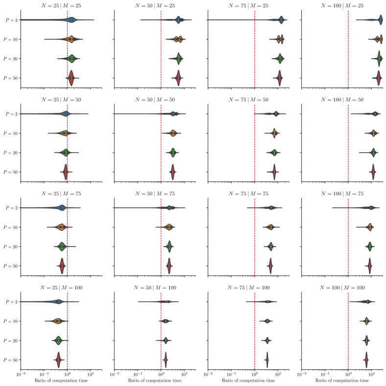
Figure 5: Ratio of computation time for Scenario 1 between the Gram matrix method and the covariance operator method. Each univariate component is defined on a one-dimensional domain. $N$ is the number of observations, $M$ is the number of sampling points per curve and $P$ is the number of features.

Figure 6 shows the kernel density estimates of the ratio of CT for each method across all sample sizes and number of sampling points. For Scenario 2, we found that the diagonalization of the Gram matrix has a shorter CT compared to the diagonalization of the covariance operator across all sample sizes and number of sampling points.

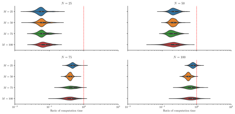
Figure 6: Ratio of computation time for Scenario 2 between the Gram matrix method and the covariance operator method. $N$ is the number of observations and $M\times M$ is the number of sampling points per images.

The shorter computational time of the diagonalization of the Gram matrix for Scenario 2 makes it a more efficient option for analyzing two and higher-dimensional functional datasets. It is however worth noting that the computational time can still vary depending on the specific implementation of each method, the computational resources available, and the complexity of the dataset (number of observations, number of sampling points, etc.).

Eigenvalues estimation. To compare the estimation of the eigenvalues between the diagonalization of the covariance operator and the diagonalization of the Gram matrix, we calculated the ratio of the $\log-\text{AE}$ (39) between the estimated eigenvalues and the true eigenvalues for each simulated dataset and for the first five eigenvalues. Figure 7 shows the boxplots of the $\log-\text{AE}$ for each method across all sample sizes, number of sampling points and number of features for Scenario 1. We found that the two methods behave similarly for all considered settings.

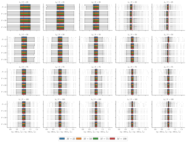
Figure 7: Ratio of $\log-$AE for Scenario 1 between the Gram matrix method and the covariance operator method. Each univariate component is defined on a one-dimensional domain. $N$ is the number of observations, $M$ is the number of sampling points per curve and $P$ is the number of features.

Figure 8 shows the boxplots of the $\log-\text{AE}$ for each method across all sample sizes and number of sampling points for Scenario 2. We found that the FCP-TPA gives slighty better estimation of the eigenvalues.

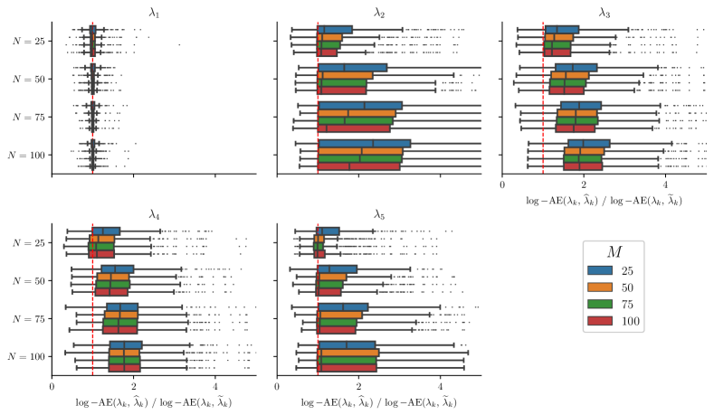
Figure 8: Ratio of $\log-$AE for Scenario 2 between the Gram matrix method and the covariance operator method. $N$ is the number of observations and $M\times M$ is the number of sampling points per images.

Eigenfunctions estimation. To compare the estimation of the eigenfunctions between the diagonalization of the covariance operator and the diagonalization of the Gram matrix, we calculated the ratio of the ISE (38) between the estimated eigenfunctions and the true eigenfunctions for each simulated dataset and for the first five eigenfunctions. Figure 9 shows the boxplots of the ISE for each method across all sample sizes, number of sampling points and number of features for Scenario 1. We found that the two methods behave similarly for all considered settings. For $P=10,20$ and $50$, the results are identical.

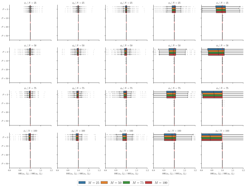
Figure 9: Ratio of ISE for Scenario 1 between the Gram matrix method and the covariance operator method. Each univariate component is defined on a one-dimensional domain. $N$ is the number of observations, $M$ is the number of sampling points per curve and $P$ is the number of features.

Figure 10 shows the boxplots of the ISE for each method across all sample sizes and number of sampling points for Scenario 2. We found that the decomposition of the Gram matrix gives better estimation of the eigenfunctions compared to the FCP-TPA, especially when the number of observations increases.

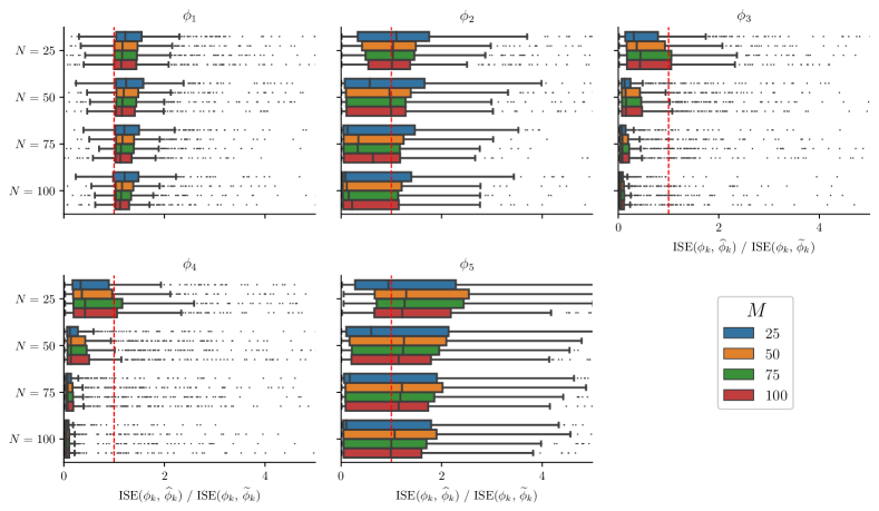
Figure 10: Ratio of ISE for Scenario 2 between the Gram matrix method and the covariance operator method. $N$ is the number of observations and $M\times M$ is the number of sampling points per images.

Curves reconstruction. To compare the quality of the reconstruction of the curves between the diagonalization of the covariance operator and the diagaonlisation of the Gram matrix, we calculated the ratio of the MISE (40) between the reconstruction of the curves and the true curves for each simulated dataset. Figure 11 shows the boxplots of the ISE for each method across all sample sizes, number of sampling points and number of features for Scenario 1. We found that the diagonalization of the Gram matrix gives slightly better results for all considered settings.

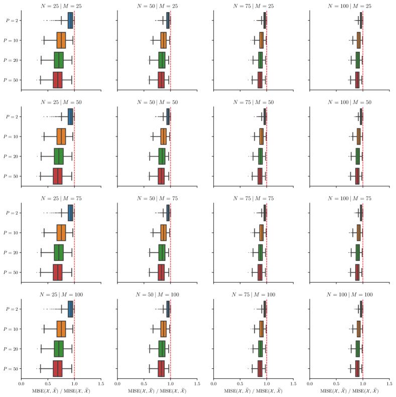
Figure 11: Ratio of MISE for Scenario 1 between the Gram matrix method and the covariance operator method. Each univariate component is defined on a one-dimensional domain. $N$ is the number of observations, $M$ is the number of sampling points per curve and $P$ is the number of features.

Figure 12 shows the boxplots of the ISE for each method across all sample sizes and number of sampling points for Scenario 2. Similarly to Scenario 1, we found that the decomposition of the Gram matrix gives better estimation of the true curves compared to the FCP-TPA, especially when the number of observations increases.

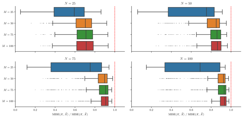
Figure 12: Ratio of MISE for Scenario 2 between the Gram matrix method and the covariance operator method. $N$ is the number of observations and $M\times M$ is the number of sampling points per images.

6 Discussion and conclusion

MFPCA is a fundamental statistical tool for the analysis of multivariate functional data, which enables us to capture the variability in observations defined by multiple curves. In this paper, we have described the duality between rows and columns of a data matrix within the context of multivariate functional data. We have proposed to use this duality to estimate the eigencomponents of the covariance operator in multivariate functional datasets. By comparing the results of the two methods, we provide the researcher with guidelines for determining the most appropriate method within a range of functional data frameworks. Overall, our simulations showed that the diagonalization of the covariance operator or of the Gram matrix gave similar results in terms of the estimation of the eigenvalues, the eigenfunctions and reconstruction of the curves for one-dimensional multivariate functional data, while the performance of the diagonalization of the Gram matrix outperformed the FCP-TPA for higher-dimensional functional datasets. Regarding the computation time, the use of the covariance operator is faster in most cases for multivariate functional data defined on unidimensional domains. The only situation where the use of the Gram matrix is quicker is when $M\gg N$. For data defined on higher-dimensional domains, diagonalization of the Gram matrix is faster. In conclusion, we recommend to use the covariance operator for multivariate functional data with all features defined on a one-dimensional domeins (curves) and for a number of observations larger or comparable to the number of sampling points regardless of the number of features. If the data are defined on multi-dimensional domains (images) or the number of sampling points is much higher than the number of observations, we advise using the Gram matrix.

Utilizing the Gram matrix enables the estimation of the number of components retained via the percentage of variance explained by the multivariate functional data, whereas the decomposition of the covariance operator necessitates the specification of the percentage of variance accounted for by each individual univariate feature. Specifying the percentage of variance explained for each feature does not guarantee that we recover the nominal percentage of variance explained for the multivariate data. Although we have not investigated the extent to which this might be important, the duality relation derived in this work provides a direct solution to the problem. Future work could investigate the settings in which univariate variance-explained cutoffs fail to retain the correct percentage of variance explained in multivariate functional data, and hence where the Gram matrix approach may be preferred.

In practice, observations of (multivariate) functional data are often subject to noise. As we recommend the use of the Gram matrix solely for densely sampled functional datasets, individual curve smoothing should suffice to approximate the Gram matrix in such cases. The estimation of the Gram matrix in the context of sparsely sampled functional data is however deemed irrelevant, given our findings that the utilization of the covariance operator for the estimation of the eigencomponents yields comparable results, while typically requiring less computational time.

The open-source implementation can be accessed at https://github.com/StevenGolovkine/FDApy, while scripts to reproduce the simulations are at https://github.com/FAST-ULxNUIG/geom_mfpca.

Appendix A Derivation of the equalities

Using the definition of adjoint operators, we must prove that

$$\left(L_{X}(f),u\right)_{\mathbf{M}}=\langle\!\langle f,L^{\star}_{X}(u)\rangle\!\rangle_{\Gamma},\quad\text{for all}\quad f\in\mathcal{H},\quad u\in\mathbb{R}^{N}.$$ (46)

For all $f\in\mathcal{H},u\in\mathbb{R}^{N}$, we have that

$$\left(L_{X}(f),u\right)_{\mathbf{M}} =L_{X}(f)^{\top}\mathbf{M}u$$

$$=\sum_{i=1}^{N}\sum_{j=1}^{N}\pi_{i}\sqrt{\pi_{j}}u_{j}\langle\!\langle X_{i}-\mu,X_{j}-\mu\rangle\!\rangle\langle\!\langle X_{i}-\mu,f\rangle\!\rangle,$$

$$\langle\!\langle f,L^{\star}_{X}(u)\rangle\!\rangle_{\Gamma} =\langle\!\langle\Gamma f,L^{\star}_{X}(u)\rangle\!\rangle$$

$$=\sum_{p=1}^{P}\int_{\mathcal{T}_{p}}(\Gamma f)^{(p)}(t_{p})\left\{\sum_{n=1}^{N}\sqrt{\pi_{n}}u_{n}\left(X_{n}^{(p)}(t_{p})-\mu^{(p)}(t_{p})\right)\right\}{\rm d}t_{p}$$

$$=\sum_{p=1}^{P}\int_{\mathcal{T}_{p}}\left\{\sum_{q=1}^{P}\int_{\mathcal{T}_{q}}C_{p,q}(t_{p},s_{q})f^{(q)}(s_{q}){\rm d}s_{q}\right\}\left\{\sum_{j=1}^{N}\sqrt{\pi_{j}}u_{j}\left(X_{j}^{(p)}(t_{p})-\mu^{(p)}(t_{p})\right)\right\}{\rm d}t_{p}$$

$$=\sum_{i=1}^{N}\sum_{j=1}^{N}\pi_{i}\sqrt{\pi_{j}}u_{j}\left\{\sum_{p=1}^{P}\int_{\mathcal{T}_{p}}\left(X_{i}^{(p)}(t_{p})-\mu^{(p)}(t_{p})\right)\left(X_{j}^{(p)}(t_{p})-\mu^{(p)}(t_{p})\right){\rm d}t_{p}\right\}\times$$

$$\qquad\qquad\left\{\sum_{q=1}^{P}\int_{\mathcal{T}_{q}}\left(X_{i}^{(q)}(s_{q})-\mu^{(q)}(s_{q})\right)f^{(q)}(s_{q}){\rm d}s_{q}\right\}$$

$$=\sum_{i=1}^{N}\sum_{j=1}^{N}\pi_{i}\sqrt{\pi_{j}}u_{j}\langle\!\langle X_{i}-\mu,X_{j}-\mu\rangle\!\rangle\langle\!\langle X_{i}-\mu,f\rangle\!\rangle.$$

So, the equality (46) is proved and we conclude that $L^{\star}_{X}$ is the adjoint operator of $L_{X}$.

Next, we derive the total inertia of the cloud $\mathcal{C}_{\!P}$ using the distance $d$. Recall that

$$\operatorname{Var}\{X^{(p)}(t_{p})\}=\sum_{n=1}^{N}\pi_{n}\{X_{n}^{(p)}(t_{p})\}^{2}-\{\mu^{(p)}(t_{p})\}^{2}\quad\text{where}\quad\mu^{(p)}(t_{p})=\sum_{n=1}^{N}\pi_{n}X_{n}^{(p)}(t_{p}),\quad t_{p}\in\mathcal{T}_{p}.$$ (47)

$$\sum_{n=1}^{N}\pi_{n}d^{2}(\mathrm{M}_{n},\mathrm{G}_{\!\mu}) =\sum_{n=1}^{N}\pi_{n}\sum_{p=1}^{P}\left|\!\left|X_{n}^{(p)}-\mu^{(p)}\right|\!\right|^{2}$$

$$=\sum_{p=1}^{P}\left(\sum_{n=1}^{N}\pi_{n}\left|\!\left|X_{n}^{(p)}\right|\!\right|^{2}-\left|\!\left|\mu^{(p)}\right|\!\right|^{2}\right)$$

$$=\sum_{p=1}^{P}\int_{\mathcal{T}_{p}}\operatorname{Var}{X^{(p)}(t_{p})}{\rm d}t_{p},$$

$$\sum_{i=1}^{N}\sum_{j=1}^{N}\pi_{i}\pi_{j}d^{2}(\mathrm{M}_{i},\mathrm{M}_{j}) =\sum_{i=1}^{N}\sum_{j=1}^{N}\pi_{i}\pi_{j}\sum_{p=1}^{P}\left|\!\left|X^{(p)}_{i}-X^{(p)}_{j}\right|\!\right|^{2}$$

$$=\sum_{p=1}^{P}\left(2\sum_{i=1}^{N}\pi_{i}\left|\!\left|X^{(p)}_{i}\right|\!\right|^{2}-2\sum_{i=1}^{N}\sum_{j=1}^{N}\pi_{i}\pi_{j}\left\langle X^{(p)}_{i},X^{(p)}_{j}\right\rangle\right)$$

$$=2\sum_{p=1}^{P}\int_{\mathcal{T}_{p}}\operatorname{Var}{X^{(p)}(t_{p})}{\rm d}t_{p}.$$

The equalities in Equation (21) are shown.

We now derive the total inertia of the cloud $\mathcal{C}_{\!P}$ using the distance $d_{\Gamma}$. We have that

$$\sum_{n=1}^{N}\pi_{n}d_{\Gamma}^{2}(\mathrm{M}_{n},\mathrm{G}_{\!\mu}) =\sum_{n=1}^{N}\pi_{n}\langle\!\langle X_{n}-\mu,X_{n}-\mu\rangle\!\rangle_{\Gamma}$$ (48)

$$=\sum_{n=1}^{N}\pi_{n}\left|\!\left|\!\left|X_{n}\right|\!\right|\!\right|_{\Gamma}^{2}-\left|\!\left|\!\left|\mu\right|\!\right|\!\right|_{\Gamma}^{2}$$ (49)

$$=\sum_{p=1}^{P}\left(\sum_{n=1}^{N}\pi_{n}\left|\!\left|X_{n}^{(p)}\right|\!\right|_{\Gamma}^{2}-\left|\!\left|\mu^{(p)}\right|\!\right|_{\Gamma}^{2}\right)$$ (50)

$$=\sum_{p=1}^{P}\sum_{q=1}^{P}\int_{\mathcal{T}_{p}}\int_{\mathcal{T}_{q}}C_{p,q}(t_{p},s_{q})C_{p,q}(t_{p},s_{q}){\rm d}s_{q}{\rm d}t_{p}$$ (51)

$$=\sum_{p=1}^{P}\int_{\mathcal{T}_{p}}\left|\!\left|\!\left|C_{p\cdot}(t_{p},\cdot)\right|\!\right|\!\right|^{2}{\rm d}t_{p},$$ (52)

$$\frac{1}{2}\sum_{i=1}^{N}\sum_{j=1}^{N}\pi_{i}\pi_{j}d_{\Gamma}^{2}(\mathrm{M}_{i},\mathrm{M}_{j}) =\sum_{i=1}^{N}\pi_{i}\left|\!\left|\!\left|X_{i}\right|\!\right|\!\right|_{\Gamma}^{2}-\sum_{i=1}^{N}\sum_{j=1}^{N}\pi_{i}\pi_{j}\langle\!\langle X_{i},X_{j}\rangle\!\rangle_{\Gamma}$$ (53)

$$=\sum_{i=1}^{N}\pi_{i}\left|\!\left|\!\left|X_{i}\right|\!\right|\!\right|_{\Gamma}^{2}-\left|\!\left|\!\left|\mu\right|\!\right|\!\right|_{\Gamma}^{2}$$ (54)

$$=\sum_{p=1}^{P}\int_{\mathcal{T}_{p}}\left|\!\left|\!\left|C_{p\cdot}(t_{p},\cdot)\right|\!\right|\!\right|^{2}{\rm d}t_{p}.$$ (55)

The equalities in Equation (23) are shown.

Finally, we derive the inertia of the cloud $\mathcal{C}_{\!N}$ using the distance $\mathsf{d}$. We have that

$$\sum_{n=1}^{N}\pi_{n}\mathsf{d}^{2}(\mathsf{M}_{n},\mathsf{G}_{\!\mu}) =\sum_{i=1}^{N}\sum_{j=1}^{N}\pi_{i}\pi_{j}\langle\!\langle X_{i}-\mu,X_{j}-\mu\rangle\!\rangle\langle\!\langle X_{i}-\mu,X_{j}-\mu\rangle\!\rangle$$ (56)

$$=\sum_{p=1}^{P}\sum_{q=1}^{P}\int_{\mathcal{T}_{p}}\int_{\mathcal{T}_{q}}C_{p,q}(t_{p},s_{q})C_{p,q}(t_{p},s_{q}){\rm d}s_{q}{\rm d}t_{p}$$ (57)

$$=\sum_{p=1}^{P}\int_{\mathcal{T}_{p}}\left|\!\left|\!\left|C_{p\cdot}(t_{p},\cdot)\right|\!\right|\!\right|^{2}{\rm d}t_{p},$$ (58)

$$\sum_{i=1}^{N}\sum_{j=1}^{N}\pi_{i}\pi_{j}\mathsf{d}^{2}(\mathsf{M}_{i},\mathsf{M}_{j}) =\sum_{i=1}^{N}\sum_{j=1}^{N}\sum_{n=1}^{N}\pi_{i}\pi_{j}\pi_{n}\langle\!\langle X_{n}-\mu,X_{i}-X_{j}\rangle\!\rangle\langle\!\langle X_{n}-\mu,X_{i}-X_{j}\rangle\!\rangle$$ (59)

$$=2\sum_{i=1}^{N}\sum_{j=1}^{N}\pi_{i}\pi_{j}\langle\!\langle X_{i}-\mu,X_{j}-\mu\rangle\!\rangle\langle\!\langle X_{i}-\mu,X_{j}-\mu\rangle\!\rangle$$ (60)

$$=2\sum_{p=1}^{P}\int_{\mathcal{T}_{p}}\left|\!\left|\!\left|C_{p\cdot}(t_{p},\cdot)\right|\!\right|\!\right|^{2}{\rm d}t_{p}.$$ (61)

The equalities in Equation (24) are shown.

Appendix B Derivation of the eigencomponents

Using the Hilbert-Schmidt theorem, there exists a complete orthonormal basis of eigenvectors $\{v_{k}\}_{1\leq k\leq N}$ of the inner-product matrix $\mathbf{M}$ such that

$$\mathbf{M}v_{k}=l_{k}v_{k}.$$ (62)

Let $X=\left(X_{1}-\mu,\dots,X_{N}-\mu\right)^{\top}$ and denote $\widetilde{X}=\text{diag}\{\sqrt{\pi_{1}},\dots,\sqrt{\pi_{N}}\}X$, the matrix of weighted observations. Recall that, in the case of $P$-dimensional process, the realisations of the process $X_{n},\leavevmode\nobreak\ n=1,\cdots,N$ and $\mu$ are vectors of functions of length $P$, and thus $X$ (and $\widetilde{X}$) is a matrix of functions of size $N\times P$. By left multiplying Equation (62) by $\widetilde{X}^{\top}$, we obtain

$$\widetilde{X}^{\top}\mathbf{M}v_{k}=l_{k}\widetilde{X}^{\top}v_{k}.$$ (63)

Expanding Equation (63), for each component $p=1,\dots,P$, we have,

$$\sum_{i=1}^{N}\sum_{j=1}^{N}\pi_{i}\sqrt{\pi_{j}}[v_{k}]_{j}\left\{X_{i}^{(p)}(\cdot)-\mu^{(p)}(\cdot)\right\}\langle\!\langle X_{i}-\mu,X_{j}-\mu\rangle\!\rangle=l_{k}\mkern-5.0mu\sum_{n=1}^{N}\mkern-4.0mu\sqrt{\pi_{n}}[v_{k}]_{n}\left\{X_{n}^{(p)}(\cdot)-\mu^{(p)}(\cdot)\right\}.$$ (64)

Here and in the following, we note $[a]_{p}$ the $p$th entry of the vector $a$. Starting from the left side of Equation (64), we get

$$[\widetilde{X}^{\top}\mathbf{M}v_{k}]_{p} =\sum_{i=1}^{N}\sum_{j=1}^{N}\pi_{i}\sqrt{\pi_{j}}[v_{k}]_{j}\left\{X_{i}^{(p)}(\cdot)-\mu^{(p)}(\cdot)\right\}\langle\!\langle X_{i}-\mu,X_{j}-\mu\rangle\!\rangle$$ (65)

$$=\sum_{q=1}^{P}\int_{\mathcal{T}_{q}}\sum_{i=1}^{N}\pi_{i}\left\{X_{i}^{(p)}(\cdot)-\mu^{(p)}(\cdot)\right\}\left\{X_{i}^{(q)}(s_{q})-\mu^{(q)}(s_{q})\right\}$$ (66)

$$\qquad\qquad\sum_{j=1}^{N}\sqrt{\pi_{j}}[v_{k}]_{j}\left\{X_{j}^{(q)}(s_{q})-\mu^{(q)}(s_{q})\right\}{\rm d}s_{q}$$ (67)

$$=\sum_{q=1}^{P}\int_{\mathcal{T}_{q}}C_{p,q}(\cdot,s_{q})\sum_{j=1}^{N}\sqrt{\pi_{j}}[v_{k}]_{j}\left\{X_{j}^{(q)}(s_{q})-\mu^{(q)}(s_{q})\right\}{\rm d}s_{q}$$ (68)

$$=\sum_{j=1}^{N}\langle\!\langle C_{p\cdot}(\cdot,\cdot),\sqrt{\pi_{j}}[v_{k}]_{j}\left\{X_{j}-\mu\right\}\rangle\!\rangle$$ (69)

$$=\Gamma\left(\sum_{j=1}^{N}\sqrt{\pi_{j}}[v_{k}]_{j}\left\{X_{j}-\mu\right\}\right)^{\mkern-9.0mu(p)}\mkern-18.0mu(\cdot),$$ (70)

and, starting from the right side of Equation (64),

$$[l_{k}\widetilde{X}^{\top}v_{k}]_{p}=l_{k}\sum_{n=1}^{N}\sqrt{\pi_{n}}[v_{k}]_{n}\left\{X_{n}^{(p)}(\cdot)-\mu^{(p)}(\cdot)\right\}.$$ (71)

From Equation (65) and Equation (71), we obtain

$$\Gamma\left(\sum_{j=1}^{N}\sqrt{\pi_{j}}[v_{k}]_{j}\left\{X_{j}-\mu\right\}\right)^{\mkern-9.0mu(p)}\mkern-18.0mu(\cdot)=l_{k}\sum_{n=1}^{N}\sqrt{\pi_{n}}[v_{k}]_{n}\left\{X_{n}^{(p)}(\cdot)-\mu^{(p)}(\cdot)\right\},\quad\text{for all}\leavevmode\nobreak\ p=1,\dots,P.$$ (72)

By identification in Equation (29), we find that, for each components $p$,

$$\lambda_{k}=l_{k}\quad\text{and}\quad\phi_{k}^{(p)}(\cdot)=\sum_{n=1}^{N}\sqrt{\pi_{n}}[v_{k}]_{n}\left\{X_{n}^{(p)}(\cdot)-\mu^{(p)}(\cdot)\right\},\quad k\geq 1.$$ (73)

For $k\geq 1$, the norm of the eigenfunction is computed as the following:

$$\left|\!\left|\!\left|\phi_{k}\right|\!\right|\!\right|^{2} =\sum_{i=1}^{N}\sum_{j=1}^{N}\sqrt{\pi_{i}\pi_{j}}[v_{k}]_{i}[v_{k}]_{j}\langle\!\langle X_{i}-\mu,X_{j}-\mu\rangle\!\rangle=\sum_{i=1}^{N}[v_{k}]_{i}\sum_{j=1}^{N}\mathbf{M}_{ij}[v_{k}]_{j}$$

$$=\sum_{i=1}^{N}[v_{k}]_{i}l_{k}[v_{k}]_{i}=l_{k}\left|\!\left|v_{k}\right|\!\right|^{2}=l_{k}.$$

Therefore, in order to have an orthonormal basis of eigenfunctions, we normalise the eigenfunctions $\phi_{k}$ from Equation (73) by $1/\sqrt{l_{k}}$. Concerning the estimation of the scores, for $n=1,\dots,N$, for $k\geq 1$, we have

$$\mathfrak{c}_{nk} =\langle\!\langle X_{n}-\mu,\phi_{k}\rangle\!\rangle=\frac{1}{\sqrt{l_{k}}}\sum_{j=1}^{N}\sqrt{\pi_{j}}[v_{k}]_{j}\langle\!\langle X_{n}-\mu,X_{j}-\mu\rangle\!\rangle$$ (74)

$$=\frac{1}{\sqrt{l_{k}\pi_{n}}}\sum_{j=1}^{N}[v_{k}]_{j}\mathbf{M}_{nj}=\sqrt{\frac{l_{k}}{\pi_{n}}}[v_{k}]_{n}.$$ (75)

Concerning the expansion of the data into the basis of function $\Psi$, we write

$$\mathbf{M}=\left(\text{diag}\{\sqrt{\pi_{1}},\dots,\sqrt{\pi_{N}}\}\left(\mathrm{I}_{\!N}-\mathbf{1}_{\!N}\Pi^{\top}\right)\mathbf{C}W^{1/2}\right)\left(\text{diag}\{\sqrt{\pi_{1}},\dots,\sqrt{\pi_{N}}\}\left(\mathrm{I}_{\!N}-\mathbf{1}_{\!N}\Pi^{\top}\right)\mathbf{C}W^{1/2}\right)^{\top}.$$ (77)

We note

$$\mathbf{A}=\text{diag}\{\sqrt{\pi_{1}},\dots,\sqrt{\pi_{N}}\}\left(\mathrm{I}_{\!N}-\mathbf{1}_{\!N}\Pi^{\top}\right)\mathbf{C}W^{1/2},$$ (78)

such that $\mathbf{M}=\mathbf{A}\mathbf{A}^{\top}$. We also assume that $\phi_{1},\phi_{2},\dots$ the eigenfunctions of the covariance operator $\Gamma$ have a decomposition into the basis $\Psi$

$$\phi_{k}(\cdot)=\begin{pmatrix}\phi_{k}^{(1)}(\cdot)\\ \vdots\\ \phi_{k}^{(P)}(\cdot)\end{pmatrix}=\begin{pmatrix}\psi^{(1)\top}(\cdot)b_{1k}\\ \vdots\\ \psi^{(P)\top}(\cdot)b_{Pk}\end{pmatrix},\quad\text{where}\quad b_{pk}=\left(b_{pk1},\dots,b_{pkK_{p}}\right)^{\top}.$$ (79)

We have, for $p=1,\dots,P$,

$$\left(\Gamma\phi_{k}\right)^{(p)}(\cdot) =\sum_{q=1}^{P}\int_{\mathcal{T}_{q}}C_{p,q}(\cdot,s_{q})\phi_{k}^{(q)}(s_{q}){\rm d}s_{q}$$

$$=\sum_{q=1}^{P}\int_{\mathcal{T}_{q}}\Psi(\cdot)^{(p)\top}\mathbf{C}^{(p)\top}\left(\text{diag}\{\pi_{1},\dots,\pi_{N}\}-\Pi\Pi^{\top}\right)\mathbf{C}^{(q)}\Psi^{(q)}(s_{q})\Psi^{(q)}(s_{q})^{\top}b_{qk}{\rm d}s_{q}$$

$$=\Psi(\cdot)^{(p)\top}\mathbf{C}^{(p)\top}\left(\text{diag}\{\pi_{1},\dots,\pi_{N}\}-\Pi\Pi^{\top}\right)\sum_{q=1}^{P}\mathbf{C}^{(q)}\int_{\mathcal{T}_{q}}\Psi^{(q)}(s_{q})\Psi(s_{q})^{(q)\top}{\rm d}s_{q}b_{qk}$$

$$=\Psi(\cdot)^{(p)\top}\mathbf{C}^{(p)\top}\left(\text{diag}\{\pi_{1},\dots,\pi_{N}\}-\Pi\Pi^{\top}\right)\sum_{q=1}^{P}\mathbf{C}^{(q)}\mathbf{W}^{(q)}b_{qk}.$$

This equation is true for all $p=1,\cdots,P$, this can be rewritten with matrices as

$$\Gamma\phi_{k}(\cdot)=\Psi(\cdot)^{\top}\mathbf{C}^{\top}\left(\text{diag}\{\pi_{1},\dots,\pi_{N}\}-\Pi\Pi^{\top}\right)\mathbf{C}\mathbf{W}b_{k}.$$ (80)

From the eigenequation, we have that

$$\Gamma\phi_{k}(\cdot)=\lambda_{k}\phi_{k}(\cdot)\Longleftrightarrow\Psi(\cdot)^{\top}\mathbf{C}^{\top}\left(\text{diag}\{\pi_{1},\dots,\pi_{N}\}-\Pi\Pi^{\top}\right)\mathbf{C}\mathbf{W}b_{k}=\lambda_{k}\Psi(\cdot)^{\top}b_{k}.$$ (81)

Since this equation must be true for all $t_{p}\in\mathcal{T}_{p}$, this imply the equation

$$\mathbf{C}^{\top}\left(\text{diag}\{\pi_{1},\dots,\pi_{N}\}-\Pi\Pi^{\top}\right)\mathbf{C}\mathbf{W}b_{k}=\lambda_{k}b_{k}.$$ (82)

As the eigenfunctions are assumed to be normalized, $\left|\!\left|\!\left|\phi_{k}\right|\!\right|\!\right|^{2}=1$. And so, $b_{k}^{\top}Wb_{k}=1$. Let $u_{k}=W^{1/2}b_{k}$. Then, from Equation (82), we obtain

$$\mathbf{W}^{1/2}\mathbf{C}^{\top}\left(\text{diag}\{\pi_{1},\dots,\pi_{N}\}-\Pi\Pi^{\top}\right)\mathbf{C}\mathbf{W}^{1/2}u_{k}=\lambda_{k}u_{k}\Longleftrightarrow\mathbf{A}^{\top}\mathbf{A}u_{k}=N\lambda_{k}u_{k}.$$ (83)

From the eigendecomposition of the matrix $M$, we get

$$\mathbf{M}v_{k}=l_{k}v_{k}\Longleftrightarrow\mathbf{A}\mathbf{A}^{\top}v_{k}=l_{k}v_{k}.$$ (84)

The equations (83) and (84) are eigenequations in the classical PCA case, with the duality $X^{\top}X$ and $XX^{\top}$. Following Pagès, (2014); Härdle and Simar, (2019), we find that, for $1\leq k\leq K$,

$$\lambda_{k}=l_{k},\quad v_{k}=\frac{1}{\sqrt{l_{k}}}\mathbf{A}u_{k}\quad\text{and}\quad u_{k}=\frac{1}{\sqrt{l_{k}}}\mathbf{A}^{\top}v_{k}.$$ (85)

And finally, to get the coefficient of the eigenfunctions, for $1\leq k\leq K$,

$$b_{k}=\mathbf{W}^{-1/2}u_{k}=\frac{1}{\sqrt{l_{k}}}\mathbf{C}^{\top}\left(\mathrm{I}_{\!N}-\Pi\mathbf{1}_{\!N}^{\top}\right)\text{diag}\{\sqrt{\pi_{1}},\dots,\sqrt{\pi_{N}}\}v_{k}.$$ (86)

References

- Allen, (2013) Allen, G. I. (2013). Multi-way functional principal components analysis. In 2013 5th IEEE International Workshop on Computational Advances in Multi-Sensor Adaptive Processing (CAMSAP), pages 220–223.
- Benko et al., (2009) Benko, M., Härdle, W., and Kneip, A. (2009). Common functional principal components. The Annals of Statistics, 37(1):1–34.
- Berrendero et al., (2011) Berrendero, J., Justel, A., and Svarc, M. (2011). Principal components for multivariate functional data. Computational Statistics & Data Analysis, 55:2619–2634.
- Berrendero et al., (2020) Berrendero, J. R., Bueno-Larraz, B., and Cuevas, A. (2020). On Mahalanobis Distance in Functional Settings. Journal of Machine Learning Research, 21(9):1–33.
- Chen et al., (2017) Chen, K., Zhang, X., Petersen, A., and Müller, H.-G. (2017). Quantifying Infinite-Dimensional Data: Functional Data Analysis in Action. Statistics in Biosciences, 9(2):582–604.
- Chiou et al., (2014) Chiou, J.-M., Chen, Y.-T., and Yang, Y.-F. (2014). Multivariate Functional Principal Component Analysis: A Normalization Approach. Statistica Sinica, 24(4):1571–1596.
- Dauxois et al., (1982) Dauxois, J., Pousse, A., and Romain, Y. (1982). Asymptotic theory for the principal component analysis of a vector random function: Some applications to statistical inference. Journal of Multivariate Analysis, 12(1):136–154.
- De la Cruz and Holmes, (2011) De la Cruz, O. and Holmes, S. (2011). The Duality Diagram in Data Analysis: Examples of Modern Applications. The annals of applied statistics, 5(4):2266–2277.
- Escofier, (1979) Escofier, B. (1979). Traitement simultané de variables qualitatives et quantitatives en analyse factorielle. Cahiers de l’analyse des données, 4(2):137–146.
- González and Muñoz, (2010) González, J. and Muñoz, A. (2010). Representing functional data in reproducing Kernel Hilbert Spaces with applications to clustering and classification. DES - Working Papers. Statistics and Econometrics. WS, (ws102713).
- Happ and Greven, (2018) Happ, C. and Greven, S. (2018). Multivariate Functional Principal Component Analysis for Data Observed on Different (Dimensional) Domains. Journal of the American Statistical Association, 113(522):649–659.
- Happ-Kurz, (2020) Happ-Kurz, C. (2020). Object-Oriented Software for Functional Data. Journal of Statistical Software, 93(1):1–38.
- Härdle and Simar, (2019) Härdle, W. K. and Simar, L. (2019). Applied Multivariate Statistical Analysis. Springer Nature.
- Holmes, (2008) Holmes, S. (2008). Multivariate data analysis: The French way. Probability and Statistics: Essays in Honor of David A. Freedman, 2:219–234.
- Horvàth and Kokoszka, (2012) Horvàth, L. and Kokoszka, P. (2012). Inference for Functional Data with Applications. Springer Series in Statistics.
- Jacques and Preda, (2014) Jacques, J. and Preda, C. (2014). Model-based clustering for multivariate functional data. Computational Statistics & Data Analysis, 71:92–106.
- Karhunen, (1947) Karhunen, K. (1947). Über lineare Methoden in der Wahrscheinlichkeitsrechnung. PhD thesis, (Sana), Helsinki.
- Kneip and Utikal, (2001) Kneip, A. and Utikal, K. J. (2001). Inference for Density Families Using Functional Principal Component Analysis. Journal of the American Statistical Association, 96(454):519–532.
- Kokoszka et al., (2017) Kokoszka, P., Oja, H., Park, B., and Sangalli, L. (2017). Special issue on functional data analysis. Econometrics and Statistics, 1:99–100.
- Krzyśko et al., (2022) Krzyśko, M., Nijkamp, P., Ratajczak, W., and Wołyński, W. (2022). Multidimensional economic indicators and multivariate functional principal component analysis (MFPCA) in a comparative study of countries’ competitiveness. Journal of Geographical Systems, 24(1):49–65.
- Loève, (1945) Loève, M. (1945). Sur les fonctions aléatoires stationnaires de second ordre. La Revue Scientifique, 5. Série, 83:297–303.
- Martino et al., (2019) Martino, A., Ghiglietti, A., Ieva, F., and Paganoni, A. M. (2019). A k-means procedure based on a Mahalanobis type distance for clustering multivariate functional data. Statistical Methods & Applications, 28(2):301–322.
- Pagès, (2014) Pagès, J. (2014). Multiple Factor Analysis by Example Using R. CRC Press.
- Prothero et al., (2023) Prothero, J., Hannig, J., and Marron, J. S. (2023). New Perspectives on Centering. The New England Journal of Statistics in Data Science, pages 1–21.
- Ramsay and Silverman, (2005) Ramsay, J. and Silverman, B. W. (2005). Functional Data Analysis. Springer Science & Business Media.
- Ramsay, (1982) Ramsay, J. O. (1982). When the data are functions. Psychometrika, 47(4):379–396.
- Reed and Simon, (1980) Reed, M. and Simon, B. (1980). Methods of Modern Mathematical Physics: Functional Analysis. Academic Press.
- Saporta, (1990) Saporta, G. (1990). Simultaneous Analysis of Qualitative and Quantitative Data. Atti 35° Riunione Scientifica della Societa Italiana di Statistica, pages pp. 63–72.
- Song and Kim, (2022) Song, J. and Kim, K. (2022). Sparse multivariate functional principal component analysis. Stat, 11(1):e435.
- Wang et al., (2016) Wang, J.-L., Chiou, J.-M., and Müller, H.-G. (2016). Functional Data Analysis. Annual Review of Statistics and Its Application, 3(1):257–295.
- Warmenhoven et al., (2019) Warmenhoven, J., Cobley, S., Draper, C., Harrison, A., Bargary, N., and Smith, R. (2019). Bivariate functional principal components analysis: Considerations for use with multivariate movement signatures in sports biomechanics. Sports Biomechanics, 18(1):10–27.
- Wong and Zhang, (2019) Wong, R. K. W. and Zhang, X. (2019). Nonparametric operator-regularized covariance function estimation for functional data. Computational Statistics & Data Analysis, 131:131–144.