Logarithmic or algebraic: roughening of an active Kardar-Parisi-Zhang surface

Abstract

The Kardar-Parisi-Zhang (KPZ) equation sets the universality class for growing and roughening of nonequilibrium surfaces without any conservation law and nonlocal effects. We argue here that the KPZ equation can be generalised by including a symmetry-permitted nonlocal nonlinear term of active origin that is of the same order as the one included in the KPZ equation. Including this term, the 2D active KPZ equation is stable in some parameter regimes, in which the interface conformation fluctuations exhibit sub-logarithmic or super-logarithmic roughness, with nonuniversal exponents, giving positional generalised quasi-long-ranged order. For other parameter choices, the model is unstable, suggesting a perturbatively inaccessible algebraically rough interface or positional short-ranged order. Our model should serve as a paradigmatic nonlocal growth equation.

The Kardar-Parisi-Zhang (KPZ) equation Kardar et al. (1986); Krug (1997); Barabási and Stanley (1995) for growing nonequilibrium surfaces displays a nonequilibrium roughening transition between a smooth phase, whose long wavelength scaling properties are identical to an Edward-Wilkinson (EW) surface Edwards and Wilkinson (1982) at the same dimension $d$, to a perturbatively inaccessible rough surface Barabási and Stanley (1995); Tang et al. (1990) when $d>d_{c}=2$, its lower critical dimension. Importantly, its local surface growth velocity that depends locally on surface fluctuations, and hence cannot describe nonequilibrium surface dynamics with nonlocal interactions.

Theoretical studies on nonlocal interactions has a longstanding history in equilibrium systems Fisher et al. (1972); Frey and Schwabl (1994); Bayong et al. (1999); Aronovitz and Lubensky (1988); Banerjee et al. (2019a, b). Examples of their prominent nonequilibrium counterparts include interface dynamics involving nonlocal interactions, e.g., flame front propagation, thin film growth Pelcé et al. (2004). Monte-Carlo simulation studies on a solid-on-solid model with nonlocal effects Ketterl and Hagston (1999) reveal how the shading phenomena in surface growth is described by nonlocal effects. Furthermore, kinetic roughening in the presence of nonlocal interactions Mukherji and Bhattacharjee (1997) display generic non-KPZ scaling behaviour. Nonlocal effects are often important in biological growth processes; see, e.g., Ref. Santalla and Ferreira (2018) for a recent study. Furthermore in many applications, the growth is controlled by fast nonlocal transport, not included in the KPZ equation. Prominent examples include diffusion-controlled nonlocal transport Aharonov and Rothman (1996), dissolution or precipitation processes Lichtner et al. (1996), gas-solid reactions Doǧu (1981), and a variety of reaction engineering processes Delmono and Froment (1999). Yet another potentially relevant example is diffusion-limited erosion, that displays nonlocal stabilisation of surfaces Krug and Meakin (1991); see also Ref. Nicoli et al. (2009). Nonlocal effects may be vital even in geological contexts, e.g., earth surface roughness R. Schumer (2017). Inspired by these past studies, we explore the generic consequences of competition between local contributions and those that depend on the global surface profile, i.e., nonlocal contributions to the local surface velocity, by constructing a purpose-built conceptual model.

In this Letter, we set up and study a generalisation of the KPZ equation, where the surface velocity depends, in contrast to the KPZ equation, nonlocally on the surface fluctuations. We do this by adding a symmetry-permitted nonlocal nonlinear gradient term that is of the same order as the usual KPZ nonlinear term. This allows us to study competition between local and nonlocal nonlinear effects. To generalise the scope of our study, we also include chiral contributions, which is ubiquitous in soft matter and biologically inspired systems; see, e.g., Refs. Martin et al. (2021); Lalitha et al. (2001). The resulting equation in 2D, named active-KPZ or a-KPZ equation is

$$\frac{\partial h}{\partial t}= \nu\nabla^{2}h+\frac{\lambda}{2}(\bm{\nabla}h)^{2}+\lambda_{1}Q_{ij}({\bf r})(\nabla_{i}h\nabla_{j}h)$$ (1)

$$+\lambda_{2}Q_{ij}({\bf r})e_{jm}(\nabla_{i}h\nabla_{m}h)+\eta,$$

a nonlocal generalisation to the usual KPZ equation that is distinct from the one considered in Ref. Mukherji and Bhattacharjee (1997). Here, the tensor $e_{jm}$ is the 2D totally antisymmetric matrix. Further, $Q_{ij}({\bf r})$ is the longitudinal projection operator that in the Fourier space is $Q_{ij}({\bf k})=k_{i}k_{j}/k^{2}$, where ${\bf k}$ is a Fourier wavevector, and is nonlocal. Physically $\lambda_{1}Q_{ij}({\bf r})(\nabla_{i}h\nabla_{j}h)+\lambda_{2}Q_{ij}({\bf r})e_{jm}(\nabla_{i}h\nabla_{m}h)$ is the contribution to the surface velocity normal to the base plane $v_{p}=\partial h/\partial t$ that is nonlocal in height fluctuations ${\bm{\nabla}}h$. Noise $\eta$ is a zero-mean, Gaussian-distributed white noise with a variance $\langle\eta({\bf x},t)\eta(0,0)\rangle=2D\delta^{d}({\bf x})\delta(t)$. We extract the scaling of the stable phases, which exists for a range of the model parameters. In particular, we show that the variance $\Delta\equiv\langle h({\bf x},t)^{2}\rangle\sim[\ln(L/a)]^{\mu}$ for a surface of lateral size $L$, where $\mu<(>)1$ for sub-(super-)logarithmic roughness and $a$ is a microscopic cutoff. This defines positional generalised quasi-long-ranged order (QLRO), generalising the well-known QLRO of EW surfaces Barabási and Stanley (1995), in which $\Delta\sim\ln(L/a)$, i.e., $\mu=1$. Further, the time-scale of relaxation $\tau(L)\sim L^{2}\,(\ln\,L)^{-\kappa},\,\kappa>0$, i.e., logarithmically superdiffusive. Both $\mu$ and $\kappa$ are non-universal: They vary continuously with $\lambda_{1}/\lambda,\,\lambda_{2}/\lambda$.

The form of Eq. (15) can be obtained by first considering the mapping from the KPZ equation to the Burgers equation Forster et al. (1977) in terms of the “Burgers velocity ${\bf v}={\bm{\nabla}}h$”. Now generalise the Burgers equation nonlinearity $\lambda{\bm{\nabla}}v^{2}$ to $\lambda_{1}\nabla_{j}(v_{i}v_{j})+\lambda_{2}e_{jm}\nabla_{j}(v_{i}v_{m})$, and then writing them in terms of $h$ produces the $\lambda_{1}$- and $\lambda_{2}$-terms in (15); see Supplemental Material (SM).

The $\lambda_{1}$- and $\lambda_{2}$-terms in (15) can be motivated by considering a nearly flat nonequilibrium surface described by a single valued height field $h({\bf x},t)$ in Monge gauge  Chaikin and Lubensky (2000); Nelson et al. (1989), with an active conserved density $\rho({\bf x},t)$ living on it. Its hydrodynamic equation, retaining only the lowest order in nonlinearities and spatial gradients, reads

$$\frac{\partial h}{\partial t}=\nu\nabla^{2}h+\frac{\lambda}{2}({\bm{\nabla}}h)^{2}+v(\rho)+\eta,$$ (2)

where $v(\rho)$ is a local density-dependent velocity of the membrane; $v(\rho)=v_{0}+g_{1}\rho$ to the leading order in $\rho$; $g_{1}$ is a coupling constant of either sign. Further, density $\rho$ follows $\partial_{t}\rho=-{\bm{\nabla}}\cdot{\bf J}$, where $\bf J$ is the current. The specific form of the particle dynamics decides the structure of $\bf J$. We choose ${J_{i}}=-\overline{D}{\nabla_{i}}\rho+{\nabla_{j}}\sigma_{ij}$, where $\sigma_{ij}\equiv\alpha\nabla_{i}h\nabla_{j}h+\beta e_{jm}\nabla_{i}h\nabla_{m}h$ is reminiscent of “active stresses” found in active matter theories Marchetti et al. (2013), the $\beta$-term is a chiral contribution. The quadratic dependence of $\bf J$ on ${\bm{\nabla}}h$ implies the active particles (i) respond, unsurprisingly, to the height fluctuations, but not the absolute height, and (ii) ignoring gravity, the particles do not distinguish valleys from the hills (although the surface itself breaks the inversion symmetry). Here, $\overline{D}>0$ is a diffusivity. We focus on the quasi-static limit of infinitely fast dynamics of $\rho$, such that $\partial\rho/\partial t\approx 0$, giving $\overline{D}\nabla^{2}\rho=\alpha\nabla_{i}\nabla_{j}(\nabla_{i}h\nabla_{j}h)+\beta e_{jm}\nabla_{i}\nabla_{j}(\nabla_{i}h\nabla_{m}h)$ neglecting any noise in the $\rho$-dynamics. Now use this to eliminate $\rho$ in (2) to get (15), after absorbing a factor of $\overline{D}$. (We have implicitly assumed $\alpha,\beta$ to scale with $\overline{D}$, and ignored any advective-type nonlinearity originating from projecting the particle dynamics on the plane of the membrane in the large $\overline{D}$-limit.) All of $\lambda,\lambda_{1},\lambda_{2}$ can be individually positive and negative. The chiral term is 2D specific; the other two nonlinear terms with coefficients $\lambda$ and $\lambda_{1}$ can exist in any dimension $d$. Thus the $\lambda_{1}$- and $\lambda_{2}$-terms in (15) are physical, although our active species origin need not be the only possible source of these two terms. See Ref. Rasshofer et al. (2022) for a similar mechanism to generate an effective nonlocal dynamics in the noisy Fisher-Kolmogorov equation FISHER (1937); Kolmogorov et al. (1937) for population dynamics coupled with a fast chemical signal. Further Eq. (15) can be realised microscopically by considering an “active” 2D single-step model for a 2D KPZ surface with point particles living on it. The dynamical update rules of the modified single-step model now depend on the local excess or deficit population of the active particles, instead of being constants as they are in standard single-step models Meakin et al. (1986); Plischke et al. (1987); Liu and Plischke (1988); Kondev et al. (2000); Naserabadi et al. (2017). The particle hopping rates to the nearest neighbour sites in turn depends not only on the number inhomogeneities, but also on the height fluctuations (but without distinguishing local valleys from hills). Monte-Carlo simulations of this model, focusing on the limiting case of fast dynamics by the number fluctuations, should bring out the physics described in this Letter. The limit of fast particle dynamics can be implemented by considering time-scale separations in the rates of particle position updates and surface conformation updates.

At one dimension, the $\lambda_{2}$-term vanishes, and the $\lambda_{1}$-term becomes indistinguishable from the $\lambda$-term. The transformation $x_{i}^{\prime}=x_{i}-(\lambda+2\lambda_{1})c_{i}t-\lambda_{2}e_{ij}c_{j}t$ and $t^{\prime}=t$, together with the height function $h$ transforming as $h^{\prime}({\bf x}^{\prime},t^{\prime})=h({\bf x},t)+\textbf{c}\cdot\textbf{x}$ leaves Eq. (15) invariant; see SM. This generalises invariance of the usual KPZ equation under a pseudo-Galilean transformation Barabási and Stanley (1995).

Similar to the KPZ equation, dimensional analysis via scaling ${\bf r}\rightarrow b{\bf r},\,t\rightarrow b^{z}t,\,h\rightarrow b^{\chi}h$, where $z$ and $\chi$ are the dynamic and roughness exponents, all of $\lambda,\lambda_{1},\lambda_{2}$ scale similarly, and $d=2$ is the critical dimension of Eq. (15); see SM. Whether it is the upper or lower critical dimension requires further analysis that follows below.

We first determine if Eq. (15) has a stable nonequilibrium steady state (NESS), and second, if so, the scaling properties in those NESS. We use renormalisation group (RG) framework, well-suited to systematically handle the diverging corrections encountered in naïve perturbation theories. The dynamic RG method for our model closely resembles that for the KPZ equation Kardar et al. (1986); Barabási and Stanley (1995); Täuber (2014).

We perform the Wilson momentum shell dynamic RG procedure at the one-loop order Barabási and Stanley (1995); Täuber (2014); Forster et al. (1977); see SM for the one-loop Feynman diagrams. There are no one-loop corrections to $\lambda,\lambda_{1},\lambda_{2}$. However, there are diverging one-loop corrections to $\nu$ and $D$. Dimensional analysis allows us to identify an effective dimensionless coupling constant $g$ and two dimensionless ratios $\gamma_{1},\,\gamma_{2}$ defined as $g\equiv\frac{\lambda^{2}D}{\nu^{3}}\frac{1}{2\pi},\,\gamma_{1}\equiv\frac{\lambda_{1}}{\lambda},\,\gamma_{2}\equiv\frac{\lambda_{2}}{\lambda}$. By following the standard steps of RG, we obtain the RG recursion relations for $D,\,\nu$ at the one-loop order (here $l$ is the “RG time”; $\exp(l)$ is a length-scale):

$$\frac{dD}{dl}=D\Bigr{[}z-d-2\chi+g{\cal B}(\gamma_{1},\gamma_{2})\Bigr{]},$$ (3)

$$\frac{d\nu}{dl}=\nu\Bigr{[}z-2+g{\cal C}(\gamma_{1},\gamma_{2})\Bigr{]},$$ (4)

with $\gamma_{1},\,\gamma_{2}$ being marginal at the one-loop order, stemming from the nonrenormalisation of $\lambda,\lambda_{1},\lambda_{2}$ at that order. Equations (3)-(4) are invariant under the inversion of $\lambda_{2}$, i.e., interchange of left handed coordinate system with a right handed one.Here, ${\cal B}[\gamma_{1},\gamma_{2}]=\frac{3}{8}\gamma_{1}^{2}+\frac{1}{2}\gamma_{1}+\frac{1}{8}\gamma_{2}^{2}+\frac{1}{4},\,{\cal C}[\gamma_{1},\gamma_{2}]=\frac{1}{2}\gamma_{1}^{2}+\frac{5}{8}\gamma_{1}+\frac{1}{8}\gamma_{2}^{2}$; ${\cal B}>0$. Flow equations (3)-(4) yield the flow equation for $g$:

$$\frac{dg}{dl}=-g^{2}{\cal A}[\gamma_{1},\gamma_{2}],$$ (5)

where ${\cal A}[\gamma_{1},\gamma_{2}]=\frac{9}{8}\gamma_{1}^{2}+\frac{11}{8}\gamma_{1}+\frac{1}{4}\gamma_{2}^{2}-\frac{1}{4}$.

We first focus on the achiral case, i.e., $\gamma_{2}=0$. An RG flow diagram in the $g-\gamma_{1}$ plane is shown in Fig. 1(a). The condition ${\cal\tilde{A}}(\gamma_{1})\equiv{\cal A}(\gamma_{1},\gamma_{2}=0)=0$ defines two solid (black) lines $\gamma_{1}=\gamma_{+},\,\gamma_{-}$ parallel to the $g$-axis in the $g-\gamma_{1}$ plane, where $\gamma_{+}=0.161,\gamma_{-}=-1.383$, such that for $\gamma_{+}>\gamma_{1}>\gamma_{-}$ (gray region), the RG flow lines flow away parallel to the $g$-axis towards infinity, indicating a perturbatively inaccessible, presumably rough, phase with short-ranged positional order. In this unstable region $g(l)$ diverges as $l\rightarrow 1/[|{\cal\tilde{A}}(\gamma_{1})|]$, reminiscent of the 2D KPZ equation Barabási and Stanley (1995), presumably corresponding to algebraically rough phase Basu and Frey (2004); Gomes-Filho et al. (2021). Outside this region, where ${\cal\tilde{A}}(\gamma_{1})>0$, the flow lines flow towards $g=0$ parallel to the $g$-axis, implying stability, with $g(l)\approx 1/[l{\cal\tilde{A}}(\gamma_{1})]$ vanishes slowly in the long wavelength limit $l\rightarrow\infty$. Although $g^{*}=0$ is the only fixed point (FP) in the stable region, the vanishing of $g(l)$ is so slow, being proportional to $1/l$, the parameters $D$ and $\nu$ are infinitely renormalised, altering the linear theory scaling in the long wavelength limit. The simplest way to see this is to set $z=2,\,\chi=0$ (i.e., their linear theory values) in (3) and (4) with $\gamma_{2}=0$, which gives

$$D(l)=D_{0}l^{{\cal\tilde{B}}/{\cal\tilde{A}}},\,\nu(l)=\nu_{0}l^{{\cal\tilde{C}}/{\cal\tilde{A}}},$$ (6)

where ${\cal\tilde{B}}(\gamma_{1})\equiv{\cal B}(\gamma_{1},\gamma_{2}=0),\,{\cal\tilde{C}}(\gamma_{1})\equiv{\cal C}(\gamma_{1},\gamma_{2}=0)$, $D_{0},\nu_{0}$ are the small-scale or unrenormalised values of $D$ and $\nu$.Since ${\cal\tilde{B}}$ is positive definite, $D(l)\gg D_{0}$ for $l\rightarrow\infty$. On the other hand, ${\cal\tilde{C}}$ is positive in stable regions, for which $\nu(l)\gg\nu_{0}$ for $l\rightarrow\infty$, giving the time-scale $\tau(L)\sim L^{2}[\ln(L/a)]^{-\kappa}$ for relaxation over lateral size $L$, where $\kappa(\gamma_{1})={\cal\tilde{C}}/{\cal\tilde{A}}$ is a positive definite but nonuniversal, $\gamma_{1}$-dependent exponent. The logarithmic modulation in $\tau(L)$ implies (i) breakdown of conventional dynamic scaling Haldar et al. (2023a, b); Toner (2023), and (ii) nonuniversally faster relaxation, being parametrised by $\gamma_{1}$, of fluctuations. Furthermore, by defining RG time $l\simeq\ln(1/{aq})$ in fourier space and using equivalently $\nu(q),D(q)$, the variance is

$$\Delta\equiv\langle h^{2}({\bf x},t)\rangle\sim\int_{1/L}^{1/a}d^{2}q\frac{D(q)}{\nu(q)q^{2}}\sim[\ln(L/a)]^{\mu},$$ (7)

where $\mu(\gamma_{1})=1+({\cal\tilde{B}}-{\cal\tilde{C}})/{\cal\tilde{A}}$ is also nonuniversal, parametrised by $\gamma_{1}$, and can be more or less than unity, depending upon the sign of ${\cal\tilde{B}}-{\cal\tilde{C}}$, as mentioned above. Variations of $\mu$ and $\kappa$ as functions of $\gamma_{1}$ are shown in Fig. 1(b). For $\mu(\gamma_{1})<1(>1)$, $\Delta(\gamma_{1})$ grows with the system size $L$ slower (faster) than positional QLRO, as in the 2D EW equation Edwards and Wilkinson (1982). We call these stronger (weaker) than QLRO, or SQLRO (WQLRO), corresponding to sub (super) logarithmically rough surfaces with positional generalised QLRO, that generalise the well-known QLRO in the 2D EW equation or 2D equilibrium XY model Chaikin and Lubensky (2000). In particular, the minimum of $\mu=0.89$. In Fig. 1(a) the blue outer regions (green inner strips) correspond to SQLRO (WQLRO). Solid red lines correspond to positional QLRO. These results are reminiscent of the logarithmic anomalous elasticity in three-dimensional equilibrium smectics Grinstein and Pelcovits (1981, 1982), and a 2D equilibrium elastic sheet having vanishing thermal expansion coupled with Ising spins Mukherjee and Basu (2022a, b); see also Ref. Toner (2023) for similar results.

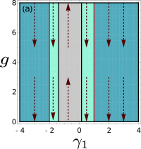
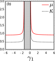
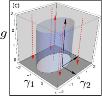
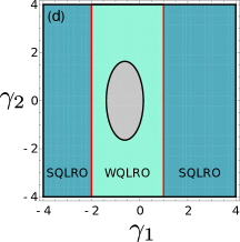
Figure 1: (a) RG flow diagram in the $g-\gamma_{1}$ plane in the achiral limit ($\gamma_{2}=0$). Arrows indicate RG flows. Flow in the stable (unstable), i.e., towards (away from) $g=0$ region are marked. (b) Variations of $\mu$ and $\kappa$ as functions of $\gamma_{1}$ in the stable region for the achiral case. (c) RG flow diagram in the space spanned by $\gamma_{1}-\gamma_{2}-g$ in the full a-KPZ equation. RG flow lines in the stable and unstable regions are shown by the arrows. (d) Phase diagram in the $\gamma_{1}-\gamma_{2}$ plane for the a-KPZ equation. The central gray region containing the origin is unstable. Regions with SQLRO and WQLRO are marked (see text).

The chiral effects ($\gamma_{2}\neq 0$) can be included in the above calculational scheme in straightforward ways: Stability of the RG flow is now determined by ${\cal A}(\gamma_{1},\gamma_{2})>0$. Flow lines having initial conditions within a narrow elliptical cylinder, containing the origin (0,0,0) and having the axis parallel to the $g$-axis, with its surface given by ${\cal A}(\gamma_{1},\gamma_{2})=0$ for any $g$, run away parallel to the $g$-axis, leaving the perturbatively accessible region. Flow lines with initial conditions falling in regions outside of this elliptical cylinder flow towards the $\gamma_{1}-\gamma_{2}$ plane with stable states. See Fig. 1(c) depicting the RG flow lines in the space spanned by $\gamma_{1}-\gamma_{2}-g$. Outside the elliptical cylinder $g(l)\sim 1/({\cal A}l)$ for large $l$, similar to its achiral analog. Inside the cylinder, $g(l)$ diverges as $l\rightarrow 1/(|{\cal A}|)$ from below. Focusing on the $\gamma_{1}-\gamma_{2}$ plane, ${\cal A}(\gamma_{1},\gamma_{2})=0$ sketches out an inner elliptical unstable region, whereas the outer region is stable; see Fig.1(d). We use the above results to find that in the stable region $\Delta\sim[\ln(L/a)]^{\mu(\gamma_{1},\gamma_{2})}$, where $\mu=1+({\cal B}-{\cal C})/{\cal A}$ is now parametrised by both $\gamma_{1},\gamma_{2}$. Similar to and quantitatively extending the achiral case, $\mu<1(>1)$ is referred to as SQLRO (WQLRO), giving positional generalised QLRO. The SQLRO and WQLRO regions are demarcated within the stable region in Fig. 1(d).

We further find that the equal-time height-difference correlator $C_{h}(r,0)\equiv\langle[h({\bf x},t)-h(0,t)]^{2}\rangle\sim\frac{D_{0}}{\nu_{0}}[\ln(r/a)]^{\mu}$, for large $r\equiv|{\bf x}|\gg a$, indicating logarithmically faster or slower rise with the separation $r$ for large $r$ Haldar et al. (2023a, b), again generalising .the well-known QLRO found in an EW surface at 2D.

Our continuously varying scaling exponents are a crucial outcome of the nonrenormalisation of $\lambda,\lambda_{1}$ and $\lambda_{2}$, rendering $\gamma_{1},\gamma_{2}$ marginal, which have been demonstrated at the one-loop order. Unlike the usual KPZ equation, Galilean invariance of the present model ensures nonrenormalisation of a combination of $\lambda,\,\lambda_{1},\,\lambda_{2}$, and not each of them individually. Thus, there is no surety that $\gamma_{1},\gamma_{2}$ should remain marginal even at higher-loop orders. We now argue that these possible higher-loop contributions, even though may exist, actually do not matter. Since we are at the critical dimension, $g(l)\sim 1/l$ for large $l$ at the one-loop order. At higher-loop orders, the Feynman diagrams will contain higher power of $g$. Hence, a general scaling solution for $g(l)$ should have the form $g(l)\sim 1/l+\sum_{n}c_{n}/l^{n},\,n>1$ is an integer. Thus, the higher-loop corrections to the one-loop solution of $g(l)$ should vanish like $1/l$ to a power greater than 1. Therefore, their integrals over $l$ from zero to infinity will be finite, so they will not change the anomalous behavior of $D$ and $\nu$. Similarly, they cannot make any divergent contribution to $\gamma_{1}(l)$ and $\gamma_{2}(l)$, even though there can be higher-loop diagrams. Therefore, our one-loop results are, in fact, asymptotically exact. This then implies that the continuous variation of the scaling exponents, making them nonuniversal, is also asymptotically exact in the long wavelength limit. See Refs. Haldar et al. (2023a, b); Sarkar and Basu (2012); Basu and Frey (2004, 2009); Bratanov et al. (2015); Mahault et al. (2018); Haldar and Basu (2022) for similar nonuniversal scaling exponents in other models.

At higher dimensions $d>2$, the chiral term with coupling $\lambda_{2}$ cannot exist. The other two achiral nonlinear terms in Eq. (15) are present at $d>2$. The RG recursion relations for $d>2$ can be obtained from the Feynman diagrams given in SM with $\gamma_{2}=0$. Using a $d=2+\epsilon$ expansion as in the KPZ equation Tang et al. (1990), we find at the one-loop order or to the lowest order in $\epsilon$

$$\frac{dg}{dl}=-\epsilon g-{\cal\tilde{A}}(\gamma_{1})g^{2}.$$ (8)

Parameter $\gamma_{1}$ remains marginal at the lowest order. Therefore, if ${\cal\tilde{A}}(\gamma_{1})>0$, $g(l)$ flows to zero rapidly, with $g(l)\sim g(0)\exp(-\epsilon\,l)$ in the long wavelength limit; $g^{*}=0$ is the only FP that is globally stable. This renders the nonlinearities irrelevant in the RG sense. Therefore, scaling in the long wavelength limit is identical to that in the EW equation: $z=2,\,\chi=(2-d)/2$. Furthermore, $d=2$ is then the upper critical dimension. On the other hand, if ${\cal\tilde{A}}(\gamma_{1})<0$, $g(l)$ has three FPs: $g^{*}_{c}=-\epsilon/{\cal\tilde{A}}(\gamma_{1})$, an unstable FP, parametrised by $\gamma_{1}$ and separating possibly two stable FPs, one being at $g^{*}=0$ Gaussian FP with EW scaling for that $d$, and another putative perturbatively inaccessible FP, corresponding presumably to an algebraically rough phase. This gives, with 2D as the lower critical dimension, a roughening transition at $d>2$, very similar to the KPZ equation at $d>2$, but with one caveat. At this unstable FP, using (3) and (4), to ${\cal O}(\epsilon)$ $z=2+\epsilon\frac{{\cal\tilde{C}}(\gamma_{1})}{{\cal\tilde{A}}(\gamma_{1})},\,\,\chi=-\epsilon\frac{{\cal\tilde{C}}(\gamma_{1})}{{\cal\tilde{A}}(\gamma_{1})}$, depend explicitly on $\gamma_{1}$ and deviate from their linear theory (or EW equation) values already at ${\cal O}(\epsilon)$. This is in contrast to the KPZ equation at $d>2$, where $z$ and $\chi$ at the unstable FP are at least ${\cal O}(\epsilon^{2})$ Tang et al. (1990). In fact, application of the Cole-Hopf transformation shows that $z=2,\,\chi=0$ at the unstable FP of the KPZ equation at $d>2$ Janssen et al. (1999).

In the parameter space where ${\cal\tilde{A}}(\gamma_{1})<0$, solution of ${\cal\tilde{C}}(\gamma_{1})=0$ gives the red dashed lines $\gamma_{1}=\gamma^{-},\gamma^{{\dagger}}$ where, $\gamma^{{\dagger}}=0$ and $\gamma^{-}=-1.25$; see Fig. 2(a) for variation of $z$ and $\chi$ with $\gamma_{1}$ for a fixed $\epsilon$. Green strips correspond to ${\cal\tilde{C}}(\gamma_{1})>0$ where $\chi>0$ and $z<2$; ${\cal\tilde{C}}(\gamma_{1})<0$ is the blue region where, $\chi<0$ and $z>2$. For a given $\epsilon$, maximum value of $z$ and minimum value of $\chi$ are $z_{\text{max}}=2+0.292\epsilon$ and $\chi_{\text{min}}=-0.292\epsilon$ at $\gamma_{1}=-0.651$, such that the dynamics is slowest and the surface is smoothest at the unstable FP. Since $\chi_{\text{min}}>\chi_{\text{EW}}=-\epsilon/2$, an a-KPZ surface at the unstable FP is always rougher than an EW surface.

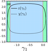
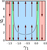
Figure 2: (a) Variation of $z$ and $\chi$ with $\gamma_{1}$ on the fixed line $g_{c}^{*}=-1/{\cal\tilde{A}}(\gamma_{1})$ for $\epsilon=1$, (b) RG flow diagram in the $g-\gamma_{1}$ plane for $d>2$. The black dashed line is the fixed line $g_{c}^{*}=-1/{\cal\tilde{A}}(\gamma_{1})$ for $\epsilon=1$, bounded by lines $\gamma_{1}=\gamma_{-},\gamma_{+}$ (blue dashed lines). Stable (unstable) flow lines are the arrows pointing towards (away from) $g=0$ (see text).

In the $g-\gamma_{1}$ plane, $g_{c}^{*}=-\epsilon/{\cal\tilde{A}}(\gamma_{1})$ is a fixed line, such that RG flow lines with initial $g$ values above the line flows to perturbatively inaccessible FP, see Fig. 2(b). And for systems with initial $g$ values lying below the line, the RG flow lines run parallel to the $g$-axis towards Gaussian FP, corresponding to the smooth phase belonging to the EW class. This behaviour holds within a range $\gamma_{-}>\gamma_{1}>\gamma_{+}$. As $\gamma_{1}\rightarrow\gamma_{+},\,\gamma_{-}$, ${\cal\tilde{A}}(\gamma_{1})$ vanishes and $g_{c}^{*}$ diverges. As soon as $\gamma_{1}$ exceeds $\gamma_{+}$ or falls short of $\gamma_{-}$, $g_{c}^{*}$ no longer exists with the roughening transition disappearing. RG flow lines starting from any initial condition with $\gamma_{1}>\gamma_{+}$ or $\gamma_{1}<\gamma_{-}$ (red region) where ${\cal\tilde{A}}(\gamma_{1})>0$, flow to $g^{*}=0$ ensuing scaling belonging to the EW class. Thus the roughening transition of the KPZ equation is entirely suppressed by the nonlocal nonlinear term.

In summary, we have proposed and studied an “active KPZ” equation, having a surface velocity $v_{p}$ depending nonlocally on the surface gradients. Surprisingly, we find stable surfaces with positional generalised QLRO or generalised logarithmic roughness with nonuniversal exponents for wide-ranging choices of the model parameters, unlike the 2D KPZ equation. Physically, this is due to the competition between the nonlocal and local nonlinear terms and the lack of their renormalisation. At $d>2$, similar choices for the same parameters can suppress the KPZ roughening transitions, resulting into only smooth surfaces. Heuristically, a nonlocal part in $v_{p}$ means a local large fluctuation can generate a propulsion not just locally, but over large scales, which when sufficiently strong can suppress local variations in $v_{p}$ due to the local KPZ-nonlinear term. This in turn has the effect of reducing surface fluctuations. For other parameter choices, a KPZ-like perturbatively inaccessible rough phase is speculated. This may be explored by mode-coupling methods Bhattacharjee (1998). In that parameter space, the roughening transition survives at $d>2$, but with significantly different scaling properties, again with nonuniversal exponents. We hope our studies here will provide further impetus to study nonlocal effects on similar nonequilibrium surface dynamics models, e.g., the conserved KPZ Sun et al. (1989); Caballero et al. (2018) and the $|{\bf q}|$KPZ Besse et al. (2023) equations.

Acknowledgement:- A.B. thanks the SERB, DST (India) for partial financial support through the MATRICS scheme [file no.: MTR/2020/000406].

Appendix A Active KPZ equation

We first construct the appropriate equation in terms of the vector field ${\bf v}({\bf r},t)\equiv{\bm{\nabla}}h$. Field $\bf v$ has a definite physical interpretation: for an active membrane $\bf v$ is the fluctuation of the local normal to the membrane surface Chaikin and Lubensky (2000). Noting that the Burgers velocity $\bf v$ is a conserved vector field, it must follow a generic conservation law of the form

$$\frac{\partial v_{i}}{\partial t}=-\nabla_{j}J_{ij},$$ (9)

where $J_{ij}$ is the velocity current. In general $J_{ij}$ can be decomposed as the sum of a symmetric part $J_{ij}^{s}=J_{ji}^{s}$ and an antisymmetric part $J_{ij}^{a}=-J_{ji}^{a}$: $J_{ij}=J_{ij}^{s}+J_{ij}^{a}$. Since $\bf v$ is purely irrolational, it can be expressed, via the Helmholtz theorem Bladel (1958); Koenigsberger (1906), solely in terms of its divergence, i.e., ${\bm{\nabla}}\cdot{\bf v}\equiv{\cal D}$, which follows the equation

$$\frac{\partial{\cal D}}{\partial t}=-\nabla_{i}\nabla_{j}J_{ij}=-\nabla_{i}\nabla_{j}J_{ij}^{s}.$$ (10)

Thus, $J_{ij}^{a}$ plays no role in the dynamics of $\cal D$ and hence of $\bf v$. Without any loss of generality, we then set $J_{ij}^{a}=0$. We further express $J_{ij}=J_{ij}^{s}$ as

$$J_{ij}=\frac{1}{2}(\partial_{i}\mu_{j}+\partial_{j}\mu_{i}),$$ (11)

where ${\bm{\mu}}$ is the “chemical potential” vector, which in general can have irrolational and solenoidal parts. The latter part does not contribute to the dynamics of ${\cal D}$ and hence of $\bf v$, and hence can be set to zero, leaving $\bm{\mu}$ purely irrolational. In that case,

$$\frac{\partial{\bf v}}{\partial t}=-\nabla^{2}{\bm{\mu}}.$$ (12)

The Burgers equation is given by

$$\frac{\partial v_{i}}{\partial t}=\nu\nabla^{2}v_{i}+\frac{\lambda}{2}\nabla_{i}v^{2}+f_{i}.$$ (13)

Therefore, in the linearised Burgers equation ($\lambda=0$), ${\bm{\mu}}=-\nu{\bf v}$, a local quantity, whereas for the Burgers equation ${\bm{\mu}}=-\frac{\lambda}{2}\nabla^{-2}{\bm{\nabla}}{v^{2}}$, a nonlocal quantity.

Now consistent with the conservation law form of the Burgers equation, $\mu_{i}$ can be generalised from its form for the Burgers equation: It also admits, at the same order, a second contribution of the form $\sim\nabla_{j}(v_{i}v_{j})/\nabla^{2}$. Indeed, including this term the most general equation of $\bf v$ retaining only up to the lowest order in nonlinearities and spatial gradients that now includes a chiral contribution is of the form

$$\frac{\partial{v_{i}}}{\partial t}=\nu\nabla^{2}{v_{i}}+\frac{\lambda}{2}{\nabla_{i}}v^{2}+\lambda_{1}\nabla_{j}(v_{i}v_{j})+\lambda_{2}\nabla_{j}e_{jm}(v_{i}v_{m})+f_{i}.$$ (14)

Both the additional nonlinear terms are nonlocal contributions to $\mu$. Equation (14) reduces to the well-known Burgers equation Forster et al. (1977) when $\lambda_{1}=0=\lambda_{2}$. Further, the tensor $e_{ij}$ is the 2D totally antisymmetric matrix, with $e_{11}=0=e_{22}$ and $e_{12}=1=-e_{21}$. Thus, the $\lambda_{2}$-term in Eq. (14) is the chiral contribution. Now, further demanding that ${\bf v}$ is fully irrotational with ${\bf v}={\bm{\nabla}}h$, the “superfluid velocity” of an XY model, or the deviation of the local normal of an interface in the Monge gauge Nelson et al. (1989), we obtain,

$$\frac{\partial h}{\partial t}= \nu\nabla^{2}h+\frac{\lambda}{2}(\bm{\nabla}h)^{2}+\lambda_{1}Q_{ij}({\bf r})(\nabla_{i}h\nabla_{j}h)$$ (15)

$$+\lambda_{2}Q_{ij}({\bf r})e_{jm}(\nabla_{i}h\nabla_{m}h)+\eta,$$

where formally $Q_{ij}=\nabla_{i}\nabla_{j}/\nabla^{2}$ and is to be understood in terms of its Fourier transform.

Appendix B Galilean invariance

Under the transformation $x_{i}^{\prime}\rightarrow x_{i}-(\lambda+2\lambda_{1})c_{i}t-\lambda_{2}e_{ij}c_{j}t$ and $t^{\prime}\rightarrow t$, where $i$ and $j$ can take values $1$ or $2$ we have,

$$\frac{\partial}{\partial t^{\prime}}\rightarrow\frac{\partial}{\partial t}+(\lambda+2\lambda_{1})\textbf{c}\cdot\bm{\nabla}-\lambda_{2}e_{ij}c_{i}\frac{\partial}{\partial x_{j}},$$ (16)

$$\bm{\nabla}^{\prime}\rightarrow\bm{\nabla}.$$ (17)

Using these we show below that if the height function $h({\bf x},t)$ transforms as $h^{\prime}({\bf x}^{\prime},t^{\prime})\rightarrow h({\bf x},t)+\textbf{c}\cdot\textbf{x}$, then Eq. (15) is invariant. Considering RHS of Eq. (15), the first term transforms as,

$$\nu\nabla^{\prime 2}h^{\prime}\rightarrow\nu\nabla^{2}h.$$ (18)

Second term transforms as,

$$\frac{\lambda}{2}(\bm{\nabla}^{\prime}h^{\prime})^{2}\rightarrow\frac{\lambda}{2}(\bm{\nabla}h)^{2}+\lambda\bm{\nabla}h\cdot\textbf{c}+\frac{\lambda}{2}c^{2}.$$ (19)

Third term transforms as,

$$\lambda_{1}\frac{\nabla^{\prime}_{i}\nabla^{\prime}_{j}}{\nabla^{\prime 2}}(\nabla^{\prime}_{i}h^{\prime}\nabla^{\prime}_{j}h^{\prime})\rightarrow\lambda_{1}\frac{\nabla_{i}\nabla_{j}}{\nabla^{2}}(\nabla_{i}h\nabla_{j}h)+2\lambda_{1}\textbf{c}\cdot\bm{\nabla}h.$$ (20)

Chiral term transforms as,

$$\lambda_{2}\frac{\nabla^{\prime}_{i}\nabla^{\prime}_{j}}{\nabla^{\prime 2}}e_{jm}(\nabla^{\prime}_{i}h^{\prime}\nabla^{\prime}_{m}h^{\prime})\rightarrow \lambda_{2}\frac{\nabla_{i}\nabla_{j}}{\nabla^{2}}e_{jm}(\nabla_{i}h\nabla_{m}h)$$

$$-\lambda_{2}e_{ij}c_{i}\frac{\partial h}{\partial x_{j}}.$$ (21)

Noise term remains invariant under this transformation. Thus after the transformation extra terms in RHS are

$$\lambda\bm{\nabla}h\cdot\textbf{c}+\frac{\lambda}{2}c^{2}+2\lambda_{1}\textbf{c}\cdot\bm{\nabla}h-\lambda_{2}e_{ij}c_{i}\frac{\partial h}{\partial x_{j}}.$$ (22)

Similarly LHS of Eq. (15) transforms as,

$$\frac{\partial h^{\prime}}{\partial t^{\prime}}\rightarrow\frac{\partial h}{\partial t}+(\lambda+2\lambda_{1})\textbf{c}\cdot\bm{\nabla}h-\lambda_{2}e_{ij}c_{i}\frac{\partial h}{\partial x_{j}}+(\lambda+2\lambda_{1})c^{2}.$$ (23)

Comparing Eq. (22) and Eq. (23) we see that Eq. (15) is invariant.

Appendix C Renormalisation group calculations

The dynamic renormalisation group calculation is conveniently performed in terms of a path integral over $h({\bf r},t)$ and its dynamic conjugate field $\hat{h}({\bf r},t)$ Täuber (2014); Bausch et al. (1976) that is equivalent to and constructed from Eq. (15) together with the noise variance. The generating functional corresponding to Eq. (15) is given by Bausch et al. (1976); Täuber (2014)

$$\mathcal{Z}=\int\mathcal{D}\hat{h}\mathcal{D}he^{-\mathcal{S}[\hat{h},h]},$$ (24)

where $\hat{h}$ is the dynamic conjugate field and $\mathcal{S}$ is the action functional:

$$S=-\int_{{\bf x},t}\hat{h}D\hat{h}+\int_{{\bf x},t}\hat{h}\bigg{\{}\partial_{t}h-\nu\nabla^{2}h-\frac{\lambda}{2}(\bm{\nabla}h)^{2}-\lambda_{1}\frac{\nabla_{i}\nabla_{j}}{\nabla^{2}}(\nabla_{i}h\nabla_{j}h)-\lambda_{2}\frac{\nabla_{i}\nabla_{j}}{\nabla^{2}}e_{jm}(\nabla_{i}h\nabla_{m}h)\bigg{\}}.$$ (25)

In momentum space action functional can be split into two parts. The first one is the Gaussian part $S_{1}$ and other one is the anharmonic part, containing the local ($\lambda$ term) and nonlocal ($\lambda_{1}$ and $\lambda_{2}$ terms) anharmonic terms, $S_{2}$. Where,

$$S_{1}=-\int_{{\bf k_{1}},\omega_{1}}\hat{h}(-{\bf k_{1}},-\omega_{1})D\hat{h}({\bf k_{1}},\omega_{1})+\int_{{\bf k_{1}},\omega_{1}}\hat{h}(-{\bf k_{1}},-\omega_{1})\bigl{\{}-i\omega_{1}+\nu k_{1}^{2}\bigl{\}}h({\bf k_{1}},\omega_{1})$$

$$S_{2}=\int_{{\bf k_{2}},\omega_{2}}\int_{{\bf k_{3}},\omega_{3}}\hat{h}(-{\bf k},-\omega)\Bigl{\{}\frac{\lambda}{2}{\bf k_{2}\cdot k_{3}}+\lambda_{1}\frac{k_{i}k_{j}}{k^{2}}(k_{2i}k_{3j})+\lambda_{2}\frac{k_{i}k_{j}}{k^{2}}e_{jm}(k_{2i}k_{3m})\Bigl{\}}h({\bf k_{2}},\omega_{2})h({\bf k_{3}},\omega_{3}).$$

In $S_{2}$, we defined ${\bf k=k_{2}+k_{3}}$ and $\omega=\omega_{2}+\omega_{3}$. A factor of $1/k^{2}$ in the terms with coefficients $\lambda_{1}$ and $\lambda_{2}$ indicate their nonlocal nature in real space. This form of $S_{2}$ holds in 2D; at $d>2$, we must set $\lambda_{2}=0$, since the chiral term is 2D specific. As discussed in the main text, these nonlocal terms are contributions to the surface velocity that depend nonlocally on the local surface fluctuations.

C.1 Linear theory results

We define Fourier transform by

$$a({\bf x},t)=\int_{{\bf q},\omega}a({\bf q},\omega)e^{i({\bf q\cdot x}-\omega t)},$$

where $a=h,\hat{h}$. Then from the Gaussian part of (25), the correlation functions at the harmonic order can be found:

$$\langle\hat{h}({\bf q},\omega)\hat{h}(-{\bf q},-\omega)\rangle_{0}=0$$ (26a)

$$\langle\hat{h}({\bf q},\omega)h(-{\bf q},-\omega)\rangle_{0}=\frac{1}{i\omega+\nu q^{2}}$$ (26b)

$$\langle\hat{h}(-{\bf q},-\omega)h({\bf q},\omega)\rangle_{0}=\frac{1}{-i\omega+\nu q^{2}}$$ (26c)

$$\langle h({\bf q},\omega)h(-{\bf q},-\omega)\rangle_{0}=\frac{2D}{\omega^{2}+\nu^{2}q^{4}}$$ (26d)

Figure 3: Diagramatic representation of two point functions.

Fig. 3 shows diagramatic representation of the propagators.

C.2 Corrections to $D$

There are total four Feynman one-loop diagrams which contribute to the fluctuation-corrections of $D$.

Figure 4: One-loop Feynman diagrams that contribute to the renormalisation of $D$

Fig. 4$(a)$ has a symmetry factor $2$ and contributes to the correction of $D$ as shown below,

$$\frac{2\lambda^{2}}{2!\times 4}\int_{{\bf q},\Omega}\frac{[\textbf{q}\cdot(\textbf{k}-\textbf{q})]^{2}\times 4D^{2}}{\bigl{(}\Omega^{2}+\nu^{2}q^{4}\bigl{)}\bigl{(}\Omega^{2}+\nu^{2}({\bf k-q})^{4}\bigl{)}}$$ (27)

$$=\frac{\lambda^{2}D^{2}}{4\nu^{3}}\int\frac{d^{2}q}{q^{2}}$$ (28)

Fig. 4$(b)$ has a symmetry factor $2$ and contributes to the correction of $D$ as shown below,

$$\frac{\lambda_{1}^{2}}{2!}\times 2\int_{{\bf q},\Omega}\frac{k_{i}k_{j}}{k^{2}}q_{i}q_{j}\frac{k_{m}k_{n}}{k^{2}}q_{m}q_{n}$$

$$\quad\quad\quad\quad\quad\times\frac{4D^{2}}{(\Omega-i\nu q^{2})^{2}(\Omega+i\nu q^{2})^{2}}$$ (29)

$$=\frac{\lambda_{1}^{2}D^{2}}{\nu^{3}}\times\frac{3}{8}\int\frac{d^{2}q}{q^{2}}$$ (30)

Fig. 4$(c)$ has a symmetry factor $2$ and contributes to the correction of $D$ as shown below,

$$\frac{\lambda_{2}^{2}}{2!}\times 2\int_{{\bf q},\Omega}\frac{k_{i}k_{j}}{k^{2}}e_{jm}q_{i}q_{m}\frac{k_{s}k_{t}}{k^{2}}e_{tr}q_{s}q_{r}$$

$$\quad\quad\quad\quad\quad\quad\times\frac{4D^{2}}{(\Omega-i\nu q^{2})^{2}(\Omega+i\nu q^{2})^{2}}$$ (31)

$$=\frac{\lambda_{2}^{2}D^{2}}{8\nu^{3}}\int\frac{d^{2}q}{q^{2}}$$ (32)

Fig. 4$(d)$ has a symmetry factor $2$ and contributes to the correction of $D$ as shown below,

$$\frac{\lambda\lambda_{1}}{2}\times 2\frac{k_{i}k_{j}}{k^{2}}\int_{{\bf q}}q_{i}q_{j}\times q^{2}\frac{4D^{2}}{4\nu^{3}q^{6}}$$ (33)

$$\frac{\lambda\lambda_{1}D^{2}}{2\nu^{3}}\int\frac{d^{2}q}{q^{2}}$$ (34)

Adding all these contributions, we obtain the total corrections to $D$:

$$D^{<}=D\Bigr{[}1+\Bigl{(}\frac{\lambda^{2}D}{4\nu^{3}}+\frac{3\lambda_{1}^{2}D}{8\nu^{3}}+\frac{\lambda_{2}^{2}D}{8\nu^{3}}+\frac{\lambda\lambda_{1}D}{2\nu^{3}}\Bigl{)}\int\frac{d^{2}q}{q^{2}}\Bigr{]}$$ (35)

C.3 Corrections to $\nu$

Figure 5: One-loop Feynman diagrams that contribute to the renormalisation of $\nu$

Fig. 5$(a)$ represents the one-loop contribution proportional to $\lambda^{2}$, which has a symmetry factor of $8$ and is given by

$$-\frac{\lambda^{2}}{4}\times\frac{8}{2!}\int_{{\bf q},\Omega}({\bf q}\cdot{\bf(k-q)})({\bf q\cdot k})\times\frac{2D}{\Omega^{2}+\nu^{2}q^{4}}$$

$$\quad\quad\quad\quad\quad\quad\quad\quad\quad\quad\quad\quad\quad\times\frac{1}{i\Omega+\nu({\bf k-q})^{2}}$$

$$=-2D\lambda^{2}\int_{{\bf q},\Omega}q_{i}(k-q)_{i}q_{j}k_{j}\times\frac{1}{\Omega^{2}+\nu^{2}q^{4}}$$

$$\quad\quad\quad\quad\quad\quad\quad\quad\quad\quad\quad\quad\quad\times\frac{-i}{\Omega-i\nu({\bf k-q})^{2}}$$

After doing the $\Omega$ integral above result becomes,

$$-\frac{2D\lambda^{2}}{2\nu^{2}}\int_{\bf q}\frac{q_{i}(k-q)_{i}q_{j}k_{j}}{q^{2}(q^{2}+({\bf k-q})^{2})}$$

Above result takes the following form after symmetrizing i.e. ${\bf q}\rightarrow({\bf q+\frac{k}{2}})$,

$$-\frac{\lambda^{2}D}{\nu^{2}}\int_{\bf q}\frac{(q+\frac{k}{2})_{i}(\frac{k}{2}-q)_{i}(q+\frac{k}{2})_{j}k_{j}}{({\bf q+\frac{k}{2}})^{2}\bigl{\{}{\bf(q+\frac{k}{2})}^{2}+({\bf\frac{k}{2}-q)}^{2}\bigl{\}}}$$

$$=\frac{\lambda^{2}D}{4\nu^{2}}\int_{\bf q}\frac{q^{2}q_{j}k_{j}+q^{2}k^{2}}{{\bf(q+\frac{k}{2})}^{2}(q^{2}+\frac{k^{2}}{4})}.$$

This then consists of two parts, coming from the two terms of the above integral. Since correction to $\nu$ is of the order of $k^{2}$, the first term in the numerator of the above integral requires binomial expansion of the denominator. After expanding for small $k$, the first term of the above integral becomes

$$-\frac{\lambda^{2}D}{2\nu^{2}}k^{2}\times\frac{1}{d}\int\frac{d^{d}q}{q^{2}}.$$

This may be evaluated by using the well-known relation Yakhot and Orzag (1986)

$$k_{i}k_{j}\int d^{d}qf(q^{2})q_{i}q_{j}=k_{i}k_{j}\times\frac{[\delta_{ij}]}{d}\int d^{d}qf(q^{2})q^{2},$$ (36)

where $f(q^{2})$ is a function of $q^{2}$. The second term of the above integral becomes contributes

$$\frac{\lambda^{2}D}{4\nu^{2}}k^{2}\times\int\frac{d^{d}q}{q^{2}}$$

to the correction to $\nu$. Adding above two results we get the total corrections to $\nu$ at ${\cal O}(\lambda)^{2}$. In 2D this takes following form

$$\frac{\lambda^{2}D}{4\nu^{2}}\frac{(d-2)}{d}k^{2}\int\frac{d^{2}q}{q^{2}}$$ (37)

Fig. 5$(b)$ has symmetry factor $8$ and represents the one-loop contribution proportional to $\lambda_{1}^{2}$ to $\nu$. This reads

$$-\frac{\lambda_{1}^{2}}{2!}\times 8\int_{{\bf q},\Omega}\frac{k_{i}k_{j}}{k^{2}}(q_{i}(k-q)_{j})\frac{q_{m}q_{n}}{q^{2}}k_{m}(k-q)_{n}$$

$$\quad\times\frac{2D}{\Omega^{2}+\nu^{2}({\bf k-q})^{4}}\times\frac{1}{-i\Omega+\nu q^{2}}$$

After doing the $\Omega$-integral above equation becomes,

$$-\frac{8\lambda_{1}^{2}}{2!}\times\frac{2D}{2\nu^{2}}\int_{\bf q}\frac{k_{i}k_{j}}{k^{2}}q_{i}(k-q)_{j}\frac{q_{m}q_{n}}{q^{2}}k_{m}(k-q)_{n}$$

$$\quad\quad\quad\quad\quad\quad\quad\quad\quad\times\frac{1}{({\bf k-q})^{2}\bigl{(}q^{2}+({\bf k-q})^{2}\bigl{)}}$$

Again we shift ${\bf q}\rightarrow({\bf q+\frac{k}{2}})$ to obtain

$$-\frac{4\lambda_{1}^{2}D}{\nu^{2}}\frac{k_{i}k_{j}k_{m}}{k^{2}}\int_{\bf q}\frac{(q+\frac{k}{2})_{i}(\frac{k}{2}-q)_{j}(q+\frac{k}{2})_{m}}{({\bf q+\frac{k}{2}})^{2}({\bf\frac{k}{2}-q})^{2}(2q^{2}+\frac{k^{2}}{2})}$$

$$\quad\quad\quad\quad\quad\quad\quad\times\frac{(q+\frac{k}{2})_{n}(\frac{k}{2}-q)_{n}}{({\bf q+\frac{k}{2}})^{2}({\bf\frac{k}{2}-q})^{2}(2q^{2}+\frac{k^{2}}{2})}$$

Since we are interested in the corrections to $\nu k^{2}$, it suffices to retain the ${\cal O}(k^{0})$ and ${\cal O}(k^{1})$ parts in the numerator, giving

$$\frac{4\lambda_{1}^{2}D}{\nu^{2}}\frac{k_{i}k_{j}k_{m}}{k^{2}}\int_{\bf q}\frac{(q_{i}q_{m}\frac{k_{j}}{2}-q_{j}q_{m}\frac{k_{i}}{2}-q_{i}q_{j}q_{m}-q_{i}q_{j}\frac{k_{m}}{2})q^{2}}{({\bf q+\frac{k}{2}})^{2}({\bf\frac{k}{2}-q})^{2}(2q^{2}+\frac{k^{2}}{2})}.$$

First two terms in the numerator of the above integral vanish as, $k_{i}k_{j}$ is symmetric but $q_{m}(q_{i}\frac{k_{j}}{2}-q_{j}\frac{k_{i}}{2})$ is antisymmetric under the interchange of $i,j$. Third term of the integrand can be expanded for small $k$, which then takes the following form $-q_{i}q_{j}q_{m}({\bf k\cdot q}-{\bf k\cdot q})$ and vanishes identically. Only fourth term contributes and can be evaluated using the identity (36). Thus above integral reduces to

$$-\frac{\lambda_{1}^{2}D}{2\nu^{2}}k^{2}\int\frac{d^{2}q}{q^{2}}.$$ (38)

Fig. 5$(c)$ has a symmetry factor $4$ and represents one of the contributions proportional to $\lambda_{1}\lambda$ where the external leg with $\hat{h}$ is from the vertex $\lambda_{1}$. This contribution is

$$- \frac{\lambda_{1}\lambda}{2}\times 4\times\frac{k_{i}k_{j}}{k^{2}}\int_{{\bf q},\Omega}q_{i}(k-q)_{j}({\bf q\cdot k})$$

$$\quad\times\frac{2D}{\Omega^{2}+\nu^{2}q^{4}}\times\frac{1}{-i\Omega+\nu({\bf k-q})^{2}}$$

After doing the $\Omega$ integral above integral becomes,

$$- 2\lambda\lambda_{1}\frac{k_{i}k_{j}k_{m}}{k^{2}}\int_{\bf q}q_{i}(k-q)_{j}q_{m}\times\frac{2D}{2\nu^{2}q^{2}\bigl{(}q^{2}+({\bf k-q})^{2}\bigl{)}}$$

After shifting ${\bf q}\rightarrow({\bf q+\frac{k}{2}})$ above result becomes,

$$-\frac{2\lambda\lambda_{1}D}{\nu^{2}}\frac{k_{i}k_{j}k_{m}}{k^{2}}\int_{\bf q}\frac{(q+\frac{k}{2})_{i}(\frac{k}{2}-q)_{j}(q+\frac{k}{2})_{m}}{({\bf q+\frac{k}{2}})^{2}(2q^{2}+\frac{k^{2}}{2})}$$

$$=-\frac{2\lambda\lambda_{1}D}{\nu^{2}}\frac{k_{i}k_{j}k_{m}}{k^{2}}\int_{\bf q}\frac{q_{i}(q_{m}\frac{k_{j}}{2}-q_{j}\frac{k_{m}}{2})-\frac{k_{i}}{2}q_{j}q_{m}-q_{i}q_{j}q_{m}}{({\bf q+\frac{k}{2}})^{2}(2q^{2}+\frac{k^{2}}{2})}$$

The first term in the numerator of the above integral vanish as $k_{j}k_{m}$ is symmetric but $q_{i}(q_{m}\frac{k_{j}}{2}-q_{j}\frac{k_{m}}{2})$ is antisymmetric under the interchange of $j,m$. We evaluate the third term by expanding for small $k$

$$\frac{2\lambda\lambda_{1}D}{\nu^{2}}\frac{k_{i}k_{j}k_{m}}{k^{2}}\Biggr{[}\int_{\bf q}\frac{\frac{k_{i}}{2}q_{j}q_{m}}{2q^{4}}-\int_{\bf q}\frac{q_{i}q_{j}q_{m}q_{n}k_{n}}{2q^{6}}\Biggr{]}.$$

The first integral in the above line can be calculated using identity (36). The second integral can be done by using the following identity Yakhot and Orzag (1986)

$$k_{i}k_{j}k_{m}k_{n}\int d^{d}qf(q^{2})q_{i}q_{j}q_{m}q_{n}=k_{i}k_{j}k_{m}k_{n}$$

$$\times\frac{[\delta_{ij}\delta_{mn}+\delta_{im}\delta_{jn}+\delta_{in}\delta_{jm}]}{d(d+2)}\int d^{d}qf(q^{2})q^{4}.$$ (39)

Thus calculating the above integrals and substituting $d=2$ we get,

$$-\frac{\lambda\lambda_{1}D}{8\nu^{2}}k^{2}\int\frac{d^{2}q}{q^{2}}$$ (40)

Fig. 5$(d)$ has symmetry factor $4$ and represents the contribution originating from vertices $\lambda_{1}$ - $\lambda$ where external leg $\hat{h}$ is from vertex $\lambda$. The contribution is,

$$-\frac{\lambda\lambda_{1}}{2}\times 4\int_{{\bf q},\Omega}{\bf q\cdot(k-q)}\frac{(k-q)_{i}(k-q)_{j}}{(k-q)^{2}}q_{i}k_{j}$$

$$\quad\times\frac{2D}{\Omega^{2}+\nu^{2}q^{4}}\times\frac{1}{-i\Omega+\nu({\bf k-q})^{2}}$$ (41)

$$=-\frac{\lambda\lambda_{1}D}{2\nu^{2}}k^{2}\int\frac{d^{2}q}{q^{2}}.$$ (42)

Fig. 5$(e)$ has a symmetry factor $2$ and represents the contribution proportional to $\lambda_{2}^{2}$. It is given by

$$\frac{\lambda_{2}^{2}}{2!}\times 2\frac{k_{i}k_{j}}{k^{2}}e_{jm}e_{tn}\int_{{\bf q},\Omega}\Bigl{(}-q_{i}(k-q)_{m}-(k-q)_{i}q_{m}\Bigl{)}$$

$$\quad\times\frac{(k-q)_{s}(k-q)_{t}}{({\bf k-q})^{2}}\Bigl{(}q_{s}k_{n}+q_{n}k_{s}\Bigl{)}$$

$$\quad\times\frac{2D}{\Omega^{2}+\nu^{2}q^{4}}\times\frac{1}{i\Omega+\nu({\bf k-q})^{2}}$$ (43)

$$=-\frac{\lambda_{2}^{2}D}{8\nu^{2}}k^{2}\int\frac{d^{2}q}{q^{2}}$$ (44)

There are no corrections proportional to $\lambda\lambda_{2}$ or $\lambda_{1}\lambda_{2}$ due to the chiral form of the $\lambda_{2}$-term.Adding all these we find the total corrections to $\nu$:

$$\nu^{<}=\nu\Bigr{[}1+\Bigl{(}\frac{\lambda_{1}^{2}D}{2\nu^{3}}+\frac{5}{8}\frac{\lambda\lambda_{1}D}{\nu^{3}}+\frac{\lambda_{2}^{2}D}{8\nu^{3}}\Bigl{)}\int\frac{d^{2}q}{q^{2}}\Bigr{]}$$ (45)

C.4 One-loop corrections to $\lambda,\lambda_{1}$ and $\lambda_{2}$

Figure 6: Representative one-loop Feynman diagrams that can contribute to the renormalisation of $\lambda$, $\lambda_{1}$ and $\lambda_{2}$.

Fig. 6 shows representative one-loop Feynman diagrams for renormalisation of $\lambda$, $\lambda_{1}$ and $\lambda_{2}$ at the one-loop order, where $a,b,c$ can take values $0,1,2$, and $\lambda_{0}=\lambda$. There are many possible similar diagrams depending on $a,b,c$ but for a particular set of vertices (i.e for a fixed values of $a,b,c$) there exist two diagrams that may contribute to the corrections of any of $\lambda,\lambda_{1},\lambda_{2}$ as shown in Fig. 6. When ($a=b=c=1$) then Fig. 6$(a)$ has symmetry factor $24$ and contributes following,

$$\frac{\lambda_{1}^{3}}{3!}\times 24\times\Bigr{[}\frac{\nabla_{i}\nabla_{j}}{\nabla^{2}}\hat{h}\nabla_{m}h\nabla_{t}h\Bigr{]}\int_{{\bf q},\Omega}q_{i}q_{j}q_{m}q_{t}$$

$$\quad\quad\quad\quad\quad\times\frac{2D}{(\Omega+i\nu q^{2})^{2}(\Omega-i\nu q^{2})^{2}}$$ (46)

$$=\frac{48\times\lambda_{1}^{3}}{3!\times 8}\times\Bigr{[}\frac{\nabla_{i}\nabla_{j}}{\nabla^{2}}\hat{h}\nabla_{m}h\nabla_{t}h\Bigr{]}\frac{2D}{8\nu^{3}}\int\frac{d^{2}q}{q^{2}}$$

$$\quad\quad\quad\quad\quad\times\Bigr{[}\delta_{ij}\delta_{mt}+\delta_{im}\delta_{jt}+\delta_{it}\delta_{jm}\Bigr{]}$$ (47)

Similarly for ($a=b=c=1$) Fig. 6$(b)$ has symmetry factor $48$ and contributes following,

$$\frac{48\lambda_{1}^{3}}{3!}\times\Bigr{[}\frac{\nabla_{i}\nabla_{j}}{\nabla^{2}}\hat{h}\nabla_{m}h\nabla_{t}h\Bigr{]}\int_{{\bf q},\Omega}q_{i}q_{j}q_{m}q_{t}$$

$$\quad\quad\quad\quad\quad\times\frac{2D}{(\Omega^{2}+\nu^{2}q^{4})(\Omega+i\nu q^{2})^{2}}$$ (48)

$$=-\frac{48\times\lambda_{1}^{3}}{3!\times 8}\times\Bigr{[}\frac{\nabla_{i}\nabla_{j}}{\nabla^{2}}\hat{h}\nabla_{m}h\nabla_{t}h\Bigr{]}\frac{2D}{8\nu^{3}}\int\frac{d^{2}q}{q^{2}}$$

$$\quad\quad\quad\quad\quad\times\Bigr{[}\delta_{ij}\delta_{mt}+\delta_{im}\delta_{jt}+\delta_{it}\delta_{jm}\Bigr{]}$$ (49)

We can see that Eq. (49) is exactly same as Eq. (47) but with a negative sign. They cancel each other contributing nothing to the corrections of $\lambda,\lambda_{1}$ and $\lambda_{2}$. In fact, for any combination of $a,b$ and $c$ there exist diagrams like Fig. 6$(a)$ and Fig. 6$(b)$ added up to zero contributing nothing to $\lambda,\lambda_{1}$ and $\lambda_{2}$.. This shows that there are no relevant corrections to $\lambda,\lambda_{1}$ and $\lambda_{2}$ at the one-loop order.

C.5 RG flow equations and scaling

After averaging over fields with higher momentum new action contains fields with upper cut off momentum $\frac{\Lambda}{b}$. Since we want to describe the same system with new action, so we have to rescale the space, time and fields so the upper cutoff momentum becomes $\Lambda$. Rescaling of space and time give ${\bf q}\to{\bf q}^{\prime}=b{\bf q}\implies x^{\prime}=\frac{x}{b}$ and $\omega\to\omega^{\prime}=b^{z}\omega\implies t^{\prime}=\frac{t}{b^{z}}$. Furthermore, rescaling of the fields $h$ and $\hat{h}$ give

$$h^{<}({\bf q},\omega)=\xi h({\bf q}^{\prime},\omega^{\prime})$$

$$\hat{h}^{<}({\bf q},\omega)=\hat{\xi}\hat{h}({\bf q}^{\prime},\omega^{\prime})$$

$$h^{<}(x,t)=\xi_{R}h(x^{\prime},t^{\prime}).$$

Now let $\xi_{R}=b^{\chi}$, where $\chi$ is the roughness exponent of the surface. Since there is no correction to $\int_{x,t}\hat{h}\partial_{t}\,h$ we impose the condition that coefficient of $\int_{x,t}\hat{h}\partial_{t}h$ remains unity under rescaling. Using these we find

$$D^{\prime}=D^{<}b^{z-d-2\chi}$$

$$\nu^{\prime}=\nu^{<}b^{z-2}$$

$$\lambda^{\prime}=\lambda b^{\chi+z-2}.$$

Here, $\lambda_{1}$ and $\lambda_{2}$ scale same as $\lambda$. Since there are no relevant one-loop corrections to $\lambda,\lambda_{1},\lambda_{2}$, $\lambda^{<}=\lambda$ etc. Furthermore,

$$D^{<}=D\Bigr{[}1+\Bigl{(}\frac{\lambda^{2}D}{4\nu^{3}}+\frac{3\lambda_{1}^{2}D}{8\nu^{3}}+\frac{\lambda_{2}^{2}D}{8\nu^{3}}+\frac{\lambda\lambda_{1}D}{2\nu^{3}}\Bigl{)}\int_{\frac{\Lambda}{b}}^{\Lambda}\frac{d^{2}q}{q^{2}}\Bigr{]}$$

and

$$\nu^{<}=\nu\Bigr{[}1+\Bigl{(}\frac{\lambda_{1}^{2}D}{2\nu^{3}}+\frac{5}{8}\frac{\lambda\lambda_{1}D}{\nu^{3}}+\frac{\lambda_{2}^{2}D}{8\nu^{3}}\Bigl{)}\int_{\frac{\Lambda}{b}}^{\Lambda}\frac{d^{2}q}{q^{2}}\Bigr{]}$$

. We set $b=e^{\delta l}\approx 1+\delta l$ and define dimensionless coupling constants by $g=\frac{\lambda^{2}D}{\nu^{3}}\frac{1}{2\pi}$,$\gamma_{1}=\frac{\lambda_{1}}{\lambda}$ and $\gamma_{2}=\frac{\lambda_{2}}{\lambda}$ to obtain the RG flow equations in the main text.

In dimensions greater than 2 (where $\gamma_{2}=0$), we set $d=2+\epsilon$ with $\epsilon>0$. We aim to determine the fixed point and the corresponding scaling exponents accurately up to $O(\epsilon)$ only. To achieve this, it suffices to substitute $d=2$ in the one-loop integrals. For example, in a general dimension where $d>2$, the RG flow equation governing the parameter $g$ is expressed as follows:

$$\frac{dg}{dl}= g\Biggr{[}2-d+g\biggl{\{}\frac{1}{4}+\frac{3}{d(d+2)}\gamma_{1}^{2}+\frac{\gamma_{1}}{d}-\frac{3}{4}\frac{2-d}{d}-\frac{3}{d}\gamma_{1}^{2}$$

$$-\frac{3\gamma_{1}}{d(d+2)}\biggl{(}3-\frac{d+2}{2}+\frac{d(d+2)}{2}\biggl{)}\biggl{\}}\Biggr{]}$$

Upon setting $d=2+\epsilon$, and considering that $g\sim{\cal O}(\epsilon)$ at the fixed point, we substitute $d=2$ selectively in the contributions coming from the one-loop integral terms containing $d$ inside the curly bracket. This yields the simplified form of the RG flow equation:

$$\frac{dg}{dl}=-\epsilon g-{\cal\tilde{A}}(\gamma_{1})g^{2}.$$

Consequently, this produces $g$ correctly to ${\cal O}(\epsilon)$; see, e.g., Ref. Barabási and Stanley (1995).

Appendix D Correlation function

Following Refs. Haldar et al. (2023a, b); Mukherjee and Basu (2022a), we now calculate the renormalised correlation functions of $h({\bf x})$, defined as

$$C_{h}^{R}(r)\equiv\langle[h({\bf x})-h({\bf x^{\prime}})]^{2}\rangle_{R},$$ (50)

where $R$ refers to a renormalised quantity. We start from

$$\langle h({\bf k})h({\bf-k})\rangle_{R}\approx\frac{D_{0}}{\nu_{0}k^{2}[\ln(\Lambda/k)]^{1-\mu}},$$ (51)

Expression (51) is no longer valid over the wavevector range from 0 to $\Lambda$, rather it is valid between 0 and $\tilde{\Lambda}\ll\Lambda$. We then obtain,

$$C_{h}(r)\approx\int_{0}^{\tilde{\Lambda}}\frac{d^{2}k}{(2\pi)^{2}}\left[1-\exp i{\bf k}\cdot({\bf x-x}^{\prime})\right]\frac{D_{0}}{\nu_{0}k^{2}[\ln(\Lambda/k)]^{1-\mu}}.$$ (52)

Integrating over the angular variable, we get

$$C_{h}(r) \approx \int_{0}^{\tilde{\Lambda}}\frac{dq\,D_{0}}{\nu_{0}q[\ln(\Lambda/q)]^{1-\mu}}\left[\frac{1}{2\pi}\int_{0}^{2\pi}d\theta(1-e^{iqr\cos\theta}\right]$$ (53)

$$= \int_{0}^{\tilde{\Lambda}}\frac{dq\,D_{0}}{\nu_{0}q[\ln(\Lambda/q)]^{1-\mu}}\left[1-J_{0}(qr)\right]$$

$$= \int_{0}^{\tilde{\Lambda}r}\frac{du\,D_{0}[1-J_{0}(u)]}{\nu_{0}u|\ln(\frac{r\Lambda}{u})|^{1-\mu}},$$

where $J_{0}(u)$ is the Bessel function of order zero. Then

$$C_{h}(r)=\int_{0}^{1}\frac{du\,D_{0}[1-J_{0}(u)]}{\nu_{0}u[-\ln u+\ln(1/y)]^{1-\mu}}+\int_{1}^{\tilde{\Lambda}r}\frac{du\,D_{0}}{\nu_{0}u[-\ln u+\ln(\Lambda r)]^{1-\mu}}-\int_{1}^{\tilde{\Lambda}r}\frac{du\,D_{0}J_{0}(u)}{\nu_{0}u[-\ln u+\ln(\Lambda r)]^{1-\mu}}.$$ (54)

The first and the third terms on the rhs of (54) are finite. Since $u_{max}=\tilde{\Lambda}r\ll\Lambda r$, the second contribution on the right may be integrated with the substitution $u=\exp(z)$ giving

$$\int_{1}^{\tilde{\Lambda}\,r}\frac{du}{u[\ln(\Lambda\,r)]^{1-\mu}}=\mu\frac{\ln(\Lambda r)+\ln(\tilde{\Lambda}/\Lambda)}{\ln(\Lambda r)}[\ln(\Lambda r)]^{\mu}\approx\mu[\ln(\Lambda\,r)]^{\mu}$$ (55)

in the limit of large $r$. We thus find $C_{h}(r)\approx\mu\frac{D_{0}}{\nu_{0}}|\ln(\Lambda\,r)|^{\mu}$ in the limit of large $r$, with the remaining contributions on the right hand side of (54) being finite or subleading for large $r$.

References

Kardar et al. (1986)M. Kardar, G. Parisi, and Yi-C. Zhang, “Dynamic scaling of growing
interfaces,” Phys. Rev. Lett. 56, 889 (1986).
Barabási and Stanley (1995)A-L Barabási and Harry Eugene Stanley, Fractal
concepts in surface growth (Cambridge university
press, 1995).
Edwards and Wilkinson (1982)S. F. Edwards and D. R. Wilkinson, “The surface
statistics of a granular aggregate,” Proc. R. Soc. Lond. A 381, 17 (1982).
Tang et al. (1990)L. H. Tang, T. Nattermann, and B. M. Forrest, “Multicritical and crossover
phenomena in surface growth,” Phys. Rev. Lett. 65, 2422–2425 (1990).
Fisher et al. (1972)M. E. Fisher, S. K. Ma, and B. G. Nickel, “Critical exponents for
long-range interactions,” Phys. Rev. Lett. 29, 917–920 (1972).
Bayong et al. (1999)E. Bayong, H. T. Diep, and T. T. Truong, “Phase transition in a
general continuous ising model with long-range interactions,” J.
Appl. Phys 85, 6088–6090 (1999).
Banerjee et al. (2019a)T. Banerjee, N. Sarkar,
J. Toner, and A. Basu, “Rolled up or crumpled: Phases of asymmetric
tethered membranes,” Phys. Rev. Lett. 122, 218002 (2019a).
Banerjee et al. (2019b)T. Banerjee, N. Sarkar,
J. Toner, and A. Basu, “Statistical mechanics of asymmetric tethered
membranes: Spiral and crumpled phases,” Phys.
Rev. E 99, 053004
(2019b).
Pelcé et al. (2004)Pierre Pelcé, Jasna Brujić,
and Laurent Costier, New Visions on Form and Growth:
Fingered Growth, Dendrites, and Flames (Oxford
University Press, 2004).
Ketterl and Hagston (1999)H. Ketterl and W. E. Hagston, “Nonlocal
effects associated with shading in surface growth,” Phys.
Rev. E 59, 2707
(1999).
Santalla and Ferreira (2018)S. N. Santalla and S. C. Ferreira, “Eden model
with nonlocal growth rules and kinetic roughening in biological systems,” Phys. Rev. E 98, 022405 (2018).
Aharonov and Rothman (1996)E. Aharonov and D. H. Rothman, “Growth of
correlated pore-scale structures in sedimentary rocks: A dynamical model,” J. Geophys. Res. Solid Earth 101, 2973 (1996).
Lichtner et al. (1996)P. C. Lichtner, C. I. Steefel, and E. H. Oelkers, eds., Reactive Transport in Porous Media (De Gruyter, 1996).
Doǧu (1981)T. Doǧu, “The importance of
pore structure and diffusion in the kinetics of gas-solid non-catalytic
reactions: Reaction of calcined limestone with so2,” J. Chem. Eng. 21, 213 (1981).
Delmono and Froment (1999)B. Delmono and G.F. Froment, “Preface,” in Catalyst deactivation 1999, Studies in Surface Science and Catalysis, Vol. 126, edited by B. Delmon and G.F. Froment (Elsevier, 1999).
R. Schumer (2017)D. J. Furbish R. Schumer, A. Taloni, “Theory connecting non- local sediment transport,
earth surface roughness, and the sadler effect,” Geophysical
Research Letters 44, 2281 (2017).
Martin et al. (2021)H. S. Martin, K. A. Podolsky, and N. K. Devaraj, “Probing the
role of chirality in phospholipid membranes,” ChemBioChem 22, 3148–3157 (2021).
Lalitha et al. (2001)S. Lalitha, A. S. Kumar,
K. J. Stine, and D. F. Covey, “Chirality in membranes: First evidence
that enantioselective interactions between cholesterol and cell membrane
lipids can be a determinant of membrane physical properties,” Journal of Supramolecular Chemistry 1, 53–61 (2001).
Forster et al. (1977)D. Forster, D. R. Nelson,
and M. J. Stephen, “Large-distance and long-time
properties of a randomly stirred fluid,” Phys.
Rev. A 16, 732–749
(1977).
Chaikin and Lubensky (2000)Paul M Chaikin and Tom C Lubensky, Principles of
condensed matter physics, Vol. 1 (Cambridge university press Cambridge, 2000).
Nelson et al. (1989)David Nelson, T Piran, and Steven Weinberg, Statistical Mechanics of Membranes
and Surfaces (WORLD SCIENTIFIC, 1989).
Marchetti et al. (2013)M. C. Marchetti, J. F. Joanny, S. Ramaswamy,
T. B. Liverpool, J. Prost, M. Rao, and R. A. Simha, “Hydrodynamics of soft active matter,” Rev.
Mod. Phys. 85, 1143–1189 (2013).
Rasshofer et al. (2022)F. Rasshofer, R. Swiderski, A. Haldar,
A. Basu, and E. Frey, “Anomalous collective dynamics of
auto-chemotactic populations,” arXiv: 2209.01047 (2022).
Kolmogorov et al. (1937)A. Kolmogorov, I. Petrovskii, and N. Piscunov, “A study of the
equation of diffusion with increase in the quantity of matter, and its
application to a biological problem,” Byul. Moskovskogo Gos. Univ. 1, 1 (1937).
Meakin et al. (1986)P. Meakin, P. Ramanlal,
L. M. Sander, and R. C. Ball, “Ballistic deposition on surfaces,” Phys. Rev. A 34, 5091 (1986).
Plischke et al. (1987)M. Plischke, Z. Rácz, and D. Liu, “Time-reversal invariance and
universality of two-dimensional growth models,” Phys.
Rev. B 35, 3485
(1987).
Liu and Plischke (1988)D. Liu and M. Plischke, “Universality in two- and
three-dimensional growth and deposition models,” Phys.
Rev. B 38, 4781
(1988).
Kondev et al. (2000)J. Kondev, C. L. Henley,
and D. G. Salinas, “Nonlinear measures for
characterizing rough surface morphologies,” Phys.
Rev. E 61, 104 (2000).
Naserabadi et al. (2017)H. D. Naserabadi, A. A. Saberi, and S. Rouhani, “Roughening
transition and universality of single step growth models in
(2+1)-dimensions,” New J. Phys. 19, 063035 (2017).
Täuber (2014)Uwe C Täuber, Critical dynamics: a
field theory approach to equilibrium and non-equilibrium scaling behavior (Cambridge University Press, 2014).
Basu and Frey (2004)A. Basu and E. Frey, “Novel universality classes
of coupled driven diffusive systems,” Phys.
Rev. E 69, 015101
(2004).
Gomes-Filho et al. (2021)M.S. Gomes-Filho, A.L.A. Penna, and F.A. Oliveira, “The
kardar-parisi-zhang exponents for the 2+1 dimensions,” Results in Physics 26, 104435 (2021).
Haldar et al. (2023a)A. Haldar, A. Sarkar,
S. Chatterjee, and A. Basu, “Mobility-induced order in active
spins on a substrate,” Phys. Rev. E 108, L032101 (2023a).
Haldar et al. (2023b)A. Haldar, A. Sarkar,
S. Chatterjee, and A. Basu, “Active model on a
substrate: Density fluctuations and phase ordering,” Phys. Rev. E 108, 034114 (2023b).
Toner (2023)J. Toner, “Roughening of
two-dimensional interfaces in nonequilibrium phase-separated systems,” Phys. Rev. E 107, 044801 (2023).
Grinstein and Pelcovits (1981)G. Grinstein and R. A. Pelcovits, “Anharmonic
effects in bulk smectic liquid crystals and other “one-dimensional
solids”,” Phys. Rev. Lett. 47, 856–859 (1981).
Grinstein and Pelcovits (1982)G. Grinstein and R. A. Pelcovits, “Smectic- transition in three dimensions,” Phys. Rev. A 26, 2196–2217 (1982).
Mukherjee and Basu (2022a)S. Mukherjee and A. Basu, “Stiffening or
softening of elastic media: Anomalous elasticity near phase transitions,” Phys. Rev. E 106, L052102 (2022a).
Mukherjee and Basu (2022b)S. Mukherjee and A. Basu, “Statistical
mechanics of phase transitions in elastic media with vanishing thermal
expansion,” Phys. Rev. E 106, 054128 (2022b).
Sarkar and Basu (2012)N. Sarkar and A. Basu, “Continuous universality in
nonequilibrium relaxational dynamics of o(2) symmetric systems,” Phys. Rev. E 85, 021113 (2012).
Mahault et al. (2018)B. Mahault, X.-c. Jiang,
E. Bertin, Y.-q. Ma, A. Patelli, X.-q. Shi, and H. Chaté, “Self-propelled particles with velocity reversals and ferromagnetic
alignment: Active matter class with second-order transition to
quasi-long-range polar order,” Phys. Rev. Lett. 120, 258002 (2018).
Haldar and Basu (2022)A. Haldar and A. Basu, “Disorders can induce
continuously varying universal scaling in driven systems,” Phys. Rev. E 105, 034104 (2022).
Janssen et al. (1999)H. K. Janssen, U. C. Täuber, and E. Frey, “Exact results for
the kardar-parisi-zhang equation with spatially correlated noise,” Eur. Phys. J. B 9, 491–511 (1999).
Bhattacharjee (1998)J. K. Bhattacharjee, “Upper
critical dimension of the kardar - parisi - zhang equation,” J. Phys. A Math. Gen. 31, L93 (1998).
Sun et al. (1989)T. Sun, H. Guo, and M. Grant, “Dynamics of driven interfaces with a
conservation law,” Phys. Rev. A 40, 6763–6766 (1989).
Caballero et al. (2018)F. Caballero, C. Nardini,
F. van Wijland, and M. E. Cates, “Strong coupling in conserved surface
roughening: A new universality class?” Phys. Rev. Lett. 121, 020601 (2018).
Besse et al. (2023)M. Besse, G. Fausti,
M. E. Cates, B. Delamotte, and C. Nardini, “Interface roughening in nonequilibrium
phase-separated systems,” Phys. Rev. Lett. 130, 187102 (2023).
Bladel (1958)J. Bladel, On Helmholtz’s Theorem
in Finite Regions (Midwestern Universities
Research Association, 1958).
Koenigsberger (1906)L. Koenigsberger, Hermann von
Helmholtz (Clarendon Press, 1906).
Yakhot and Orzag (1986)V. Yakhot and S. A. Orzag, “Renormalization
group analysis of turbulence. i. basic theory, v. yakhot and s. a. orzag,” Journal of
Scientific Computing 1, 3 (1986).