Numerical analysis of the stochastic Stefan problem

Abstract

The gradient discretisation method (GDM) – a generic framework encompassing many numerical methods – is studied for a general stochastic Stefan problem with multiplicative noise. The convergence of the numerical solutions is proved by compactness method using discrete functional analysis tools, Skorohod theorem and the martingale representation theorem. The generic convergence results established in the GDM framework are applicable to a range of different numerical methods, including for example mass-lumped finite elements, but also some finite volume methods, mimetic methods, lowest-order virtual element methods, etc. Theoretical results are complemented by numerical tests based on two methods that fit in GDM framework.

Keywords: Stefan equation, stochastic PDE, numerical methods, gradient discretisation method, convergence analysis

1 Introduction

In this paper, we study the stochastic Stefan problem (SSP) with multiplicative noise of the form

$$du-\text{div}[\Lambda\nabla\zeta(u)]dt=f(\zeta(u))dW_{t}\quad\text{in}\quad\Theta_{T}:=(0,T)\times\Theta,$$

$$u(0,\cdot)=u_{0}\quad\text{in}\quad\Theta,$$

$$\zeta(u)=0\quad\text{on}\quad(0,T)\times\partial\Theta,$$

where $T>0$, $\Theta$ is an open bounded domain in $\mathbb{R}^{d}\left(d\geq 1\right)$, $\Lambda$ is a diffusion coefficient and $W$ is a $\mathcal{Q}$-Wiener process. Here $\zeta$ is a globally non-decreasing Lipschitz continuous function passing through origin and coercive, see Section 2.1 for detail.

The deterministic Stefan problem describes the behavior of phase transition during the evolution of two thermodynamical states, say solid and liquid. This problem has its name from Jožef Stefan (1835-1893) due to his research on solid-liquid phase changes in formation of ice in polar seas [22]. Deterministic moving boundary problems have been studied extensively in the second half of the past century, see [18] and references therein. Numerical analysis of the problem is developed in [19, 15, 10] and a huge bibliography can be found in [23]. Convergence of variety of gradient schemes (GS) to approximate its solution is provided in [11] and [6, Chapter 6].

In the past decade, several authors have started investigating stochastic perturbation of the classical Stefan problem. There are numerous examples of applications, such as climate models, diffusion of lithium-ions in lithium-ion batteries, modeling steam chambers for petroleum extraction and oxygen diffusion in an absorbing tissue, which are described by stochastic Stefan-type problems.

A significant literature is available on proving the existence and uniqueness of SSP. In [1], a semigroup approach was employed to obtain a mild solution. Using the enthalpy function with additive noise, the two phase free boundary problem is transformed into a stochastic evolution equation of porous media type with the fixed boundary conditions. Applying a coordinate transform, [17] studied the linear SSP on one dimensional unbounded domains ($d=1$) assuming the random field Brownian in time but correlated (colored) in space. Extending these results, [16] established the existence and uniqueness of local strong solutions by using the interpolation theory. The analysis is based on the theory of mild and strong solutions proposed in [4]. A further extension of these results under Robin boundary conditions was done in [21] (in which the moving interface between the two phases might have unbounded variation).

Several works on the numerical approximation of stochastic PDEs driven by Wiener processes have been carried out, such as the heat equation, the Navier–Stokes model, the $p$-Laplace equation, etc. (see, e.g., [8, 3, 13, 12, 20, 24, 25, 26, 5]). However, to the authors’ knowledge, there is no available literature on the numerical analysis of the Stochastic Stefan problem.

This paper is primarily focused on the numerical analysis of SSP encompassing well known discrete schemes. We use a generic framework known as gradient discretisation method (GDM) to propose a numerical scheme approximating solutions of SSP. The GDM covers a large class of conforming and nonconforming schemes such as finite volume methods, Galerkin methods (including mass-lumped finite element), mixed finite element methods, hybrid high-order and virtual element methods, etc. A thorough discussion on the analysis and applications of the GDM method is given in the monograph [6]. Moreover, we prove the convergence and stability of the numerical solutions, therefore, there is no need to prove convergence for each specific method which simplifies the analysis.

Our convergence analysis technique is based on the discrete functional analysis tools, Skorokhod theorem, Kolmogorov test, and martingale representation theorem. We used the similar idea as prescribed in [8] to show the existence of a weak martingale solution to the SSP.

This paper is organised as follows: Section 2 starts with the introduction of assumptions and notations followed by the description of the GDM framework and the related gradient scheme for the SSP; two examples of methods fitting the framework are presented (the mass-lumped $\mathbb{P}_{1}$ finite element (MLP1) method and hybrid mimetic method (HMM)), and the section concludes with the statement of the main convergence result. In Section 3 we provide a priori estimates of the approximated solutions. Section 4 details the following convergence steps: (1) tightness, in appropriate spaces, of a family of random variables representing in particular the solution to the GS and their gradient, (2) almost sure convergence (up to a change of probability space) in appropriate norms, and (3) continuity of the limits of the numerical solution and of the martingale involving the Wiener process. In Section 5, the limit of the martingale part is identified, after which the main convergence result is proved. Numerical results, based on the two examples of GDs presented in Section 2, are provided in Section 6 to validate the convergence results and their bounds.

2 Gradient scheme and main results

2.1 Assumptions and notations

We first introduce the notations and assumptions that are used in the rest of the paper. Most of the time, the Lebesgue spaces we consider are those in $\Theta$, so we write $L^{r}$ instead of $L^{r}(\Theta)$. For a given $s\in[0,T]$, we set $\Theta_{s}=(0,s)\times\Theta$. Throughout this paper, we assume the following.

• $\zeta:\mathbb{R}\rightarrow\mathbb{R}$ is Lipschitz continuous with Lipschitz constant $L^{-1}_{\zeta}$. We also assume that $\zeta$ is non decreasing, satisfies $\zeta(0)=0$ and is coercive in the sense that there exists $c,d>0$ such that $\zeta(s)\geq c|s|-d$ for all $s\in\mathbb{R}$.

We set

$$\Xi(z):=\int_{0}^{z}\zeta(s)ds,\quad\forall z\in\mathbb{R}.$$

• $\Lambda:\Theta\rightarrow\mathcal{S}^{d}(\mathbb{R})$ is a symmetric measurable tensor that is uniformly elliptic and bounded, that is:

  $$\exists\;\underline{\mu},\overline{\mu}\in(0,\infty)\;\;\text{s.t.}\;\;\underline{\mu}|\xi|^{2}\leq\Lambda(x)\xi\cdot\xi\leq\overline{\mu}|\xi|^{2}\quad\forall\xi\in\mathbb{R}^{d},\;\;\text{for a.e}\;\;x\in\Theta.$$

  We will use the notation $\left\|F\right\|^{2}_{\Lambda}$ for $\left\langle\Lambda F,F\right\rangle_{L^{2}}$.

• $u_{0}:\Theta\rightarrow\mathbb{R}$ is a measurable function and satisfies

  $$\left\|\Xi(u_{0})\right\|_{L^{1}(\Theta)}+\left\|\nabla\zeta(u_{0})\right\|^{2}_{\Lambda}<+\infty.$$ (2.1)

• Let $(\Omega,\mathcal{F},\mathbb{F}=(\mathcal{F}_{t})_{t\in[0,T]},\mathbb{P})$ be a stochastic basis, that is, $(\Omega,\mathcal{F},\mathbb{P})$ is a probability space equipped with an increasing family of $\sigma$-algebras $\{\mathcal{F}_{t}\},\;t\in[0,T]$, called filtration. Assume an $\mathbb{F}$-adapted Wiener process $W=\{W(t);t\in[0,T]\}$ taking values in a separable Hilbert space $\mathcal{K}$ with covariance operator $\mathcal{Q}$ such that $Tr(\mathcal{Q})<\infty$. $W$ can be written in the form $W(t)=\sum_{k=1}^{\infty}q_{k}W_{k}(t)e_{k},$ where $\{e_{k},k\geq 1\}$ is an orthonormal basis of $\mathcal{K}$ with corresponding eigenvalues $q_{k}$ such that $\sum_{k=1}^{\infty}q^{2}_{k}<\infty$, and $\{W_{k}:k\geq 1\}$ is a family of independent $\mathbb{F}$-adapted real-valued Wiener processes.

• Let $\mathcal{L}(\mathcal{K},L^{2})$ be the Banach space of Hilbert-Schmidt operators [4, Appendix C] with norm denoted as $\left\|\cdot\right\|_{\mathcal{L}(\mathcal{K},L^{2})}$. We assume that the operator $f:L^{2}\rightarrow\mathcal{L}(\mathcal{K},L^{2})$ is continuous and that there exist $C_{1},C_{2}>0$ such that for any $w\in L^{2}$ and $\Xi(w)\in L^{1}$

  $$\left\|f(\zeta(w))\right\|^{2}_{\mathcal{L}(\mathcal{K},L^{2})}\leq C_{2}\int_{\Theta}\Xi(w)dx+C_{1}.$$ (2.2)

  
  

Throughout this article, $C$ denotes a generic constant depends on $f,T,\mathcal{Q},u_{0},\Lambda$ and $\zeta$. We will only mention any further dependencies in its subscript.

2.2 Gradient scheme

We recall here the main definitions of the Gradient Discretisation Method.

Definition 2.1.

$\mathcal{D}=(X_{\mathcal{D},0},\Pi_{\mathcal{D}},\nabla_{\mathcal{D}},\mathcal{I}_{\mathcal{D}},(t^{(n)})_{n=0,\cdots,N})$ is a space-time gradient discretisation (GD) for the homogeneous Dirichlet boundary conditions, with piecewise constant reconstruction, if the following properties hold:

1. $X_{\mathcal{D},0}$ is a finite dimensional vector space of discrete unknowns,

2. The linear map $\Pi_{\mathcal{D}}:X_{\mathcal{D},0}\rightarrow L^{\infty}$ is a piecewise constant reconstruction operator in the following sense: there exist a basis $(\mathbf{e}_{i})_{i\in B}$ of $X_{\mathcal{D},0}$ and a family of disjoint subsets $(\Theta_{i})_{i\in B}$ of $\Theta$ such that $\Pi_{\mathcal{D}}u=\sum_{i\in B}u_{i}\mathbbm{1}_{\Theta_{i}}$ for all $u=\sum_{i\in B}u_{i}\mathbf{e}_{i}\in X_{\mathcal{D},0}$, where $\mathbbm{1}_{\Theta_{i}}$ is the characteristic function of $\Theta_{i}$,

3. The linear map $\nabla_{\mathcal{D}}:X_{\mathcal{D},0}\rightarrow(L^{2})^{d}$ gives a reconstructed discrete gradient such that the mapping $v\mapsto\left\|\nabla_{\mathcal{D}}v\right\|_{L^{2}}$ is a norm on $X_{\mathcal{D},0}$,

4. $\mathcal{I}_{\mathcal{D}}:L^{2}\rightarrow X_{\mathcal{D},0}$ is an interpolation operator that is used to create, from an initial condition in $L^{2}$, a discrete vector in the space of unknowns,

5. $t^{(0)}=0<t^{(1)}<\cdots<t^{(N)}=T$ is a uniform time discretisation with a constant time step $\delta t_{\mathcal{D}}:=t^{(n+1)}-t^{(n)}$.

For any family $(v^{(n)})_{n=0,\cdots,N}\in X_{\mathcal{D},0}^{N+1}$, we defined piecewise-constant-in-time functions $\Pi_{\mathcal{D}}v:[0,T]\rightarrow L^{\infty}$, $\nabla_{\mathcal{D}}v:(0,T]\rightarrow(L^{2})^{d}$ and $d^{(n+\frac{1}{2})}_{\mathcal{D}}v\in L^{\infty}$ by: for $n=0,\cdots,N-1$, for any $t\in(t^{(n)},t^{(n+1)}]$ and for a.e. $\boldsymbol{x}\in\Theta$

$$\Pi_{\mathcal{D}}v(0,\boldsymbol{x}):=\Pi_{\mathcal{D}}v^{(0)}(\boldsymbol{x}),\quad\Pi_{\mathcal{D}}v(t,\boldsymbol{x}):=\Pi_{\mathcal{D}}v^{(n+1)}(\boldsymbol{x}),$$

$$\nabla_{\mathcal{D}}v(t,\boldsymbol{x}):=\nabla_{\mathcal{D}}v^{(n+1)}(\boldsymbol{x}),\quad d^{(n+\frac{1}{2})}_{\mathcal{D}}v(\boldsymbol{x}):=\Pi_{\mathcal{D}}v^{(n+1)}(\boldsymbol{x})-\Pi_{\mathcal{D}}v^{(n)}(\boldsymbol{x}).$$

Let $g:\mathbb{R}\rightarrow\mathbb{R}$ be such that $g(0)=0$. For $v=\sum_{i\in B}v_{i}\mathbf{e}_{i}\in X_{\mathcal{D},0}$, we set $g(v)=\sum_{i\in B}g(v_{i})\mathbf{e}_{i}\in X_{\mathcal{D},0}$. The piecewise constant feature of $\Pi_{\mathcal{D}}$ implies

$$\Pi_{\mathcal{D}}g(v)=g(\Pi_{\mathcal{D}}v)\quad\forall v\in X_{\mathcal{D},0}.$$ (2.3)

We define the filtration $(\mathcal{F}^{n}_{N})_{0\leq n\leq N}$ by:

$$\mathcal{F}^{n}_{N}:=\sigma\{W(t^{k}):0\leq k\leq n\}\qquad\forall n=0,\ldots,N.$$

Algorithm 2.1.

[Gradient Scheme (GS) for (LABEL:eq:mp)] Set $u^{(0)}:=\mathcal{I}_{\mathcal{D}}u_{0}$ and take the random variables $u(\cdot)=(u^{(n)}(\omega,\cdot))_{n=0,\cdots,N}\in X_{\mathcal{D},0}^{N+1}$ such that $u$ is adapted to the filtration $(\mathcal{F}^{n}_{N})_{0\leq n\leq N}$ and, for any $\phi\in X_{\mathcal{D},0}$ and for almost every $\omega\in\Omega$, we have, for $n=0,\cdots,N-1$,

$$\left\langle d^{(n+\frac{1}{2})}_{\mathcal{D}}u,\Pi_{\mathcal{D}}\phi\right\rangle_{L^{2}}+\delta t_{\mathcal{D}}\left\langle\Lambda\nabla_{\mathcal{D}}\zeta(u^{(n+1)}),\nabla_{\mathcal{D}}\phi\right\rangle_{L^{2}}=\left\langle f(\Pi_{\mathcal{D}}\zeta(u^{(n)}))\Delta^{(n+1)}W,\Pi_{\mathcal{D}}\phi\right\rangle_{L^{2}},$$ (2.4)

where $\Delta^{(n+1)}W=W(t^{(n+1)})-W(t^{(n)})$.

The convergence of the scheme is analysed along a sequence $(\mathcal{D}_{m})_{m\in\mathbb{N}}$ of GDs (such a sequence plays the role, in standard mesh-based schemes, of sequences of meshes with size going to zero). To establish this convergence, the sequence must satisfy a few key properties: consistency, limit-conformity and compactness.

Definition 2.2.

(Consistency) A sequence $(\mathcal{D}_{m})_{m\in\mathbb{N}}$ of space-time GDs is said to be consistent if

• for all $\phi\in H_{0}^{1}$, we have $S_{\mathcal{D}_{m}}(\phi)\rightarrow 0$ as $m\rightarrow\infty$, where

  $$S_{\mathcal{D}_{m}}(\phi):=\min_{w\in X_{\mathcal{D}_{m}}}\left(\left\|\Pi_{\mathcal{D}_{m}}w-\phi\right\|_{L^{2}}+\left\|\nabla_{\mathcal{D}_{m}}w-\nabla\phi\right\|_{L^{2}}\right),$$ (2.5)

• for all $\phi\in L^{2}$, $\Pi_{\mathcal{D}_{m}}\mathcal{I}_{\mathcal{D}_{m}}\phi\rightarrow\phi$ in $L^{2}$ as $m\rightarrow\infty$,

• $\delta t_{\mathcal{D}_{m}}\rightarrow 0$ as $m\rightarrow\infty$.

Definition 2.3.

(Limit Conformity) A sequence $(\mathcal{D}_{m})_{m\in\mathbb{N}}$ of space-time GDs is said to be limit conforming if, for all $\boldsymbol{\phi}\in H^{\text{div}}(\Theta):=\{\boldsymbol{\phi}\in(L^{2})^{d}:\text{div}\boldsymbol{\phi}\in L^{2}(\Theta)\}$, we have $W_{\mathcal{D}_{m}}(\phi)\rightarrow 0$ as $m\rightarrow\infty$, where

$$W_{\mathcal{D}_{m}}(\boldsymbol{\phi}):=\max_{v\in X_{\mathcal{D}_{m}}\setminus\{0\}}\frac{\left|\left\langle\nabla_{\mathcal{D}_{m}}v,\boldsymbol{\phi}\right\rangle_{L^{2}}+\left\langle\Pi_{\mathcal{D}_{m}}v,\text{div}\boldsymbol{\phi}\right\rangle_{L^{2}}\right|}{\left\|\nabla_{\mathcal{D}_{m}}v\right\|_{L^{2}}}.$$

Definition 2.4.

(Compactness) A sequence of $(\mathcal{D}_{m})_{m\in\mathbb{N}}$ of space-time GDs is said to be compact if

$$\lim\limits_{\xi\rightarrow 0}\sup\limits_{m\in\mathbb{N}}T_{\mathcal{D}_{m}}(\xi)=0,$$

where, extending $\Pi_{\mathcal{D}_{m}}v$ by $0$ outside $\Theta$,

$$T_{\mathcal{D}_{m}}(\xi):=\max_{v\in X_{\mathcal{D}_{m}}\setminus\{0\}}\frac{\left\|\Pi_{\mathcal{D}_{m}}v(\cdot+\xi)-\Pi_{\mathcal{D}_{m}}v\right\|_{L^{2}(\mathbb{R}^{d})}}{\left\|\nabla_{\mathcal{D}_{m}}v\right\|_{L^{2}}},\quad\forall\xi\in\mathbb{R}^{d}.$$

A limit conforming or compact sequence of GDs also satisfy the following important property, which states a (uniform) discrete Poincaré inequality.

Lemma 2.1.

(Coercivity of sequence of GDs) If a sequence $(\mathcal{D}_{m})_{m\in\mathbb{N}}$ of space-time GDs is compact or limit conforming then it is coercive: there exist a constant $\rho$ such that

$$\max_{v\in X_{\mathcal{D}_{m}}\setminus\{0\}}\frac{\left\|\Pi_{\mathcal{D}_{m}}v\right\|_{L^{2}}}{\left\|\nabla_{\mathcal{D}_{m}}v\right\|_{L^{2}}}\leq\rho\quad\forall m\in\mathbb{N}.$$ (2.6)

2.3 Examples of gradient discretisations

We present here two examples of GDs: the mass-lumped $\mathcal{P}^{1}$ (MLP1) finite elements, and the hybrid mimetic mixed method (HMM). Both of them are known to satisfy the properties above under standard mesh regularity assumptions [6].

We first specify the Gradient discretisation 2.1 for MLP1. This GD is based on a conforming triangulation of the domain $\Omega$. Let $X_{\mathcal{D},0}=\{v=(v_{s})_{s\in\mathcal{V}}:v_{s}\in\mathbb{R},\;v_{s}=0\;\text{if}\;s\in\partial\Theta\}$, where $\mathcal{V}$ is the set of all vertices. To define the reconstruction operator $\Pi_{\mathcal{D}}$, we construct a dual mesh $(\Theta_{s})_{s\in\mathcal{V}}$, which can for example be defined by setting $\Theta_{s}$ as the polygon obtained by linking the centers of the edges and cells having $s$ as a vertex (see [6, Section 8.4] for more detail). We then define the piecewise constant reconstruction on this dual mesh $\Pi_{\mathcal{D}}$ by:

$$\forall u\in X_{\mathcal{D},0},\quad\forall s\in\mathcal{V},\quad\Pi_{\mathcal{D}}u=u_{s}\;\;\text{on}\;\;\Theta_{s}.$$

Further, the reconstructed gradient $\nabla_{\mathcal{D}}$ is the gradient of piecewise linear function based on vertices, i.e., $\nabla_{\mathcal{D}}v=\sum_{s\in V}v_{s}\nabla\phi_{s}$ where $(\phi_{s})_{s\in\mathcal{V}}$ is the canonical basis of the conforming $\mathbb{P}^{1}$ finite element space on the triangulation.

The second method, HMM, is a polytopal method and therefore can be applied to more general meshes made of polygons, polyhedras, etc. We therefore consider a polytopal mesh (see [6, Definition 7.2]). To describe HMM gradient discretisation, let

$$X_{\mathcal{D},0}=\{v=((v_{K})_{K\in\mathcal{M}},(v_{\sigma})_{\sigma\in\mathcal{E}}):v_{K},\;v_{\sigma}\in\mathbb{R},\;v_{\sigma}=0\;\text{if}\;\sigma\subset\partial\Theta\}$$

be the space of discrete unknowns, where $\mathcal{M}$ and $\mathcal{E}$ denotes the sets of cells and edges, respectively. For any $v\in X_{\mathcal{D},0}$, the piecewise constant reconstruction $\Pi_{\mathcal{D}}$ is usually defined by: for all $K\in\mathcal{M}$ and $v\in X_{\mathcal{D},0}$, $(\Pi_{\mathcal{D}}v)|_{K}=v_{K}$. However, in the numerical tests of Section 6, we use a slightly modified version of the HMM. Specifically, the reconstruction $\Pi_{\mathcal{D}}$ builds the mass of the solution from both cell and edge unknowns: $\Pi_{\mathcal{D}}v$ is piecewise constant equal to $v_{K}$ on a domain $\mathfrak{D}_{K}$ in $K$, and to $v_{\sigma}$ on a domain $\mathfrak{D}_{\sigma}$ around $\sigma$. In practice, these domains do not need to be specified, only their volume need to be fixed, which is done by selecting a parameter $0\leq r\leq 1$ and setting $|\mathfrak{D}_{K}|=r|K|$, $|\mathfrak{D}_{\sigma}|=(1-r)(|K|+|L|)$ (where $K,L$ are the two cells around $\sigma$). The integrals involving the piecewise constant functions thus constructed can then be computed using only these volumes: for example,

$$\int_{\Omega}\Pi_{\mathcal{D}}v\Pi_{\mathcal{D}}w=\sum_{K\in\mathcal{M}}|\mathfrak{D}_{K}|v_{K}w_{K}+\sum_{\sigma\in\mathcal{E}}|\mathfrak{D}_{\sigma}|v_{\sigma}w_{\sigma}.$$

This modification of the usual HMM ensures that all unknowns (cell and edge) have a strictly positive contribution in the mass matrix, which facilitates the convergence of the Newton iteration (the total number of iterations is reduced). The gradient reconstruct $\nabla_{\mathcal{D}}$ is built from the consistent polytopal gradients

$$\nabla_{K}v=\frac{1}{|K|}\sum_{\sigma\in\mathcal{E}_{K}}|\sigma|v_{\sigma}\mathbf{n}_{K,\sigma}\qquad\forall K\in\mathcal{M}$$ (2.7)

and the stabilizations $R_{K,\sigma}=v_{\sigma}-v_{K}-\nabla_{k}v\cdot(\overline{x}_{\sigma}-x_{K})$, for $K\in\mathcal{M}$ and $\sigma\in\mathcal{E}_{K}$ (set of faces of $K$), where $\mathbf{n}_{K,\sigma}$ is the outer normal to $K$ on $\sigma$. More precisely, denoting by $D_{K,\sigma}$ the convex hull of the center $\mathbf{x}_{K}$ of $K$ and $\sigma$, $\nabla_{\mathcal{D}}$ is given by

$$\forall v\in X_{\mathcal{D},0}\quad\forall K\in\mathcal{M},\quad\forall\sigma\in\mathcal{E}_{K},\quad\nabla_{\mathcal{D}}v\big{|}_{D_{K,\sigma}}=\nabla_{K}v+\frac{\sqrt{d}}{d_{K,\sigma}}R_{K,\sigma}(v)\mathbf{n}_{K,\sigma},$$

where $d_{K,\sigma}$ is the orthogonal distance between ${x}_{K}$ and $\sigma\in\mathcal{E}_{K}$. The stabilization term is required to control the unknowns $(v_{K})_{K\in\mathcal{M}}$ which are not involved in the polytopal gradient.

2.4 Main results

We define the solution of (LABEL:eq:mp) as follows:

Definition 2.5.

Given $T\in(0,\infty)$, a sequence $(\tilde{\Omega},\tilde{\mathcal{F}},\tilde{\mathbb{F}},\tilde{\mathbb{P}},\tilde{W},\tilde{u})$ is called a weak martingale solution to (LABEL:eq:mp) when it consists of

• a probability space $(\tilde{\Omega},\tilde{\mathcal{F}},\tilde{\mathbb{F}},\tilde{\mathbb{P}})$ with normal filtration,

• a $\mathcal{K}$-valued $\mathbb{F}$-adapted Wiener process $\tilde{W}$ with the covariance operator $\mathcal{Q}$,

• a progressively measurable process $\tilde{u}:[0,T]\times\tilde{\Omega}\rightarrow L^{2}$

such that

1. letting $L^{2}_{\text{w}}$ be $L^{2}$ endowed with a weak topology, $\tilde{u}(\cdot,\omega)\in C([0,T];L^{2}_{\text{w}})$ for $\mathbb{P}$-a.s. $\omega\in\tilde{\Omega}$,

2. $\mathbb{E}\left[\sup\limits_{t\in[0,T]}\displaystyle\int_{\Theta}\Xi\left(\tilde{u}(t)\right)\right]<\infty$,

3. $\mathbb{E}\left[\left\|\zeta\left(\tilde{u}\right)\right\|^{2}_{L^{2}(0,T;H_{0}^{1})}\right]<\infty$,

4. for every $t\in[0,T]$ and for all $\psi\in H_{0}^{1}(\Theta)$, $\mathbb{P}$-a.s.

   $$\left\langle\tilde{u}(t),\psi\right\rangle_{L^{2}}-\left\langle\tilde{u}_{0},\psi\right\rangle_{L^{2}}-\int_{0}^{t}\left\langle\Lambda\nabla\zeta(\tilde{u}(s)),\nabla\psi\right\rangle_{L^{2}}ds=\left\langle\int_{0}^{t}f(\zeta(\tilde{u}(s,\cdot)))d\tilde{W}(s),\psi\right\rangle_{L^{2}},$$

   where the stochastic integral on the left-hand side is the Ito integral in $L^{2}(\Theta)$.

Theorem 2.2.

Let $(\mathcal{D}_{m})_{m\in\mathbb{N}}$ be a sequence of GDs that is consistent, limit-conforming, and compact. For every $m\geq 1$, there exist a random process $u_{m}$ solution to the GS (2.4) with $\mathcal{D}:=\mathcal{D}_{m}$. Moreover, there exist a weak martingale solution $(\tilde{\Omega},\tilde{\mathcal{F}},\tilde{\mathbb{F}},\tilde{\mathbb{P}},\tilde{W},\tilde{u})$ to (LABEL:eq:mp) in the sense of Definition 2.1 such that for a sequence $(\tilde{u}_{m})_{m}$ of random processes defined on $\tilde{\Omega}$, sharing the same law as $(u_{m})_{m}$, following convergences hold $\mathbb{P}$-a.s. up to a subsequence

$$\Pi_{\mathcal{D}_{m}}\tilde{u}_{m}\rightarrow\tilde{u}\quad\text{weakly-}*\text{in}\quad L^{\infty}(0,T,L^{2}),$$

$$\Pi_{\mathcal{D}_{m}}\zeta(\tilde{u}_{m})\rightarrow\zeta(\tilde{u})\quad\text{strongly in}\quad L^{2}(\Theta_{T}),$$

$$\nabla_{\mathcal{D}_{m}}\zeta(\tilde{u}_{m})\rightarrow\nabla\zeta(\tilde{u})\quad\text{weakly in}\quad L^{2}(\Theta_{T})^{d}.$$

3 A priori estimates

In the following lemma, we first provide a priori estimates for the solution $u$ to (2.4) and then deduce its existence. The convergence analysis is carried out along a sequence $(\mathcal{D}_{m})_{m}$ of GDs that satisfy the consistency, limit-conformity and compactness properties. For ease of notation, in this section we drop the index $m$ and denote by $\mathcal{D}$ a generic element of that sequence. Moreover, In the proofs, $C$ denote a generic constant which may change from one line to the next but has the same dependency as the constants appearing in the statement of the result to be proved.

Lemma 3.1.

There exist at least one solution $u$ to the gradient scheme (Algorithm 2.1), and there exist a constant $C>0$ such that

$$\mathbb{E}\left[\max\limits_{1\leq n\leq N}\int_{\Theta}\Xi\left(\Pi_{\mathcal{D}}u^{(n)}\right)+\left\|\nabla_{\mathcal{D}}\zeta\left(u\right)\right\|^{2}_{L^{2}(\Theta_{T})}+\sum_{n=0}^{N-1}\left\|\zeta(\Pi_{\mathcal{D}}u^{(n+1)})-\zeta(\Pi_{\mathcal{D}}u^{(n)})\right\|^{2}_{L^{2}}\right]\leq C.$$ (3.1)

Proof.

Step 1: bound on $\zeta(\Pi_{\mathcal{D}}u)$ and $\nabla_{\mathcal{D}}\zeta(u)$.

We choose the test function $\phi=\Pi_{\mathcal{D}}\zeta(u^{(n+1)})$ in (2.4) to get

$$\left\langle d^{(n+\frac{1}{2})}_{\mathcal{D}}u,\Pi_{\mathcal{D}}\zeta(u^{(n+1)})\right\rangle_{L^{2}} +\delta t_{\mathcal{D}}\left\|\nabla_{\mathcal{D}}\zeta(u^{(n+1)})\right\|^{2}_{\Lambda}=\left\langle f(\Pi_{\mathcal{D}}\zeta(u^{(n)}))\Delta^{(n+1)}W,\Pi_{\mathcal{D}}\zeta(u^{(n+1)})\right\rangle_{L^{2}}.$$ (3.2)

Since $\zeta$ is increasing, $\Xi$ is convex and we have $\Xi(b)-\Xi(a)\leq(b-a)\zeta(b)$ for all $a,b\in\mathbb{R}$. Substituting $a=\Pi_{\mathcal{D}}u^{(n)}$ and $b=\Pi_{\mathcal{D}}u^{(n+1)}$, we get

$$\int_{\Theta}\left(\Xi(\Pi_{\mathcal{D}}u^{(n+1)})-\Xi(\Pi_{\mathcal{D}}u^{(n)})\right)dx\leq\int_{\Theta}d^{(n+\frac{1}{2})}_{\mathcal{D}}u\zeta(\Pi_{\mathcal{D}}u^{(n+1)})dx.$$ (3.3)

Plugging (3.3) into (3.2) gives

$$\int_{\Theta}\left(\Xi(\Pi_{\mathcal{D}}u^{(n+1)})-\Xi(\Pi_{\mathcal{D}}u^{(n)})\right)dx+\delta t_{\mathcal{D}}\left\|\nabla_{\mathcal{D}}\zeta(u^{(n+1)})\right\|^{2}_{\Lambda}$$ (3.4)

$$\leq\left\langle f(\Pi_{\mathcal{D}}\zeta(u^{(n)}))\Delta^{(n+1)}W,\Pi_{\mathcal{D}}\zeta(u^{(n+1)})-\Pi_{\mathcal{D}}\zeta(u^{(n)})\right\rangle_{L^{2}}+\left\langle f(\Pi_{\mathcal{D}}\zeta(u^{(n)}))\Delta^{(n+1)}W,\Pi_{\mathcal{D}}\zeta(u^{(n)})\right\rangle_{L^{2}}.$$

Using another test function $\phi=\zeta\left(u^{(n+1)}\right)-\zeta(u^{(n)})$ in (2.4) and the following identity

$$\Lambda\mathbf{b}\cdot(\mathbf{b}-\mathbf{a})=\frac{1}{2}\Lambda\mathbf{b}\cdot\mathbf{b}-\frac{1}{2}\Lambda\mathbf{a}\cdot\mathbf{a}+\frac{1}{2}\Lambda(\mathbf{b}-\mathbf{a})\cdot(\mathbf{b}-\mathbf{a})$$ (3.5)

for $\mathbf{a}=\nabla_{\mathcal{D}}\zeta(u^{(n)})$ and $\mathbf{b}=\nabla_{\mathcal{D}}\zeta(u^{(n+1)})$, we get, from (2.4),

$$\left\langle d^{(n+\frac{1}{2})}_{\mathcal{D}}u,\Pi_{\mathcal{D}}\zeta(u^{(n+1)})-\Pi_{\mathcal{D}}\zeta(u^{(n)})\right\rangle_{L^{2}}+\frac{\delta t_{\mathcal{D}}}{2}\left[\left\|\nabla_{\mathcal{D}}\zeta(u^{(n+1)})\right\|^{2}_{\Lambda}-\left\|\nabla_{\mathcal{D}}\zeta(u^{(n)})\right\|^{2}_{\Lambda}\right]$$ (3.6)

$$+\frac{\delta t_{\mathcal{D}}}{2}\left\|\nabla_{\mathcal{D}}\zeta(u^{(n+1)})-\nabla_{\mathcal{D}}\zeta(u^{(n)})\right\|^{2}_{\Lambda}\leq\left\langle f(\Pi_{\mathcal{D}}\zeta(u^{(n)}))\Delta^{(n+1)}W,\Pi_{\mathcal{D}}\zeta(u^{(n+1)})-\Pi_{\mathcal{D}}\zeta(u^{(n)})\right\rangle_{L^{2}}.$$

Moreover, since $\zeta$ is Lipschitz and non decreasing, we have

$$(b-a)(\zeta(b)-\zeta(a))\geq L_{\zeta}|\zeta(b)-\zeta(a)|^{2}\quad\text{for}\quad a,b\in\mathbb{R}.$$ (3.7)

Substituting $a=\Pi_{\mathcal{D}}\zeta(u^{(n)})$ and $b=\Pi_{\mathcal{D}}\zeta(u^{(n+1)})$, we get

$$L_{\zeta}\left\|\zeta(\Pi_{\mathcal{D}}u^{(n+1)})-\zeta(\Pi_{\mathcal{D}}u^{(n)})\right\|^{2}_{L^{2}}\leq\int_{\Theta}\left(\Pi_{\mathcal{D}}u^{(n+1)}-\Pi_{\mathcal{D}}u^{(n)}\right)\left(\zeta(\Pi_{\mathcal{D}}u^{(n+1)})-\zeta(\Pi_{\mathcal{D}}u^{(n)})\right)dx.$$

Plugging that into (3.6) and using (2.3) , we get

$$L_{\zeta}\left\|\zeta(\Pi_{\mathcal{D}}u^{(n+1)})-\zeta(\Pi_{\mathcal{D}}u^{(n)})\right\|^{2}_{L^{2}}+\frac{\delta t_{\mathcal{D}}}{2}\left[\left\|\nabla_{\mathcal{D}}\zeta(u^{(n+1)})\right\|^{2}_{\Lambda}-\left\|\nabla_{\mathcal{D}}\zeta(u^{(n)})\right\|^{2}_{\Lambda}\right]$$ (3.8)

$$+\frac{\delta t_{\mathcal{D}}}{2}\left\|\nabla_{\mathcal{D}}\zeta(u^{(n+1)})-\nabla_{\mathcal{D}}\zeta(u^{(n)})\right\|^{2}_{\Lambda}\leq\left\langle f(\Pi_{\mathcal{D}}\zeta(u^{(n)}))\Delta^{(n+1)}W,\Pi_{\mathcal{D}}\zeta(u^{(n+1)})-\Pi_{\mathcal{D}}\zeta(u^{(n)})\right\rangle_{L^{2}}.$$

Adding together (3.4) and (LABEL:eq:secondtest2) yields

$$\int_{\Theta}\left(\Xi(\Pi_{\mathcal{D}}u^{(n+1)})-\Xi(\Pi_{\mathcal{D}}u^{(n)})\right)dx+\delta t_{\mathcal{D}}\left\|\nabla_{\mathcal{D}}\zeta(u^{(n+1)})\right\|^{2}_{\Lambda}+L_{\zeta}\left\|\zeta(\Pi_{\mathcal{D}}u^{(n+1)})-\zeta(\Pi_{\mathcal{D}}u^{(n)})\right\|^{2}_{L^{2}}$$ (3.9)

$$+\frac{\delta t_{\mathcal{D}}}{2}\left[\left\|\nabla_{\mathcal{D}}\zeta(u^{(n+1)})\right\|^{2}_{\Lambda}-\left\|\nabla_{\mathcal{D}}\zeta(u^{(n)})\right\|^{2}_{\Lambda}\right]+\frac{\delta t_{\mathcal{D}}}{2}\left\|\nabla_{\mathcal{D}}\zeta(u^{(n+1)})-\nabla_{\mathcal{D}}\zeta(u^{(n)})\right\|^{2}_{\Lambda}$$

$$\leq 2\left\langle f(\Pi_{\mathcal{D}}\zeta(u^{(n)}))\Delta^{(n+1)}W,\Pi_{\mathcal{D}}\zeta(u^{(n+1)})-\Pi_{\mathcal{D}}\zeta(u^{(n)})\right\rangle_{L^{2}}+\left\langle f(\Pi_{\mathcal{D}}\zeta(u^{(n)}))\Delta^{(n+1)}W,\Pi_{\mathcal{D}}\zeta(u^{(n)})\right\rangle_{L^{2}}.$$

Using a telescopic sum from $n=0$ to $n=k-1$ gives

$$\int_{\Theta}\Xi\left(\Pi_{\mathcal{D}}u^{(k)}\right)+\delta t_{\mathcal{D}}\sum_{n=0}^{k-1}\left\|\nabla_{\mathcal{D}}\zeta(u^{(n+1)})\right\|^{2}_{\Lambda}+L_{\zeta}\sum_{n=0}^{k-1}\left\|\zeta(\Pi_{\mathcal{D}}u^{(n+1)})-\zeta(\Pi_{\mathcal{D}}u^{(n)})\right\|^{2}_{L^{2}}+\frac{\delta t_{\mathcal{D}}}{2}\left\|\nabla_{\mathcal{D}}\zeta(u^{(k)})\right\|^{2}_{\Lambda}$$ (3.10)

$$+\frac{\delta t_{\mathcal{D}}}{2}\sum_{n=0}^{k-1}\left\|\nabla_{\mathcal{D}}\zeta(u^{(n+1)})-\nabla_{\mathcal{D}}\zeta(u^{(n)})\right\|^{2}_{\Lambda}\leq\int_{\Theta}\Xi\left(\Pi_{\mathcal{D}}u^{(0)}\right)+\frac{\delta t_{\mathcal{D}}}{2}\left\|\nabla_{\mathcal{D}}\zeta(u^{(0)})\right\|^{2}_{\Lambda}$$

$$+2\sum_{n=0}^{k-1}\left\langle f(\Pi_{\mathcal{D}}\zeta(u^{(n)}))\Delta^{(n+1)}W,\Pi_{\mathcal{D}}\zeta(u^{(n+1)})-\Pi_{\mathcal{D}}\zeta(u^{(n)})\right\rangle_{L^{2}}+\sum_{n=0}^{k-1}\left\langle f(\Pi_{\mathcal{D}}\zeta(u^{(n)}))\Delta^{(n+1)}W,\Pi_{\mathcal{D}}\zeta(u^{(n)})\right\rangle_{L^{2}}.$$

Applying the Cauchy–Schwarz inequality and the Young inequality $ab\leq\frac{a}{L_{\zeta}}+L_{\zeta}\frac{b^{2}}{4}$ for the second term of the right-hand side, we obtain

$$2\sum_{n=0}^{k-1} \left\langle f(\Pi_{\mathcal{D}}\zeta(u^{(n)}))\Delta^{(n+1)}W,\Pi_{\mathcal{D}}\zeta(u^{(n+1)})-\Pi_{\mathcal{D}}\zeta(u^{(n)})\right\rangle_{L^{2}}$$ (3.11)

$$\leq 2\sum_{n=0}^{k-1}\left\|f(\Pi_{\mathcal{D}}\zeta(u^{(n)}))\Delta^{(n+1)}W\right\|_{L^{2}}\left\|\Pi_{\mathcal{D}}\zeta(u^{(n+1)})-\Pi_{\mathcal{D}}\zeta(u^{(n)})\right\|_{L^{2}}$$

$$\leq\frac{2}{L_{\zeta}}\sum_{n=0}^{k-1}\left\|f(\Pi_{\mathcal{D}}\zeta(u^{(n)}))\Delta^{(n+1)}W\right\|^{2}_{L^{2}}+\frac{L_{\zeta}}{2}\sum_{n=0}^{k-1}\left\|\Pi_{\mathcal{D}}\zeta(u^{(n+1)})-\Pi_{\mathcal{D}}\zeta(u^{(n)})\right\|^{2}_{L^{2}}.$$

Substituting (3.11) into (LABEL:eq:t17), we get

$$\int_{\Theta}\Xi\left(\Pi_{\mathcal{D}}u^{(k)}\right)+\delta t_{\mathcal{D}}\sum_{n=0}^{k-1}\left\|\nabla_{\mathcal{D}}\zeta(u^{(n+1)})\right\|^{2}_{\Lambda}+\frac{L_{\zeta}}{2}\sum_{n=0}^{k-1}\left\|\zeta(\Pi_{\mathcal{D}}u^{(n+1)})-\zeta(\Pi_{\mathcal{D}}u^{(n)})\right\|^{2}_{L^{2}}+\frac{\delta t_{\mathcal{D}}}{2}\left\|\nabla_{\mathcal{D}}\zeta(u^{(k)})\right\|^{2}_{\Lambda}\\ +\frac{\delta t_{\mathcal{D}}}{2}\sum_{n=0}^{k-1}\left\|\nabla_{\mathcal{D}}\zeta(u^{(n+1)})-\nabla_{\mathcal{D}}\zeta(u^{(n)})\right\|^{2}_{\Lambda}\leq\int_{\Theta}\Xi\left(\Pi_{\mathcal{D}}u^{(0)}\right)+\frac{\delta t_{\mathcal{D}}}{2}\left\|\nabla_{\mathcal{D}}\zeta(u^{(0)})\right\|^{2}_{\Lambda}+\\ \frac{2}{L_{\zeta}}\sum_{n=0}^{k-1}\left\|f(\Pi_{\mathcal{D}}\zeta(u^{(n)}))\Delta^{(n+1)}W\right\|^{2}_{L^{2}}+\sum_{n=0}^{k-1}\left\langle f(\Pi_{\mathcal{D}}\zeta(u^{(n)}))\Delta^{(n+1)}W,\Pi_{\mathcal{D}}\zeta(u^{(n)})\right\rangle_{L^{2}}.$$ (3.12)

We note that the last term of the right-hand side of (3.12) vanishes when taking its expectation since $\Pi_{\mathcal{D}}u^{(n)}$ is $\mathcal{F}_{t^{(n)}}$ measurable and thus independent with $\Delta^{(n+1)}W$, which has a zero expectation. Taking expectations, we get

$$\mathbb{E}\left[\int_{\Theta}\Xi\left(\Pi_{\mathcal{D}}u^{(k)}\right)\right]+\delta t_{\mathcal{D}}\mathbb{E}\left[\sum_{n=0}^{k-1}\left\|\nabla_{\mathcal{D}}\zeta(u^{(n+1)})\right\|^{2}_{\Lambda}\right]+\frac{L_{\zeta}}{2}\mathbb{E}\left[\sum_{n=0}^{k-1}\left\|\zeta(\Pi_{\mathcal{D}}u^{(n+1)})-\zeta(\Pi_{\mathcal{D}}u^{(n)})\right\|^{2}_{L^{2}}\right]$$ (3.13)

$$+\frac{\delta t_{\mathcal{D}}}{2}\mathbb{E}\left[\left\|\nabla_{\mathcal{D}}\zeta(u^{(k)})\right\|^{2}_{\Lambda}\right]+\frac{\delta t_{\mathcal{D}}}{2}\mathbb{E}\left[\sum_{n=0}^{k-1}\left\|\nabla_{\mathcal{D}}\zeta(u^{(n+1)})-\nabla_{\mathcal{D}}\zeta(u^{(n)})\right\|^{2}_{\Lambda}\right]$$

$$\leq\int_{\Theta}\Xi\left(\Pi_{\mathcal{D}}u^{(0)}\right)+\frac{\delta t_{\mathcal{D}}}{2}\left\|\nabla_{\mathcal{D}}\zeta(u^{(0)})\right\|^{2}_{\Lambda}+\frac{2}{L_{\zeta}}\mathbb{E}\left[\sum_{n=0}^{k-1}\left\|f(\Pi_{\mathcal{D}}\zeta(u^{(n)}))\Delta^{(n+1)}W\right\|^{2}_{L^{2}}\right].$$

From (2.2) and using the independence of the increment of Wiener process, the last term of right-hand side becomes

$$\mathbb{E}\left[\left\|f(\Pi_{\mathcal{D}}\zeta(u^{(n)}))\Delta^{(n+1)}W\right\|^{2}_{L^{2}}\right] \leq\mathbb{E}\left[\left\|f(\zeta(\Pi_{\mathcal{D}}u^{(n)}))\right\|^{2}_{\mathcal{L}(\mathcal{K},L^{2})}\right]\mathbb{E}\left[\left\|\Delta^{(n+1)}W\right\|^{2}_{\mathcal{K}}\right]$$ (3.14)

$$\leq\delta t_{\mathcal{D}}\text{Tr}(\mathcal{Q})\left(C_{2}\mathbb{E}\left[\int_{\Theta}\Xi(\Pi_{\mathcal{D}}u^{(n)})\right]+C_{1}\right).$$

Together with (LABEL:eq:t19), this implies

$$\mathbb{E}\left[\int_{\Theta}\Xi\left(\Pi_{\mathcal{D}}u^{(k)}\right)\right]\leq\int_{\Theta}\Xi\left(\Pi_{\mathcal{D}}u^{(0)}\right)+\frac{\delta t_{\mathcal{D}}}{2}\left\|\nabla_{\mathcal{D}}\zeta(u^{(0)})\right\|^{2}_{\Lambda}+\frac{2\text{Tr}(\mathcal{Q})}{L_{\zeta}}\left(C_{2}\sum_{n=0}^{k-1}\mathbb{E}\left[\delta t_{\mathcal{D}}\int_{\Theta}\Xi(\Pi_{\mathcal{D}}u^{(n)})\right]+C_{1}T\right).$$

By applying the discrete version of the Gronwall lemma to the above inequality together with the assumption (2.1), we obtain

$$\max\limits_{1\leq n\leq N}\mathbb{E}\left[\int_{\Theta}\Xi(\Pi_{\mathcal{D}}u^{(n)})\right]\leq C.$$ (3.15)

It follows from (LABEL:eq:t19)-(3.15) that

$$\delta t_{\mathcal{D}}\mathbb{E}\left[\sum_{n=0}^{N-1}\left\|\nabla_{\mathcal{D}}\zeta(u^{(n+1)})\right\|^{2}_{\Lambda}\right]+\frac{L_{\zeta}}{2}\mathbb{E}\left[\sum_{n=0}^{N-1}\left\|\zeta(\Pi_{\mathcal{D}}u^{(n+1)})-\zeta(\Pi_{\mathcal{D}}u^{(n)})\right\|^{2}_{L^{2}}\right]+\frac{\delta t_{\mathcal{D}}}{2}\max\limits_{1\leq n\leq N}\mathbb{E}\left[\left\|\nabla_{\mathcal{D}}\zeta(u^{(n)})\right\|^{2}_{\Lambda}\right]$$

$$+\frac{\delta t_{\mathcal{D}}}{2}\mathbb{E}\left[\sum_{n=0}^{N-1}\left\|\nabla_{\mathcal{D}}\zeta(u^{(n+1)})-\nabla_{\mathcal{D}}\zeta(u^{(n)})\right\|^{2}_{\Lambda}\right]\leq C.$$

Step 2: bound on $\Xi(\Pi_{\mathcal{D}}u)$.

By taking the maximum of (3.12) over $1\leq k\leq N$ and applying the expectation, we get

$$\mathbb{E}\left[\max\limits_{1\leq k\leq N}\int_{\Theta}\Xi\left(\Pi_{\mathcal{D}}u^{(k)}\right)\right]\leq{} \int_{\Theta}\Xi\left(\Pi_{\mathcal{D}}u^{(0)}\right)+\frac{\delta t_{\mathcal{D}}}{2}\left\|\nabla_{\mathcal{D}}\zeta(u^{(0)})\right\|^{2}_{\Lambda}$$ (3.16)

$$+\frac{2}{L_{\zeta}}\mathbb{E}\left[\sum_{n=0}^{N-1}\left\|f(\zeta(\Pi_{\mathcal{D}}u^{(n)}))\right\|^{2}_{\mathcal{L}(\mathcal{K},L^{2})}\left\|\Delta^{(n+1)}W\right\|^{2}_{\mathcal{K}}\right]$$

$$+\mathbb{E}\left[\max\limits_{1\leq k\leq N}\sum_{n=0}^{k-1}\left\langle f(\Pi_{\mathcal{D}}\zeta(u^{(n)}))\Delta^{(n+1)}W,\Pi_{\mathcal{D}}\zeta(u^{(n)})\right\rangle_{L^{2}}\right].$$

To bound the third term in the right-hand side, we treat the sum as the stochastic integral of piecewise constant integrand and use the Burkholder–Davis–Gundy inequality [2, Theorem 2.4] with constant $B$

$$\mathbb{E}\left[\max\limits_{1\leq k\leq N}\sum_{n=0}^{k-1}\left\langle f(\Pi_{\mathcal{D}}\zeta(u^{(n)}))\Delta^{(n+1)}W,\Pi_{\mathcal{D}}\zeta(u^{(n)})\right\rangle_{L^{2}}\right]$$

$$\leq B\mathbb{E}\left[\left(\sum_{n=1}^{N}\delta t_{\mathcal{D}}\left\|f(\zeta(\Pi_{\mathcal{D}}u^{(n)}))\right\|^{2}_{\mathcal{L}(\mathcal{K},L^{2})}\left\|\Pi_{\mathcal{D}}\zeta(u^{(n)})\right\|^{2}_{L^{2}}\right)^{1/2}\right]$$

$$\leq B\mathbb{E}\left[\max\limits_{1\leq n\leq N}\left\|f(\zeta(\Pi_{\mathcal{D}}u^{(n)}))\right\|_{\mathcal{L}(\mathcal{K},L^{2})}\left(\sum_{n=1}^{N}\delta t_{\mathcal{D}}\left\|\Pi_{\mathcal{D}}\zeta(u^{(n)})\right\|^{2}_{L^{2}}\right)^{1/2}\right]$$

$$\leq\frac{1}{4C_{2}}\mathbb{E}\left[\max\limits_{1\leq n\leq N}\left\|f(\zeta(\Pi_{\mathcal{D}}u^{(n)}))\right\|^{2}_{\mathcal{L}(\mathcal{K},L^{2})}\right]+B^{2}C_{2}\sum_{n=1}^{N}\mathbb{E}\left[\delta t_{\mathcal{D}}\left\|\Pi_{\mathcal{D}}\zeta(u^{(n)})\right\|^{2}_{L^{2}}\right]$$

$$\leq\frac{1}{4}\mathbb{E}\left[\max\limits_{1\leq n\leq N}\int_{\Theta}\Xi(\Pi_{\mathcal{D}}u^{(n)})\right]+\frac{C_{1}}{4C_{2}}+B^{2}C_{2}\rho^{2}\sum_{n=0}^{N-1}\mathbb{E}\left[\delta t_{\mathcal{D}}\left\|\nabla_{\mathcal{D}}\zeta(u^{(n+1)})\right\|^{2}_{L^{2}}\right]$$

where we have used the Young inequality in the third inequality, and the bound (2.2) together with the Poincaré inequality (2.6) in the fourth inequality. We use (3.14) to bound the last term of the right-hand side of (3.16):

$$\mathbb{E}\left[\sum_{n=1}^{N}\left\|f(\zeta(\Pi_{\mathcal{D}}u^{(n)}))\right\|^{2}_{\mathcal{L}(\mathcal{K},L^{2})}\left\|\Delta^{(n+1)}W\right\|^{2}_{\mathcal{K}}\right]\leq\text{Tr}(\mathcal{Q})TC_{2}\max\limits_{1\leq n\leq N}\mathbb{E}\left[\int_{\Theta}\Xi(\Pi_{\mathcal{D}}u^{(n)})\right]+\text{Tr}(\mathcal{Q})TC_{1}.$$ (3.17)

By using (3.15)-(3.17), we deduce that

$$\mathbb{E}\left[\max\limits_{1\leq n\leq N}\int_{\Theta}\Xi(\Pi_{\mathcal{D}}u^{(n)})\right]\leq C.$$

which completes the proof of priori estimates (3.1).

The existence of at least one solution $u$ to (2.4) in the Algorithm 2.1 follows from the assumption A1, estimate (3.1) and the same arguments as in [6, Corollary 6.9]. ∎

Remark 3.1.

By Assumption A1 we have $0\leq\zeta^{\prime}(s)\leq L^{-1}_{\zeta}$ for all $s\in\mathbb{R}$, so

$$\Xi(s)\geq L_{\zeta}\int_{0}^{s}\zeta(w)\zeta^{\prime}(w)dw$$

and thus

$$\left|\zeta(s)\right|^{2}\leq 2L^{-1}_{\zeta}\Xi(s).$$ (3.18)

Moreover, since $\zeta$ is coercive by A1, there exists $K_{1},K_{2}$ such that

$$s^{2}\leq K_{1}\Xi(s)+K_{2}\quad\forall s\in\mathbb{R}.$$ (3.19)

To obtain suitable compactness properties on the sequence of approximate solutions, we will also need an improved version of (3.1) in which we estimate the higher moments of $\Xi(\Pi_{\mathcal{D}}u)$ and $\nabla_{\mathcal{D}}\zeta(u)$.

Lemma 3.2.

Let $u$ be a solution to (2.4). Then there exist a constant $C>0$ such that

$$\mathbb{E}\left[\max\limits_{1\leq n\leq N}\left(\int_{\Theta}\Xi\left(\Pi_{\mathcal{D}}u^{(n)}\right)\right)^{2}+\left\|\nabla_{\mathcal{D}}\zeta\left(u\right)\right\|^{4}_{L^{2}(\Theta_{T})}\right]\leq C.$$ (3.20)

Remark 3.2.

We could also, following the technique in [8], bound the moments of order $q$ for any $q\geq 1$, instead of $q=2$ as above, but these bounds will not be useful to us here.

Proof.

Let

$$B_{k}:=\sum_{i=0}^{k}\delta t_{\mathcal{D}}\left\|\nabla_{\mathcal{D}}\zeta(u^{(i)})\right\|^{2}_{\Lambda}$$

and

$$Z^{(n)}:=\int_{\Theta}\Xi(\Pi_{\mathcal{D}}u^{(n)})dx+\frac{\delta t_{\mathcal{D}}}{2}\left\|\nabla_{\mathcal{D}}\zeta(u^{(n)})\right\|^{2}_{\Lambda}+B_{n}.$$

Step 1: bound on $\max_{n}\mathbb{E}\left[(Z^{(n)})^{2}\right]$.

We use the above notations to rewrite (LABEL:eq:Add69) as

$$Z^{(n+1)}-Z^{(n)}+L_{\zeta}\left\|\zeta(\Pi_{\mathcal{D}}u^{(n+1)})-\zeta(\Pi_{\mathcal{D}}u^{(n)})\right\|^{2}_{L^{2}}+\frac{\delta t_{\mathcal{D}}}{2}\left\|\nabla_{\mathcal{D}}\zeta(u^{(n+1)})-\nabla_{\mathcal{D}}\zeta(u^{(n)})\right\|^{2}_{\Lambda}$$

$$\leq 2\left\langle f(\Pi_{\mathcal{D}}\zeta(u^{(n)}))\Delta^{(n+1)}W,\Pi_{\mathcal{D}}\zeta(u^{(n+1)})-\Pi_{\mathcal{D}}\zeta(u^{(n)})\right\rangle_{L^{2}}+\left\langle f(\Pi_{\mathcal{D}}\zeta(u^{(n)}))\Delta^{(n+1)}W,\Pi_{\mathcal{D}}\zeta(u^{(n)})\right\rangle_{L^{2}}.$$

Multiplying the above equation with $Z^{(n+1)}$, we have

$$Z^{(n+1)}{} \left(Z^{(n+1)}-Z^{(n)}\right)+L_{\zeta}Z^{(n+1)}\left\|\zeta(\Pi_{\mathcal{D}}u^{(n+1)})-\zeta(\Pi_{\mathcal{D}}u^{(n)})\right\|^{2}_{L^{2}}$$ (3.21)

$$\leq{} 2Z^{(n+1)}\left\langle f(\Pi_{\mathcal{D}}\zeta(u^{(n)}))\Delta^{(n+1)}W,\Pi_{\mathcal{D}}\zeta(u^{(n+1)})-\Pi_{\mathcal{D}}\zeta(u^{(n)})\right\rangle_{L^{2}}$$

$$+Z^{(n+1)}\left\langle f(\Pi_{\mathcal{D}}\zeta(u^{(n)}))\Delta^{(n+1)}W,\Pi_{\mathcal{D}}\zeta(u^{(n)})\right\rangle_{L^{2}}=I_{1}+I_{2}.$$

We use the Cauchy–Schwarz and Young inequalities to estimate $I_{1}$:

$$I_{1}\leq{} 2Z^{(n+1)}\left\|f(\Pi_{\mathcal{D}}\zeta(u^{(n)}))\right\|_{\mathcal{L}(\mathcal{K},L^{2})}\left\|\Delta^{(n+1)}W\right\|_{L^{2}}\left\|\zeta(\Pi_{\mathcal{D}}u^{(n+1)})-\zeta(\Pi_{\mathcal{D}}u^{(n)})\right\|_{L^{2}}$$

$$\leq{} \frac{2}{L_{\zeta}}Z^{(n+1)}\left\|f(\Pi_{\mathcal{D}}\zeta(u^{(n)}))\right\|_{\mathcal{L}(\mathcal{K},L^{2})}^{2}\left\|\Delta^{(n+1)}W\right\|_{L^{2}}^{2}$$

$$+\frac{L_{\zeta}}{2}Z^{(n+1)}\left\|\zeta(\Pi_{\mathcal{D}}u^{(n+1)})-\zeta(\Pi_{\mathcal{D}}u^{(n)})\right\|^{2}_{L^{2}}$$

$$\leq{} \frac{2}{L_{\zeta}}\left(Z^{(n+1)}-Z^{(n)}\right)\left\|f(\Pi_{\mathcal{D}}\zeta(u^{(n)}))\right\|_{\mathcal{L}(\mathcal{K},L^{2})}^{2}\left\|\Delta^{(n+1)}W\right\|_{L^{2}}^{2}$$

$$+\frac{2}{L_{\zeta}}Z^{(n)}\left\|f(\Pi_{\mathcal{D}}\zeta(u^{(n)}))\right\|_{\mathcal{L}(\mathcal{K},L^{2})}^{2}\left\|\Delta^{(n+1)}W\right\|_{L^{2}}^{2}$$

$$+\frac{L_{\zeta}}{2}Z^{(n+1)}\left\|\zeta(\Pi_{\mathcal{D}}u^{(n+1)})-\zeta(\Pi_{\mathcal{D}}u^{(n)})\right\|^{2}_{L^{2}}$$

$$\leq{} \frac{1}{8}\left(Z^{(n+1)}-Z^{(n)}\right)^{2}+\frac{8}{L_{\zeta}^{2}}\left\|f(\Pi_{\mathcal{D}}\zeta(u^{(n)}))\right\|_{\mathcal{L}(\mathcal{K},L^{2})}^{4}\left\|\Delta^{(n+1)}W\right\|_{L^{2}}^{4}$$

$$+\frac{2}{L_{\zeta}}Z^{(n)}\left\|f(\Pi_{\mathcal{D}}\zeta(u^{(n)}))\right\|_{\mathcal{L}(\mathcal{K},L^{2})}^{2}\left\|\Delta^{(n+1)}W\right\|_{L^{2}}^{2}$$

$$+\frac{L_{\zeta}}{2}Z^{(n+1)}\left\|\zeta(\Pi_{\mathcal{D}}u^{(n+1)})-\zeta(\Pi_{\mathcal{D}}u^{(n)})\right\|^{2}_{L^{2}}.$$

To estimate $I_{2}$, we proceed with

$$I_{2}={} Z^{(n+1)}\left\langle f(\Pi_{\mathcal{D}}\zeta(u^{(n)}))\Delta^{(n+1)}W,\Pi_{\mathcal{D}}\zeta(u^{(n)})\right\rangle_{L^{2}}$$

$$={} \left(Z^{(n+1)}-Z^{(n)}\right)\left\langle f(\Pi_{\mathcal{D}}\zeta(u^{(n)}))\Delta^{(n+1)}W,\Pi_{\mathcal{D}}\zeta(u^{(n)})\right\rangle_{L^{2}}$$

$$+Z^{(n)}\left\langle f(\Pi_{\mathcal{D}}\zeta(u^{(n)}))\Delta^{(n+1)}W,\Pi_{\mathcal{D}}\zeta(u^{(n)})\right\rangle_{L^{2}}$$

$$\leq{} \frac{1}{16}\left(Z^{(n+1)}-Z^{(n)}\right)^{2}+4\left\|f(\Pi_{\mathcal{D}}\zeta(u^{(n)}))\right\|_{\mathcal{L}(\mathcal{K},L^{2})}^{2}\left\|\Delta^{(n+1)}W\right\|^{2}_{L^{2}}\left\|\Pi_{\mathcal{D}}\zeta(u^{(n)})\right\|^{2}_{L^{2}}$$

$$+Z^{(n)}\left\langle f(\Pi_{\mathcal{D}}\zeta(u^{(n)}))\Delta^{(n+1)}W,\Pi_{\mathcal{D}}\zeta(u^{(n)})\right\rangle_{L^{2}}.$$

We note that, by (2.2) and (3.18),

$$\left\|f(\Pi_{\mathcal{D}}\zeta(u^{(n)}))\right\|_{\mathcal{L}(\mathcal{K},L^{2})}^{2}\leq{} C_{2}Z^{(n)}+C_{1},$$ (3.22)

$$\left\|\Pi_{\mathcal{D}}\zeta(u^{(n)})\right\|^{2}_{L^{2}}\leq{} 2L^{-1}_{\zeta}Z^{(n)}.$$

Using the estimates on $I_{1}$ and $I_{2}$ together with (3.5), (3.21) and (3.22), we get

$$\frac{1}{2}\left(Z^{(n+1)}\right)^{2}-\frac{1}{2}\left(Z^{(n)}\right)^{2}+\frac{5}{16}\left(Z^{(n+1)}-Z^{(n)}\right)^{2}+\frac{L_{\zeta}}{2}Z^{(n+1)}\left\|\zeta(\Pi_{\mathcal{D}}u^{(n+1)})-\zeta(\Pi_{\mathcal{D}}u^{(n)})\right\|^{2}_{L^{2}}$$ (3.23)

$$\leq\frac{8}{L_{\zeta}^{2}}(C_{2}Z^{(n)}+C_{1})^{2}\left\|\Delta^{(n+1)}W\right\|_{L^{2}}^{4}+\frac{10}{L_{\zeta}}Z^{(n)}(C_{2}Z^{(n)}+C_{1})\left\|\Delta^{(n+1)}W\right\|_{L^{2}}^{2}$$

$$+Z^{(n)}\left\langle f(\Pi_{\mathcal{D}}\zeta(u^{(n)}))\Delta^{(n+1)}W,\Pi_{\mathcal{D}}\zeta(u^{(n)})\right\rangle_{L^{2}}.$$

We note that the last term on the right-hand side of (LABEL:eq:t125) vanishes when taking expectation while the first two terms are estimated as follows:

$$\frac{8}{L_{\zeta}^{2}}\mathbb{E}\left[(C_{2}Z^{(n)}+C_{1})^{2}\left\|\Delta^{(n+1)}W\right\|_{L^{2}}^{4}\right]+\frac{10}{L_{\zeta}}\mathbb{E}\left[Z^{(n)}(C_{2}Z^{(n)}+C_{1})\left\|\Delta^{(n+1)}W\right\|_{L^{2}}^{2}\right]$$ (3.24)

$$\leq\frac{8}{L_{\zeta}^{2}}\delta t_{\mathcal{D}}^{2}\left(\text{Tr}\left(\mathcal{Q}\right)\right)^{2}\mathbb{E}\left[(C_{2}Z^{(n)}+C_{1})^{2}\right]+\frac{10}{L_{\zeta}}\delta t_{\mathcal{D}}\text{Tr}\left(\mathcal{Q}\right)\mathbb{E}\left[Z^{(n)}(C_{2}Z^{(n)}+C_{1})\right].$$

Hence, summing (LABEL:eq:t125) from $n=0$ to $n=k$ where $k=0,\cdots,N-1$, taking expectation and using (3.1), the above estimates and the discrete Gronwall lemma, we obtain

$$\max\limits_{1\leq n\leq N}\mathbb{E}\left[\left(Z^{(n)}\right)^{2}\right]\leq C.$$ (3.25)

Step 2: conclusion of the proof.

Summing (LABEL:eq:t125) from $n=0$ to $n=k$ where $k=0,\cdots,N-1$,

$$\frac{1}{2}\left(Z^{(k+1)}\right)^{2}\leq\frac{1}{2}\left(Z^{(0)}\right)^{2}+\frac{8}{L_{\zeta}^{2}}\sum_{n=0}^{k}\left\|f(\Pi_{\mathcal{D}}\zeta(u^{(n)}))\right\|_{\mathcal{L}(\mathcal{K},L^{2})}^{4}\left\|\Delta^{(n+1)}W\right\|_{L^{2}}^{4}$$

$$+\frac{2}{L_{\zeta}}\sum_{n=0}^{k}\left\|f(\Pi_{\mathcal{D}}\zeta(u^{(n)}))\right\|_{\mathcal{L}(\mathcal{K},L^{2})}^{2}\left\|\Delta^{(n+1)}W\right\|_{L^{2}}^{2}\left(Z^{(n)}\right)+4\sum_{n=0}^{k}\left\|f(\Pi_{\mathcal{D}}\zeta(u^{(n)}))\right\|_{\mathcal{L}(\mathcal{K},L^{2})}^{2}\left\|\Delta^{(n+1)}W\right\|^{2}_{L^{2}}\left\|\Pi_{\mathcal{D}}\zeta(u^{(n)})\right\|^{2}_{L^{2}}$$

$$+\sum_{n=0}^{k}\left\langle f(\Pi_{\mathcal{D}}\zeta(u^{(n)}))\Delta^{(n+1)}W,\Pi_{\mathcal{D}}\zeta(u^{(n)})\right\rangle_{L^{2}}\left(Z^{(n)}\right).$$

and taking maximum over $k$ and then applying expectation, we get

$$\mathbb{E}\left[\max\limits_{1\leq n\leq N}\left(Z^{(n)}\right)^{2}\right]\leq{} \left(Z^{(0)}\right)^{2}+\frac{16}{L_{\zeta}^{2}}\mathbb{E}\left[\sum_{n=0}^{N-1}\left\|f(\Pi_{\mathcal{D}}\zeta(u^{(n)}))\right\|_{\mathcal{L}(\mathcal{K},L^{2})}^{4}\left\|\Delta^{(n+1)}W\right\|_{L^{2}}^{4}\right]$$ (3.26)

$$+\frac{4}{L_{\zeta}}\mathbb{E}\left[\sum_{n=0}^{N-1}\left\|f(\Pi_{\mathcal{D}}\zeta(u^{(n)}))\right\|_{\mathcal{L}(\mathcal{K},L^{2})}^{2}\left\|\Delta^{(n+1)}W\right\|_{L^{2}}^{2}\left(Z^{(n)}\right)\right]$$

$$+8\mathbb{E}\left[\sum_{n=0}^{N-1}\left\|f(\Pi_{\mathcal{D}}\zeta(u^{(n)}))\right\|_{\mathcal{L}(\mathcal{K},L^{2})}^{2}\left\|\Delta^{(n+1)}W\right\|^{2}_{L^{2}}\left\|\Pi_{\mathcal{D}}\zeta(u^{(n)})\right\|^{2}_{L^{2}}\right]$$

$$+2\mathbb{E}\left[\max\limits_{0\leq k\leq N-1}\sum_{n=0}^{k}\left\langle f(\Pi_{\mathcal{D}}\zeta(u^{(n)}))\Delta^{(n+1)}W,\Pi_{\mathcal{D}}\zeta(u^{(n)})\right\rangle_{L^{2}}\left(Z^{(n)}\right)\right].$$

Using the Burkholder–Davis–Gundy inequality (with constant $B$) and (3.22) we have

$$2\mathbb{E}\left[\max\limits_{0\leq k\leq N-1}\sum_{n=0}^{k}\left\langle f(\Pi_{\mathcal{D}}\zeta(u^{(n)}))\Delta^{(n+1)}W,\Pi_{\mathcal{D}}\zeta(u^{(n)})\right\rangle_{L^{2}}\left(Z^{(n)}\right)\right]$$ (3.27)

$$\leq 2B\mathbb{E}\left[\left(\sum_{n=1}^{N-1}\delta t_{\mathcal{D}}\left\|f(\Pi_{\mathcal{D}}\zeta(u^{(n)}))\right\|^{2}_{\mathcal{L}(\mathcal{K},L^{2})}\left\|\Pi_{\mathcal{D}}\zeta(u^{(n)})\right\|^{2}_{L^{2}}\left(Z^{(n)}\right)^{2}\right)^{1/2}\right]$$

$$\leq 2B\mathbb{E}\left[\max\limits_{0\leq n\leq N-1}Z^{(n)}\left(\sum_{n=1}^{N-1}\delta t_{\mathcal{D}}\left(C_{2}Z^{(n)}+C_{1}\right)\times 2L^{-1}_{\zeta}Z^{(n)}\right)^{1/2}\right]$$

$$\leq\frac{1}{2}\mathbb{E}\left[\max\limits_{0\leq n\leq N-1}\left(Z^{(n)}\right)^{2}\right]+4L^{-1}_{\zeta}B^{2}\sum_{n=1}^{N-1}\delta t_{\mathcal{D}}\mathbb{E}\left[C_{2}(Z^{(n)})^{2}+C_{1}Z^{(n)}\right]$$

$$\leq\frac{1}{2}\mathbb{E}\left[\max\limits_{0\leq n\leq N-1}\left(Z^{(n)}\right)^{2}\right]+4L^{-1}_{\zeta}B^{2}T\left((C_{2}+C_{1})\max\limits_{0\leq n\leq N-1}\mathbb{E}\left[(Z^{(n)})^{2}\right]+C_{1}\right),$$

where the conclusion follows from $Z^{(n)}\leq 1+(Z^{(n)})^{2}$.

The estimates (LABEL:eq:t132)–(3.25), (3.26) and (LABEL:eq:t138) yield

$$\mathbb{E}\left[\max\limits_{1\leq n\leq N}\left(Z^{(n)}\right)^{2}\right]\leq C,$$

which gives us the required estimate (3.20). ∎

Remark 3.3.

From (3.19) and Lemma 3.2, we have the following estimate, for $r\leq 4$:

$$\mathbb{E}\left[\left\|\Pi_{\mathcal{D}}u\right\|_{L^{\infty}(0,T,L^{2})}^{r}\right]\leq C.$$ (3.28)

Obtaining strong compactness result on the sequence of approximate solutions will require to estimate the time translates of $\zeta\left(\Pi_{\mathcal{D}}u\right)$. The following lemma is the key element for this estimate.

Lemma 3.3.

Let $u$ be the solution of (2.4). Then there exist a constant $C>0$ such that, for all $\ell\in\left\{1,\cdots,N-1\right\}$

$$\mathbb{E}\left[\delta t_{\mathcal{D}}\sum_{n=0}^{N-\ell}\left\|\zeta(\Pi_{\mathcal{D}}u^{(n+\ell)})-\zeta(\Pi_{\mathcal{D}}u^{(n)})\right\|^{2}_{L^{2}}\right]\leq t^{(\ell)}C.$$

Proof.

For any $\phi\in X_{\mathcal{D},0}$, writing (2.4) for a generic $i\in\{0,\ldots,\ell\}$ and summing over $i$ yields

$$\sum_{i=0}^{\ell-1}\left\langle\Pi_{\mathcal{D}}u^{(n+i+1)}-\Pi_{\mathcal{D}}u^{(n+i)},\Pi_{\mathcal{D}}\phi\right\rangle_{L^{2}}={} -\delta t_{\mathcal{D}}\sum_{i=0}^{\ell-1}\left\langle\Lambda\nabla_{\mathcal{D}}\zeta(u^{(n+i+1)}),\nabla_{\mathcal{D}}\phi\right\rangle_{L^{2}}$$ (3.29)

$$+\sum_{i=0}^{\ell-1}\left\langle f(\Pi_{\mathcal{D}}\zeta(u^{(n+i)}))\Delta^{(n+i+1)}W,\Pi_{\mathcal{D}}\phi\right\rangle_{L^{2}}.$$

Choosing $\phi=\delta t_{\mathcal{D}}\left(\zeta(\Pi_{\mathcal{D}}u^{(n+\ell)})-\zeta(\Pi_{\mathcal{D}}u^{(n)})\right)$ and taking the sum over $n$ from $1$ to $N-\ell$ gives

$$\delta t_{\mathcal{D}}\sum_{n=1}^{N-\ell}{} \left\langle\Pi_{\mathcal{D}}u^{(n+\ell)}-\Pi_{\mathcal{D}}u^{(n)},\left(\zeta(\Pi_{\mathcal{D}}u^{(n+\ell)})-\zeta(\Pi_{\mathcal{D}}u^{(n)})\right)\right\rangle_{L^{2}}$$

$$={} -\delta t_{\mathcal{D}}^{2}\sum_{n=1}^{N-\ell}\sum_{i=0}^{\ell-1}\left\langle\Lambda\nabla_{\mathcal{D}}\zeta(u^{(n+i+1)}),\nabla_{\mathcal{D}}\left(\zeta(\Pi_{\mathcal{D}}u^{(n+\ell)})-\zeta(\Pi_{\mathcal{D}}u^{(n)})\right)\right\rangle_{L^{2}}$$

$$+\delta t_{\mathcal{D}}\sum_{n=1}^{N-\ell}\sum_{i=0}^{\ell-1}\left\langle f(\Pi_{\mathcal{D}}\zeta(u^{(n+i)}))\Delta^{(n+i+1)}W,\left(\zeta(\Pi_{\mathcal{D}}u^{(n+\ell)})-\zeta(\Pi_{\mathcal{D}}u^{(n)})\right)\right\rangle_{L^{2}}.$$

Applying (3.7) for $a=\Pi_{\mathcal{D}}\zeta(u^{(n)})$ and $b=\Pi_{\mathcal{D}}\zeta(u^{(n+1)})$, we have

$$\delta t_{\mathcal{D}}L_{\zeta}\sum_{n=1}^{N-\ell}{} \left\|\zeta(\Pi_{\mathcal{D}}u^{(n+\ell)})-\zeta(\Pi_{\mathcal{D}}u^{(n)})\right\|^{2}_{L^{2}}$$ (3.30)

$$\leq-\delta t_{\mathcal{D}}^{2}\sum_{n=1}^{N-\ell}\sum_{i=0}^{\ell-1}\left\langle\Lambda\nabla_{\mathcal{D}}\zeta(u^{(n+i+1)}),\nabla_{\mathcal{D}}\left(\zeta(\Pi_{\mathcal{D}}u^{(n+\ell)})-\zeta(\Pi_{\mathcal{D}}u^{(n)})\right)\right\rangle_{L^{2}}$$

$$+\delta t_{\mathcal{D}}\sum_{n=1}^{N-\ell}\sum_{i=0}^{\ell-1}\left\langle f(\Pi_{\mathcal{D}}\zeta(u^{(n+i)}))\Delta^{(n+i+1)}W,\left(\zeta(\Pi_{\mathcal{D}}u^{(n+\ell)})-\zeta(\Pi_{\mathcal{D}}u^{(n)})\right)\right\rangle_{L^{2}}=:I_{1}+I_{2}.$$

We first estimate the expectation of $I_{1}$ by using Cauchy–Schwarz inequalities

$$\mathbb{E}\left[I_{1}\right]\leq\overline{\mu}\mathbb{E}\left[\delta t_{\mathcal{D}}\sum_{n=1}^{N-\ell}\left\|\nabla_{\mathcal{D}}\left(\zeta(\Pi_{\mathcal{D}}u^{(n+\ell)})-\zeta(\Pi_{\mathcal{D}}u^{(n)})\right)\right\|_{L^{2}}\sum_{i=0}^{\ell-1}\delta t_{\mathcal{D}}\left\|\nabla_{\mathcal{D}}\zeta(u^{(n+i+1)})\right\|_{L^{2}}\right]$$

$$=\overline{\mu}\mathbb{E}\left[\delta t_{\mathcal{D}}\sum_{n=1}^{N-\ell}\left\|\nabla_{\mathcal{D}}\left(\zeta(\Pi_{\mathcal{D}}u^{(n+\ell)})-\zeta(\Pi_{\mathcal{D}}u^{(n)})\right)\right\|_{L^{2}}\int_{t^{(n)}}^{t^{(n+\ell)}}\left\|\nabla_{\mathcal{D}}\zeta\left(u\right)\right\|_{L^{2}}\right]$$

$$\leq\overline{\mu}\left(t^{(\ell)}\right)^{1/2}\mathbb{E}\left[\delta t_{\mathcal{D}}\sum_{n=1}^{N-\ell}\left\|\nabla_{\mathcal{D}}\left(\zeta(\Pi_{\mathcal{D}}u^{(n+\ell)})-\zeta(\Pi_{\mathcal{D}}u^{(n)})\right)\right\|_{L^{2}}\left(\int_{t^{(n)}}^{t^{(n+\ell)}}\left\|\nabla_{\mathcal{D}}\zeta\left(u\right)\right\|^{2}_{L^{2}}\right)^{\frac{1}{2}}\right]$$

$$\leq\overline{\mu}\left(t^{(\ell)}\right)^{1/2}\mathbb{E}\left[\left(\delta t_{\mathcal{D}}\sum_{n=1}^{N-\ell}\left\|\nabla_{\mathcal{D}}\left(\zeta(\Pi_{\mathcal{D}}u^{(n+\ell)})-\zeta(\Pi_{\mathcal{D}}u^{(n)})\right)\right\|^{2}_{L^{2}}\right)^{1/2}\left(\sum_{n=1}^{N-\ell}\delta t_{\mathcal{D}}\int_{t^{(n)}}^{t^{(n+\ell)}}\left\|\nabla_{\mathcal{D}}\zeta\left(u\right)\right\|^{2}_{L^{2}}\right)^{\frac{1}{2}}\right]$$

$$\leq\overline{\mu}\left(t^{(\ell)}\right)^{1/2}\mathbb{E}\left[\left(2\int_{t^{(\ell)}}^{t^{(N)}}\left\|\nabla_{\mathcal{D}}\zeta\left(\Pi_{\mathcal{D}}u\right)\right\|^{2}_{L^{2}}+2\int_{t^{(0)}}^{t^{(N-\ell)}}\left\|\nabla_{\mathcal{D}}\zeta\left(\Pi_{\mathcal{D}}u\right)\right\|^{2}_{L^{2}}\right)^{\frac{1}{2}}\left(\ell\delta t_{\mathcal{D}}\int_{t^{(1)}}^{t^{(N)}}\left\|\nabla_{\mathcal{D}}\zeta\left(\Pi_{\mathcal{D}}u\right)\right\|^{2}_{L^{2}}\right)^{\frac{1}{2}}\right]$$

$$\leq 2\overline{\mu}t^{(\ell)}\mathbb{E}\left[\left\|\nabla_{\mathcal{D}}\zeta\left(\Pi_{\mathcal{D}}u\right)\right\|^{2}_{L^{2}\left(\Theta_{T}\right)}\right],$$ (3.31)

where we have used, in the penultimate line, the fact that, in the term $\sum_{n=1}^{N-\ell}\int_{t^{(n)}}^{t^{(n+\ell)}}$, each integral over $[t^{(k)},t^{(k+1)})$ for $k=n,\ldots,N$, appears at most $\ell$ times. To estimate the expectation of $I_{2}$ we use the Young inequality and write

$$\mathbb{E}\left[I_{2}\right]={} \delta t_{\mathcal{D}}\mathbb{E}\left[\sum_{n=1}^{N-\ell}\left\langle\int_{0}^{T}\mathbbm{1}_{[t^{(n)},t^{(n+\ell)}]}(t)f(\Pi_{\mathcal{D}}\zeta(u))dW\left(t\right),\left(\zeta(\Pi_{\mathcal{D}}u^{(n+\ell)})-\zeta(\Pi_{\mathcal{D}}u^{(n)})\right)\right\rangle_{L^{2}}\right]$$

$$\leq{} \frac{L_{\zeta}}{4}\delta t_{\mathcal{D}}\sum_{n=1}^{N-\ell}\mathbb{E}\left[\left\|\zeta(\Pi_{\mathcal{D}}u^{(n+\ell)})-\zeta(\Pi_{\mathcal{D}}u^{(n)})\right\|^{2}_{L^{2}}\right]$$

$$+\frac{\delta t_{\mathcal{D}}}{L_{\zeta}}\sum_{n=1}^{N-\ell}\mathbb{E}\left[\left\|\int_{0}^{T}\mathbbm{1}_{[t^{(n)},t^{(n+\ell)}]}(t)f(\Pi_{\mathcal{D}}\zeta(u))dW(t)\right\|^{2}_{L^{2}}\right].$$ (3.32)

By using Itô isometry, Lemma 3.1 and (2.2), we bound the last term of the right-hand side:

$$\frac{\delta t_{\mathcal{D}}}{L_{\zeta}}\sum_{n=1}^{N-\ell}{} \mathbb{E}\left[\left\|\int_{0}^{T}\mathbbm{1}_{[t^{(n)},t^{(n+\ell)}]}(t)f(\Pi_{\mathcal{D}}\zeta(u))dW\left(t\right)\right\|^{2}_{L^{2}}\right]$$ (3.33)

$$\leq\frac{\text{Tr}\left(\mathcal{Q}\right)\delta t_{\mathcal{D}}}{L_{\zeta}}\sum_{n=1}^{N-\ell}\mathbb{E}\left[\int_{0}^{T}\mathbbm{1}_{[t^{(n)},t^{(n+\ell)}]}(t)\left\|f(\Pi_{\mathcal{D}}\zeta(u))\right\|^{2}_{\mathcal{L}(\mathcal{K},L^{2})}dt\right]$$

$$\leq\frac{\text{Tr}\left(\mathcal{Q}\right)\ell\delta t_{\mathcal{D}}}{L_{\zeta}}\mathbb{E}\left[\int_{t^{(1)}}^{t^{(N)}}\left\|f(\Pi_{\mathcal{D}}\zeta(u))\right\|^{2}_{\mathcal{L}(\mathcal{K},L^{2})}dt\right]$$

$$\leq\frac{\text{Tr}\left(\mathcal{Q}\right)t^{(\ell)}C_{2}}{L_{\zeta}}\left(\mathbb{E}\left[\int_{0}^{T}\int_{\Theta}\Xi\left(\Pi_{\mathcal{D}}u\right)\right]+TC_{1}\right),$$

where we have used, in the second equality, the bound $\sum_{n=1}^{N-\ell}\mathbbm{1}_{[t^{(n)},t^{(n+\ell)}]}(t)\leq\ell$ (which follows, as in (3.31), from the fact that in this sum each interval $[t^{(k)},t^{(k+1)}]$ appears at most $\ell$ times. Combining (3.30)–(3.33) and Lemma 3.1 concludes the proof. ∎

Lemma 3.3 and [8, Lemma A.2] give the result below

$$\mathbb{E}\left[\left\|\zeta\left(\Pi_{\mathcal{D}}u\right)\right\|^{2}_{H^{\beta}(0,T,L^{2})}\right]\leq C_{\beta},\qquad\text{for any}\quad\beta\in(0,1/2).$$ (3.34)

In the following lemma, we estimate the dual norm of the time variation of the iterates $\{\Pi_{\mathcal{D}}u^{(n)}\}_{n=0}^{N}$. The dual norm $|\cdot|_{*,\mathcal{D}}$ on $\Pi_{\mathcal{D}}(X_{\mathcal{D},0})\subset L^{2}$ is defined by the following: for all $v\in\Pi_{\mathcal{D}}(X_{\mathcal{D},0})$,

$$|v|_{*,\mathcal{D}}:=\sup\left\{\int_{\Theta}v(x)\Pi_{\mathcal{D}}\phi(x)dx\;:\;\phi\in\mathcal{A}\right\},$$

where $\mathcal{A}:=\left\{\phi\in X_{\mathcal{D},0},\left\|\Pi_{\mathcal{D}}\phi\right\|_{L^{2}}+\left\|\nabla_{\mathcal{D}}\phi\right\|_{L^{2}}\leq 1\right\}$. We note that, for all $w\in X_{\mathcal{D},0}$,

$$\left|\int_{\Theta}\Pi_{\mathcal{D}}w\Pi_{\mathcal{D}}\psi\right|\leq|\Pi_{\mathcal{D}}w|_{*,\mathcal{D}}\left(\left\|\Pi_{\mathcal{D}}\psi\right\|_{L^{2}}+\left\|\nabla_{\mathcal{D}}\psi\right\|_{L^{2}}\right)\qquad\forall\psi\in X_{\mathcal{D},0}.$$ (3.35)

Lemma 3.4.

For all $\ell=1,\cdots,N-1$, there exist a constant $C>0$ such that

$$\mathbb{E}\left[\left|\Pi_{\mathcal{D}}u^{(n+\ell)}-\Pi_{\mathcal{D}}u^{(n)}\right|^{4}_{*,\mathcal{D}}\right]\leq C\;\left(t^{(\ell)}\right)^{2}.$$ (3.36)

As a consequence, for any $t,s\in[0,T]$

$$\mathbb{E}\left[\left|\Pi_{\mathcal{D}}u(t)-\Pi_{\mathcal{D}}u(s)\right|^{4}_{*,\mathcal{D}}\right]\leq C\;\left(|t-s|+\delta t_{\mathcal{D}}\right)^{2}.$$ (3.37)

Proof.

We apply (3.29) to a generic $\phi\in\mathcal{A}$ to get

$$\mathbb{E}\left[\left|\Pi_{\mathcal{D}}u^{(n+\ell)}-\Pi_{\mathcal{D}}u^{(n)}\right|^{4}_{*,\mathcal{D}}\right]={} \mathbb{E}\left[\left|\sup\limits_{\phi\in\mathcal{A}}\left\langle\Pi_{\mathcal{D}}u^{(n+\ell)}-\Pi_{\mathcal{D}}u^{(n)},\Pi_{\mathcal{D}}\phi\right\rangle_{L^{2}}\right|^{4}\right]$$ (3.38)

$$\leq{} 2^{3}(\delta t_{\mathcal{D}})^{4}\mathbb{E}\left[\left(\sup\limits_{\phi\in\mathcal{A}}\sum_{i=0}^{\ell-1}\left\langle\Lambda\nabla_{\mathcal{D}}\zeta(u^{(n+i+1)}),\nabla_{\mathcal{D}}\phi\right\rangle_{L^{2}}\right)^{4}\right]$$

$$+2^{3}\mathbb{E}\left[\left(\sup\limits_{\phi\in\mathcal{A}}\sum_{i=0}^{\ell-1}\left\langle f(\Pi_{\mathcal{D}}\zeta(u^{(n+i)}))\Delta^{(n+i+1)}W,\Pi_{\mathcal{D}}\phi\right\rangle_{L^{2}}\right)^{4}\right]:=I_{1}+I_{2}.$$

To estimate $I_{1}$, we use lemma 3.2 and the Hölder inequality, to obtain

$$I_{1} \leq C\overline{\mu}^{4}(\delta t_{\mathcal{D}})^{4}\mathbb{E}\left[\left(\sum_{i=0}^{\ell-1}\left\|\nabla_{\mathcal{D}}\zeta(u^{(n+i+1)})\right\|_{L^{2}}\sup\limits_{\phi\in\mathcal{A}}\left\|\nabla_{\mathcal{D}}\phi\right\|_{L^{2}}\right)^{4}\right]$$

$$\leq C\overline{\mu}^{4}\mathbb{E}\left[\left(\int_{t^{(n)}}^{t^{(n+\ell)}}\left\|\nabla_{\mathcal{D}}\zeta(u)\right\|_{L^{2}}\right)^{4}\right]$$

$$\leq C\overline{\mu}^{4}\left(t^{(\ell)}\right)^{2}\mathbb{E}\left[\left(\int_{t^{(n)}}^{t^{(n+\ell)}}\left\|\nabla_{\mathcal{D}}\zeta(u)\right\|^{2}_{L^{2}}\right)^{2}\right]$$

$$\leq C\overline{\mu}^{4}\left(t^{(\ell)}\right)^{2}\mathbb{E}\left[\left\|\nabla_{\mathcal{D}}\zeta(u)\right\|^{4}_{L^{2}(\Theta_{T})}\right]\leq C\left(t^{(\ell)}\right)^{2}.$$

We estimate $I_{2}$ using the Burkholder–Davis–Gundy inequality, (2.2) and (3.20) to write

$$I_{2} \leq B\mathbb{E}\left[\left(\left\|\int_{0}^{T}\mathbbm{1}_{[t^{(n)},t^{(n+\ell)}]}(t)f(\Pi_{\mathcal{D}}\zeta(u))dW(t)\right\|_{L^{2}}^{4}\sup\limits_{\phi\in\mathcal{A}}\left\|\Pi_{\mathcal{D}}\phi\right\|_{L^{2}}^{4}\right)\right]$$ (3.39)

$$\leq B\mathbb{E}\left[\left(\int_{t^{(n)}}^{t^{(n+\ell)}}\left\|f(\Pi_{\mathcal{D}}\zeta(u))\right\|^{2}_{\mathcal{L}(\mathcal{K},L^{2})}dt\right)^{2}\right]$$

$$\leq B\left(t^{(\ell)}\right)^{2}\mathbb{E}\left[\int_{t^{(n)}}^{t^{(n+\ell)}}\left\|f(\Pi_{\mathcal{D}}\zeta(u))\right\|^{4}_{\mathcal{L}(\mathcal{K},L^{2})}dt\right]$$

$$\leq B\left(t^{(\ell)}\right)^{2}\mathbb{E}\left[\int_{t^{(n)}}^{t^{(n+\ell)}}\left(C_{2}\left(\int_{\Theta}\Xi(\Pi_{\mathcal{D}}u)\right)^{2}+C_{1}\right)dt\right]$$

$$\leq C\left(t^{(\ell)}\right)^{2}$$

The estimate (3.36) follows from (3.38)-(3.39). The estimate (3.37) follows by the same argument as in the proof of [8, Lemma 3.5]. ∎

Let $\left\{\psi_{i},i\in\mathbb{N}\right\}\subseteq C^{\infty}_{c}(\Theta)\setminus\left\{0\right\}$ be a countable dense subset in $L^{2}$ and we set

$$\phi_{i}:=\psi_{i}/(\left\|\psi_{i}\right\|_{L^{2}}+\left\|\nabla\psi_{i}\right\|_{L^{2}}).$$ (3.40)

We also define the interpolator $P_{\mathcal{D}}:H^{1}_{0}(\Theta)\cap L^{2}\rightarrow X_{\mathcal{D},0}$ by

$$P_{\mathcal{D}}\phi:=\text{argmin}_{w\in X_{\mathcal{D},0}}\left(\left\|\Pi_{\mathcal{D}}w-\phi\right\|_{L^{2}}+\left\|\nabla_{\mathcal{D}}w-\nabla\phi\right\|_{L^{2}}\right).$$ (3.41)

From (3.40), (3.41) and using the definition of consistency of space-time GDs with $w=0$ together with $\left\|\phi_{i}\right\|_{L^{2}}+\left\|\nabla\phi_{i}\right\|_{L^{2}}=1$, we have

$$\left\|\Pi_{\mathcal{D}}P_{\mathcal{D}}\phi_{i}\right\|_{L^{2}}+\left\|\nabla_{\mathcal{D}}P_{\mathcal{D}}\phi_{i}\right\|_{L^{2}}\leq{} \left\|\Pi_{\mathcal{D}}P_{\mathcal{D}}\phi_{i}-\phi_{i}\right\|_{L^{2}}+\left\|\nabla_{\mathcal{D}}P_{\mathcal{D}}\phi_{i}-\nabla\phi_{i}\right\|_{L^{2}}+\left\|\phi_{i}\right\|_{L^{2}}+\left\|\nabla\phi_{i}\right\|_{L^{2}}$$

$$={} S_{\mathcal{D}}(\phi_{i})+\left\|\phi_{i}\right\|_{L^{2}}+\left\|\nabla\phi_{i}\right\|_{L^{2}}\leq 2.$$ (3.42)

The following lemma gives a bound on the time variations of $\left(|\left\langle\Pi_{\mathcal{D}}u,\Pi_{\mathcal{D}}P_{\mathcal{D}}\phi_{i}\right\rangle_{L^{2}}|\right)_{i\in\mathbb{N}}$.

Lemma 3.5.

For $\beta\in(0,\frac{1}{2})$, there exists a constant $C>0$ depending on $\beta$ such that

$$\mathbb{E}\left[\left\|\left\langle\Pi_{\mathcal{D}}u,\Pi_{\mathcal{D}}P_{\mathcal{D}}\phi_{i}\right\rangle_{L^{2}}\right\|_{H^{\beta}(0,T)}^{2}\right]\leq C_{\beta}.$$

Proof.

Using the Cauchy–Schwarz inequality, (3.35), (3.42) and Lemma 3.4, we obtain the following estimate

$$\mathbb{E}\left[\delta t_{\mathcal{D}}\sum_{n=1}^{N-\ell}\left|\left\langle\Pi_{\mathcal{D}}u^{(n+\ell)}-\Pi_{\mathcal{D}}u^{(n)},\Pi_{\mathcal{D}}P_{\mathcal{D}}\phi_{i}\right\rangle_{L^{2}}\right|^{2}\right]$$

$$\leq\mathbb{E}\left[\delta t_{\mathcal{D}}\sum_{n=1}^{N-\ell}\left|\left\langle\Pi_{\mathcal{D}}u^{(n+\ell)}-\Pi_{\mathcal{D}}u^{(n)},\Pi_{\mathcal{D}}P_{\mathcal{D}}\phi_{i}\right\rangle_{L^{2}}\right|^{4}\right]^{\frac{1}{2}}\left(\delta t_{\mathcal{D}}(N-\ell)\right)^{\frac{1}{2}}$$

$$\leq 4\mathbb{E}\left[\delta t_{\mathcal{D}}\sum_{n=1}^{N-\ell}\left|\Pi_{\mathcal{D}}u^{(n+\ell)}-\Pi_{\mathcal{D}}u^{(n)}\right|^{4}_{*,\mathcal{D}}\right]^{\frac{1}{2}}T^{1/2}$$

$$\leq C\;t^{(\ell)}.$$

Finally, reasoning as in the proof of [8, Lemma A.2], we have the required estimate. ∎

For any $t\in[0,T]$, we define

$$M_{\mathcal{D}}(t)=M^{(n)}_{\mathcal{D}}:=\sum_{i=0}^{n}f(\Pi_{\mathcal{D}}\zeta(u^{(i)}))\Delta^{(i+1)}W\quad\text{for}\quad t\in[t^{(n)},t^{(n+1)}],\quad n\in\{0,\cdots,N-1\}.$$

In the following lemma, we estimate $M_{\mathcal{D}}$.

Lemma 3.6.

For any $\beta\in(0,1/2)$ there exists a constant $C>0$ depending on $\beta$ such that

$$\mathbb{E}\left[\left\|M_{\mathcal{D}}\right\|_{L^{\infty}(0,T;L^{2})}^{4}\right]\leq C\qquad\text{and}\qquad\mathbb{E}\left[\left\|M_{\mathcal{D}}\right\|^{2}_{\rm{W}^{\beta,4}(0,T,L^{2})}\right]\leq C_{\beta}.$$ (3.43)

Proof.

Using the Burkholder–Davis–Gundy inequality, we have

$$\mathbb{E}\left[\left\|M_{\mathcal{D}}\right\|_{L^{\infty}(0,T;L^{2})}^{4}\right]=\mathbb{E}\left[\max\limits_{1\leq n\leq N}\left\|\sum_{i=0}^{n}f(\Pi_{\mathcal{D}}\zeta(u^{(i)}))\Delta^{(i+1)}W\right\|_{L^{2}}^{4}\right]\leq\mathbb{E}\left[\left(\int_{0}^{T}\left\|f(\Pi_{\mathcal{D}}\zeta(u))\right\|^{2}_{\mathcal{L}(\mathcal{K},L^{2})}\right)^{2}\right].$$

The first estimate is then follows from (2.2) and Lemma 3.2.

For the second estimate, it follows from (3.39), that

$$\mathbb{E}\left[\left\|M^{(n+\ell)}_{\mathcal{D}}-M^{(n)}_{\mathcal{D}}\right\|_{L^{2}}^{4}\right]=\mathbb{E}\left[\left\|\int_{0}^{T}\mathbbm{1}_{[t^{(n)},t^{(n+\ell)}]}(t)f(\Pi_{\mathcal{D}}\zeta(u))dW(t)\right\|_{L^{2}}^{4}\right]\leq C(t^{(\ell)})^{2}.$$ (3.44)

Together with the first estimate in (3.43) and reasoning as in [8, Lemma A.2], we obtain the second estimate in (3.43). ∎

4 Compactness of the solution to the scheme

From hereon, we re-introduce the index $m$ in the sequence of gradient discretisations $(\mathcal{D}_{m})_{m}$, removed at the start of Section 3, and prove the tightness of the sequence

$$(\mathcal{R}_{m})_{m\in\mathbb{N}}:=\big{(}\Pi_{\mathcal{D}_{m}}u_{m},\Pi_{\mathcal{D}_{m}}\zeta\left(u_{m}\right),\nabla_{\mathcal{D}_{m}}\zeta(u_{m}),M_{\mathcal{D}_{m}},W,\left(\left\langle\Pi_{\mathcal{D}_{m}}u_{m},\Pi_{\mathcal{D}_{m}}P_{\mathcal{D}_{m}}\phi_{i}\right\rangle_{L^{2}}\right)_{i\in\mathbb{N}}\big{)}_{m\in\mathbb{N}}.$$

The Skorohod theorem [14] then allows us to construct a probability space and random variables that converge almost surely.

To prove the tightness of $(\Pi_{\mathcal{D}_{m}}\zeta(u_{m}))_{m}$, we define the following norm on $X^{N_{m}+1}_{\mathcal{D}_{m}}:$ for any $w_{m}\in X^{N_{m}+1}_{\mathcal{D}_{m}}$

$$\left\|w_{m}\right\|_{\beta,\mathcal{D}_{m}}:=\left\|\nabla_{\mathcal{D}_{m}}w_{m}\right\|_{L^{2}(\Theta_{T})}+\left\|\Pi_{\mathcal{D}_{m}}w_{m}\right\|_{H^{\beta}(0,T,L^{2})}.$$ (4.1)

By Lemma 3.1 and Estimate (3.34), we have

$$\mathbb{E}\left[\left\|\zeta(u_{m})\right\|^{2}_{\beta,\mathcal{D}_{m}}\right]\leq C_{\beta}.$$ (4.2)

Recalling that $\{\phi_{i}\}_{i}$ defined by (3.40) form a family of smooth functions whose span is dense in $L^{2}$, we define the metric

$$d_{L^{2}_{\text{w}}}(u,v)=\sum_{i\in\mathbb{N}}\frac{\left|\left\langle u-v,\phi_{i}\right\rangle_{L^{2}}\right|}{2^{i}}\quad\text{for}\;u,v\in L^{2}.$$

On bounded sets in $L^{2}$ this metric defines the weak topology. To prove the tightness of $(M_{\mathcal{D}_{m}})_{m}$, we introduce the space $L^{r}(0,T;L^{2}_{\text{w}})$ for $2\leq r<4$, which is $L^{r}(0,T;L^{2})$ endowed with the metric

$$d_{L^{r}\left(L^{2}_{\text{w}}\right)}(u,v):=\left(\int_{0}^{T}d_{L^{2}_{\text{w}}}(u(s),v(s))^{r}\right)^{\frac{1}{r}}.$$

For all $\phi\in L^{2}$, the map $L^{r}(0,T;L^{2}_{\text{w}})\ni v\mapsto\left\langle v(\cdot),\phi\right\rangle_{L^{2}}\in L^{r}(0,T)$ is continuous. Further, if $(v_{n})_{n\in\mathbb{N}}$ is bounded in $L^{\infty}(0,T;L^{2})$ then $v_{n}$ converges to $v$ in $L^{4}(0,T;L^{2}_{\text{w}})$ if and only if for all $\phi\in L^{2}$:

$$\left\langle v_{n}(\cdot),\phi\right\rangle_{L^{2}}\rightarrow\left\langle v(\cdot),\phi\right\rangle_{L^{2}}\quad\text{in}\;L^{r}(0,T;\mathbb{R}).$$

Moreover, on bounded sets in $L^{\infty}(0,T;L^{2})$, the topology of $L^{r}(0,T;L^{2}_{\text{w}})$ is identical to the one defined by the above metric.

Using similar arguments as in the proof of [8, Lemma A.3], we have the following result.

Lemma 4.1.

Let $\beta\in(0,1)$. For any normed space $V$ and $v\in{H^{\beta}(0,T;V)}$ there exists $C$ depending only on $v$ and $\beta$ such that

$$\|v(\cdot+s)-v\|_{L^{2}(0,T-s;V)}\leq C|s|^{\beta}\|v\|_{H^{\beta}(0,T;V)}\quad\forall s\in[0,T].$$

We define the space $\mathcal{E}$

$$\mathcal{E}:=L^{\infty}(0,T;L^{2})_{\text{w*}}\times L^{2}(0,T;L^{2})\times L^{2}(0,T;L^{2})^{d}_{\text{w}}\times L^{4}(0,T;L^{2}_{\text{w}})\times C([0,T];L^{2})\times L^{4}(0,T)^{\mathbb{N}}.$$

where the spaces $L^{\infty}(0,T;L^{2})_{\text{w*}}$ and $L^{2}(0,T;L^{2})^{d}_{\text{w}}$ are the spaces endowed with the weak-$*$ and weak topologies, respectively.

Lemma 4.2.

The laws of $(\mathcal{R}_{m})_{m\in\mathbb{N}}$ in $\mathcal{E}$ are tight.

Proof.

Consider, for a fixed constant $\lambda$, the sets

$$K_{m}(\lambda):= \Bigl{\{}\nu\in\Pi_{\mathcal{D}_{m}}X_{\mathcal{D}_{m},0}^{N_{m}+1}:\exists w\in X_{\mathcal{D}_{m},0}^{N{m}+1}\;\text{satisfying}\;\Pi_{\mathcal{D}_{m}}w=\nu,\;\left\|w\right\|_{\beta,\mathcal{D}_{m}}\leq\lambda\Bigr{\}}$$

and denote

$$\mathfrak{K}(\lambda):=\bigcup_{m\in\mathbb{N}}K_{m}(\lambda).$$

For each $m\in\mathbb{N}$, $K_{m}(\lambda)$ is bounded in the finite dimensional space $\Pi_{\mathcal{D}_{m}}X_{\mathcal{D}_{m},0}^{N+1}$ and therefore relatively compact in $L^{2}(0,T;L^{2})$. We set $X_{m}:=\Pi_{\mathcal{D}_{m}}X_{\mathcal{D}_{m},0}^{N+1}$ and define the norm

$$\left\|\nu\right\|_{X_{m}}=\min\left\{\left\|\nabla_{\mathcal{D}_{m}}w\right\|_{L^{2}}:w\in X_{\mathcal{D}_{m},0}^{N+1}\;\text{such that}\;\Pi_{\mathcal{D}_{m}}w=\nu\right\}.$$ (4.3)

By the compactness of $(\mathcal{D}_{m})_{m\in\mathbb{N}}$, $(X_{m})_{m\in\mathbb{N}}$ is compactly embedded in $L^{2}$ in the sense of [6, Definition C.4].

Let $(\nu_{m})_{m\in\mathbb{N}}$ be a sequence such that $\nu_{m}\in K_{m}(\lambda)$ for all $m$ and, by definition of that space, take $w_{m}\in X_{\mathcal{D}_{m},0}^{N{m}+1}$ such that $\Pi_{\mathcal{D}_{m}}w_{m}=\nu_{m}$ and $\left\|w_{m}\right\|_{\beta,\mathcal{D}_{m}}\leq\lambda$. By definitions (4.1) and (4.3) of the norms $\left\|\cdot\right\|_{\beta,\mathcal{D}_{m}}$ and $\left\|\cdot\right\|_{X_{m}}$ we have

$$\left\|\nu_{m}\right\|_{L^{1}(0,T;X_{m})}\leq\sqrt{T}\left\|\nu_{m}\right\|_{L^{2}(0,T;X_{m})}\leq\sqrt{T}\left\|\nabla_{\mathcal{D}}w_{m}\right\|_{L^{2}(\Theta_{T})}\leq\sqrt{T}\lambda.$$

Using Lemma 4.1 and the fact that $\left\|\nu_{m}\right\|_{H^{\beta}(0,T;L^{2})}\leq\left\|w_{m}\right\|_{\beta,\mathcal{D}_{m}}\leq\lambda$, we have a bound on time translates of $\nu_{m}$ that is uniform in $m\in\mathbb{N}$. Therefore, using [6, Proposition C.5], any sequence $(\nu_{m})_{m\in\mathbb{N}}$ such that $\nu_{m}\in\ K_{m}(\lambda)$ for each $m\in{\mathbb{N}}$ is relatively compact in $L^{2}(0,T;L^{2})$. Combining this with the relative compactness of each $K_{m}$ and invoking [8, Lemma A.4] proves that $\mathfrak{K}(\lambda)$ is relatively compact in $L^{2}(0,T;L^{2})$. Moreover, using the Chebyshev inequality and (4.2) for any $m\in{\mathbb{N}}$, we have

$$\mathcal{L}\left(\Pi_{\mathcal{D}_{m}}\zeta(u_{m})\right)\left(L^{2}(0,T;L^{2})\setminus\mathfrak{K}(\lambda)\right)\leq\mathbb{P}\{\Pi_{\mathcal{D}_{m}}\zeta(u_{m})\notin K_{m}(\lambda)\}=\mathbb{P}\left(\left\|\zeta(u_{m})\right\|_{\beta,\mathcal{D}_{m}}>\lambda\right)\leq\frac{C_{f,T,\mathcal{Q},u_{0},\Lambda}}{\lambda}.$$

As the right-hand side does not depend on $m$ and tends to $0$ as $\lambda\to\infty$, and since $\mathfrak{K}(\lambda)$ is compact, this concludes the proof that the laws of $(\Pi_{\mathcal{D}_{m}}\zeta(u_{m}))_{m\in\mathbb{N}}$ are tight in $L^{2}(0,T;L^{2})$.

In addition, from [8, lemma A.3], $\rm{W}^{\beta,4}(0,T,L^{2})\cap L^{\infty}(0,T;L^{2})\xhookrightarrow{c}L^{4}(0,T;L^{2}_{\text{w}})$ and $H^{\beta}(0,T)\cap L^{\infty}(0,T)\xhookrightarrow{c}L^{4}(0,T)$. Therefore, using the bounds on $\left(\Pi_{\mathcal{D}_{m}}u_{m}\right)_{m\in\mathbb{N}}$, $\left(\left(\left\langle\Pi_{\mathcal{D}_{m}}u_{m},\Pi_{\mathcal{D}_{m}}P_{\mathcal{D}_{m}}\phi_{i}\right\rangle_{L^{2}}\right)_{i\in\mathbb{N}}\right)_{m\in\mathbb{N}}$ and $\left(M_{\mathcal{D}_{m}}\right)_{m\in\mathbb{N}}$ stated in Remark 3.3, Lemmas 3.5 and 3.6 imply the tightness of the law of $(\mathcal{R}_{m})_{m\in\mathbb{N}}$ in $\mathcal{E}$. ∎

In the following lemma, we show the almost sure convergence of $(\mathcal{R}_{m})_{m\in\mathbb{N}}$ up to a change of probability space using Skorohod theorem.

Lemma 4.3.

There exists a probability space $(\overline{\Omega},\overline{\mathcal{F}},\overline{\mathbb{P}})$, a sequence of random variables $(\overline{u}_{m},\overline{M}_{m},\overline{W}_{m})_{m\in\mathbb{N}}$ and random variables $(\overline{u},\overline{M},\overline{W})$ on this space such that

• $\overline{u}_{m}\in X_{\mathcal{D}_{m},0}^{N_{m}+1}$ for each $m\in\mathbb{N}$,

• The laws of

  $$(\Pi_{\mathcal{D}_{m}}\overline{u}_{m},\Pi_{\mathcal{D}_{m}}\zeta\left(\overline{u}_{m}\right),\nabla_{\mathcal{D}_{m}}\zeta(\overline{u}_{m}),\overline{M}_{m},\overline{W}_{m},\left(\left\langle\Pi_{\mathcal{D}_{m}}\overline{u}_{m},\Pi_{\mathcal{D}_{m}}P_{\mathcal{D}_{m}}\phi_{i}\right\rangle_{L^{2}}\right)_{i\in\mathbb{N}})$$

  and $\mathcal{R}_{m}$ coincide for each $m\in{\mathbb{N}}$,

• $(\overline{u},\overline{M},\overline{W})$ takes its values in $L^{2}(0,T;L^{2})\times L^{4}(0,T;L^{2}_{\text{w}})\times C([0,T];L^{2})$,

• up to a subsequence as $m\rightarrow\infty$

  $$\Pi_{\mathcal{D}_{m}}\overline{u}_{m}\rightarrow\overline{u}\quad\text{a.s.\ in}\quad L^{\infty}(0,T;L^{2})_{\text{w*}},$$

  $$\Pi_{\mathcal{D}_{m}}\zeta(\overline{u}_{m})\rightarrow\zeta(\overline{u})\quad\text{a.s.\ in}\quad L^{2}(0,T;L^{2}),$$ (4.4)

  $$\nabla_{\mathcal{D}_{m}}\zeta(\overline{u}_{m})\rightarrow\nabla\zeta(\overline{u})\quad\text{a.s.\ in}\quad L^{2}(0,T;L^{2})^{d}_{\text{w}},$$ (4.5)

  $$\overline{M}_{m}\rightarrow\overline{M}\quad\text{a.s.\ in}\quad L^{4}(0,T;L^{2}_{\text{w}}),$$ (4.6)

  $$\overline{W}_{m}\rightarrow\overline{W}\quad\text{a.s.\ in}\quad C(0,T;L^{2}),$$ (4.7)

  $$\left\langle\Pi_{\mathcal{D}_{m}}\overline{u}_{m},\phi_{i}\right\rangle_{L^{2}}\rightarrow\left\langle\overline{u},\phi_{i}\right\rangle_{L^{2}}\;\quad\text{a.s.\ in}\quad L^{4}(0,T)\;\text{for each}\;i\in\mathbb{N},$$ (4.8)

• $\overline{u}_{m}$ is a solution to the gradient scheme (2.4) with $\mathcal{D}=\mathcal{D}_{m}$ and $W$ is replaced by $\overline{W}_{m}$.

Furthermore, up to a subsequence as $m\rightarrow\infty$, for almost all $t\in(0,T)$ and $r<4$

$$\left\langle\Pi_{\mathcal{D}_{m}}\overline{u}_{m}(t),\phi_{i}\right\rangle_{L^{2}}\rightarrow\left\langle\overline{u}(t),\phi_{i}\right\rangle_{L^{2}}\;\text{in}\;L^{r}(\overline{\Omega})\;\text{for each}\;i\in\mathbb{N},$$ (4.9)

$$\overline{M}_{m}(t)\rightarrow\overline{M}(t)\quad\;\text{in}\;\quad L^{r}(\overline{\Omega};L^{2}_{\text{w}}).$$ (4.10)

Proof.

From the Jakubowski version of Skorohod theorem [14, Theorem 2] we get a probability space $(\overline{\Omega},\overline{\mathcal{F}},\overline{\mathbb{F}},\overline{\mathbb{P}})$ with filtration $\overline{\mathcal{F}}_{t}:=\sigma\{\overline{W}(s),0\leq s\leq t\}$, a sequence of random variables

$$(\overline{y}_{m},\overline{z}_{m},\overline{Z}_{m},\overline{M}_{m},\overline{W}_{m},\left(\overline{\mathcal{P}}_{m,i}\right)_{i\in\mathbb{N}})$$

on this space and taking values in the space $\mathcal{E}$ with the same laws, for each $m\in{\mathbb{N}}$, as $\mathcal{R}_{m}$ and random variables $(\overline{u},\overline{z},\overline{Z},\overline{M},\overline{W},\left(\overline{\mathcal{P}}_{i}\right)_{i\in\mathbb{N}})$ in $\mathcal{E}$ such that there exist a set $A\subset\overline{\Omega}$ satisfying $\overline{\mathbb{P}}(A)=1$ and, up to a subsequence, for all $\omega\in A$ as $m\rightarrow\infty$,

$$\overline{y}_{m}(\omega)\rightarrow\overline{u}(\omega)\quad\text{in}\quad L^{\infty}(0,T;L^{2})_{\text{w*}},$$ (4.11)

$$\overline{z}_{m}(\omega)\rightarrow\overline{z}(\omega)\quad\text{in}\quad L^{2}(0,T;L^{2}),$$

$$\overline{Z}_{m}(\omega)\rightarrow\overline{Z}(\omega)\quad\text{in}\quad L^{2}(0,T;L^{2})^{d}_{\text{w}},$$

$$\overline{\mathcal{P}}_{m,i}(\omega)\rightarrow\mathcal{\overline{P}}_{i}(\omega)\quad\text{in}\quad L^{4}(0,T)\;\text{for each}\;i\in\mathbb{N},$$ (4.12)

and the convergence of (4.6) and (4.7) hold. Since the laws of $(\overline{y}_{m},\overline{z}_{m},\overline{Z}_{m},\left(\overline{\mathcal{P}}_{m,i}\right)_{i\in\mathbb{N}})$ and

$$\left(\Pi_{\mathcal{D}_{m}}u_{m},\Pi_{\mathcal{D}_{m}}\zeta\left(u_{m}\right),\nabla_{\mathcal{D}_{m}}\zeta(u_{m}),\left(\left\langle\Pi_{\mathcal{D}_{m}}u_{m},\Pi_{\mathcal{D}_{m}}P_{\mathcal{D}_{m}}\phi_{i}\right\rangle_{L^{2}}\right)_{i\in\mathbb{N}}\right)$$

are identical, there exists $\overline{u}_{m}\in X_{\mathcal{D}_{m},0}$ such that

$$\overline{y}_{m}(\omega)=\Pi_{\mathcal{D}_{m}}\overline{u}_{m}(\omega),\;\overline{z}_{m}(\omega)=\Pi_{\mathcal{D}_{m}}\zeta(\overline{u}_{m}(\omega)),\;\overline{Z}_{m}(\omega)=\nabla_{\mathcal{D}_{m}}\zeta(\overline{u}_{m}(\omega)),$$ (4.13)

$$\overline{\mathcal{P}}_{m,i}(\omega)=\left\langle\Pi_{\mathcal{D}_{m}}\overline{u}_{m}(\omega),\Pi_{\mathcal{D}_{m}}P_{\mathcal{D}_{m}}\phi_{i}\right\rangle_{L^{2}}\;\text{for each}\;i\in\mathbb{N},$$

and $\overline{u}_{m}$ satisfies (2.4) a.s., with $\mathcal{D}=\mathcal{D}_{m}$ and $W$ replaced by $\overline{W}_{m}$. Moreover, [6, Lemma 4.8] gives

$$\overline{Z}(\omega)=\nabla\overline{z}(\omega).$$

Using (4.11)-(4.13), we have $\Pi_{\mathcal{D}_{m}}\overline{u}_{m}(\omega)\rightarrow\overline{u}(\omega)$ weakly in $L^{2}(0,T;L^{2})$ and $\Pi_{\mathcal{D}_{m}}\zeta(\overline{u}_{m}(\omega))\rightarrow\overline{z}(\omega)$ strongly in $L^{2}(0,T;L^{2})$. Since $\zeta$ is non decreasing, we use the Minty trick [9, Lemma 8.2] to deduce that $\zeta(\overline{u}(\omega))=\overline{z}(\omega)$ a.e. in $\Theta_{T}$. Therefore, as a conclusion from the above discussion, we get

$$\Pi_{\mathcal{D}_{m}}\zeta(\overline{u}_{m}(\omega))\rightarrow\zeta(\overline{u}(\omega))\;\text{in}\;L^{2}(0,T;L^{2}),\;\text{and}\;\nabla_{\mathcal{D}_{m}}\zeta(\overline{u}_{m}(\omega))\rightarrow\nabla\zeta(\overline{u}(\omega))\;\text{\;in}\;L^{2}(0,T;L^{2})^{d}_{\text{w}}.$$

To prove (4.8), we first observe using (4.12), weak-strong convergence and the definition of consistency of space-time GDs that

$$\left\langle\Pi_{\mathcal{D}_{m}}\overline{u}_{m},\Pi_{\mathcal{D}_{m}}P_{\mathcal{D}_{m}}\phi_{i}\right\rangle_{L^{2}}\rightarrow\left\langle\overline{u},\phi_{i}\right\rangle_{L^{2}}\quad\text{a.s.\ in}\quad L^{4}(0,T)\;\text{for each}\;i\in\mathbb{N}.$$ (4.14)

By (4.11) and (4.13), $(\Pi_{\mathcal{D}_{m}}\overline{u}_{m})_{m}$ is a.s. bounded in $L^{\infty}(0,T;L^{2})_{\rm w^{*}}$ so the definition (2.5) of $S_{\mathcal{D}}$ gives

$$\left\|\left\langle\Pi_{\mathcal{D}_{m}}\overline{u}_{m},\phi_{i}\right\rangle_{L^{2}}-\left\langle\Pi_{\mathcal{D}_{m}}\overline{u}_{m},\Pi_{\mathcal{D}_{m}}P_{\mathcal{D}_{m}}\phi_{i}\right\rangle_{L^{2}}\right\|_{L^{4}(0,T)}^{4}\leq CS_{\mathcal{D}_{m}}(\phi_{i})^{4}\quad\text{a.s.}$$ (4.15)

The left hand side converges to $0$ since $S_{\mathcal{D}_{m}}(\phi_{i})\rightarrow 0$ as $m\rightarrow\infty$, for each $i\in\mathbb{N}$. From (4.15) and (4.14), we have the convergence (4.8).

Lastly, to prove (4.9) and (4.10), we observe the following estimate for each $i\in\mathbb{N}$ using Remark 3.3 and the Cauchy–Schwarz inequality

$$\sup_{m\in\mathbb{N}}\mathbb{E}\left[\left\|\left\langle\Pi_{\mathcal{D}_{m}}\overline{u}_{m},\phi_{i}\right\rangle_{L^{2}}\right\|_{L^{4}(0,T)}^{4}\right]\leq\sup_{m\in\mathbb{N}}\mathbb{E}\left[\left\|\Pi_{\mathcal{D}_{m}}\overline{u}_{m}\right\|_{L^{4}(0,T;L^{2})}^{4}\right]\left\|\phi_{i}\right\|_{L^{2}}^{4}\leq C.$$

As a result of (3.20), the coercivity of $(\mathcal{D}_{m})_{m\in\mathbb{N}}$ and (3.43), we have

$$\sup_{m\in\mathbb{N}}\mathbb{E}\left[\left\|\Pi_{\mathcal{D}_{m}}\zeta\left(\overline{u}_{m}\right)\right\|^{4}_{L^{2}(\Theta_{T})}+\left\|\nabla_{\mathcal{D}_{m}}\zeta\left(\overline{u}_{m}\right)\right\|^{4}_{L^{2}(\Theta_{T})}+\left\|\overline{M}_{m}\right\|_{L^{\infty}(0,T;L^{2})}^{4}\right]\leq C.$$ (4.16)

Therefore, for each $i\in\mathbb{N}$ and $r<4$ the sequence $\left(\left\langle\Pi_{\mathcal{D}_{m}}\overline{u}_{m},\phi_{i}\right\rangle_{L^{2}}\right)_{m\in\mathbb{N}}$ is equi-integrable in $L^{r}(\overline{\Omega}\times(0,T))$ and the sequences $\left(\Pi_{\mathcal{D}_{m}}\zeta\left(\overline{u}_{m}\right)\right)_{m\in\mathbb{N}}$ and $(\overline{M}_{m})_{m\in\mathbb{N}}$ are equi-integrable in $L^{r}(\overline{\Omega},L^{2}(\Theta_{T}))$ and $L^{r}(\overline{\Omega}\times(0,T);L^{2})$ respectively. Using (4.4), (4.6), (4.8), we apply the Vitali theorem to get the following results

$$\Pi_{\mathcal{D}_{m}}\zeta\left(\overline{u}_{m}\right)\rightarrow\zeta\left(\overline{u}\right)\;\text{in}\;L^{2}(\overline{\Omega}\times(0,T)\times\Theta)\;\text{as}\;m\rightarrow\infty,$$ (4.17)

$$\overline{M}_{m}\rightarrow\overline{M}\;\text{in}\;L^{r}(\overline{\Omega}\times(0,T);L^{2}_{\text{w}})\;\text{as}\;m\rightarrow\infty,$$

$$\left\langle\Pi_{\mathcal{D}_{m}}\overline{u}_{m},\phi_{i}\right\rangle_{L^{2}}\rightarrow\left\langle\overline{u},\phi_{i}\right\rangle_{L^{2}}\;\text{in}\;L^{r}(\overline{\Omega}\times(0,T))\;\text{as}\;m\rightarrow\infty\;\text{for}\;i\in\mathbb{N}.$$

Hence, there exist a subsequence, still denoted by $(\overline{M}_{m})_{m\in\mathbb{N}}$, such that $\overline{M}_{m}(t)$ converges to $\overline{M}(t)$ for almost all $t\in(0,T)$ in $L^{r}(\overline{\Omega};L^{2}_{\text{w}})$, which proves (4.10).

Moreover, using the diagonal extraction process, we can find a single subsequence for all $i\in\mathbb{N}$, still denoted by $\left(\left\langle\Pi_{\mathcal{D}_{m}}\overline{u}_{m},\phi_{i}\right\rangle_{L^{2}}\right)_{m\in\mathbb{N}}$, such that $\left(\left\langle\Pi_{\mathcal{D}_{m}}\overline{u}_{m}(t),\phi_{i}\right\rangle_{L^{2}}\right)_{m\in\mathbb{N}}$ converges to $\left\langle\overline{u}(t),\phi_{i}\right\rangle_{L^{2}}$ for almost all $t\in(0,T)$ in $L^{r}(\overline{\Omega})$. This implies the convergence (4.9). ∎

The continuity of the stochastic processes $\overline{u}$ and $\overline{M}$ are shown in the following lemma.

Lemma 4.4.

The stochastic processes $\overline{u}$ has a continuous version in $C([0,T],L^{2}_{\text{w}})$ and $\overline{M}$ has a continuous version in $C([0,T],L^{2})$.

Proof.

This result is a consequence of and Kolmogorov test. We have, for $r<4$, the following inequality using (3.28), (3.37) and (3.42), for $0\leq s\leq s^{\prime}\leq T$,

$$\mathbb{E}\left[\left|\left\langle\Pi_{\mathcal{D}_{m}}\overline{u}_{m}(s^{\prime})-\Pi_{\mathcal{D}_{m}}\overline{u}_{m}(s),\phi_{i}\right\rangle_{L^{2}}\right|^{r}\right] \leq 2^{3}\mathbb{E}\left[\left|\left\langle\Pi_{\mathcal{D}_{m}}\overline{u}_{m}(s^{\prime})-\Pi_{\mathcal{D}_{m}}\overline{u}_{m}(s),\Pi_{\mathcal{D}_{m}}P_{\mathcal{D}_{m}}\phi_{i}\right\rangle_{L^{2}}\right|^{r}\right]$$

$$+2^{3}\mathbb{E}\left[\left|\left\langle\Pi_{\mathcal{D}_{m}}\overline{u}_{m}(s^{\prime})-\Pi_{\mathcal{D}_{m}}\overline{u}_{m}(s),\Pi_{\mathcal{D}_{m}}P_{\mathcal{D}_{m}}\phi_{i}-\phi_{i}\right\rangle_{L^{2}}\right|^{r}\right]$$

$$\leq C|s^{\prime}-s|^{r/2}+C\delta t_{\mathcal{D}_{m}}^{r/2}+CS_{\mathcal{D}_{m}}(\phi_{i})^{r}.$$

Using the Jensen inequality, one can write

$$\hat{d}_{L^{2}_{\text{w}}}(v,w)^{r}\leq\sum_{i\in\mathbb{N}}\frac{\left|\left\langle v-w,\phi_{i}\right\rangle_{L^{2}}\right|^{r}}{2^{i}}$$

to infer

$$\mathbb{E}\left[\hat{d}_{L^{2}_{\text{w}}}(\Pi_{\mathcal{D}_{m}}\overline{u}_{m}(s^{\prime}),\Pi_{\mathcal{D}_{m}}\overline{u}_{m}(s))^{r}\right]\leq C|s^{\prime}-s|^{r/2}+C\sum_{i\in\mathbb{N}}\frac{\delta t_{\mathcal{D}_{m}}^{r/2}+S_{\mathcal{D}_{m}}(\phi_{i})^{r}}{2^{i}}.$$

As $m\rightarrow\infty$, the last term tends to $0$ using a discrete version of dominated convergence theorem by observing that $\delta t_{\mathcal{D}_{m}}\rightarrow 0$, $S_{\mathcal{D}_{m}}(\phi_{i})\rightarrow 0$, $2^{-i}(\delta t_{\mathcal{D}_{m}}^{r/2}+S_{\mathcal{D}_{m}}(\phi_{i})^{r}\leq 2^{-i}C$ for each $i\in\mathbb{N}$, and $\sum_{i\in\mathbb{N}}2^{-i}C=C<\infty$. Using (4.9) and the Fatou lemma, we infer, for almost any $s,s^{\prime}$

$$\mathbb{E}\left[\hat{d}_{L^{2}_{\text{w}}}(\overline{u}(s^{\prime}),\overline{u}(s))^{r}\right]\leq C|s^{\prime}-s|^{r/2},$$

which implies the desired continuity of $\overline{u}$ using Kolmogorov test for $r<4$.

For the continuity of $\overline{M}$, from (3.44) and reasoning as in [8, Lemma 3.5], for $r<4$ we have

$$\mathbb{E}\left[\left\|\overline{M}_{m}(s^{\prime})-\overline{M}_{m}(s)\right\|_{L^{2}}^{r}\right]\leq C(|s^{\prime}-s|+\delta t_{\mathcal{D}_{m}})^{r/2},$$

and from (3.43), we have $\left\|\overline{M}_{m}\right\|_{L^{\infty}(0,T;L^{r}(\overline{\Omega};L^{2}))}\leq C$. This implies that, for all $s\in[0,T]$, $\left\{\overline{M}_{m}(s):m\in\mathbb{N}\right\}$ is relatively compact in $L^{r}(\overline{\Omega};L^{2})_{\rm w}$. Therefore, using the discontinuous Ascoli–Arzela theorem [6, Proposition C11], we have

$$\overline{M}_{m}\rightarrow\overline{M}\;\text{uniformly on}\;[0,T]\;\text{in}\;L^{r}(\overline{\Omega};L^{2})_{\text{w}}\;\text{as}\;m\rightarrow\infty,$$

and $\overline{M}\in C([0,T],L^{r}(\overline{\Omega};L^{2})_{\text{w}})$. It follows form (3.44) and Fatou’s lemma that

$$\mathbb{E}\left[\left\|\overline{M}(s^{\prime})-\overline{M}(s)\right\|_{L^{2}}^{r}\right]\leq\liminf_{m}\mathbb{E}\left[\left\|\overline{M}_{m}(s^{\prime})-\overline{M}_{m}(s)\right\|_{L^{2}}^{r}\right]\leq C|s^{\prime}-s|^{r/2}.$$

Applying the Kolmogorov test, we have the continuity of $\overline{M}$. ∎

5 Identification of the limit

In this section, we will first find the representation of the martingale $\overline{M}$ and then prove the main theorem. We know that $\overline{M}$ is continuous and square integrable from Lemma 4.4 and (4.16) respectively. Following the same arguments as in the proof of [8, Lemma 5.1] for $f(\zeta(\overline{u}))$ using (4.4), (4.10) and (4.17), we have quadratic variation of $\overline{M}$ defined for all $a,b\in L^{2}$ by

$$\left\langle\left\langle\overline{M}(t)\right\rangle\right\rangle=\int_{0}^{t}\left\langle\left(f(\zeta(\overline{u}))\mathcal{Q}^{1/2}\right)^{*},\left(f(\zeta(\overline{u}))\mathcal{Q}^{1/2}\right)^{*}\right\rangle_{\mathcal{K}}ds$$

for any $t\geq 0$. Therefore, applying the continuous martingale representation theorem [4, Theorem 8.2], there exists a probability space $(\hat{\Omega},\hat{\mathcal{F}},\hat{\mathbb{P}})$, a filtration $\{\hat{\mathcal{F}_{t}}\}$ and a $\mathcal{Q}$-wiener process $\tilde{W}$ defined on $\left(\tilde{\Omega},\tilde{\mathcal{F}},\tilde{\mathbb{P}}\right):=(\overline{\Omega}\times\hat{\Omega},\overline{\mathcal{F}}\times\hat{\mathcal{F}},\overline{\mathbb{P}}\times\hat{\mathbb{P}})$ adapted to $\{\tilde{\mathcal{F}_{t}}:=\overline{\mathcal{F}_{t}}\times\hat{\mathcal{F}_{t}}\}$ such that $\overline{M}(\cdot,\overline{\omega})=\tilde{M}(\cdot,\overline{\omega},\tilde{\omega})$ and $\overline{u}(\cdot,\overline{\omega})=\tilde{u}(\cdot,\overline{\omega},\tilde{\omega})$ a.s. in $(\overline{\omega},\tilde{\omega})$ and we have for every $t\geq 0$,

$$\tilde{M}(t,\cdot)=\int_{0}^{t}f(\zeta(\tilde{u}(s,\cdot)))d\tilde{W}(s).$$ (5.1)

We are now ready to prove our main theorem.

Proof of Theorem 2.2.

For any $t\in[0,T]$ and for each $m\in\mathbb{N}$, there exist $k\in\{0,\cdots,N_{m}-1\}$ such that $t\in(t^{(k)},t^{(k+1)}]$. Recalling that $\overline{u}_{m}$ solves the gradient scheme with $W$ replaced by $\overline{W}_{m}$, we have

$$\left\langle d^{(n+\frac{1}{2})}_{\mathcal{D}_{m}}\tilde{u}_{m},\Pi_{\mathcal{D}_{m}}\phi\right\rangle_{L^{2}}+\delta t_{\mathcal{D}_{m}}\left\langle\Lambda\nabla_{\mathcal{D}_{m}}\zeta(\tilde{u}^{(n+1)}_{m}),\nabla_{\mathcal{D}_{m}}\phi\right\rangle_{L^{2}}=\left\langle f(\Pi_{\mathcal{D}_{m}}\zeta(\tilde{u}^{(n+1)}_{m}))\Delta^{(n+1)}\overline{W}_{m},\Pi_{\mathcal{D}_{m}}\phi\right\rangle_{L^{2}}.$$

Summing this relation from $n=0$ to $n=k$ and choosing $\phi:=P_{\mathcal{D}_{m}}\psi$, where $\psi\in H_{0}^{1}(\Theta)$, we obtain,

$$\left\langle\Pi_{\mathcal{D}_{m}}\tilde{u}_{m}(t),P_{\mathcal{D}_{m}}\Pi_{\mathcal{D}_{m}}\psi\right\rangle_{L^{2}}-\left\langle\Pi_{\mathcal{D}_{m}}u^{(0)},P_{\mathcal{D}_{m}}\Pi_{\mathcal{D}_{m}}\psi\right\rangle_{L^{2}} +\sum_{n=0}^{k}\delta t_{\mathcal{D}_{m}}\left\langle\Lambda\nabla_{\mathcal{D}_{m}}\zeta(\tilde{u}^{(n+1)}_{m}),\nabla_{\mathcal{D}_{m}}P_{\mathcal{D}_{m}}\psi\right\rangle_{L^{2}}$$ (5.2)

$$=\left\langle\tilde{M}_{m}(t),\Pi_{\mathcal{D}_{m}}P_{\mathcal{D}_{m}}\psi\right\rangle_{L^{2}}.$$

Using (4.9), (4.10), $P_{\mathcal{D}_{m}}\psi\rightarrow\psi$ in $L^{2}$ and the consistency of $(\mathcal{D}_{m})_{m\in\mathbb{N}}$, we obtain for almost every $t$,

$$\left\langle\Pi_{\mathcal{D}_{m}}\tilde{u}_{m}(t),P_{\mathcal{D}_{m}}\Pi_{\mathcal{D}_{m}}\psi\right\rangle_{L^{2}}\rightarrow\left\langle\tilde{u}(t),\psi\right\rangle_{L^{2}}\quad\text{in}\quad L^{2}(\tilde{\Omega})$$ (5.3)

$$\left\langle\Pi_{\mathcal{D}_{m}}u^{(0)},P_{\mathcal{D}_{m}}\Pi_{\mathcal{D}_{m}}\psi\right\rangle_{L^{2}}\rightarrow\left\langle u_{0},\psi\right\rangle_{L^{2}}\quad\text{in}\quad L^{2}(\tilde{\Omega})$$

$$\left\langle\tilde{M}_{m}(t),\Pi_{\mathcal{D}_{m}}P_{\mathcal{D}_{m}}\psi\right\rangle_{L^{2}}\rightarrow\left\langle\tilde{M}(t),\psi\right\rangle_{L^{2}}\quad\text{in}\quad L^{2}(\tilde{\Omega}).$$

To prove the convergence of the last term of left-hand side of (5.2), we first observe that

$$\sum_{n=0}^{k}\delta t_{\mathcal{D}_{m}}\left\langle\Lambda\nabla_{\mathcal{D}_{m}}\zeta(\tilde{u}^{(n+1)}_{m}),\nabla_{\mathcal{D}_{m}}P_{\mathcal{D}_{m}}\psi\right\rangle_{L^{2}} =\int_{0}^{t}\left\langle\Lambda\nabla_{\mathcal{D}_{m}}\zeta(\tilde{u}_{m}(s)),\nabla_{\mathcal{D}_{m}}P_{\mathcal{D}_{m}}\psi\right\rangle_{L^{2}}ds$$ (5.4)

$$+\int_{t}^{\lceil t/\delta t_{\mathcal{D}_{m}}\rceil\delta t_{\mathcal{D}_{m}}}\left\langle\Lambda\nabla_{\mathcal{D}_{m}}\zeta(\tilde{u}_{m}(s)),\nabla_{\mathcal{D}_{m}}P_{\mathcal{D}_{m}}\psi\right\rangle_{L^{2}}ds.$$

Using the convergence (4.5) and $\nabla_{\mathcal{D}_{m}}P_{\mathcal{D}_{m}}\psi\rightarrow\nabla\psi$ in $L^{2}$, we have the convergence of the first term of the right-hand side of (5.4), for any $t\in[0,T]$

$$\int_{0}^{t}\left\langle\Lambda\nabla_{\mathcal{D}_{m}}\zeta(\tilde{u}_{m}(s)),\nabla_{\mathcal{D}_{m}}P_{\mathcal{D}_{m}}\psi\right\rangle_{L^{2}}ds\rightarrow\int_{0}^{t}\left\langle\Lambda\nabla\zeta(\tilde{u}(s)),\nabla\psi\right\rangle_{L^{2}}ds.$$ (5.5)

Lastly, we note from the following inequality that the expectation of the absolute value last term in the right-hand side of (5.4) tends to zero as $m\rightarrow\infty$.

$$\mathbb{E}\left[\left|\int_{t}^{\lceil t/\delta t_{\mathcal{D}_{m}}\rceil\delta t_{\mathcal{D}_{m}}}\left\langle\Lambda\nabla_{\mathcal{D}_{m}}\zeta(\tilde{u}_{m}(s)),\nabla_{\mathcal{D}_{m}}P_{\mathcal{D}_{m}}\psi\right\rangle_{L^{2}}ds\right|\right]$$

$$\leq\mathbb{E}\left[\int_{t}^{\lceil t/\delta t_{\mathcal{D}_{m}}\rceil\delta t_{\mathcal{D}_{m}}}\left\|\Lambda\nabla_{\mathcal{D}_{m}}\zeta(\tilde{u}_{m}(s))\right\|_{L^{2}}\left\|\nabla_{\mathcal{D}_{m}}P_{\mathcal{D}_{m}}\psi\right\|_{L^{2}}ds\right]$$

$$\leq\overline{\mu}C\delta t_{\mathcal{D}_{m}}^{1/2}\mathbb{E}\left[\left(\int_{0}^{T}\left\|\nabla_{\mathcal{D}_{m}}\zeta(\tilde{u}_{m}(s))\right\|^{2}_{L^{2}}ds\right)^{1/2}\right]$$

$$\leq\overline{\mu}C\delta t_{\mathcal{D}_{m}}^{1/2},$$

where the conclusion comes from (3.1). Using (5.3)-(5.5) and (5.1), we pass to the limit in (5.2) to observe that $\tilde{u}$ satisfies (4) in Definition 2.5. This shows that $(\tilde{\Omega},\tilde{\mathcal{F}},\tilde{\mathbb{F}},\tilde{\mathbb{P}},\tilde{u}(\cdot),\tilde{W}(\cdot))$ is a weak martingale solution. ∎

6 Numerical Examples

We consider the stochastic Stefan problem with dimension $d=2$, $\Theta=(0,1)^{2}$, $T=1$,

$$\zeta(u)=\begin{cases}u,&\text{if }u\leq 1\\ 1,&\text{if }1\leq u\leq 2\\ u-1,&\text{if }2\leq u\end{cases}\quad\text{and}\quad f(\zeta(u))=(\Xi(u))^{1/2}.$$

The analytical solution for the deterministic homogeneous Stefan problem [7], i.e.,

$$u(x_{1},x_{2},t)=\begin{cases}2\exp(t-x_{1})\quad(>2),&\text{if }x_{1}<t\\ \exp(t-x_{1})\quad(<1),&\text{if }t<x_{1},\end{cases}$$

is used to fix the initial and boundary conditions. We choose $\delta t_{\mathcal{D}}=h^{2}$ to ensure that the truncation in time is not dominating the error and spatial truncation error remains the leading term in the estimates. Moreover, Gradient Scheme (2.4) is nonlinear and thus requires a nonlinear iterative method to determine the approximate solution. In such a case, the Newton method is a common choice due to its quadratic convergence. At each time step, the initial guess in the Newton algorithm is the solution computed at the previous time step; selecting $\delta t_{\mathcal{D}}=h^{2}$ gives a level of certainty (even higher for the finer meshes) that $\delta t_{\mathcal{D}}$ is small enough so that this initial guess is close enough to the actual solution of the nonlinear system, and thus that the Newton algorithm will converge.

Table 1: Data for the triangular meshes

Mesh	Size	Nb. Cells	Nb. Edges	Nb. Vertices
mesh1-01	0.250	56	92	37
mesh1-02	0.125	224	352	129
mesh1-03	0.063	896	1376	481
mesh1-04	0.050	1400	2140	741
mesh1-05	0.031	3584	5440	1857
mesh1-06	0.016	14336	21632	7297

Table 2: Data for the hexagonal meshes

Mesh	Size	Nb. Cells	Nb. Edges	Nb. Vertices
hexa1-01	0.241	121	400	280
hexa1-02	0.130	441	1400	960
hexa1-03	0.093	841	2632	1792
hexa1-04	0.065	1681	5200	3520
hexa1-05	0.033	6561	20000	13440

The MLP1 and the modified HMM methods, as described in Section 2.3, are used to run the tests. Their codes are available at https://github.com/jdroniou/matlab-SSP. HMM, being a polytopal method, is simulated over triangular and hexagonal families of meshes whereas MLP1 is tested only on triangular meshes. These meshes can be found in the above mentioned repository ; Tables 1 and 2 provide some mesh data. In all of our tests, the Newton method works usually quite well; it however needs to be relaxed some times. For the HMM scheme, on average, 2 to 3 relaxations are required for the coarsest mesh (triangular or hexagonal), and about one for the finer meshes; about one relaxation is required for each mesh when using the MLP1 scheme. We also observed that, on average and for each time step, 3 to 4 Newton iterations are required for the MLP1 scheme. However, for HMM, this average is in between 4 to 15 iterations (the larger iterations are for the coarsest mesh) in case of triangular meshes and 7 to 22 iterations in case of hexagonal meshes.

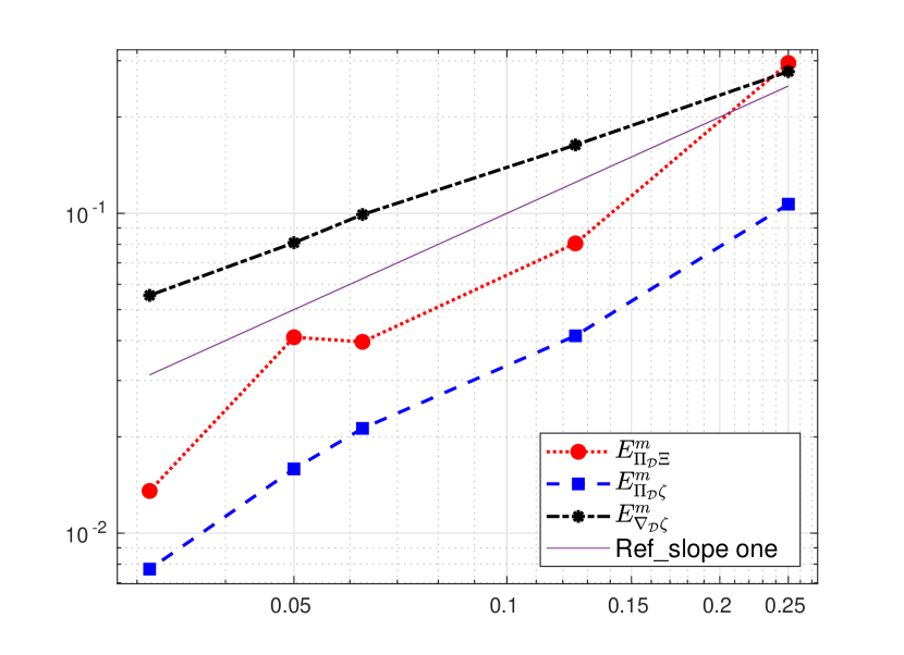
(a) MLP1: triangular meshes.

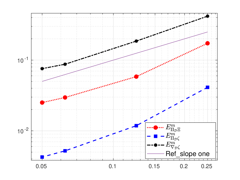
(b) HMM: triangular meshes.

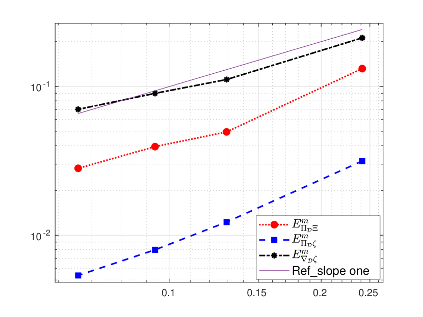
(c) HMM: hexagonal meshes.

Figure 1: Errors verses mesh size.

To assess the accuracy of scheme and validate key theoretical estimates on $\Pi_{\mathcal{D}}\zeta(u)$, $\nabla_{\mathcal{D}}\zeta(u)$ and $\Pi_{\mathcal{D}}\Xi(u)$, we compute the errors, for each of these quantities of interest, between the reference quantity computed on the finest mesh of each family, and the interpolate on the finest mesh of the quantity computed on each mesh of the family. In case of the MLP1 scheme, the interpolation is performed using the values of the coarse $\mathbb{P}^{1}$ piecewise linear function at the vertices of the fine mesh. For HMM, we use the following algorithm to compute the interpolate $I_{R}w$ of a quantity $w\in X_{\mathcal{D},0}$ on the finest mesh:

1. For each $x^{f}$ center of a fine cell or edge, find a coarse mesh $K^{c}$ that contains $x^{f}$.

2. Set the value $(I_{R}w)_{f}$ on this fine cell or edge by a linear interpolation of $w$ in $K^{c}$, that is:

   $$(I_{R}w)_{f}=w_{K^{c}}+\nabla_{K^{c}}w\cdot(x^{f}-x_{K^{c}}).$$

This algorithm is suitable for quantities $w$ which are expected, from the model, to have a gradient – in our case, this means $w=\zeta(u)$. However, when $w$ corresponds to a quantity whose gradient may not be defined (e.g., $w=\Xi(u)$), this interpolation algorithm can lead to very bad values; in that case, we resort to a simpler interpolation by setting $(I_{R}w)_{f}=w_{K^{c}}$.

The following relative errors based on the averages of over 100 random simulations of the Brownian motion are used in the comparison plots, see Figures 1 and 3:

$$E^{m}_{\Pi_{\mathcal{D}}\zeta}={} \frac{\mathbb{E}\left[\left\|\Pi_{\mathcal{D}}\zeta(u_{R})-\Pi_{\mathcal{D}}I_{R}(\zeta(u_{m}))\right\|_{L^{2}(\Theta_{T})}^{2}\right]^{\frac{1}{2}}}{\mathbb{E}\left[\left\|\Pi_{\mathcal{D}}\zeta(u_{R})\right\|_{L^{2}(\Theta_{T})}^{2}\right]^{\frac{1}{2}}},$$

$$E^{m}_{\nabla_{\mathcal{D}}\zeta}={} \frac{\mathbb{E}\left[\left\|\nabla_{\mathcal{D}}\zeta(u_{R})-\nabla_{\mathcal{D}}I_{R}(\zeta(u_{m}))\right\|_{L^{2}(\Theta_{T})}^{2}\right]^{\frac{1}{2}}}{\mathbb{E}\left[\left\|\nabla_{\mathcal{D}}\zeta(u_{R})\right\|_{L^{2}(\Theta_{T})}^{2}\right]^{\frac{1}{2}}},$$

$$E^{m}_{\Xi}={} \frac{\mathbb{E}\left[\int_{\Theta}\left|\Pi_{\mathcal{D}}\Xi(u^{(T)}_{R})-\Pi_{\mathcal{D}}I_{R}(\Xi(u^{(T)}_{m}))\right|\right]}{\mathbb{E}\left[\int_{\Theta}\Pi_{\mathcal{D}}\Xi(u^{(T)}_{R})\right]}$$

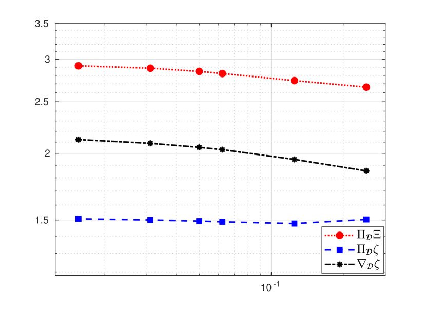
(a) MLP1: triangular meshes.

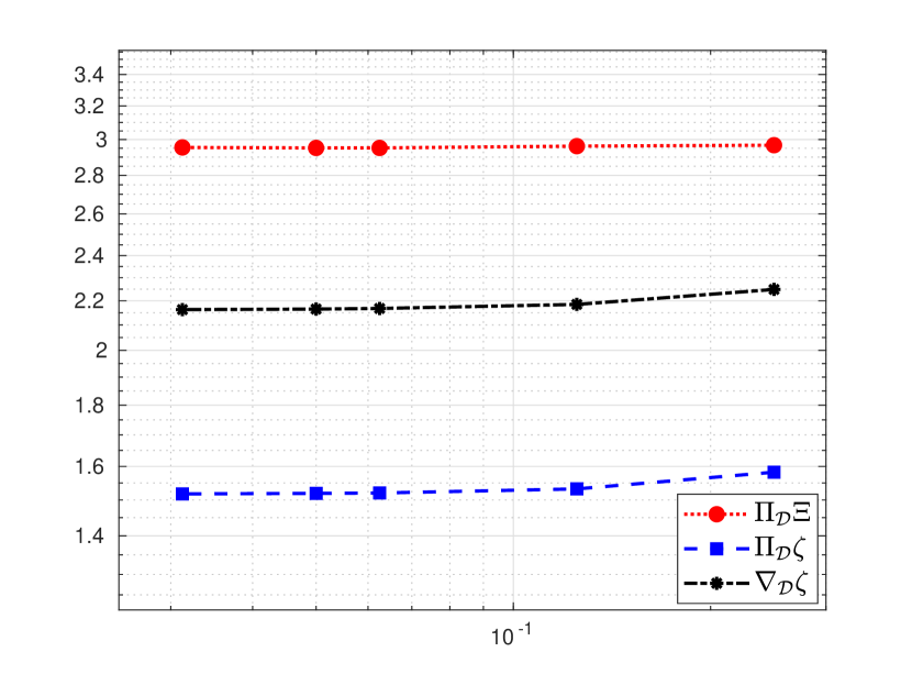
(b) HMM: triangular meshes.

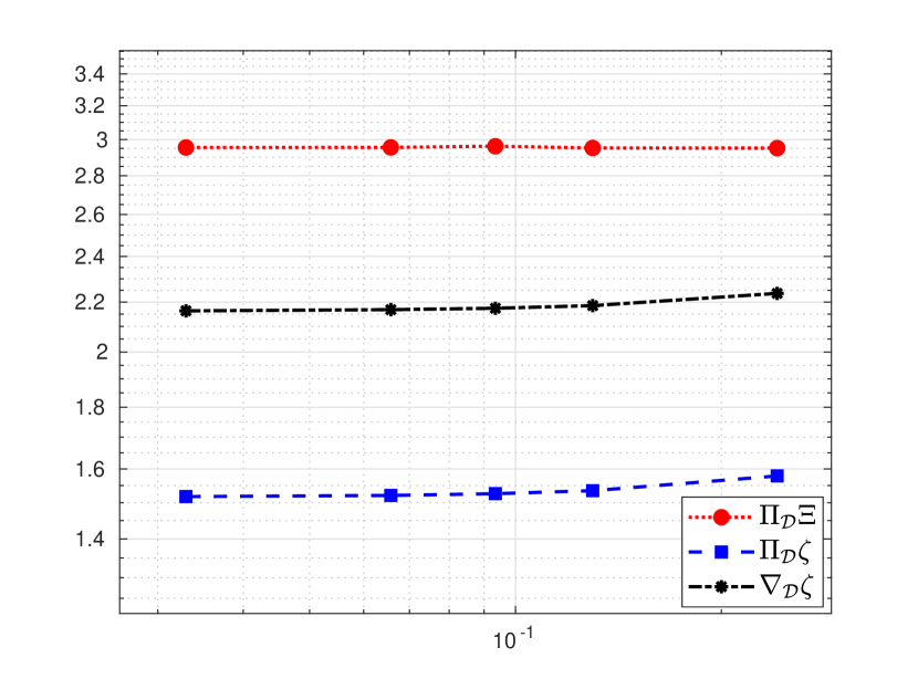
(c) HMM: hexagonal meshes.

Figure 2: Norms of $\Pi_{\mathcal{D}}\zeta(u)$, $\nabla_{\mathcal{D}}\zeta(u)$ and $\Pi_{\mathcal{D}}\Xi(u)$ versus mesh size.

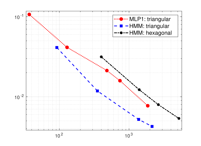
(a) Error $E^{m}_{\Pi_{\mathcal{D}}\zeta}$.

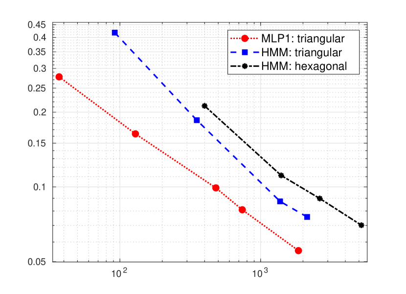
(b) Error $E^{m}_{\nabla_{\mathcal{D}}\zeta}$.

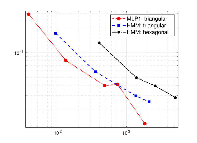
(c) Error $E^{m}_{\Pi_{\mathcal{D}}\Xi}$.

Figure 3: Errors versus Ndofs.

In Figure 1, comparisons of the error estimates with the mesh sizes are provided. All the quantities shows convergence, but we note a larger magnitude of the error for $\Pi_{\mathcal{D}}\Xi$ with the HMM scheme on hexagonal meshes; it can probably be explained by the rougher interpolation process used for this quantity (which does not use any reconstruction in the cells). The average rate of convergence remains around 1 for each quantity. We also tested the validity of the theoretical bounds on $\Pi_{\mathcal{D}}\zeta(u)$, $\nabla_{\mathcal{D}}\zeta(u)$ and $\Pi_{\mathcal{D}}\Xi(u)$ by plotting the respective norms of these quantities in Figure 2. Figure 3 shows comparisons of the gradient schemes in terms of their algebraic complexity. For this, we plot the error estimates for each of the quantity versus their number of degrees of freedom (Ndofs). In computing the Ndofs for the HMM scheme, we only used the number of edges since the cell unknowns can be eliminated using static condensation. These plots show, for a given mesh family, a slight advantage to HMM for the approximation of $\Pi_{\mathcal{D}}\zeta(u)$, and a slight advantage of MLP1 for $\nabla_{\mathcal{D}}\zeta(u)$; the approximations of $\Pi_{\mathcal{D}}\Xi(u)$ are similar (despite a rougher interpolation of this quantity for the HMM scheme).

7 Conclusion

We presented a generic numerical analysis, based on the GDM framework, of the stochastic Stefan problem driven by a multiplicative noise. Using discrete functional analysis tools and the Skorohod theorem, we showed the compactness of the solution to the gradient scheme. We then proved the existence of weak martingale solution and obtained the convergence of the approximate solution. Though these results are available to all of the methods that lies under the hood of the GDM framework, we chose MLP1 and HMM to illustrate them. We observed that, under the influence of multiplicative noise, the overall numerical approximations are reasonably good and corroborate the theoretical results.

8 Acknowledgment

This work was partially supported by the Australian Government through the Australian Research Council’s Discovery Projects funding scheme (grant number DP220100937).

References

- [1] Viorel Barbu and Giuseppe Da Prato “The two phase stochastic Stefan problem” In Probability theory and related fields 124.4 Springer, 2002, pp. 544–560
- [2] Zdzisław Brzeźniak “On stochastic convolution in Banach spaces and applications” In Stochastics: An International Journal of Probability and Stochastic Processes 61.3-4 Taylor & Francis, 1997, pp. 245–295
- [3] Zdzislaw Brzeźniak, Erich Carelli and Andreas Prohl “Finite-element-based discretizations of the incompressible Navier–Stokes equations with multiplicative random forcing” In IMA Journal of Numerical Analysis 33.3 Oxford University Press, 2013, pp. 771–824
- [4] Giuseppe Da Prato and Jerzy Zabczyk “Stochastic Equations in Infinite Dimensions”, Encyclopedia of Mathematics and its Applications Cambridge University Press, 2014 DOI: 10.1017/CBO9781107295513
- [5] Lars Diening, Martina Hofmanová and Jörn Wichmann “An averaged space-time discretization of the stochastic -Laplace system” In Numer. Math. 153.2-3, 2023, pp. 557–609 DOI: 10.1007/s00211-022-01343-7
- [6] Jérôme Droniou, Robert Eymard, Thierry Gallouët, Cindy Guichard and Raphaele Herbin “The gradient discretisation method” Springer, 2018
- [7] Jérôme Droniou, Robert Eymard and Cindy Guichard “Uniform-in-time convergence of numerical schemes for Richards’ and Stefan’s models” In Finite Volumes for Complex Applications VII-Methods and Theoretical Aspects: FVCA 7, Berlin, June 2014, 2014, pp. 247–254 Springer
- [8] Jérôme Droniou, Beniamin Goldys and Kim-Ngan Le “Design and convergence analysis of numerical methods for stochastic evolution equations with Leray–Lions operator” In IMA Journal of Numerical Analysis 42.2, 2021, pp. 1143–1179 DOI: 10.1093/imanum/draa105
- [9] Jérôme Droniou and Kim-Ngan Le “The Gradient Discretization Method for Slow and Fast Diffusion Porous Media Equations” In SIAM Journal on Numerical Analysis 58.3, 2020, pp. 1965–1992 DOI: 10.1137/19M1260165
- [10] Charles M. Elliott “Error Analysis of the Enthalpy Method for the Stefan Problem” In IMA Journal of Numerical Analysis 7, 1987, pp. 61–71
- [11] Robert Eymard, Pierre Féron, Thierry Gallouët, Raphaèle Herbin and Cindy Guichard “Gradient schemes for the Stefan problem” In International Journal On Finite Volumes, 2013, pp. Volume–10
- [12] István Gyöngy “Lattice approximations for stochastic quasi-linear parabolic partial differential equations driven by space-time white noise II” In Potential Analysis 11 Springer, 1999, pp. 1–37
- [13] Erika Hausenblas “Finite Element Approximation of Stochastic Partial Differential Equations driven by Poisson Random Measures of Jump Type” In SIAM Journal on Numerical Analysis 46.1, 2008, pp. 437–471 DOI: 10.1137/050654141
- [14] Adam Jakubowski “The almost sure Skorokhod representation for subsequences in nonmetric spaces” In Theory of Probability and Its Applications 42.1 SIAM, 1998, pp. 167–174
- [15] Joseph W. Jerome and Michael E. Rose “Error Estimates for the Multidimensional Two-Phase Stefan Problem” In Mathematics of Computation 39.160 American Mathematical Society, 1982, pp. 377–414
- [16] Martin Keller-Ressel and Marvin S Müller “A Stefan-type stochastic moving boundary problem” In Stochastics and Partial Differential Equations: Analysis and Computations 4.4 Springer, 2016, pp. 746–790
- [17] Kunwoo Kim, Zhi Zheng and Richard B Sowers “A stochastic Stefan problem” In Journal of Theoretical Probability 25.4 Springer, 2012, pp. 1040–1080
- [18] Alessandra Lunardi “An introduction to parabolic moving boundary problems” In Functional analytic methods for evolution equations Springer, 2004, pp. 371–399
- [19] Gunter H. Meyer “Multidimensional Stefan Problems” In SIAM Journal on Numerical Analysis 10.3 Society for IndustrialApplied Mathematics, 1973, pp. 522–538
- [20] Annie Millet and Pierre-Luc Morien “On implicit and explicit discretization schemes for parabolic SPDEs in any dimension” In Stochastic Processes and their Applications 115.7 Elsevier, 2005, pp. 1073–1106
- [21] Marvin S Müller “A stochastic Stefan-type problem under first-order boundary conditions” In The Annals of Applied Probability 28.4 JSTOR, 2018, pp. 2335–2369
- [22] Johan Stefan “Über die Theorie der Eisbildung, insbesondere über die Eisbildung im Polarmeere” In Annalen der Physik 278.2 WILEY-VCH Verlag Leipzig, 1891, pp. 269–286
- [23] C. Verdi “Stefan Problems and Numerical Analysis” Springer INdAm Series, 2013, pp. 37–45
- [24] John B Walsh “Finite element methods for parabolic stochastic PDE’s” In Potential Analysis 23 Springer, 2005, pp. 1–43
- [25] Yubin Yan “Galerkin Finite Element Methods for Stochastic Parabolic Partial Differential Equations” In SIAM Journal on Numerical Analysis 43.4, 2005, pp. 1363–1384 DOI: 10.1137/040605278
- [26] Zhongqiang Zhang and George Karniadakis “Numerical methods for stochastic partial differential equations with white noise” Springer, 2017