Quasiperiodicity hinders ergodic Floquet eigenstates

Abstract

Quasiperiodic systems in one dimension can host non-ergodic states, e.g. localized in position or momentum. Periodic quenches within localized phases yield Floquet eigenstates of the same nature, i.e. spatially localized or ballistic. However, periodic quenches across these two non-ergodic phases were thought to produce ergodic diffusive-like states even for non-interacting particles. We show that this expectation is not met at the thermodynamic limit where the system always attains a non-ergodic state. We find that ergodicity may be recovered by scaling the Floquet quenching period with system size and determine the corresponding scaling function. Our results suggest that while the fraction of spatially localized or ballistic states depends on the model’s details, all Floquet eigenstates belong to one of these non-ergodic categories. Our findings demonstrate that quasiperiodicity hinders ergodicity and thermalization, even in driven systems where these phenomena are commonly expected.

The study of localization and ergodicity in quantum many-body systems has long been a prominent topic of research in Condensed Matter Physics. Among these studies, the existence of many-body localization (MBL) and transitions between ergodic and MBL phases in interacting systems is a hot topic, that is currently under intense scrutiny (Šuntajs et al., 2020; Kiefer-Emmanouilidis et al., 2020; Abanin et al., 2021; Khemani et al., 2017; Setiawan et al., 2017; Sierant and Zakrzewski, 2022; Sierant et al., 2023). A different research direction, that dates back to the paradigmatic Anderson localization (Anderson, 1958), focuses in the non-interacting limit, where nontrivial localization properties can already occur and a considerably higher degree of understanding can be attained. Currently, the non-interacting limit is not only of fundamental theoretical interest, but also very relevant experimentally, since it can be simulated in optical lattices, where interactions can be tuned (Bloch, 2005). While in the absence of interactions, any finite amount of random disorder localizes the wave function in 1D short-range Hamiltonians (Abrahams et al., 1979; MacKinnon and Kramer, 1981), non-ergodic ballistic, localized and even multifractal phases can occur in 1D quasiperiodic systems(Biddle and Das Sarma, 2010; Bodyfelt et al., 2014; Liu et al., 2015; Danieli et al., 2015; Ganeshan et al., 2015; Liu et al., 2022; Gonçalves et al., 2022a; Devakul and Huse, 2017; Gonçalves et al., 2023; Wang et al., 2016; Aubry and André, 1980; Ahmed et al., 2022; Lee et al., 2023), in various long-range models Kravtsov et al. (2015); Facoetti et al. (2016); Nosov et al. (2019); Nosov and Khaymovich (2019); Motamarri et al. (2022); Tang and Khaymovich (2022), as well as claimed in some hierarical graphs V.E.Kravtsov et al. (2018); Altshuler et al. (2016); Kravtsov et al. (2018); Tikhonov and Mirlin (2016); Sonner et al. (2017); Tikhonov and Mirlin (2021). A simple but non-trivial paradigmatic model where such physics can be well understood, is the Aubry-André model, for which an energy-independent ballistic-to-localized transition occurs at a finite strength of the quasiperiodic potential (Aubry and André, 1980; Roati et al., 2008).

While the study of localization and ergodicity in periodically driven systems dates back to the periodically kicked quantum rotator (Fishman et al., 1982; Moore et al., 1994; Grempel et al., 1984), it has experienced a resurgence of interest (Ponte et al., 2015a, b; Lazarides et al., 2015; Abanin et al., 2016; Rehn et al., 2016; Gopalakrishnan et al., 2016; Ray et al., 2018a; D’Alessio and Rigol, 2014; Russomanno et al., 2015; Regnault and Nandkishore, 2016; Kim et al., 2014; Canovi et al., 2016; Khemani et al., 2016) due to the possibility to emulate time-periodic Hamiltonians and quasiperiodic potentials in experiments involving ultracold atoms and trapped ions experiments (Eckardt, 2017; Bordia et al., 2017; Shimasaki et al., 2022). These (non-equilibrium) Floquet systems are very appealing, because on the one hand, they provide a means to realize complex effective time-independent Hamiltonians by careful choice of the driving protocol (Struck et al., 2012; Goldman and Dalibard, 2014; Struck et al., 2013; Jamotte et al., 2022; Aidelsburger et al., 2013; Miyake et al., 2013; Jotzu et al., 2014; Wu et al., 2016; Aidelsburger et al., 2015), and, on the other hand, they can support novel phases of matter with no equilibrium counterpart (Potter et al., 2016; Yates et al., 2022; Kitamura and Aoki, 2022; Jiang et al., 2011; Kitagawa et al., 2010; Rudner et al., 2013). A notable example of the latter arises in interacting 1D quasiperiodic systems, where driving can induce a transition from non-ergodic many-body-localized states to ergodic states (D’Alessio and Rigol, 2014; Lazarides et al., 2015; Abanin et al., 2016; Bordia et al., 2017; Ray et al., 2018a).

For 1D quasiperiodic systems, the localization phase diagram of the Floquet Hamiltonian can show a complex structure at high frequencies, even in the non-interacting limit. Non-ergodic ballistic, localized and multifractal phases and energy-dependent transitions between them can arise in the Floquet Hamiltonian (Prosen et al., 2001; Qin et al., 2014; Dai et al., 2018; Čadež et al., 2019; Roy et al., 2018; Zhang et al., 2022; Sarkar et al., 2021), even if they are not present in the undriven model. Interestingly, one of the widely studied non-interacting models was recently realized experimentally in cold atoms (Shimasaki et al., 2022). For lower frequencies, transitions into a non-ergodic delocalized phase were reported theoretically even in the absence of interactions (Ray et al., 2018b; Romito et al., 2018), where a connection with the frequency-induced ergodic-to-MBL transition observed experimentally in Ref. (Bordia et al., 2017) was made. However, these theoretical studies were mostly carried out for fixed system sizes, possibly motivated by the limited sizes in cold atom experiments. It is however of paramount importance to understand the nature of the thermodynamic-limit state, which requires a detailed finite-size scaling analysis.

In this paper we carry out a finite-size scaling analysis at large driving periods for a periodically-driven Aubry-André model and show that, contrary to previous expectations (Ray et al., 2018b; Romito et al., 2018), quenches between ballistic and localized states yield non-ergodic Floquet states in the thermodynamic limit for any finite driving period. We find that quenches between localized states yield localized Floquet states as expected (Hatami et al., 2016; Agarwal et al., 2017; Wauters et al., 2019; Ray et al., 2018b), and quenches between (non-ergodic) ballistic states yield ballistic states. However, for quenches between ballistic and localized states, while ergodic states can be observed for fixed system sizes in the limit of a large driving period, they flow either to non-ergodic ballistic or localized states as the system size increases, with fractions that depend on the center of mass of the quench.

I Model and methods

We consider a periodically-driven Aubry-André model (Aubry and André, 1980; Ray et al., 2018b), a tight-binding chain of spinless fermions with nearest-neighbor hoppings and with time-periodic quenches in the quasiperiodic potential. The Hamiltonian reads

$$H(t) = -J\sum_{n=0}^{L-1}c_{n}^{\dagger}c_{n+1}+\textrm{h.c.}$$ (1)

$$+\sum_{n}V[1+\epsilon f(t)]\cos(2\pi\tau n+\phi)c_{n}^{\dagger}c_{n}$$

where $c_{n}^{\dagger}$ creates a particle at site $n$, and $L$ is the number of sites/system size. $J$ is the nearest-neighbor hoppings amplitude. We consider twisted boundary conditions, i.e. $c_{L}=c_{0}e^{i\kappa}$, with phase twist $\kappa$. The last term contains a time-dependent quasiperiodic modulation of strength $V[1+\epsilon f(t)]$, where $f(t)\equiv\Theta(t-T/2)-\Theta(T/2-t)$ implements quenches of period $T$ between Hamiltonians $H_{\pm}$ with quasiperiodic potentials of strength $V[1\pm\epsilon]$.

Henceforth, we refer to $V$ as the center of mass of the quench and set $J=1$. For $\epsilon=0$, the Hamiltonian loses its time-dependence and we recover the static Aubry-André model, for which there is a ballistic (localized) phase for $|V|<|J|$ ($|V|>|J|$) (Aubry and André, 1980).

Throughout the paper, we take $\tau=2/(\sqrt{5}-1)$ (inverse of the golden ratio) in the numerical calculations. To avoid boundary defects, we consider rational approximations of $\tau$, $\tau_{c}^{(n)}=F_{n-1}/F_{n}$, for each system size $L_{n}=F_{n}$, where $F_{n}$ is the $n$-th Fibonacci number (Azbel, 1979; Kohmoto, 1983). This choice ensures that the system has a single unit cell for any system size, being therefore incommensurate. We will consider system sizes corresponding to Fibonacci numbers in the range $L\in[377-6765]$ ($[F_{14}-F_{20}]$). Finally, we also average all the results over random configurations of the phase twist $\kappa$ and the phase $\phi$ of the quasiperiodic potential.

The time-evolution operator $U(T)$ for the periodic quench can be written as

$$U(T)=e^{-i\int_{0}^{T}H(t)\textrm{ }dt}=e^{-iH_{-}T/2}e^{-iH_{+}T/2}\equiv e^{-iH_{F}T},$$ (2)

where in the last equality we defined the Floquet Hamiltonian $H_{F}$. The eigenvalues and eigenstates of this Hamiltonian correspond respectively to the Floquet quasienergies $E_{\alpha}$ and eigenstates $\left|\bm{\psi}^{\alpha}\right\rangle=\sum_{n}\psi_{n}^{\alpha}\left|n\right\rangle$, that we will study throughout this paper.

To study the ergodicity of the eigenstates we analysed the energy level statistics of quasienergies (Haake, 2001; Altland and Zirnbauer, 1997), while to study their localization properties, we computed inverse participation ratios for the Floquet eigenstates (Janssen, 2004; Evers and Mirlin, 2008).

For the level statistics analysis, we first order the quasienergies $\{E_{\alpha}\}$ in the interval $]-\pi,\pi]$ and then compute consecutive spacings between them, $s_{\alpha}=E_{\alpha+1}-E_{\alpha}$. We will study the distribution of ratios $r_{\alpha}$ defined as (Oganesyan and Huse, 2007; Atas et al., 2013),

$$r_{\alpha}=\frac{{\rm min}(s_{\alpha},s_{\alpha-1})}{{\rm max}(s_{\alpha},s_{\alpha-1})}.$$ (3)

Non-ergodic energy levels are expected to show Poisson (or even sub-Poisson) statistics, following a distribution $P(r)=2/(1+r)^{2}$, with $\langle r\rangle\approx 0.386$, while ergodic energy levels show level repulsion, following the Gaussian unitary ensemble (GUE) distribution with $\langle r\rangle\approx 0.6$ for systems belonging to the unitary class (which is the case for our model in Eq. (1), that breaks time-reversal symmetry due to the phase twists). We note that in fact, since $E_{\alpha}$ are phases, they should follow circular ensembles in the ergodic cases (D’Alessio and Rigol, 2014). Nonetheless, the distributions obtained for the circular ensembles should coincide with the distributions of the corresponding Gaussian ensembles in the thermodynamic limit (D’Alessio and Rigol, 2014).

For the localization analysis, we computed the real- and momentum-space inverse participation ratios, given respectively for the Floquet eigenstate $\left|\psi^{\alpha}\right\rangle$ by:

$$\begin{aligned} {\rm IPR}^{\alpha}=\Bigl{(}\sum_{n}|\psi_{n}^{\alpha}|^{2}\Bigr{)}^{-2}\sum_{n}|\psi_{n}^{\alpha}|^{4}\propto L^{-D_{r}}\\ {\rm IPR}_{K}^{\alpha}=\Bigl{(}\sum_{k}|\Phi_{k}^{\alpha}|^{2}\Bigr{)}^{-2}\sum_{k}|\Phi_{k}^{\alpha}|^{4}\propto L^{-D_{k}}\end{aligned},$$ (4)

where $\Phi_{k}^{\alpha}=L^{-d/2}\sum_{n}e^{-2\pi\textrm{i}nk}\psi_{n}^{\alpha}$ is the momentum-space wavefunction, and $d=1$ the system’s dimension. Since our model does not have any other special basis, other than the real- and momentum-space ones, we focus only on the above two IPRs. States with different localization properties can therefore be distinguished by these quantities: (i) ballistic: $D_{r}=d$ and $D_{k}=0$; (ii) localized: $D_{r}=0$ and $D_{k}=d$; fractal/multifractal: $0<D_{r},D_{K}<d$; (iii) diffusive: $D_{r}=D_{k}=d$. Henceforth, we define the inverse participation ratios averaged (geometrically) over all eigenstates and configurations of $\phi$ and $\kappa$ as $\mathcal{I}_{r}=\langle{\rm IPR}^{\alpha}\rangle_{\phi,\kappa,\alpha}$ and $\mathcal{I}_{k}=\langle{\rm IPR}_{K}^{\alpha}\rangle_{\phi,\kappa,\alpha}$. We averaged over a number of configurations in the interval $N_{c}\in[400,10^{4}]$, choosing the larger numbers of configurations for the smaller system sizes.

II Results

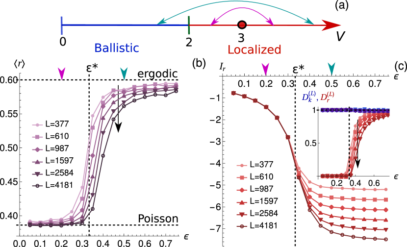
Figure 1: (a) Floquet-drive location on the static phase diagram of the Aubry-André model. The arrows indicate two amplitudes $\epsilon$ of quasiperiodic potentials used in the periodic quench for $V=3$, also shown in (b,c): quench between localized states (magenta) and between ballistic and localized states (cyan). (b) $\langle r\rangle$ for $V=3$ and $T=500$, as a function of $\epsilon$, for different system sizes $L$. The vertical dashed line indicates the value $\epsilon=\epsilon^{*}$ above which ballistic and localized states start being quenched, while the horizontal dashed lines indicate $r_{{\rm GUE}}$ (ergodic) and $r_{{\rm Poisson}}$. The arrow points towards larger $L$. (c) $\mathcal{I}_{r}$ for the same parameters as in (b). The inset contains the real- and momentum-space finite-size fractal dimensions defined in Eq. (5).

Quench’s center of mass at localized phase.— We start by studying the case where the center-of-mass of the quench lies in the localized phase. For this purpose, we set $V=3$, a large driving period $T=500$ and vary the Floquet amplitude $\epsilon$. In Fig. 1, we show the results for $\langle r\rangle$ and $I_{r}$, averaged over all the Floquet eigenstates. In the inset of Fig. 1(c), we also show the finite-size fractal dimensions $D_{r}^{(L)}\equiv\mathcal{D}^{(L)}(\mathcal{I}_{r})$ and $D_{k}^{(L)}\equiv\mathcal{D}^{(L)}(\mathcal{I}_{k})$, where

$$\mathcal{D}^{(L=L_{n})}(\mathcal{I})=\frac{\log[\mathcal{I}(L_{n+1})]-\log[\mathcal{I}(L_{n})]}{\log(L_{n+1})-\log(L_{n})},$$ (5)

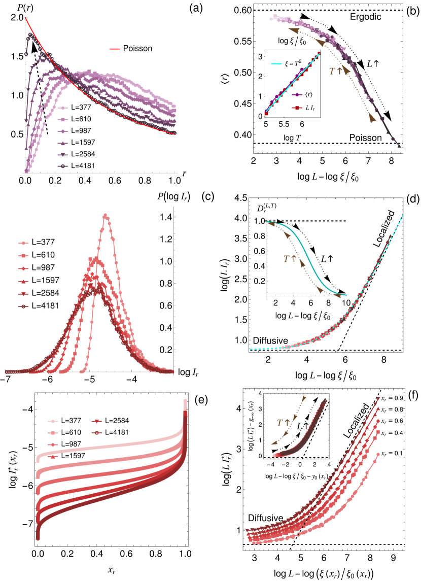
Figure 2: Quench’s center of mass in localized phase: results for $V=3,\epsilon=0.45>\epsilon^{*}$. (a) $P(r)$ distribution at $T=150$ for different system sizes. The arrow points towards increasing $L$ and the full red line indicates the Poisson distribution $P(r)=2/(1+r)^{2}$. The distributions were computed by binning, where each data point corresponds to the bin center. (b) Scaling collapse of $\langle r\rangle$ calculated for different driving periods $T$ belonging to the interval $T\in[125,650]$ and $L\in[377,4181]$ (see Appendix for details on the scaling collapse). The correlation lengths $\xi$ were extracted from the scaling collapse and $\xi_{0}=\xi(T=125)$. The black (brown) arrows point towards increasing $L$ ($T$). The inset shows $\log(\xi/\xi_{0})$ as function of $\log T$, obtained from both the collapses of $\langle r\rangle$ and of $L\mathcal{I}_{r}$ done in (d). The cyan line was obtained by fitting for the data points at $6$ largest $T$-values (combining the data from $\langle r\rangle$ and $L\mathcal{I}_{r}$ ), yielding a power-law $\xi\sim T^{2}$. (c) Distribution $P(\log\mathcal{I}_{r})$ for $T=150$ and different system sizes. (d) Scaling collapse of $L\mathcal{I}_{r}$, again for $T\in[125,650]$. The large $L$ localized behaviour $L\mathcal{I}_{r}\sim L$ and large $\xi$ (or $T$) diffusive behaviour $L\mathcal{I}_{r}\sim L^{0}$ are indicated by the black dashed lines. We find that $\log(L\mathcal{I}_{r})$ is well fitted by the expression $g(y)=g_{-\infty}+\log(1+e^{y-y_{0}})$, where $y=\log L-\log\xi/\xi_{0}$, shown in the dashed cyan line. We obtain the fractal dimension from this fit through $D_{r}^{(L,T)}=1-[\log(L\mathcal{I}_{r})]^{\prime}$, and show in the inset, in full cyan. (e) $\log\mathcal{I}_{r}^{*}(x_{r})$ defined in Eq. (8) and below it, for different $L$ and for $T=300$. (f) Scaling collapse of $\log\mathcal{I}_{r}^{*}(x_{r})$ for different values of $x_{r}$ indicated in the figure. We note that the computed $\xi(x_{r})$ are identical for the different $x_{r}$, as shown in Appendix B. By fitting the collapsed data for different $x_{r}$ to $g^{(x_{r})}(y)=g_{-\infty}(x_{r})+\log(1+e^{y-y_{0}(x_{r})})$ we were able to collapse all the curves into an universal curve shown in the inset. The fitted parameters $g_{-\infty}(x_{r})$ and $y_{0}(x_{r})$ are shown in Fig. 9(a) of the Appendix.

such that $D_{p}^{(\infty)}=D_{p},\textrm{ }p=r,k$. When $\epsilon<\epsilon^{*}=1-2/V(V>2)$, the quench is only between localized states, as illustrated in Fig. 1(a). In this case, we see that up to weak finite-size effects, $\langle r\rangle=r_{\textrm{Poisson}}$, $D_{r}=0$ and $D_{k}=1$, clearly showing that the Floquet eigenstates are non-ergodic and localized. Once $\epsilon\geq\epsilon^{*}$, we start quenching between ballistic and localized phases, which is accompanied by a sharp increase in $\langle r\rangle$, that approaches $r_{\textrm{GUE}}$ as $\epsilon$ is increased; and in $D_{r}^{(L)}$, that approaches $1$, while we still have $D_{k}^{(L)}\approx 1$. Upon initial observation, this behaviour could indicate a transition into a diffusive ergodic phase. However, when $L$ is increased, there is a clear overall decrease both in $\langle r\rangle$ and in $D$, which is already a clear indication of the fragile nature of the ergodic-phase candidate.

The instability of the ergodic phase is further corroborated in Fig. 2, where we also set $V=3$ and choose $\epsilon=0.45>\epsilon^{*}$, to quench between ballistic and localized states. In Fig. 2(a) we show the distribution of ratios $P(r)$ for fixed $T=150$ and for different system sizes. There, we can clearly see that the distribution of ratios transitions from exhibiting level repulsion to closely resembling the Poisson distribution as $L$ is increased. Concurrently, Fig. 2(c) demonstrates that the distribution of $\log\mathcal{I}_{r}$ for the same $T$ is almost entirely converged for the larger $L$ used, implying the localization of all (or nearly all) states [note that $D_{k}\approx 1$, as shown in Fig. 1(c)].

The results so far are in support of an ergodic phase only surviving when $T\rightarrow\infty$ at finite $L$. With this in mind, we define a correlation length $\xi(T)$ that diverges when $T\rightarrow\infty$, such that when $L\ll\xi$, the system is ergodic while when $L\gg\xi$, the system is non-ergodic. Close to the transition to the diffusive ergodic phase, that is, for large enough $T$, we assume that $\xi$ diverges as a power-law in $T$, $\xi\sim T^{\beta}$, with an unknown exponent $\beta$ that may depend on the model parameters. We also assume that in this regime, $\langle r\rangle$ follows a one-parameter scaling function that satisfies,

$$\langle r\rangle=f(L/\xi)=\begin{cases}r_{\textrm{GUE}}&,L\ll\xi\\ \approx r_{\textrm{Poisson}}&,L\gg\xi\end{cases}.$$ (6)

In a similar way, we also assume $\mathcal{I}_{r}$ follows the one-parameter scaling ansatz $\mathcal{I}_{r}=L^{\mu}g(L/\xi)$ at large enough $T$. Using that for $\xi/L\rightarrow\infty$, $\mathcal{I}_{r}=L^{\mu}g(0)\sim L^{-1}$ (diffusive and ergodic), we get that $\mu=-1$. In the limit $L/\xi\rightarrow\infty$, the states are localized, $\mathcal{I}_{r}\sim L^{0}$. We therefore have the following limits for $g(L/\xi)$

$$L\mathcal{I}_{r}=g(L/\xi)\sim\begin{cases}1&,L\ll\xi\\ L/\xi&,L\gg\xi\end{cases}.$$ (7)

As a consequence $\mathcal{I}_{r}\simeq 1/\min(L,\xi)$, meaning that $\xi(T)$ is, indeed, a $T$-dependent localization length of the model. Indeed, as soon as $L\ll\xi$, the states do not know about $\xi$ and look like ergodic ones, while in the opposite limit of $L\gg\xi$, the boundary conditions are not important and all the states are localized at a distance $\sim\xi$.

We note that here we are not considering the scaling function for $\mathcal{I}_{k}$, since $\mathcal{I}_{k}\sim L^{-1}$ both in the diffusive and localized phases.

In Figs. 2(b,d), we collapse data for different periods in the range $T\in[125,650]$ and for different $L$, showing the validity of the scaling ansatzes in Eqs. (6), (7). In Appendix B we provide precise details on how the scaling collapses were computed. From the collapses, we can extract $\xi(T)$ that we plot in the inset of Fig. 2(b). In this figure, we see that $\xi(T)$ acquires a power-law behaviour at large $T$, as expected, giving compatible results when extracted from the scaling collapses of $\langle r\rangle$ and $\mathcal{I}_{r}$. By fitting the power-law at large $T$, we extract $\beta=2$. We note however, that this exponent is non-universal and depends on the model’s parameters as we demonstrante below for other examples.

The good scaling collapses in Figs. 2(b,d) confirm our previous affirmations: (i) when the system size increases for fixed $T$ (that is, fixed $\xi$), the Floquet eigenstates flow to a non-ergodic localized phase; (ii) if $T$ is increased for fixed $L$, the system flows to a diffusive ergodic phase. This implies that the limits $T\rightarrow\infty$ and $L\rightarrow\infty$ do not commute.

Next, in order to inspect how different parts of the $\mathcal{I}_{r}$ distribution evolve with $T$ and $L$, similarly to Roy et al. (2018), we define the fraction of states $x_{r}$ for which the average IPR is bounded by $\mathcal{I}_{r}=\mathcal{I}_{r}^{*}$, given by

$$x_{r}=\int_{-\infty}^{\log\mathcal{I}_{r}^{*}}P(y^{\prime})dy^{\prime}$$ (8)

where $y^{\prime}=\log\mathcal{I}_{r}$. In Fig. 2(e) we plot $\log\mathcal{I}_{r}^{*}(x_{r})$, showing that it is a smooth function of $x_{r}$. To analyse how $\mathcal{I}_{r}^{*}$ evolves for different fractions $x_{r}$, in Fig. 2(f) we perform the $x_{r}$-dependent collapse of $\log L\mathcal{I}_{r}^{*}(x_{r})$. We observe that the corresponding scaling functions have the properties of Eq. (7) for the studied fractions of states $x_{r}$ and can even be collapsed into a single universal curve given in the inset of Fig. 2(f), as detailed in the Figure’s caption. Noteworthy, we checked that the correlation lengths $\xi(x_{r})$ obtained from the scaling collapses at different $x_{r}$ are almost independent of $x_{r}$ at large $T$, as we show in Appendix B.

In Appendix A, we also studied the case when the quench’s center of mass lies in the ballistic phase. In this case, we observed that the Floquet eigenstates also become non-ergodic in the thermodynamic limit, but ballistic, instead of localized.

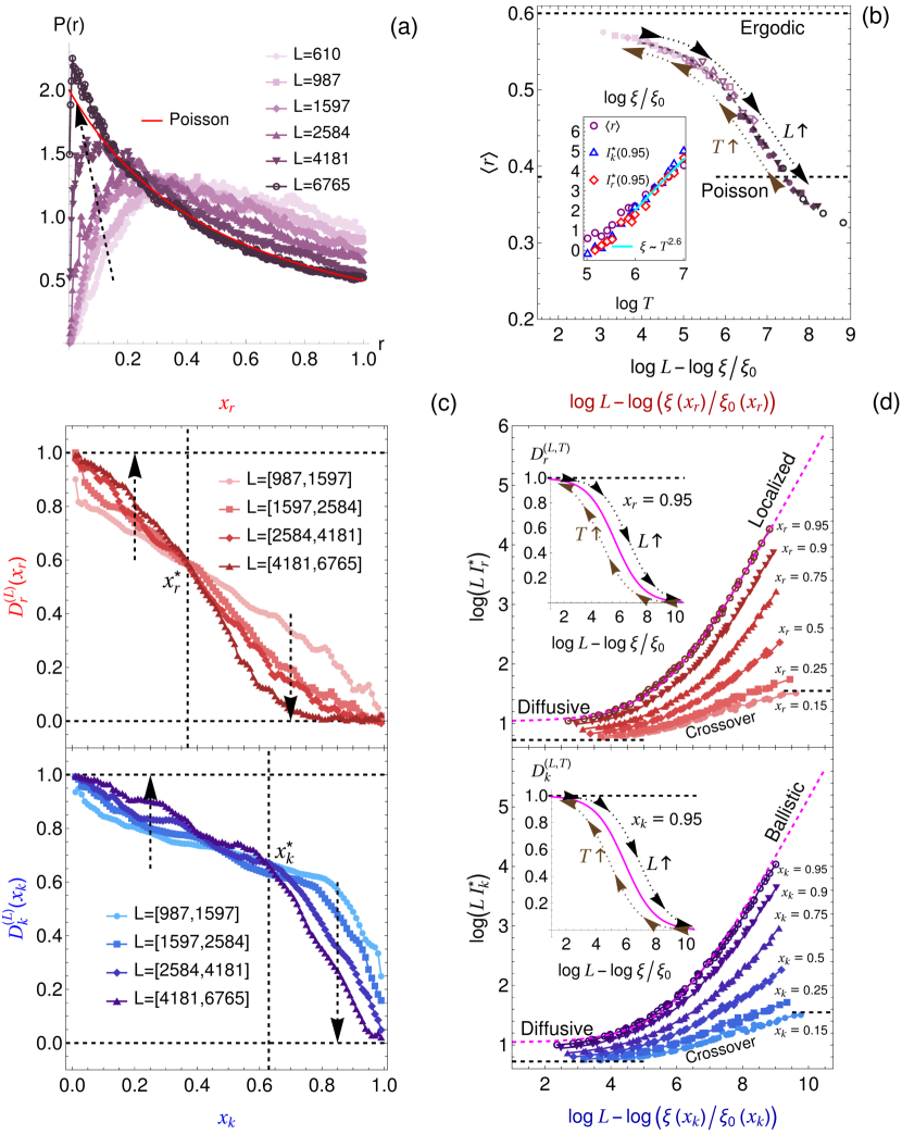
Figure 3: Quench’s center of mass at critical point: results for $V=2,\epsilon=0.2$. (a) $P(r)$ distribution for $T=250$, for different system sizes $L$. (b) Scaling collapses of $\langle r\rangle$ calculated for driving periods $T$ belonging to the interval $T\in[125,1100]$ and for $L\in[1597-6765]$ (see Appendix for details on the scaling collapse). The inset shows $\log(\xi/\xi_{0})$ as function of $\log T$, obtained from the data collapses of $\langle r\rangle$, $L\mathcal{I}_{r}^{*}(x_{r}=0.95)$ and $L\mathcal{I}_{k}^{*}(x_{k}=0.95)$ shown in (d). The cyan line was obtained by fitting for the data points at $7$ largest $T$-values (combining the data from the three shown collapses), yielding a power-law $\xi\sim T^{2.6}$. (c) Fractal dimensions $D_{r}^{(L)}(x_{r})\equiv\mathcal{D}\big{(}\mathcal{I}_{r}^{*}(x_{r})\big{)}$ (top) and $D_{k}^{(L)}(x_{k})\equiv\mathcal{D}\big{(}\mathcal{I}_{k}^{*}(x_{k})\big{)}$ (bottom) [see Eq. (5)], for $T=125$. (d) Scaling collapses for $\log\big{(}L\mathcal{I}_{r}^{*}(x_{r})\big{)}$ (top) and $\log\big{(}L\mathcal{I}_{k}^{*}(x_{k})\big{)}$ (bottom), for different $x_{r}$ and the same range of $T$ and $L$ as in (a). The magenta dashed lines correspond to fits of the collapsed data for $x_{r}=0.95$ (top) and $x_{k}=0.95$ (bottom) to the function $g(y)=g_{-\infty}+\log(1+e^{y-y_{0}})$, with $y=\log L-\log\xi/\xi_{0}$. In the inset, we show the $L$- and $T$-dependent fractal dimensions obtained from these fits through $D_{r(k)}^{(L,T)}\equiv 1-[\log(L\mathcal{I}_{r(k)})]^{\prime}$.

Quench’s center of mass at critical point.— We now turn to the case where the quench’s center of mass is exactly at the critical point, that is, $V=2$. This is studied in Fig. 3. Similarly to the previous case, Fig. 3(a) reveals the evolution breakdown of level repulsion when $L$ increases, for fixed $T$. In Fig. 3(b) we see that a scaling collapse for $\langle r\rangle$ is still possible. It is worth noticing that in this case, however, $\langle r\rangle$ can take values significantly below $r_{\textrm{Poisson}}$ for large $L$. This can however be a finite-size effect arising from the formation of energy gaps that can only be resolved for large enough $L$. In this case, the $P(r)$ distribution should converge to the Poisson distribution in the thermodynamic limit.

The main difference for this quench comparing to the $V=3$ case is that there is clearly a fraction of states that flow to localized behaviour, while the remaining fraction flows to ballistic behaviour, as $L$ is increased. This is illustrated in Fig. 3(c). There, we define $x_{r}$ as in Eq. (8) for $\mathcal{I}_{r}$ and we also define $x_{k}$ using the analogous definition for $\mathcal{I}_{k}$:

$$x_{k}=\int_{-\infty}^{\log\mathcal{I}_{k}^{*}}P(y^{\prime})dy^{\prime}$$ (9)

where $y^{\prime}=\log\mathcal{I}_{k}$. For the following discussion, we define the $x_{p}$-dependent fractal dimensions as $D_{p}^{(L)}(x_{p})=\mathcal{D}\big{(}\mathcal{I}_{p}^{*}(x_{p})\big{)}$ (see Eq. (5)), with $p=r,k$. In Fig. 3(c), we can see that for $x_{r}>x_{r}^{*}\approx 0.35$ (see $x_{r}^{*}$ indicated in the figure), $D_{r}^{(L)}(x_{r})$ decreases with $L$, seemingly towards $0$. Concomitantly, $D_{k}^{(L)}(x_{k})$ increases towards $1$ for $x_{k}<x_{k}^{*}=1-x_{r}^{*}\approx 0.65$. This is an indication that approximately $65\%$ of states are localized in the thermodynamic limit. On the other hand, for the remaining fraction of $\approx 35\%$ states, the results are concomitant with $D_{r}^{(L)}(x_{r}<x_{r}^{*})\rightarrow 1$ and $D_{k}^{(L)}(x_{k}>x_{k}^{*})\rightarrow 0$, as expected for ballistic states.

We note that it might happen that a finite fraction of multifractal states survives in the thermodynamic limit. However, for the available system sizes, all the states seem to flow to localized and ballistic ones. That being the case, only a fraction of multifractal states of measure zero, arising at mobility edges between ballistic and localized states, should survive the thermodynamic limit.

Finally, in Fig. 3(d) we make scaling collapses of $\log L\mathcal{I}_{k}^{*}$ and $\log L\mathcal{I}_{r}^{*}$ for different $x_{r}$ and $x_{k}$. We can see that for large enough $x_{r}$, $D_{r}$ clearly flows from $D_{r}=1$ (diffusive) to $D_{r}=0$ (localized) as $L\rightarrow\infty$ for fixed $T$. In the same way, for large enough $x_{k}$, $\Gamma_{k}$ flows from $D_{k}=1$ (diffusive) to $D_{k}=0$ (ballistic) as $L\rightarrow\infty$ for fixed $T$. For small $x_{r}$ ($x_{k}$), $D_{r}=1$ ($D_{k}=1$) in both the limits $L/\xi\rightarrow\infty$ and $\xi/L\rightarrow\infty$, as indicated by the constant $\log L\mathcal{I}_{r}^{*}$ ($\log L\mathcal{I}_{k}^{*}$) in both these limits. It is nonetheless interesting to notice that even in this case there is a crossover regime at finite $L$ and $T$ indicated in Fig. 3(d).

Dualities and universality at small $T$.— Up to now, we verified that when $L\rightarrow\infty$, the Floquet eigenstates become non-ergodic, as in the static limit. At large $T$, however, there is a very complex structure of mobility edges, and a (quasi)energy-resolved analysis becomes very challenging. On the other hand, for small $T$, such analysis is still possible and elucidating. In Fig. 4(a), we show an example where it can be clearly seen that for small $T$, even though the phase diagram can already be quite complex, clear transitions between ballistic (low IPR) and localized (large IPR) phases can still be found. In the static case, hidden dualities with universal behaviour were found to be behind these transitions (Gonçalves et al., 2022b). Moreover, it was found that ballistic, localized and even critical phases can be understood in terms of renormalization-group flows to simple renormalized effective models (Gonçalves et al., 2022a).

Remarkably, we find that these results can be generalized for the Floquet Hamiltonian. This can be seen by inspecting the dependence of the quasienergies on the potential shift $\varphi\equiv L\phi$ and on the phase twist $\kappa$ (Gonçalves et al., 2022b, a). We illustrate this for two representative ballistic-to-localized transitions in Figs. 4(b,c), where we see that: (i) at the ballistic (localized) phase, the quasienergy dependence on $\kappa$ ($\varphi$) is dominant and the dependence on $\varphi$ ($\kappa$) becomes irrelevant as $L\rightarrow\infty$ (not shown); (ii) the quasienergies become invariant under switching $\kappa$ and $\varphi$ at the critical point. This is exactly the universal behaviour also found for the single-particle energies in the static case (Gonçalves et al., 2022b, a).

With these results in mind, we conjecture that the hidden dualities and RG universality found at small $T$ extend to large $T$, but only for a large enough system size when the system flows to one of the non-ergodic phases. It is however very challenging to verify this conjecture due to the intricate structure of mobility edges at large $T$ and the limited available system sizes.

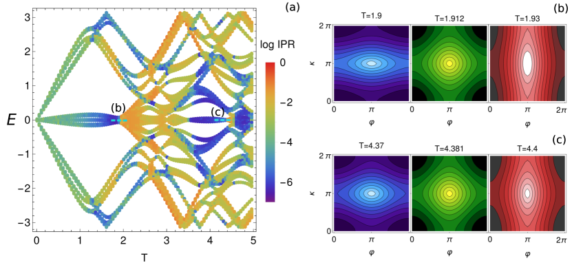
Figure 4: (a) $\log{\rm IPR}$ as a function of quasienergy $E$ and driving period $T$, for $L=987,V=2,\epsilon=0.8$, and for a fixed random choice of $\phi$ and $\kappa$. (b,c) Quasienergy contours (lighter colors correspond to larger quasienergy) in the plane of phases $\varphi\equiv L\phi$ and $\kappa$, for $L=34$ and values of $T$ indicated above each figure, for the $\lfloor L/2\rfloor$-th largest quasienergy (ordered in the interval $]-\pi,\pi]$), that has $E\approx 0$. The results were obtained around the ballistic-to-localized transitions indicated by the dashed cyan lines in (a), with the blue and red figures chosen respectively inside the ballistic and localized phases, and the green figure approximately at the critical point.

III Discussion

Contrary to prior expectations, we have established that time-periodic quenches between non-ergodic ballistic and localized states in non-interacting 1D quasiperiodic systems lead to the emergence of non-ergodic states at the thermodynamic limit, for any finite driving period. To restore ergodicity, the driving period must be scaled with the system size, according to the corresponding scaling functions, which we also determined.

We expect our findings to hold in generic driven non-interacting 1D quasiperiodic systems. Even though delocalized phases were previously reported for small enough driving frequencies, no clear phase with ergodic properties surviving the thermodynamic limit was identified so far.

For instance, in Ref. (Sarkar et al., 2021), a localization-delocalization transition with decreasing driving frequency was recently reported. However, as we detail in Appendix C, the low-frequency extended phases are non-ergodic, either ballistic or multifractal.

Our findings raise interesting further questions, such as quenching outcomes between distinct phases in higher dimensions, where ergodic states can exist in static, non-interacting situations. These results also suggest that finite interactions may be crucial for the observation of driving-induced ergodic to MBL transitions reported experimentally (Bordia et al., 2017). Nonetheless, it is likely that the ergodic to non-ergodic crossover, which we predict for the non-interacting limit, is experimentally accessible. If so, this would allow the experimental determination of the scaling function between the period and the system size which effectively characterises the fragility of the non-interacting ergodic states.

Appendix A Quench’s Center of mass deep in ballistic phase

In this Appendix section, we study a periodic quench with a center-of-mass in the ballistic phase. In Fig. 5, we see that a quench that only mixes ballistic states, gives rise to ballistic states, as signaled by $\langle r\rangle=r_{\textrm{Poisson}},D=1$ and $D_{k}=0$ for $\epsilon<\epsilon^{*}=2/V-1(V<2)$. For $\epsilon\geq\epsilon^{*}$, we see that even though there is a sudden increase in $\langle r\rangle$ and $D_{k}$ for fixed system sizes towards what is expected in an ergodic phase (similarly to the increase in $\langle r\rangle$ and $D$ when the quench was centered at the localized phase, in Fig. 1), the latter behaviour is not robust when $L$ is increased. To prove this point in a more precise way, we fix $\epsilon=0.375>\epsilon^{*}$ and make a detailed finite-size scaling analysis in Fig. 6, as done in Fig. 1 for $V=3$. There, we see that all (or almost all) Floquet eigenstates become ballistic when $L\rightarrow\infty$.

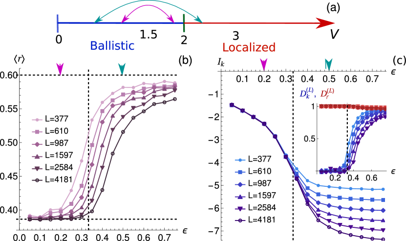
Figure 5: (a) Floquet-drive location on the static phase diagram of the Aubry-André model. The arrows indicate two amplitudes $\epsilon$ of quasiperiodic potentials used in the periodic quench for $V=1.5$, also shown in (b,c): quench between ballistic states (magenta); and quench between ballistic and localized states (cyan). (b) $\langle r\rangle$ for $V=1.5$ and $T=500$, as a function of $\epsilon$, for different system sizes $L$. The vertical dashed line indicates the value $\epsilon=\epsilon^{*}$ above which we start quenching ballistic and localized states, while the horizontal dashed lines indicate $r_{{\rm GUE}}$ (ergodic) and $r_{{\rm Poisson}}$. (c) $\mathcal{I}_{k}$ for the same parameters as in (b). The inset contains the real- and momentum-space finite-size fractal dimensions defined in Eq. (5).

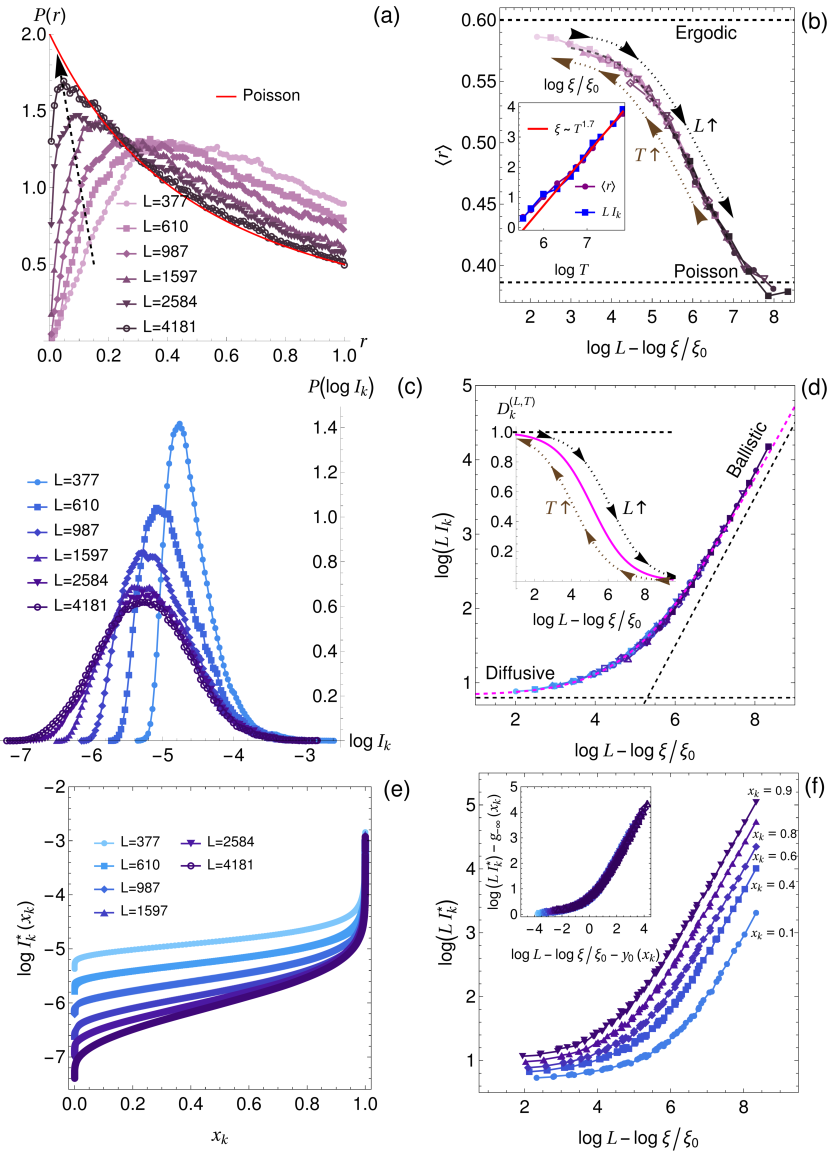
Figure 6: Quench’s center of mass in ballistic phase: Results for $V=1.5,\epsilon=0.375$. (a) $P(r)$ distribution for $T=400$, for different system sizes. The arrow points towards increasing $L$ and the full red line indicates the Poisson distribution $P(r)=2/(1+r)^{2}$. (b) Scaling collapses of $\langle r\rangle$ calculated for values of $T$ belonging to the interval $T\in[200,2500]$ and $L\in[377,4181]$. The correlation lengths $\xi$ were obtained from the scaling collapse and $\xi_{0}=\xi(T=200)$. The black (brown) arrows point towards increasing $L$ ($T$). The inset shows $\log(\xi/\xi_{0})$ as function of $\log T$, for both the collapses of $\langle r\rangle$ and of $L\mathcal{I}_{k}$ done in (d), yielding compatible results. The cyan line was obtained by fitting for the data points at $6$ largest $T$-values (combining the data from $\langle r\rangle$ and $L\mathcal{I}_{k}$ ), yielding a power-law $\xi\sim T^{1.7}$. (c) Distribution $P(\log\mathcal{I}_{k})$ for $T=400$ and different system sizes. (d) Scaling collapses of $L\mathcal{I}_{k}$. The large $L$ localized behaviour $L\mathcal{I}_{k}\sim L$ and large $\xi$ (or $T$) diffusive behaviour $L\mathcal{I}_{k}\sim L^{0}$ are indicated by the black dashed lines. We find that $\log(L\mathcal{I}_{k})$ is well fitted by the expression $g(y)=g_{-\infty}+\log(1+e^{y-y_{0}})$, where $y=\log L-\log\xi/\xi_{0}$, shown in the dashed magenta line. We obtain the fractal dimension from this fit through $D_{k}^{(L,T)}=1-[\log(L\mathcal{I}_{k})]^{\prime}$ and show in the inset, in full magenta. (e) $\log\mathcal{I}_{k}^{*}(x_{k})$, for different $L$ and for $T=850$. (f) Scaling collapses of $\log\mathcal{I}_{k}^{*}(x_{k})$ for different values of $x_{k}$ indicated in the figure. We note that the computed $\xi(x_{k})$ are identical for the different $x_{k}$, as shown in Fig. 8(b). By fitting the collapsed data for different $x_{k}$ to $g^{(x_{k})}(y)=g_{-\infty}(x_{k})+\log\left(1+e^{y-y_{0}(x_{k})}\right)$ we were able to collapse all the curves into an universal curve shown in the inset. The fitted parameters $g_{-\infty}(x_{k})$ and $y_{0}(x_{k})$ are plotted in Fig. 9(b).

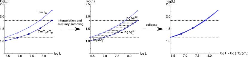
Figure 7: Method used for data collapse. We first interpolate the original data points, corresponding to a given $T=T_{0}$ and $T=T_{1}>T_{0}$ and uniformly sample $N_{p}$ points of the resulting function in the vertical region of overlap between the two functions (in our calculations we usually take $N_{p}=10$ and a linear interpolation). We then compute all the distances between the sampled points $\log\Delta\xi_{1}^{(i)},i=1,\cdots,N_{p}$ and define $\log\Delta\xi_{1}=N_{p}^{-1}\sum_{i}\log\Delta\xi_{1}^{(i)}$. We then use this distance to collapse the data. Considering $\xi_{0}$ to be the correlation length at $T=T_{0}$, we then have $\log\xi(T_{1})=\log\xi_{0}+\log\Delta\xi_{1}$. We can then iterate this procedure by taking larger periods $T_{n}$, always collapsing the curves for $T=T_{n}$ and $T=T_{n-1}$, from which $\log\Delta\xi_{n}$ can be extracted. We can then compute $\log[\xi(T=T_{n})/\xi_{0}]=\sum_{m=1}^{n}\log\Delta\xi_{m}$.

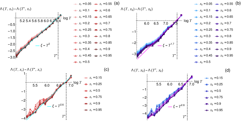
Figure 8: Plots of $\Lambda(T,x_{p})-\Lambda(T^{*},x_{p})$, where $\Lambda(T,x_{p})=\log[\xi(T,x_{p})/\xi_{0}(T,x_{p})]$, with $p=r,k$, and $\log T^{*}$ is indicated in the figures by the vertical dashed line. Note that the subtraction of $\Lambda(T^{*},x_{p})$ is just a trivial $x_{p}$-dependent vertical shift in $\log[\xi(T,x_{p})]$ that we applied to better see the identical slopes. (a) $V=3,\epsilon=0.45$, for collapses in Fig. 2(f). (b) $V=1.5,\epsilon=0.375$, for collapses in Fig. 6(f). (c,d) $V=2,\epsilon=0.2$, for collapses shown in Fig. 3(d). In all figures we show in cyan or magenta the power-laws obtained in the main text and Fig. 6, for comparison.

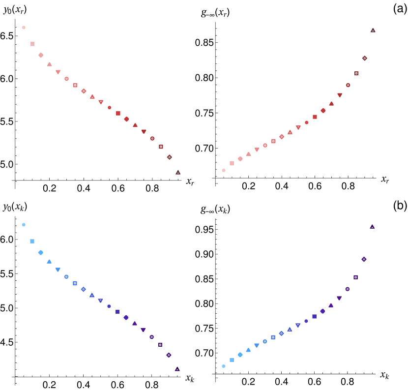
Figure 9: Parameters extracted from the fits to the expression $g^{(x_{p})}(y)=g_{-\infty}(x_{p})+\log(1+e^{y-y_{0}(x_{p})})$, with $p=r,k$, for the scaling collapses in (a) Fig. 2(f); (b) Fig. 6(f).

Appendix B Details on scaling collapses

In this section, we provide details on the scaling collapses carried out throughout the manuscript and present additional information extracted from these collapses.

The scaling collapse method is illustrated in Fig. 7 and described in detail in the figure’s caption. In Fig. 8, we show plots for $\xi(T,x_{p})$ ($p=r,k$) extracted from the $x_{p}$-dependent scaling collapses done in Figs. 2, 3, 6. We can see that in all cases, the results depend very weakly on $x_{p}$ for large enough $T$.

Finally, in Fig. 9, we plot the fitting parameters used for the scaling collapses for all $x_{p}$ in the insets of Fig. 2(f) and Fig. 6(f).

Appendix C Localization-delocalization transition in Ref.  (Sarkar et al., 2021)

In Ref. (Sarkar et al., 2021), a driven Aubry-André model was also studied, with a different driving protocol than the one studied here. The Hamiltonian in this study was given by

$$\begin{array}[]{cc}H(t)=&-J(t)/2\sum_{n}c_{n}^{\dagger}c_{n+1}+\textrm{h.c.}\\ &+\sum_{n}V\cos(2\pi\tau n+\phi)c_{n}^{\dagger}c_{n}\end{array}$$ (10)

where

$$J(t)=\begin{cases}-J_{0}&t\leq T/2\\ J_{0}&t>T/2\end{cases}.$$ (11)

and $T$ is the driving period, with corresponding driving frequency $\omega_{D}=2\pi/T$. Since in this case there is also a square-drive protocol, the Floquet Hamiltonian can be easily obtained as in Eq. (2) of the main text. In Fig 10, we study the localization properties of the Floquet Hamiltonian of the model in Eqs. (10), (11), for the same model parameters studied in Ref. (Sarkar et al., 2021). In Fig. 10(a), we can clearly see that all states are localized for large enough $\omega_{D}$ (region of large IPR), while extended states with small IPR arise at smaller $\omega_{D}$, as observed in Ref. (Sarkar et al., 2021). An important question is whether this extended region is ergodic, which would go against our conjecture that ergodicity is generically not robust in the thermodynamic limit, for driven non-interacting 1D quasiperiodic systems. However, supported by the results in Fig. 10(b), we find that the extended region is in fact a ballistic non-ergodic phase.

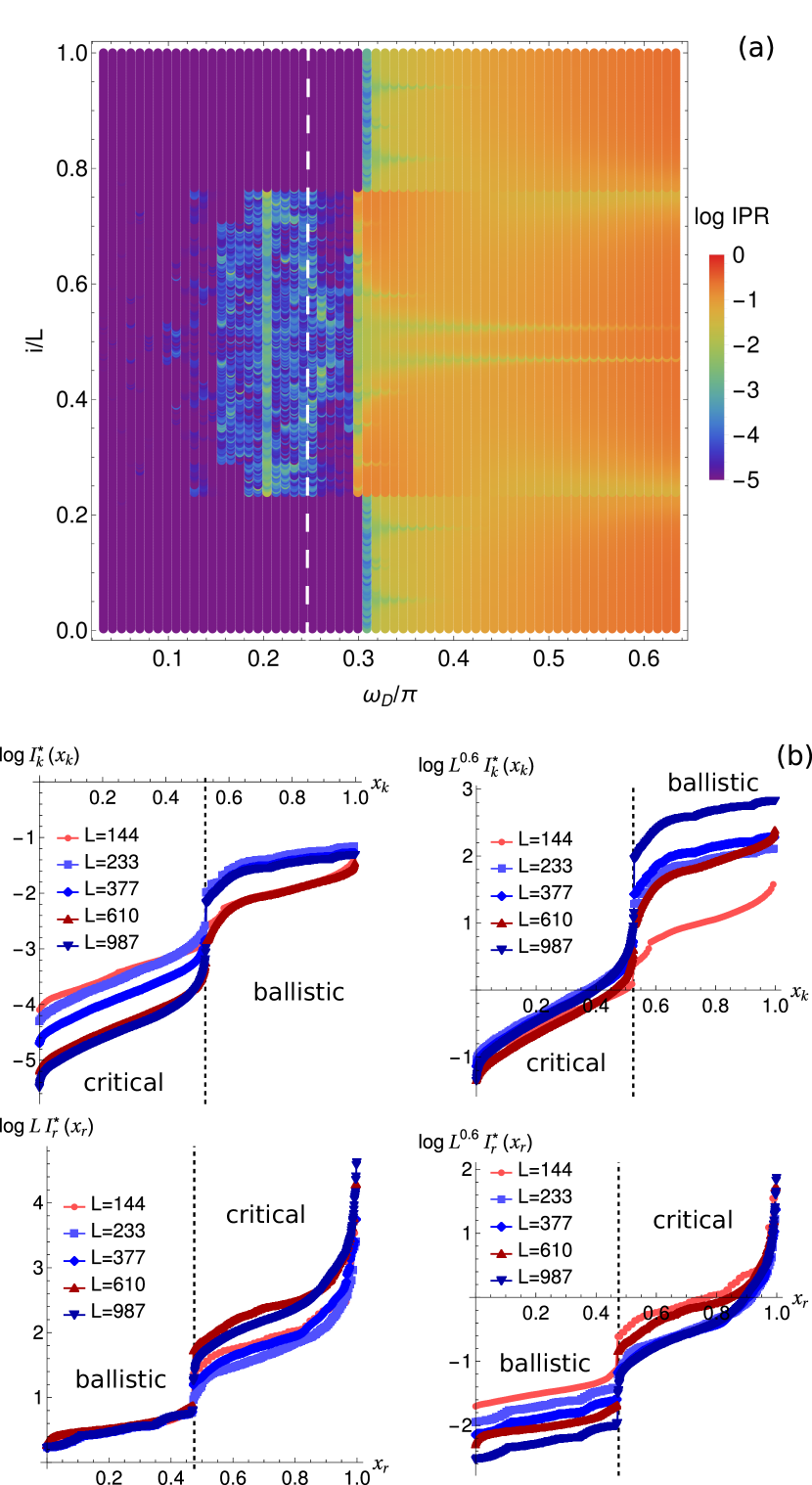
Figure 10: Results for the Floquet Hamiltonian of the model in Eqs. (10), (11) introduced in Ref. (Sarkar et al., 2021), for the same parameters studied there: $V/J_{0}=0.05$, $J_{0}=1$ and $\tau=(\sqrt{5}-1)/2$. As in the main text, we use approximant system sizes by choosing $L=F_{n}$ and $\tau=F_{n+1}/F_{n}$, where $F_{n}$ is the n-th Fibonacci number. (a) Color plot of the IPR for $L=144$ as a function of driving frequency $\omega_{D}$ and normalized eigenstate index $i/L$, for a random phase $\phi$ and twist $\kappa$. The eigenstates were ordered by increasing quasienergy in the interval $[-\pi,\pi[$. (b) $\mathcal{I}_{k}^{*}(x_{k})$ and $\mathcal{I}_{r}^{*}(x_{r})$ as defined in the main text, for $\omega_{D}=0.245\pi$ indicated in (a) (dashed white line). Up to different scaling functions for even (red points) and odd (blue points) sizes, we can clearly identify a ballistic and a critical regime. The former and the latter correspond respectively to the extended and multifractal regimes found in Ref. (Sarkar et al., 2021).