A Precise Electron EDM Constraint on CP-odd Heavy-Quark Yukawas

Abstract

CP-odd Higgs couplings to bottom and charm quarks arise in many extensions of the standard model and are of potential interest for electroweak baryogenesis. These couplings induce a contribution to the electron EDM. The experimental limit on the latter then leads to a strong bound on the CP-odd Higgs couplings. We point out that this bound receives large QCD corrections, even though it arises from a leptonic observable. We calculate the contribution of CP-odd Higgs couplings to the bottom and charm quarks in renormalisation-group improved perturbation theory at next-to-leading order in the strong interaction, thereby reducing the uncertainty to a few percent.

1 Introduction

The precise determination of the Yukawa couplings of the Higgs boson to all fermions has been a focus of particle physics since the discovery of the Higgs boson in 2012 [1, 2]. In the Standard Model (SM) all Yukawa couplings are aligned with the fermion masses and thus real, but multiple extensions of the SM induce non-trivial phases. This is of particular interest as these phases (mainly in the Yukawa couplings to the third fermion generation) play a leading role in models of electroweak baryogenesis [3]. In this article, we focus on the bottom- and charm-quark Yukawa couplings.

It is well-known that the present bounds on the electric dipole moment (EDM) of the electron place strong constraints on CP-violating phases in the quark Yukawa couplings [4, 5, 6, 7, 8]. However, it is less well-appreciated (and maybe somewhat surprising) that the heavy-quark contributions to the electron EDM receive large QCD corrections, leading to a large implicit uncertainty in the current constraints. In this section, we briefly review the current situation. In the remainder of this article, we calculate the leading logarithmic (LL) and next-to-leading logarithmic (NLL) QCD corrections, thereby reducing the presently ${\cal O}(1)$ uncertainty to a few percent.

For the purpose of this work, we assume a modification of the SM heavy-quark Yukawa couplings of the form

$$\mathscr{L}_{h{q_{h}}{q_{h}}}=-\frac{y^{\text{SM}}_{q_{h}}}{\sqrt{2}}\kappa_{q_{h}}{\bar{q}_{h}}\left(\cos\phi_{q_{h}}+i\gamma_{5}\sin\phi_{q_{h}}\right){q_{h}}\,h\,.$$ (1)

Here, ${q_{h}}=b,c$ denotes the bottom- or charm-quark field and $h$ the physical Higgs field. Moreover, $y^{\text{SM}}_{q_{h}}\equiv m_{q_{h}}e/\sqrt{2}s_{w}M_{W}$ is the SM Yukawa, with $e$ the positron charge, $s_{w}$ the sine of the weak mixing angle, and $m_{q}$ and $M_{W}$ the heavy-quark and $W$-boson masses, respectively. The real parameter $\kappa_{q_{h}}\geq 0$ parameterises modifications to the absolute value of the Yukawa coupling, while the phase $\phi_{q_{h}}\in[0,2\pi)$ parameterises CP violation. The SM corresponds to the values $\kappa_{q_{h}}=1$ and $\phi_{q_{h}}=0$.

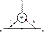
Figure 1: Barr–Zee diagram that contributes to the electron EDM from a CP-odd heavy-quark Yukawa coupling with the Higgs (red square).

Virtual heavy quarks with CP-odd Higgs couplings induce an electron EDM $d_{e}$, defined by

$$\mathscr{L}_{\mathrm{e}ff}=-d_{e}\,\frac{i}{2}\,\bar{e}\sigma^{\mu\nu}\gamma_{5}e\,F_{\mu\nu}\,,$$ (2)

with $\sigma^{\mu\nu}\equiv\tfrac{i}{2}[\gamma^{\mu},\gamma^{\nu}]$, via the well-known Barr–Zee diagrams [11]. Calculating the two-loop Barr–Zee diagrams (see Figure 1) keeping the non-zero heavy-quark mass and expanding the loop functions for small quark mass and small external momenta leads to [4]

$$\begin{split}d_{e}&\simeq-12eQ_{e}Q_{q_{h}}^{2}\,\frac{\alpha_{e}}{(4\pi)^{3}}\sqrt{2}G_{F}m_{e}\,\kappa_{q_{h}}\sin\phi_{q_{h}}\,x_{q_{h}}\left(\log^{2}x_{q_{h}}+\frac{\pi^{2}}{3}\right)\,,\end{split}$$ (3)

up to higher orders in the ratio $x_{q_{h}}\equiv m_{q_{h}}^{2}/M_{h}^{2}$ (with $M_{h}\sim 125\,$GeV the Higgs-boson mass). Here, $\alpha_{e}$ is the fine-structure constant, $Q_{q_{h}}$ is the charge of the heavy quark with $Q_{b}=-1/3$ and $Q_{c}=+2/3$, and $Q_{e}=-1$ is the electron charge. Barr–Zee diagrams with an internal $Z$ boson also affect the electron EDM, however, they lead to a contribution that is suppressed with respect to those with an internal photon by the small coupling of the $Z$ boson to electrons [4].

Using the ACME result, $|d_{e}|<1.1\times 10^{-29}\,e\,\text{cm}$ (at 90% CL)  [12], Eq. (3) implies the bounds $\kappa_{b}|\sin\phi_{b}|\leq 0.41$ and $\kappa_{c}|\sin\phi_{c}|\leq 1.1$ at the 90% CL for the bottom- and charm-quark case, respectively. However, to obtain these bounds, numerical values for the heavy-quark masses must be chosen. It is not clear a priori at which scale the quark masses should be evaluated; $\mu=M_{h}$ and $\mu=m_{q_{h}}$ would be obvious choices. For the bounds above, we used the values $m_{b}(M_{h})$ and $m_{c}(M_{h})$; choosing $m_{b}(m_{b})$ and $m_{c}(m_{c})$ instead leads to the significantly stronger bounds $\kappa_{b}|\sin\phi_{b}|\leq 0.23$ and $\kappa_{c}|\sin\phi_{c}|\leq 0.35$ at the 90% CL. The differences arise from the large QCD running of the quark masses between the two scales $\mu=M_{h}$ and $\mu=m_{q_{h}}$. This indicates that the QCD corrections to Eq. (3) are large, even though the electron EDM is a leptonic observable. By our explicit calculation, we will show that the predicted value for $d_{e}$ after resolving the ambiguity lies somewhere in between the values obtained by using the two scales $M_{h}$ and $m_{q_{h}}$.

We give here a brief outline of the main ideas of the calculation. First, notice that the result in Eq. (3), which was obtained by a two-loop, fixed-order calculation, is numerically dominated by the large quadratic logarithms $\log^{2}x_{q_{h}}$. This logarithmic contribution can be reproduced by the one-loop QED renormalisation-group (RG) evolution in an appropriate effective theory (see Section 2), truncated at order $\alpha_{e}^{2}$. The second term in Eq. (3), $\pi^{2}/3$, has no logarithmic dependence on the mass ratio and is formally of next-to-next-to-leading-logarithmic (NNLL) order in RG-improved perturbation theory. Numerically, this term gives a $\sim 6\%$ correction to the logarithmic contribution to $d_{e}/e$ in the bottom case and a $\sim 3.5\%$ correction in the charm case. On the other hand, we have seen above that the choice of different renormalisation scales for the quark masses represents a much larger uncertainty, of the order of $100\%$.

We, thus, conclude that the QCD corrections to the Barr–Zee diagrams are large, and we expect that these corrections are dominated by leading QCD logarithms, since the product $\alpha_{s}\log x_{q_{h}}$ is large ($\alpha_{s}$ denotes the strong coupling constant). These logarithms can be reliably calculated using RG-improved perturbation theory. The result with resummed leading QCD logarithms has the schematic form $\alpha_{e}^{2}\log^{2}x_{q_{h}}(1+\alpha_{s}\log x_{q_{h}}+\alpha_{s}^{2}\log^{2}x_{q_{h}}+\ldots)$. Here, the first term reflects the quadratic logarithm in Eq. (3), while all other terms correspond to the leading logarithms of the diagrams obtained by dressing the Barr-Zee diagrams, Figure 1, with an arbitrary number of gluons.

It is, however, well-known that one can only consistently fix the scale and scheme dependence of the input parameters by going beyond the LL approximation. Hence, we will also perform the NLL calculation, reducing the the uncertainty down to the percent level. This corresponds roughly to the size of the correction that we have estimated above using the $\pi^{2}/3$ term in the fixed-order result, which can be viewed as part of the NNLL order result in RG-improved perturbation theory. This term is thus not included in our NLL calculation.

Our calculation will show that the QCD perturbation series converges well, as might be expected for a leptonic observable. In addition, we emphasize that this is a complete calculation – no further hadronic input (such as the lattice matrix elements required for hadronic EDMs) is needed. The final result for $d_{e}/e$ lies between the two values obtained from the naive computation, determining the heavy quark masses at the different scales. All these results are illustrated in Figure 4 of Section 4.

This paper is organised as follows: in Section 2, we introduce the effective theories used in the computation. In Section 3, we present the detailed results of our calculation, namely, the initial conditions at the electroweak scale, the calculation of the anomalous dimensions, and the threshold corrections at the heavy-quark thresholds. We also show the final analytical results in a compact form. In Section 4, we present the numerical results of the calculation including updated bounds on the CP-odd heavy-quark Yukawa couplings. We conclude in Section 5. Additional information is presented in two appendices: In App. A, we collect the unphysical operators used in the computation of the anomalous-dimension matrix and in App. B, we show the results for renormalisation constants entering the calculation.

2 Effective Theories Below the Weak Scale

A precise determination of the electron EDM in the presence of CP-odd Higgs couplings to the bottom and charm quarks requires an effective field theory that allows to sum large QCD logarithms to all orders in the strong coupling constant and includes the effect of the combined $\alpha_{s}$ and $\alpha_{e}$ RG evolution. Based on the “full” Lagrangian in Eq. (1), we construct the effective Lagrangian below the electroweak scale, $\mu_{\text{ew}}$, by integrating out the heavy degrees of freedom of the SM (the top quark, the weak gauge bosons, and the Higgs). EDMs are then induced by non-renormalisable operators that are CP odd. In the current work, we focus on the part of the effective Lagrangian that is relevant for predicting the electron EDM in the presence of CP-odd Yukawas couplings to the bottom and charm quarks. In this case, the relevant effective Lagrangian reads

$$\mathscr{L}_{\text{eff},{q_{h}}}=-\sqrt{2}G_{\mathrm{F}}\,\Big{(}C_{1}^{e{q_{h}}}O_{1}^{e{q_{h}}}+C_{1}^{{q_{h}}e}O_{1}^{{q_{h}}e}+C_{2}^{e{q_{h}}}O_{2}^{e{q_{h}}}+C_{3}^{e}O_{3}^{e}\Big{)}+\ldots\,,$$ (4)

where the four linearly independent operators are

$$O_{1}^{e{q_{h}}} =(\bar{e}e)\,({\bar{q}_{h}}\,i\gamma_{5}{q_{h}})\,, O_{1}^{{q_{h}}e} =({\bar{q}_{h}}{q_{h}})\,(\bar{e}\,i\gamma_{5}e)\,,$$

$$O_{2}^{e{q_{h}}} =\frac{1}{2}\epsilon^{\mu\nu\rho\sigma}(\bar{e}\sigma_{\mu\nu}e)\,({\bar{q}_{h}}\,\sigma_{\rho\sigma}{q_{h}})\,, O_{3}^{e} =\frac{Q_{e}}{2}\frac{m_{q_{h}}}{e}\,(\bar{e}\sigma^{\mu\nu}e)\,\tilde{F}_{\mu\nu}\,,$$ (5)

and $C_{1}^{e{q_{h}}}$, $C_{1}^{{q_{h}}e}$, $C_{2}^{e{q_{h}}}$, and $C_{3}^{e}$ are the corresponding Wilson coefficients. Additional CP-odd operators that are suppressed by additional factors of $m_{\text{light}}/m_{q_{h}}$ (where $m_{\text{light}}$ corresponds to a light quark mass) are denoted by the ellipsis. We defined the electron dipole operator with a factor of the running quark mass $m_{q_{h}}\equiv m_{q_{h}}(\mu)$, to avoid awkward ratios of quark and lepton masses in the anomalous dimensions. Throughout this work the $\gamma_{5}$ matrix is defined by

$$\gamma_{5}\equiv\frac{i}{4!}\epsilon_{\mu\nu\rho\sigma}\gamma^{\mu}\gamma^{\nu}\gamma^{\rho}\gamma^{\sigma}\,,$$ (6)

where $\epsilon^{\mu\nu\rho\sigma}$ is the totally antisymmetric Levi-Civita tensor in four space-time dimensions with $\epsilon_{0123}=-\epsilon^{0123}=1$, and we use the notation $\widetilde{F}^{\mu\nu}=\tfrac{1}{2}\epsilon^{\mu\nu\rho\sigma}F_{\rho\sigma}$. We treat $\gamma_{5}$ within the “Larin” scheme; for the details and subtleties we refer to Ref. [6]. The non-standard sign convention for $O_{3}^{q}$ is related to our definition of the covariant derivative acting on fermion fields $f$,

$$D_{\mu}\equiv\partial_{\mu}-ig_{s}T^{a}G_{\mu}^{a}+ieQ_{f}A_{\mu}\,.$$ (7)

The basis of all flavour-diagonal, CP-odd operators is closed under the QED and QCD RG flow, as both interactions conserve CP and flavour. Below the electroweak scale, there is a tower of effective theories relevant for predicting the electron EDM. For the bottom case, ${q_{h}}=b$, we employ the effective Lagrangian in Eq. (4) for the five-flavour theory, while for the charm case, ${q_{h}}=c$, we employ Eq. (4) for both the five-flavour and the four-flavour theory (see discussion in Section 3.3 for the threshold corrections on couplings and Wilson coefficients at the bottom-quark scale).

The effective theory below the heavy-quark scale, $\mu_{{q_{h}}}$, does not contain four-fermion operators with heavy quarks, and we use the modified effective Lagrangian

$$\widetilde{\mathscr{L}}_{\text{eff},{q_{h}}}=-\sqrt{2}G_{\mathrm{F}}\widetilde{C}_{3}^{e}\widetilde{O}_{3}^{e}+\ldots\,,$$ (8)

in which – as opposed to Eq. (4) – the dipole operator is defined with the conventional factor $m_{e}$:

$$\widetilde{O}_{3}^{e}=\frac{Q_{e}}{2}\frac{m_{e}}{e}\,(\bar{e}\sigma^{\mu\nu}e)\,\tilde{F}_{\mu\nu}\,.$$ (9)

Note that for ${q_{h}}=b$ the Lagrangian in Eq. (8) refers to the four-flavour Lagrangian, while for ${q_{h}}=c$ to the three-flavour one. This definition of $\widetilde{\mathscr{L}}_{\text{eff},{q_{h}}}$ implies that (cf. Eq. (2))

$$\frac{d_{e}}{e}=-\sqrt{2}G_{\mathrm{F}}\frac{m_{e}}{4\pi\alpha_{e}}\widetilde{C}_{3}^{e}\,.$$ (10)

In the next section, we describe how the RG evolution within the effective field theories relates $d_{e}$ to the parameters $\kappa_{q_{h}}$ and $\phi_{q_{h}}$ of the “full” theory in Eq. (1).

3 Renormalisation Group Evolution

Our goal is the summation of all leading and next-to-leading logarithms via RG-improved perturbation theory. The calculation proceeds in the following steps.

First, we integrate out the Higgs and weak gauge bosons together with the top quark at the electroweak scale, $\mu_{\text{ew}}\sim M_{h}$. This matching calculation at $\mu_{\text{ew}}$ induces the initial conditions for the five-flavour Wilson coefficients appearing in Eq. (4). We collect them in Section 3.1. Subsequently, we perform the RG evolution from $\mu_{\text{ew}}$ down to the bottom-quark threshold, $\mu_{b}\sim m_{b}(m_{b})$. The anomalous dimensions relevant for the mixed QCD–QED RG evolution at NLL accuracy are computed here for the first time, see Section 3.2. The next step depends on whether ${q_{h}}=b$ or ${q_{h}}=c$. For the bottom case, ${q_{h}}=b$, we match directly to the four-flavour version of the Lagrangian in Eq. (8) to obtain the prediction of the electron EDM. The relevant threshold corrections at $\mu_{b}$ are discussed in Section 3.3. For the charm case, ${q_{h}}=c$, we must instead match at $\mu_{b}$ to the four-flavour version of the Lagrangian with four-fermion operators in Eq. (4) and additionally perform the RG evolution in the four-flavour theory from $\mu_{b}$ down to $\mu_{c}\sim m_{c}(m_{c})$. The corresponding anomalous dimensions are also given in section 3.2. Finally, we match to the three-flavour version of the Lagrangian in Eq. (8) to obtain the prediction of the electron EDM.

The calculations of the amplitudes relevant for computing the initial conditions of Wilson coefficients and the hitherto unknown anomalous dimensions have been performed with self-written FORM [13] routines, i.e., MaRTIn [14], implementing the two-loop recursion algorithms presented in Refs. [15, 16]. The amplitudes were generated using QGRAF [17].

The RG evolution between the different matching scales is significantly more involved than in applications in which the electromagnetic coupling, $\alpha_{e}$, can be neglected. The reason is that the leading contribution to the electron EDM contains a term with two powers of the large logarithm, i.e, $\log^{2}x_{q_{h}}$, see Eq. (3). Within the effective theory, this term is obtained by a LL QED calculation, truncated at order $\alpha_{e}^{2}$. However, the numerically relevant corrections to this result are not further electromagnetic $\alpha_{e}^{n}\log^{n}$ corrections, but large, logarithmically enhanced QCD corrections which must be summed to all orders to obtain an accurate prediction. Therefore, to properly account for the numerically relevant corrections we must consistently solve the mixed QCD–QED RG equations.

This can be achieved consistently using the general formalism developed in Ref. [18]. The main idea is that, since $\alpha_{s}\log x_{q_{h}}$ is ${\cal O}(1)$, such products of QCD coupling times large logarithms must be resummed for an accurate prediction. By contrast, the product $\alpha_{e}\log x_{q_{h}}$ is small and does not require resummation. The large logarithms appearing in $\alpha_{e}\log x_{q_{h}}$ are expressed in terms of the resummed $\alpha_{s}\log x_{q_{h}}$, i.e. $\alpha_{e}\log x_{q_{h}}=(\alpha_{e}/\alpha_{s})\times\alpha_{s}\log x_{q_{h}}$. As a consequence, the conventional expansion in terms of $\alpha_{s}$ and $\alpha_{e}$ is replaced by an expansion in $\alpha_{s}$ and $\kappa\equiv\alpha_{e}/\alpha_{s}$. Therefore, in this setup the Wilson coefficients at some scale $\mu$ have the expansion

$$C_{i}(\mu)=\sum_{n,m=0}^{\infty}\tilde{\alpha}_{s}(\mu)^{n}\kappa(\mu)^{m}\,C^{(nm)}_{i}(\mu)\,,$$ (11)

with $\tilde{\alpha}_{s}\equiv\alpha_{s}/4\pi$. By implementing the mixed RG evolution we will compute the $C^{(nm)}_{i}(\mu)$ coefficients relevant for the electron EDM; for details we refer to Ref. [18]. The analytical results are presented in Section 3.4.

3.1 Initial Conditions at the Weak Scale

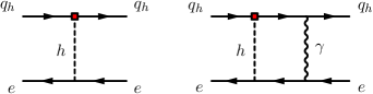
Figure 2: Examples of leading order (left) and next-to-leading order (right) Feynman diagrams that contribute to the initial conditions of the four-fermion sector in the EFT. CP-odd heavy-quark Yukawa couplings are indicated by red squares.

We augment the SM by flavour-conserving, CP-odd Higgs Yukawa couplings to the heavy quarks ${q_{h}}=b,c$, as parameterised in Eq. (1). At a scale $\mu_{\text{ew}}\approx M_{h}$ we integrate out the heavy degrees of freedom of the SM and match to the effective five-flavour theory relevant for the electron EDM in Eq. (4). The initial conditions for the Wilson coefficients relevant for our calculation are obtained by evaluating the tree-level and one-loop Feynman diagrams such as those shown in Figure 2; we find

$$C_{1}^{e{q_{h}}}(\mu_{\text{ew}}) =-\kappa_{q_{h}}\sin\phi_{q_{h}}\frac{m_{e}m_{{q_{h}}}}{M_{h}^{2}}+{\cal O}(\alpha_{s}^{2},\alpha_{s}\alpha_{e},\alpha_{e}^{2})\,,$$ (12)

$$C_{1}^{{q_{h}}e}(\mu_{\text{ew}}) =0+{\cal O}(\alpha_{s}^{2},\alpha_{s}\alpha_{e},\alpha_{e}^{2})\,,$$ (13)

$$\begin{split}C_{2}^{e{q_{h}}}(\mu_{\text{ew}})&=\frac{\alpha_{e}}{4\pi}\left(\frac{3}{2}+\log\frac{\mu_{\text{ew}}^{2}}{M_{h}^{2}}\right)\frac{m_{e}m_{{q_{h}}}}{M_{h}^{2}}Q_{e}Q_{q_{h}}\kappa_{q_{h}}\sin\phi_{q_{h}}+{\cal O}(\alpha_{s}^{2},\alpha_{s}\alpha_{e},\alpha_{e}^{2})\,,\end{split}$$ (14)

$$C_{3}^{e}(\mu_{\text{ew}}) =0+{\cal O}(\alpha_{e}^{2})\,.$$ (15)

All parameters appearing above correspond to parameters in the five-flavour theory evaluated at the scale $\mu_{\text{ew}}$, i.e., $m_{q_{h}}=m_{{q_{h}},\text{5fl}}(\mu_{\text{ew}})$ and $\alpha_{e}=\alpha_{e,\text{5fl}}(\mu_{\text{ew}})$. We treat the heavy quarks and the electron as massless at the electroweak matching scale; therefore, no powers of $m_{e}/M_{h}$ or $m_{q_{h}}/M_{h}$ appear in the results. The explicit factors of the electron and heavy-quark masses arise by expressing the Yukawa couplings in Eq. (1) in terms of $m_{e}$ and $m_{q_{h}}$. We have included all terms up to corrections of quadratic order in the strong and electromagnetic coupling constants, as only these are required for our analysis. The ${\mathcal{O}}(\alpha_{e})$ coefficient, Eq. (14), is well-defined only after specifying the basis of evanescent operators which can be found in App. A.

In Section 3.4, we will use the framework of Ref. [18] to solve the mixed QCD–QED RG as an expansion in $\tilde{\alpha}_{s}$ and $\kappa$. Based on Eqs. (12)-(14) we find the contributing expansion coefficients in Eq. (11)

$$\begin{split}C_{1}^{e{q_{h}},(00)}(\mu_{\text{ew}})&=-\kappa_{q_{h}}\sin\phi_{q_{h}}\frac{m_{e}m_{{q_{h}}}}{M_{h}^{2}}\,,\\ C_{2}^{e{q_{h}},(11)}(\mu_{\text{ew}})&=\left(\frac{3}{2}+\log\frac{\mu_{\text{ew}}^{2}}{M_{h}^{2}}\right)\frac{m_{e}m_{{q_{h}}}}{M_{h}^{2}}Q_{e}Q_{q_{h}}\kappa_{q_{h}}\sin\phi_{q_{h}}\,.\end{split}$$ (16)

3.2 Anomalous Dimensions

To solve the RG in the effective theories below the electroweak scale we need to include the running of coupling constants, mass anomalous dimensions, and the mixing of operators. In this section, we collect the results that enter the analysis at NLL accuracy.

The running of the Wilson coefficients from the electroweak matching scale down to the relevant quark scale is governed by the RG equation

$$\frac{dC_{i}}{d\log\mu}=C_{j}\gamma_{ji}\,,$$ (17)

where $\gamma_{ji}$ are the components of the anomalous dimension matrix (ADM). We choose the ordering of Wilson coefficients as

$$\vec{C}=(C_{1}^{e{q_{h}}},~{}C_{1}^{{q_{h}}e},~{}C_{2}^{e{q_{h}}},~{}C_{3}^{e})^{T}\,.$$ (18)

The ADM admits an expansion in powers of $\tilde{\alpha}_{s}\equiv\alpha_{s}/4\pi$ and $\tilde{\alpha}_{e}\equiv\alpha_{e}/4\pi$,

$$\gamma=\sum_{\begin{subarray}{c}n,m=0\\ n+m\geq 1\end{subarray}}\gamma^{(nm)}\tilde{\alpha}_{s}(\mu)^{n}\tilde{\alpha}_{e}(\mu)^{m}\,,$$ (19)

with $\tilde{\alpha}_{s}$, $\tilde{\alpha}_{e}$, and $\gamma^{(nm)}$ depending on the number of active fermion flavours in the effective theory. Using this expansion, the ADM can be organised by loop order. In general, it depends on the number of active fermion flavours and on the flavour of the heavy quark ${q_{h}}$. Below we present our results entering the five- and four-flavour RG evolution required for the case ${q_{h}}=b$ and ${q_{h}}=c$.

By explicit calculation, we find at one loop

$$\gamma^{(01)} =\begin{pmatrix}-6(Q_{e}^{2}+Q_{q_{h}}^{2})&0&-2Q_{e}Q_{q_{h}}&0\\[5.0pt] 0&-6(Q_{e}^{2}+Q_{q_{h}}^{2})&-2Q_{e}Q_{q_{h}}&0\\[5.0pt] -48Q_{q_{h}}Q_{e}&-48Q_{q_{h}}Q_{e}&2(Q_{e}^{2}+Q_{q_{h}}^{2})&-48\frac{Q_{q_{h}}}{Q_{e}}\\[5.0pt] 0&0&0&10Q_{e}^{2}+6Q_{q_{h}}^{2}-2\beta_{e}^{(0)}\end{pmatrix}\,,$$ (20)

$$\gamma^{(10)} =\begin{pmatrix}-6C_{F}&0&0&0\\[5.0pt] 0&-6C_{F}&0&0\\[5.0pt] 0&0&2C_{F}&0\\[5.0pt] 0&0&0&\gamma_{{q_{h}},s}^{(0)}\end{pmatrix}\,,$$ (21)

with $\beta_{e}^{(0)}=-\frac{4}{3}\Big{(}N_{c}n_{d}Q_{b}^{2}+N_{c}n_{u}Q_{c}^{2}+n_{\ell}Q_{e}^{2}\Big{)}$ and $\gamma_{{q_{h}},s}^{(0)}=6C_{F}$. Moreover, $N_{c}=3$ is the number of quark colors, $n_{u}$ is the number of active up-type quarks, $n_{d}$ is the number of active down-type quarks, $n_{\ell}$ is the number of active charged leptons and $C_{F}\equiv(N_{c}^{2}-1)/2N_{c}=4/3$. In both the bottom and charm cases, we have $n_{u}=2$ and $n_{\ell}=3$.

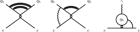
Figure 3: Examples of two-loop QCD (left), mixed QED–QCD (middle), and two-loop QED (right) Feynman diagrams entering the computation of the anomalous dimension matrix. Effective operator insertions are represented by the unshaded boxes.

At two-loop, the pure QCD ADM is the same for the bottom- and charm-quark case and depends on the number of active quark flavours,

$$\gamma^{(20)}=\begin{pmatrix}\frac{724}{9}-\frac{88n_{d}}{9}&0&0&0\\[5.0pt] 0&-\frac{1132}{9}+\frac{40n_{d}}{9}&0&0\\[5.0pt] 0&0&\frac{1964}{27}-\frac{104n_{d}}{27}&0\\[5.0pt] 0&0&0&\frac{1132}{9}-\frac{40n_{d}}{9}\end{pmatrix}\,.$$ (22)

For the bottom case, we only need the five-flavour theory, i.e., we always fix $n_{d}=3$. For the charm case, we must solve the RG in both five- and four-flavour theory in which case $n_{d}=3$ and $n_{d}=2$, respectively.

For the two-loop mixed QCD–QED and the pure two-loop QED ADMs, explicit factors of the quark charges result in different results for the bottom and charm cases. For notational simplicity, we quote the ADMs for the two cases separately after having substituted the electric charges. For the bottom, we find, after fixing $n_{d}=3$

$$\gamma^{(11)}_{[{q_{h}}=b]}=\begin{pmatrix}-\frac{8}{9}&0&-\frac{16}{9}&0\\[5.0pt] 0&-\frac{8}{9}&\frac{16}{3}&0\\[5.0pt] 128&-\frac{128}{3}&-\frac{152}{27}&-\frac{448}{3}\\[5.0pt] 0&0&0&40\end{pmatrix}\,,\quad\gamma^{(02)}_{[{q_{h}}=b]}=\begin{pmatrix}\frac{2420}{81}&-\frac{14}{3}&\frac{392}{81}&-8\\[5.0pt] -\frac{14}{3}&-\frac{7820}{81}&\frac{8}{81}&-\frac{8}{3}\\[5.0pt] \frac{64}{27}&\frac{3136}{27}&-\frac{17234}{243}&\frac{464}{9}\\[5.0pt] 0&0&0&-\frac{8704}{81}\end{pmatrix}\,.$$ (23)

For the charm, we find, keeping the $n_{d}$-dependence explicit

$$\gamma^{(11)}_{[{q_{h}}=c]} =\begin{pmatrix}-\frac{32}{9}&0&\frac{32}{9}&0\\[5.0pt] 0&-\frac{32}{9}&-\frac{32}{3}&0\\[5.0pt] -256&\frac{256}{3}&-\frac{608}{27}&\frac{896}{3}\\[5.0pt] 0&0&0&32+\frac{32n_{d}}{9}\end{pmatrix}\,,$$ (24)

$$\gamma^{(02)}_{[{q_{h}}=c]} =\begin{pmatrix}-\frac{439}{81}+\frac{4n_{d}}{81}&-\frac{56}{3}&-\frac{688}{81}-\frac{8n_{d}}{81}&-32\\[5.0pt] -\frac{56}{3}&-\frac{5879}{81}-\frac{316n_{d}}{81}&-\frac{208}{81}-\frac{8n_{d}}{81}&-\frac{32}{3}\\[5.0pt] -\frac{1664}{27}-\frac{64n_{d}}{27}&-\frac{5504}{27}-\frac{64n_{d}}{27}&-\frac{25661}{243}-\frac{676n_{d}}{243}&-\frac{256}{9}\\[5.0pt] 0&0&0&-\frac{8647}{81}-\frac{404n_{d}}{81}\end{pmatrix}\,.$$ (25)

Some representative Feynman diagrams used to compute the two-loop ADMs are shown in Figure 3. The two-loop ADM are well-defined only after specifying the basis of evanescent operators; this is done in App. A.

All two-loop results in this section are new, to the best of our knowledge. The one-loop RG evolution has also been calculated in Ref. [19].

3.3 Threshold Corrections

When performing the running of the Wilson coefficients, we must also integrate out the heavy quarks at the respective scales. This leads to threshold corrections to the gauge couplings and quark masses, as well as to the Wilson coefficients. Below we describe the origin of the threshold corrections for each case, and collect the corresponding results. Due to the mixed RG evolution, the matching of the effective theories must also be performed as an expansion in $\tilde{\alpha}_{s}$ and $\kappa$, cf. Eq. (11). We stress that the results presented below are only applicable for our specific case in which the only non-vanishing initial conditions are the ones in section 3.1. Other UV completions, with more contributions to the initial conditions, can receive additional threshold corrections (for instance, if $C^{e}_{3}(\mu_{\text{ew}})\neq 0$ at one-loop).

The Bottom-Quark Case

In the case of an anomalous bottom-quark Yukawa coupling, ${q_{h}}=b$, the only relevant threshold below the weak scale is at $\mu_{b}$ in which we match the five-flavour version of the Lagrangian in Eq. (4) to the four-flavour version of the Lagrangian in Eq. (8). There are three effects that induce a non-trivial correction to the matching onto $\widetilde{C}_{3}^{e}$: the threshold correction for $\alpha_{s}$ when matching from the five-flavour onto the four-flavour theories (the corresponding one for $\alpha_{e}$ does not contribute because in our case $C_{3,\text{5fl}}^{e,(01)}(\mu_{b})=0$); the different normalization of the dipole operators $O^{e}_{3}$ and $\widetilde{O}^{e}_{3}$ in the two theories, which leads to a factor of $m_{b}/m_{e}$; and a threshold correction from one-loop insertions of $O^{be}_{2}$ in the five-flavour theory. Details can be found in the analogous discussion in Ref. [6].

Taking all of these effects into account, we find for the electron dipole operator in the four-flavour theory at $\mu_{b}$

$$\widetilde{C}_{3}^{e}(\mu_{b})= \kappa_{\text{4fl}}^{2}\frac{m_{b}}{m_{e}}C_{3,\text{5fl}}^{e,(02)}(\mu_{b})$$

$$+ {\tilde{\alpha}_{s,\text{4fl}}}\kappa_{\text{4fl}}^{2}\frac{m_{b}}{m_{e}}\biggl{(}C_{3,\text{5fl}}^{e,(12)}(\mu_{b})+24\frac{Q_{b}}{Q_{e}}\log\frac{\mu_{b}^{2}}{m_{b}^{2}}C_{2,\text{5fl}}^{be,(01)}(\mu_{b})$$

$$\qquad\qquad\qquad\qquad-\frac{1}{2}\gamma_{b,s}^{(0)}\log\frac{\mu_{b}^{2}}{m_{b}^{2}}C_{3,\text{5fl}}^{e,(02)}(\mu_{b})-2\delta\alpha_{s}\log\frac{\mu_{b}^{2}}{m_{b}^{2}}C_{3,\text{5fl}}^{e,(02)}(\mu_{b})\biggr{)}$$ (26)

$$= \kappa_{\text{4fl}}^{2}\frac{m_{b}}{m_{e}}C_{3,\text{5fl}}^{e,(02)}(\mu_{b})$$

$$+ {\tilde{\alpha}_{s,\text{4fl}}}\kappa_{\text{4fl}}^{2}\frac{m_{b}}{m_{e}}\biggl{(}C_{3,\text{5fl}}^{e,(12)}(\mu_{b})+8\log\frac{\mu_{b}^{2}}{m_{b}^{2}}C_{2,\text{5fl}}^{be,(01)}(\mu_{b})-\frac{16}{3}\log\frac{\mu_{b}^{2}}{m_{b}^{2}}C_{3,\text{5fl}}^{e,(02)}(\mu_{b})\biggr{)}\,,$$ (27)

with $\gamma_{b,s}^{0}=6C_{F}$ the leading-order QCD mass anomalous dimension, the $\alpha_{s}$ threshold correction $\delta\alpha_{s}=2/3$, and $m_{b}=m_{b}(m_{b})$ in the five-flavour theory in the $\overline{\text{MS}}$ scheme. We indicate by explicit subscripts “5fl” and “4fl” in which effective theory the various quantities are defined. The couplings in Eq. (27) are evaluated at $\mu_{b}$, i.e., $\tilde{\alpha}_{s,\text{4fl}}(\mu_{b})$ and $\kappa_{\text{4fl}}(\mu_{b})$.

The Charm-Quark Case

In the case of an anomalous charm-quark Yukawa coupling, ${q_{h}}=b$, there are threshold corrections both at the bottom- and the charm-quark thresholds, $\mu_{b}$ and $\mu_{c}$, respectively.

At $\mu_{b}$, the effective Lagrangian in the five- and four-flavour theories are the same (see Eq. (4)), and at NLL accuracy the only relevant effect is the decoupling of $\alpha_{s}$. The only non-trivial matching condition at the bottom-quark scale then reads for the charm-quark case, ${q_{h}}=c$,

$$C_{3,\text{4fl}}^{e}(\mu_{b})=\kappa_{\text{4fl}}^{2}C_{3,\text{5fl}}^{e,(02)}(\mu_{b})+\tilde{\alpha}_{s,\text{4fl}}\kappa_{\text{4fl}}^{2}\biggl{(}C_{3,\text{5fl}}^{e,(12)}(\mu_{b})-2\delta\alpha_{s}\log\frac{\mu_{b}^{2}}{m_{b}^{2}}C_{3,\text{5fl}}^{e,(02)}(\mu_{b})\biggr{)}\,.$$ (28)

Other operators beyond $O_{3}^{e}$ also receive threshold corrections. However, none of these terms enter the final three-flavour value of $\widetilde{C}_{3}^{e}(\mu_{c})$ at NLL order, so we do not list them here.

At the charm-quark threshold, $\mu_{c}$, the threshold correction from matching the four-flavour onto the three-flavour theory with the single operator in Eq. (8) is analogous to the bottom case. Accordingly, we find for ${q_{h}}=c$

$$\widetilde{C}_{3}^{e}(\mu_{c})= \kappa_{\text{3fl}}^{2}\frac{m_{c}}{m_{e}}C_{3,\text{4fl}}^{e,(02)}(\mu_{c})$$

$$+ {\tilde{\alpha}_{s,\text{3fl}}}\kappa_{\text{3fl}}^{2}\frac{m_{c}}{m_{e}}\biggl{(}C_{3,\text{4fl}}^{e,(12)}(\mu_{c})+24\frac{Q_{c}}{Q_{e}}\log\frac{\mu_{c}^{2}}{m_{c}^{2}}C_{2,\text{4fl}}^{ce,(01)}(\mu_{c})$$

$$\qquad\qquad\qquad\qquad-\frac{1}{2}\gamma_{c,s}^{(0)}\log\frac{\mu_{c}^{2}}{m_{c}^{2}}C_{3,\text{4fl}}^{e,(02)}(\mu_{c})-2\delta\alpha_{s}\log\frac{\mu_{c}^{2}}{m_{c}^{2}}C_{3,\text{4fl}}^{e,(02)}(\mu_{c})\biggr{)}$$ (29)

$$= \kappa_{\text{3fl}}^{2}\frac{m_{c}}{m_{e}}C_{3,\text{4fl}}^{e,(02)}(\mu_{c})$$

$$+ {\tilde{\alpha}_{s,\text{3fl}}}\kappa_{\text{3fl}}^{2}\frac{m_{c}}{m_{e}}\biggl{(}C_{3,\text{4fl}}^{e,(12)}(\mu_{c})-16\log\frac{\mu_{c}^{2}}{m_{c}^{2}}C_{2,\text{4fl}}^{ce,(01)}(\mu_{c})-\frac{16}{3}\log\frac{\mu_{c}^{2}}{m_{c}^{2}}C_{3,\text{4fl}}^{e,(02)}(\mu_{c})\biggr{)}\,,$$ (30)

where $\gamma_{c,s}^{0}=6C_{F}$, $\delta\alpha_{s}=2/3$, and $m_{c}=m_{c}(m_{c})$ in the four-flavour theory in the $\overline{\text{MS}}$ scheme.

3.4 Analytic Solution of the RG

In this section, we show the final result for the electron EDM Wilson coefficients after implementing the mixed RG evolution (see discussion above Eq. (11)) using the ADMs from section 3.2, and including the threshold corrections from section 3.3. We obtain obtain the exact analytical result for the contribution to the electron dipole moment up to $\mathcal{O}(\alpha_{s}\kappa^{2})$ including the resummation of QCD logarithms:

$$\frac{d_{e}}{e}=-\sqrt{2}G_{\mathrm{F}}\frac{m_{e}}{4\pi\alpha_{e}}\left[\kappa^{2}\widetilde{C}_{3}^{e,(02)}(\mu_{q_{h}})+\tilde{\alpha}_{s}\kappa^{2}\widetilde{C}_{3}^{e,(12)}(\mu_{q_{h}})+{\cal O}\big{(}\tilde{\alpha}_{s}^{2}\kappa^{2},\kappa^{3}\big{)}\right]\,,$$ (31)

with $\alpha_{e}$, $\tilde{\alpha}_{s}$, and $\kappa\equiv\alpha_{e}/\alpha_{s}$ evaluated at the scale $\mu_{q_{h}}$ in the four- and three-flavour theory for the bottom- and charm-quark case, respectively. The coefficients $\widetilde{C}_{3}^{e,(mn)}(\mu_{q_{h}})$ are functions of the initial conditions at $\mu_{\text{ew}}$ and of ratios of the values of $\alpha_{s}$ at different scales. For brevity we introduce corresponding compact notations

$$\bar{C}_{iX}^{(mn)}\equiv{C}_{i,\text{5fl}}^{X,(mn)}(\mu_{\text{ew}})\,,\qquad\eta_{5}\equiv\frac{\alpha_{s,\text{5fl}}(\mu_{\text{ew}})}{\alpha_{s,\text{5fl}}(\mu_{b})}\,,\qquad\eta_{4}\equiv\frac{\alpha_{s,\text{4fl}}(\mu_{b})}{\alpha_{s,\text{4fl}}(\mu_{c})}\,.$$

In both the bottom and charm-quark cases, the operator $\widetilde{O}_{e}^{3}$ in Eq. (8) below the respective heavy-quark scale is modified only by QED running effects which are negligibly small.

Bottom-Quark Result

In the bottom-quark case, ${q_{h}}=b$, we find for the coefficients in Eq. (31)

$$\widetilde{C}_{3}^{e,(02)}(\mu_{b}) =\frac{m_{b}}{m_{e}}\bar{C}_{1eb}^{(00)}\biggl{(}\frac{12}{77}\eta_{5}^{-\frac{12}{23}}-\frac{8}{35}\eta_{5}^{-\frac{19}{23}}+\frac{4}{55}\eta_{5}^{-\frac{34}{23}}\biggr{)}\,,$$ (32)

$$\widetilde{C}_{3}^{e,(12)}(\mu_{b}) =\frac{m_{b}}{m_{e}}\bar{C}_{1eb}^{(00)}\left(\frac{248}{105}\eta_{5}^{-\frac{19}{23}}-\frac{152}{77}\eta_{5}^{-\frac{12}{23}}-\frac{64}{165}\eta_{5}^{-\frac{34}{23}}\right)\log\frac{\mu_{b}^{2}}{m_{b}^{2}}$$

$$+\frac{m_{b}}{m_{e}}\bar{C}_{1eb}^{(00)}\biggl{(}\frac{37864}{40733}\eta_{5}^{\frac{11}{23}}-\frac{314306}{166635}\eta_{5}^{\frac{4}{23}}+\frac{3779848}{261855}\eta_{5}^{-\frac{11}{23}}$$

$$\qquad\qquad~{}~{}\quad-\frac{2044442}{122199}\eta_{5}^{-\frac{12}{23}}+\frac{199636}{55545}\eta_{5}^{-\frac{19}{23}}-\frac{29848}{87285}\eta_{5}^{-\frac{34}{23}}\biggr{)}$$

$$+\frac{m_{b}}{m_{e}}\bar{C}_{2eb}^{(11)}\biggl{(}\frac{8}{5}\eta_{5}^{-\frac{11}{23}}-\frac{8}{5}\eta_{5}^{\frac{4}{23}}\biggr{)}\,,$$ (33)

where $m_{b}=m_{b}(m_{b})$ in the five-flavour theory and in the $\overline{\textrm{MS}}$ scheme.

Charm-Quark Result

In the charm-quark case, ${q_{h}}=c$, we find for the coefficients in Eq. (31)

$$\widetilde{C}_{3}^{e,(02)}(\mu_{c}) =\frac{m_{c}}{m_{e}}\bar{C}_{1ec}^{(00)}\biggl{(}\frac{16}{39}\eta_{4}^{-\frac{12}{25}}\eta_{5}^{-\frac{12}{23}}+\frac{64}{357}\eta_{4}^{-\frac{21}{25}}\eta_{5}^{-\frac{12}{23}}+\frac{576}{17017}\eta_{4}^{-\frac{38}{25}}\eta_{5}^{-\frac{12}{23}}$$

$$\qquad\qquad~{}~{}-\frac{96}{119}\eta_{4}^{-\frac{21}{25}}\eta_{5}^{-\frac{19}{23}}-\frac{64}{595}\eta_{4}^{-\frac{38}{25}}\eta_{5}^{-\frac{19}{23}}+\frac{16}{55}\eta_{4}^{-\frac{38}{25}}\eta_{5}^{-\frac{34}{23}}\biggr{)}\,,$$ (34)

$$\widetilde{C}_{3}^{e,(12)}(\mu_{c}) =\frac{m_{c}}{m_{e}}\bar{C}_{1ec}^{(00)}\log\frac{\mu_{b}^{2}}{m_{b}^{2}}\biggl{(}\frac{64}{119}\eta_{4}^{\frac{4}{25}}\eta_{5}^{-\frac{19}{23}}-\frac{64}{119}\eta_{4}^{\frac{4}{25}}\eta_{5}^{-\frac{12}{23}}-\frac{384}{1309}\eta_{4}^{-\frac{13}{25}}\eta_{5}^{-\frac{12}{23}}$$

$$\qquad\qquad\qquad\quad~{}~{}~{}+\frac{1216}{1785}\eta_{4}^{-\frac{13}{25}}\eta_{5}^{-\frac{19}{23}}-\frac{64}{165}\eta_{4}^{-\frac{13}{25}}\eta_{5}^{-\frac{34}{23}}\biggr{)}$$

$$+\frac{m_{c}}{m_{e}}\bar{C}_{1ec}^{(00)}\log\frac{\mu_{c}^{2}}{m_{c}^{2}}\biggl{(}\frac{1056}{119}\eta_{4}^{-\frac{21}{25}}\eta_{5}^{-\frac{19}{23}}-\frac{224}{39}\eta_{4}^{-\frac{12}{25}}\eta_{5}^{-\frac{12}{23}}-\frac{704}{357}\eta_{4}^{-\frac{21}{25}}\eta_{5}^{-\frac{12}{23}}$$

$$\qquad\qquad\qquad\quad~{}~{}~{}-\frac{3072}{17017}\eta_{4}^{-\frac{38}{25}}\eta_{5}^{-\frac{12}{23}}+\frac{1024}{1785}\eta_{4}^{-\frac{38}{25}}\eta_{5}^{-\frac{19}{23}}-\frac{256}{165}\eta_{4}^{-\frac{38}{25}}\eta_{5}^{-\frac{34}{23}}\biggr{)}$$

$$+\frac{m_{c}}{m_{e}}\bar{C}_{1ec}^{(00)}\biggl{(}\frac{605824}{566559}\eta_{4}^{\frac{4}{25}}\eta_{5}^{\frac{11}{23}}-\frac{1257224}{188853}\eta_{4}^{\frac{4}{25}}\eta_{5}^{\frac{4}{23}}+\frac{151456}{61893}\eta_{4}^{\frac{13}{25}}\eta_{5}^{\frac{11}{23}}$$

$$\qquad\qquad~{}~{}-\frac{21158428}{16861875}\eta_{4}^{\frac{4}{25}}\eta_{5}^{-\frac{12}{23}}+\frac{3414272}{12894375}\eta_{4}^{\frac{13}{25}}\eta_{5}^{-\frac{12}{23}}+\frac{891392}{5620625}\eta_{4}^{\frac{4}{25}}\eta_{5}^{-\frac{19}{23}}$$

$$\qquad\qquad~{}~{}-\frac{2514448}{2832795}\eta_{5}^{\frac{4}{23}}\eta_{4}^{-\frac{13}{25}}+\frac{1817472}{9001993}\eta_{5}^{\frac{11}{23}}\eta_{4}^{-\frac{13}{25}}+\frac{15119392}{261855}\eta_{4}^{-\frac{13}{25}}\eta_{5}^{-\frac{11}{23}}$$

$$\qquad\qquad~{}~{}+\frac{8657588}{219375}\eta_{4}^{-\frac{12}{25}}\eta_{5}^{-\frac{12}{23}}-\frac{578877793792}{5626245625}\eta_{4}^{-\frac{13}{25}}\eta_{5}^{-\frac{12}{23}}-\frac{4759984}{2008125}\eta_{4}^{-\frac{21}{25}}\eta_{5}^{-\frac{12}{23}}$$

$$\qquad\qquad~{}~{}-\frac{1460352}{10635625}\eta_{4}^{-\frac{38}{25}}\eta_{5}^{-\frac{12}{23}}+\frac{612782088}{196721875}\eta_{4}^{-\frac{13}{25}}\eta_{5}^{-\frac{19}{23}}+\frac{2379992}{223125}\eta_{4}^{-\frac{21}{25}}\eta_{5}^{-\frac{19}{23}}$$

$$\qquad\qquad~{}~{}+\frac{486784}{1115625}\eta_{4}^{-\frac{38}{25}}\eta_{5}^{-\frac{19}{23}}-\frac{3414272}{18184375}\eta_{4}^{-\frac{13}{25}}\eta_{5}^{-\frac{34}{23}}-\frac{121696}{103125}\eta_{4}^{-\frac{38}{25}}\eta_{5}^{-\frac{34}{23}}\biggr{)}$$

$$+\frac{m_{c}}{m_{e}}\bar{C}_{2ec}^{(11)}\biggl{(}\frac{48}{17}\eta_{4}^{\frac{4}{25}}\eta_{5}^{\frac{4}{23}}+\frac{32}{85}\eta_{5}^{\frac{4}{23}}\eta_{4}^{-\frac{13}{25}}-\frac{16}{5}\eta_{4}^{-\frac{13}{25}}\eta_{5}^{-\frac{11}{23}}\biggr{)}$$ (35)

where $m_{c}=m_{c}(m_{c})$ in the four-flavour theory and in the $\overline{\textrm{MS}}$ scheme.

4 Numerical Results

In this section, we present the numerical results based on the analytic expressions of the previous section and obtain constraints on CP-odd Higgs Yukawas to the bottom and charm quarks from the electron EDM. Combining the initial conditions in section 3.1 with the RG solution in section 3.4 leads to the electron EDM prediction, cf., Eq. (10),

$$\frac{d_{e}}{e}=\frac{\sqrt{2}G_{\mathrm{F}}}{4\pi\alpha_{e}}m_{e}\times\left\{\begin{array}[]{l}\dfrac{m_{b}(m_{b})m_{b}(\mu_{\text{ew}})}{M_{h}^{2}}\kappa_{b}\sin\phi_{b}\Big{[}\kappa^{2}F^{\text{LL}}_{b}(\eta_{5})\\ \hskip 80.00012pt\quad\,+\tilde{\alpha}_{s}\kappa^{2}F^{\text{NLL}}_{b}(\eta_{5};\log\frac{\mu_{b}}{m_{b}},\log\frac{\mu_{\text{ew}}}{M_{h}})\Big{]}\\[10.00002pt] \dfrac{m_{c}(m_{c})m_{c}(\mu_{\text{ew}})}{M_{h}^{2}}\kappa_{c}\sin\phi_{c}\Big{[}\kappa^{2}F^{\text{LL}}_{c}(\eta_{5},\eta_{4})\\ \hskip 80.00012pt\quad\,+\tilde{\alpha}_{s}\kappa^{2}F^{\text{NLL}}_{c}(\eta_{4},\eta_{5};\log\frac{\mu_{c}}{m_{c}},\log\frac{\mu_{b}}{m_{b}},\log\frac{\mu_{\text{ew}}}{M_{h}})\Big{]}\end{array}\right\}\\ +{\cal O}\big{(}\tilde{\alpha}_{s}^{2}\kappa^{2},\kappa^{3}\big{)}\,.$$ (36)

where the heavy quark masses at the electroweak scale are given by their NLL running relations

$$\begin{split}&\frac{m_{b}(\mu_{\text{ew}})}{m_{b}(m_{b})}=\eta_{5}^{\frac{12}{23}}\Bigg{[}1+\frac{\alpha_{s,5\text{fl}}(\mu_{b})}{4\pi}\Bigg{(}\frac{7462}{1587}\big{(}\eta_{5}-1\big{)}-4\log\frac{\mu_{b}^{2}}{m_{b}^{2}}\Bigg{)}\Bigg{]}\,,\\[5.0pt] &\frac{m_{c}(\mu_{\text{ew}})}{m_{c}(m_{c})}=\eta_{4}^{\frac{12}{25}}\eta_{5}^{\frac{12}{23}}\Bigg{[}1+\frac{\alpha_{s,4\text{fl}}(\mu_{c})}{4\pi}\Bigg{(}\frac{7462}{1587}\eta_{4}\eta_{5}-\frac{213392}{330625}\eta_{4}-\frac{7606}{1875}-4\log\frac{\mu_{c}^{2}}{m_{c}^{2}}\Bigg{)}\Bigg{]}\,.\end{split}$$ (37)

This result demonstrates explicitly how our RG-improved calculation removes the ambiguity of the fixed-order computation by resumming the large $\alpha_{s}$ logarithms and thus defining the scale at which the masses are evaluated: in contrast to the fixed-order result in Eq. (3), $d_{e}$ is here proportional to $m_{q_{h}}(m_{q_{h}})m_{q_{h}}(\mu_{\text{ew}})/M_{h}^{2}$ and the functions $F_{{q_{h}}}^{\text{(N)LL}}$, which contain the $\alpha_{s}$ resummation and do not depend on the large logarithms $\log m_{q_{h}}/M_{h}$. Expanding the LL result of Eq. (31) in $\alpha_{s}(\mu_{\text{ew}})$ we recover exactly the $\log^{2}x_{q}$ term in Eq. (3). On the other hand, we cannot reproduce the $\pi^{2}/3$ term in Eq. (3) since it must arise from the higher-order terms in Eq. (31) of order $\kappa^{2}\tilde{\alpha}_{s}^{2}$, which are counted as NNLL in the QCD resummation.

Table 1: Input parameters used in evaluating the low-scale Wilson coefficient $\widetilde{C}_{3}^{e}(\mu_{q_{h}})$ and equivalently $d_{e}/e$. All values are taken from Ref. [20]; running parameters are evaluated in the $\overline{\text{MS}}$ scheme.

Parameter	Value	Parameter	Value
$\alpha_{s}(M_{Z})$	$0.1179$	$\alpha_{e}(M_{Z})$	$1/127.952$
$G_{\mathrm{F}}$	$1.1663787\times 10^{-5}$ GeV-2	$M_{Z}$	$91.1876$ GeV
$M_{h}$	$125.25$ GeV	$m_{e}$	$5.1099895$$\times 10^{-4}$ GeV
$m_{b}(m_{b})$	$4.18$ GeV	$m_{c}(m_{c})$	$1.27$ GeV

The full expressions for $F^{\text{(N)LL}}_{q_{h}}$ are readily extracted from the results in section 3. For convenience, we give their numerical values for the special case of $\mu_{\text{ew}}=M_{h}$, $\mu_{b}=m_{b}(m_{b})$, and $\mu_{c}=m_{c}(m_{c})$. In this case, the logarithms in $F^{\text{NLL}}_{q_{h}}$ vanish and the only dependence is on $\eta_{5/4}$. We find

$$F_{b}^{\text{LL}} =-0.0202\,, F_{b}^{\text{NLL}} =-0.0952\,,$$ (38)

$$F_{c}^{\text{LL}} =-0.383\,, F_{c}^{\text{NLL}} =-0.685\,,$$ (39)

where we used the values $\eta_{5}=0.506$ and $\eta_{4}=0.605$ obtained by solving the mixed QCD–QED RG equations at two-loop accuracy using the numerical input in Table 1.

Next, we use the full analytic expressions to estimate the uncertainty in predicting $d_{e}$, and provide the corresponding bounds on the anomalous CP-odd ${q_{h}}$-Yukawa couplings. We estimate the uncertainty due to the truncation of the perturbation series in two ways:

• The dependence on the matching scales cancels in our result to the order we calculated ($\tilde{\alpha}_{s}\kappa^{2}$). The residual scale dependence is sensitive to higher-order terms in the perturbation series. Therefore, we evaluate the Wilson coefficient $\widetilde{C}^{e}_{3}$ at the fixed low scale $m_{q_{h}}(m_{q_{h}})$, and separately vary all matching scales ($\mu_{\text{ew}}$ and $\mu_{b}$ for the bottom-quark case; $\mu_{\text{ew}}$, $\mu_{b}$, and $\mu_{c}$ for the charm-quark case). We fix all scales that are not varied to their “central” values ($\mu_{\text{ew}}=M_{h}$ and $\mu_{q_{h}}=m_{q_{h}}(m_{q_{h}})$). The maximal residual scale dependence then provides our first uncertainty estimate on $\widetilde{C}^{e}_{3}$ or, equivalently, on $d_{e}$. The ranges for the scale variations are chosen as $\mu_{\text{ew}}\in[60~{}\text{GeV},~{}250~{}\text{GeV}]$, $\mu_{b}=[2~{}\text{GeV},~{}8~{}\text{GeV}]$, and $\mu_{c}=[1~{}\text{GeV},~{}2~{}\text{GeV}]$. The scale variations are shown in Figure 4 and further discussed below. (The $\mu_{b}$ variation is not explicitly shown for the charm-quark case, as it looks very similar to the $\mu_{c}$ variation.)

• There is a further ambiguity in our result that would only be resolved by a NNLL calculation: we can evaluate the NLL correction to $d_{e}$, i.e., the whole term proportional to $F^{\text{NLL}}_{q_{h}}$ in Eq. (31), using either two- or one-loop values for all masses and couplings. We use this numerical difference as a further way to estimate the uncertainty; this difference effectively smears the lines obtained for the NLL scale variation, as described above, into the red bands shown in Figure 4.

As central values for $\widetilde{C}^{e}_{3}$ or equivalently $d_{e}$ at NLL accuracy we take the average of the maximal and minimal values obtained by all scale variations and differences as described above. Half of that difference is then assigned as the theoretical uncertainty associated with missing higher-order terms. This leads to

$$\dfrac{d_{e}}{e}={\kappa_{q_{h}}\sin\phi_{q_{h}}}\times\begin{cases}(3.03\pm 0.13)\cdot 10^{-29}~{}\text{cm}\qquad\text{for}\quad{q_{h}}=b\,,\\ (1.39\pm 0.03)\cdot 10^{-29}~{}\text{cm}\qquad\text{for}\quad{q_{h}}=c\,.\end{cases}$$ (40)

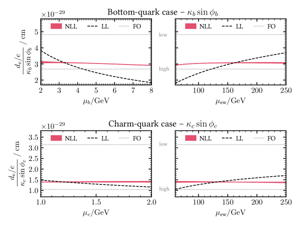
Figure 4: Residual scale dependence of the electric dipole moment induced by CP-odd bottom-quark couplings (upper two panels) and CP-odd charm-quark couplings (lower two panels). In the left two panels, the variation of the matching scale at the bottom and charm thresholds is shown, respectively, while the right two panels show the dependence on the electroweak matching scale. In all plots, the dashed lines show the scale variation of the LL result. The scale variation of the NLL results is indicated by the red bands. The boundaries of the red bands are obtained by the evaluating the NLL scale variation in two ways, as discussed in the main text. Finally, the two gray dotted lines show the fixed-order results that have been used in literature so far; they correspond to evaluating the quark masses in Eq. (3) at the electroweak scale (the line marked “high”) and at the heavy-quark threshold (the line marked “low”), and neglecting all other QCD corrections.

The corresponding results are further illustrated in the two upper and two lower plots of Figure 4 for the bottom- and charm-quark cases, respectively. The plots on the left show the scale dependence of $d_{e}/e$ on $\mu_{q_{h}}$ at LL (dashed, black line) and NLL (red band) accuracy. The plots on the right show the corresponding dependence on $\mu_{\text{ew}}$. For the LL result we use one-loop values for all masses and couplings, and both one- and two-loop values for the NLL result, as discussed above. The comparison of LL and NLL transparently shows how the NLL computation presented here drastically reduces the large uncertainties associated to QCD corrections.

Furthermore, the gray dotted lines in Figure 4 show the naive result of the fixed-order calculation, Eq. (3), that has been used so far in the literature. The two lines correspond to using different values for the heavy-quark mass $m_{q_{h}}$: the line marked “high” corresponds to using the value evaluated at the electroweak scale ($m_{q_{h}}(M_{h})$), while line marked “low” corresponds to using the mass evaluated at the low scale ($m_{q_{h}}(m_{q_{h}})$). The spread of these three lines illustrates the level of ambiguity in the fixed-order result. The NLL computation of the current work removes this ambiguity almost entirely.

The ACME collaboration has constrained the electron EDM to $|d_{e}|<1.1\times 10^{-29}$ at 90% confidence level [12]. To perform a rough combination of this experimental constraint with our derived theory uncertainties we interpret the measurement as a Gaussian centered at zero and the above bound as the correspodning 90% confidence level (CL) interval, i.e., including negative values for $d_{e}$. Adding the corresponding experimental “$1\sigma$” uncertainty in quadrature with the theory uncertainty we find based on an one-parameter $\chi^{2}$ function in terms of $\kappa_{q_{h}}\sin\phi_{q_{h}}$

$$\kappa_{b}|\sin\phi_{b}| <0.22\quad\text{[at 68.27\% CL]}\,, \kappa_{b}|\sin\phi_{b}|<0.36\quad\text{[at 90\% CL]}\,,$$ (41)

$$\kappa_{c}|\sin\phi_{c}| <0.48\quad\text{[at 68.27\% CL]}\,, \kappa_{c}|\sin\phi_{c}|<0.79\quad\text{[at 90\% CL]}\,.$$ (42)

5 Conclusions

The experimental bound on the electron EDM [12] translates into strong constraints on new CP-violating phases in various extensions of the SM (the SM contribution to the electron EDM is estimated to lie nine orders of magnitude below the current experimental sensitivity [21, 22]). CP-violating phases such as those in Eq. (1) appear in several well-motivated beyond standard model theories (see e.g. Refs. [9, 10]), and the electron EDM is capable of placing stringent bounds on these phases [4, 7, 8, 6].

However, implicit in these electron EDM bounds is a large ${\cal O}(1)$ QCD uncertainty that has so far been neglected, even though it leads to sizeable ambiguities in the resulting constraints. Fortunately, since the electron EDM is a leptonic observable, this ambiguity can be removed systematically by a perturbative calculation, without the need for additional non-perturbative information. In this work, we have calculated the contribution to the electron EDM of CP-odd Higgs couplings to the bottom and charm quarks in RG-improved perturbation theory, summing the leading and next-to-leading large logarithms proportional to the strong coupling constant. This calculation has reduced the residual ambiguity in the bound to the level of a few percent, as discussed in detail in Section 4. The perturbation series shows good convergence, as expected for a leptonic observable. If, in the future, a non-zero electron EDM were observed, the error could be further reduced by summing the next-to-next-to-leading QCD logarithms, as well as taking into account the QED evolution of the electric dipole moment below the heavy-quark thresholds.

Appendix A Unphysical Operators

For completeness, we list here the “unphysical” operators entering our calculation in intermediate steps. They are called “unphysical” because they vanish either via the equations of motion (e.o.m.) of the quark fields for onshell external states, or via algebraic relations that are valid in $d=4$, but not in $d\neq 4$.

A.1 E.o.m.-vanishing Operators

These operators have matrix-elements that vanish via the e.o.m. of the quark field. The following two gauge-invariant operators enter our computation at the two-loop level:

$$\begin{split}N_{1}^{e}&=\frac{m_{q_{h}}}{2e^{2}}\bar{e}\bigl{[}\stackrel{{\scriptstyle\leftarrow}}{{\not{D}}}\stackrel{{\scriptstyle\leftarrow}}{{\not{D}}}i\gamma_{5}+i\gamma_{5}\not{D}\not{D}\bigr{]}e\,,\\ N_{2}^{e}&=\frac{m_{q_{h}}}{2e^{2}}\bar{e}\bigl{[}\stackrel{{\scriptstyle\leftarrow}}{{\not{D}}}\stackrel{{\scriptstyle\leftarrow}}{{D^{\sigma}}}\gamma^{\mu}\gamma^{\nu}\gamma^{\rho}-\gamma^{\mu}\gamma^{\nu}\gamma^{\rho}D^{\sigma}\not{D}\bigr{]}e\,\,\epsilon_{\mu\nu\rho\sigma}\,.\end{split}$$ (43)

The covariant derivative acting on electron fields is defined as

$$D_{\mu}\equiv\partial_{\mu}+ieQ_{e}A_{\mu}\,,$$ (44)

with $Q_{e}=-1$ the electron electrical charge.

A.2 Evanescent Operators

Next we list the evanescent operators that enter our computation at one- and two-loop order. The leading-order ADM does not depend on their definition, but the next-to-leading-order ADM does. In the $q$–$q$–$A$ sector we need the operator

$$\begin{split}{E}_{\gamma}^{e}&=\frac{Q_{e}}{4}\frac{m_{q_{h}}}{e}\bar{e}\{\sigma^{\mu\nu},i\gamma_{5}\}e\,F_{\mu\nu}-Q_{3}^{e}\,.\end{split}$$ (45)

The evanescent operators required in the $e$–${q_{h}}$ sector read

$$\begin{split}{E}_{1}^{e{q_{h}}}&=\frac{1}{2}(\bar{e}\gamma_{[\mu}\gamma_{\nu]}e)\,({\bar{q}_{h}}\{\gamma^{[\mu}\gamma^{\nu]},i\gamma_{5}\}{q_{h}})+O_{2}^{e{q_{h}}}\,,\\ {E}_{1}^{{q_{h}}e}&=\frac{1}{2}({\bar{q}_{h}}\gamma_{[\mu}\gamma_{\nu]}{q_{h}})\,(\bar{e}\{\gamma^{[\mu}\gamma^{\nu]},i\gamma_{5}\}e)+O_{2}^{e{q_{h}}}\,,\\ {E}_{2}^{e{q_{h}}}&=\frac{}{}\big{[}(\bar{e}\gamma_{[\mu}\gamma_{\nu]}\gamma^{[\rho}\gamma^{\sigma]}e)\,({\bar{q}_{h}}\gamma^{[\mu}\gamma^{\nu]}\gamma^{[\tau}\gamma^{\upsilon]}{q_{h}})+(\bar{e}\gamma^{[\rho}\gamma^{\sigma]}\gamma_{[\mu}\gamma_{\nu]}e)\,({\bar{q}_{h}}\gamma^{[\tau}\gamma^{\upsilon]}\gamma^{[\mu}\gamma^{\nu]}{q_{h}})\big{]}\epsilon_{\rho\sigma\tau\upsilon}\\ &\quad-48(O_{1}^{e{q_{h}}}+O_{1}^{{q_{h}}e})+16O_{2}^{e{q_{h}}}\,,\\ {E}_{3}^{e{q_{h}}}&=\frac{1}{2}(\bar{e}\gamma_{[\mu}\gamma_{\nu}\gamma_{\rho}\gamma_{\sigma]}e)\,({\bar{q}_{h}}\{\gamma^{[\mu}\gamma^{\nu}\gamma^{\rho}\gamma^{\sigma]},i\gamma_{5}\}{q_{h}})-24O_{1}^{{q_{h}}e}\,,\\ {E}_{3}^{{q_{h}}e}&=\frac{1}{2}({\bar{q}_{h}}\gamma_{[\mu}\gamma_{\nu}\gamma_{\rho}\gamma_{\sigma]}{q_{h}})\,(\bar{e}\{\gamma^{[\mu}\gamma^{\nu}\gamma^{\rho}\gamma^{\sigma]},i\gamma_{5}\}e)-24O_{1}^{e{q_{h}}}\,,\\ {E}_{4}^{e{q_{h}}}&=\frac{1}{2}(\bar{e}\gamma_{[\mu}\gamma_{\nu}\gamma_{\rho}\gamma_{\sigma}\gamma_{\tau}\gamma_{\upsilon]}e)\,({\bar{q}_{h}}\{\gamma^{[\mu}\gamma^{\nu}\gamma^{\rho}\gamma^{\sigma}\gamma^{\tau}\gamma^{\upsilon]},i\gamma_{5}\}{q_{h}})\,,\\ {E}_{4}^{{q_{h}}e}&=\frac{1}{2}({\bar{q}_{h}}\gamma_{[\mu}\gamma_{\nu}\gamma_{\rho}\gamma_{\sigma}\gamma_{\tau}\gamma_{\upsilon]}{q_{h}})\,(\bar{e}\{\gamma^{[\mu}\gamma^{\nu}\gamma^{\rho}\gamma^{\sigma}\gamma^{\tau}\gamma^{\upsilon]},i\gamma_{5}\}e)\,,\\ {E}_{5}^{e{q_{h}}}&=\frac{1}{2}\big{[}(\bar{e}\gamma_{[\mu}\gamma_{\nu}\gamma_{\rho}\gamma_{\sigma]}\gamma^{[\tau}\gamma^{\upsilon]}e)\,({\bar{q}_{h}}\gamma^{[\mu}\gamma^{\nu}\gamma^{\rho}\gamma^{\sigma]}\gamma^{[\zeta}\gamma^{\xi]}{q_{h}})\\ &\qquad+(\bar{e}\gamma^{[\tau}\gamma^{\upsilon]}\gamma_{[\mu}\gamma_{\nu}\gamma_{\rho}\gamma_{\sigma]}e)\,({\bar{q}_{h}}\gamma^{[\zeta}\gamma^{\xi]}\gamma^{[\mu}\gamma^{\nu}\gamma^{\rho}\gamma^{\sigma]}{q_{h}})\big{]}\epsilon_{\tau\upsilon\zeta\xi}+48O_{2}^{e{q_{h}}}\,.\end{split}$$ (46)

The square brackets denote antisymmetrisation normalised as

$$\gamma_{[\mu_{1},...,\mu_{n}]}\equiv\frac{1}{n!}\sum_{\sigma}(-1)^{\sigma}\gamma_{\mu_{\sigma(1)}}\ldots\gamma_{\mu_{\sigma(n)}}\,.$$

A.3 Operators Related to the Infrared Rearrangement

The last class of unphysical operators arises because our use of infrared rearrangement breaks gauge invariance in intermediate steps of the calculation. At the renormalisable level this method generates two gauge non-invariant operators corresponding to a gluon-mass and a photon-mass term, i.e.

$$\mathscr{L}\supset\frac{1}{2}Z_{\text{IRA},g}Z_{G}\,m_{\text{IRA}}^{2}G_{\mu}^{a}G^{\mu,\,a}+\frac{1}{2}Z_{\text{IRA},\gamma}Z_{A}\,m_{\text{IRA}}^{2}A_{\mu}A^{\mu}\,.$$ (47)

The mass, $m_{\text{IRA}}$, is completely artificial and drops out of all physical results, and $Z_{\text{IRA},g}$, $Z_{\text{IRA},\gamma}$ are two additional renormalisation constants [23]. One-loop insertions of the dimension-five and dimension-six operators can induce further gauge-invariant, higher dimension operators that are relics of the infrared rearrangement. For our calculation, the only relevant one is

$$\begin{split}P^{e}&=m_{q_{h}}\frac{m_{\text{IRA}}^{2}}{e^{2}}\bar{e}i\gamma_{5}e\,.\end{split}$$ (48)

Appendix B Renormalization Constants

The following are the SM counterterms necessary for the calculation:

$$Z_{e}^{(0,1)} =\frac{2}{3\epsilon}\Big{[}N_{c}\big{(}n_{d}Q_{d}^{2}+n_{u}Q_{u}^{2}\big{)}+n_{\ell}Q_{e}^{2}\Big{]}\,,$$ (49)

$$Z_{e}^{(0,2)} =\frac{1}{\epsilon^{2}}\bigg{\{}\frac{2}{3}\Big{[}N_{c}\big{(}n_{d}Q_{d}^{2}+n_{u}Q_{u}^{2}\big{)}+n_{\ell}Q_{e}^{2}\Big{]}^{2}+\epsilon\Big{[}n_{\ell}Q_{e}^{4}+N_{c}\big{(}n_{d}Q_{b}^{4}+n_{u}Q_{c}^{4}\big{)}\Big{]}\bigg{\}}\,,$$ (50)

$$Z_{A}^{(0,1)} =-\frac{4}{3\epsilon}\Big{[}N_{c}\big{(}n_{d}Q_{d}^{2}+n_{u}Q_{u}^{2}\big{)}+n_{\ell}Q_{e}^{2}\Big{]}\,,$$ (51)

$$Z_{A}^{(1,1)} =\frac{1}{\epsilon}\big{(}1-N_{c}^{2}\big{)}\big{(}n_{d}Q_{d}^{2}+n_{u}Q_{u}^{2}\big{)}\,,$$ (52)

$$Z_{A}^{(0,2)} =-\frac{2}{\epsilon}\bigg{[}n_{\ell}Q_{e}^{4}+N_{c}\big{(}n_{d}Q_{d}^{4}+n_{u}Q_{u}^{4}\big{)}\bigg{]}\,,$$ (53)

$$Z_{m_{A}}^{(0,1)} =-\frac{8}{3\epsilon}\Big{[}N_{c}\big{(}n_{d}Q_{d}^{2}+n_{u}Q_{u}^{2}\big{)}+n_{\ell}Q_{e}^{2}\Big{]}\,,$$ (54)

$$Z_{{q_{h}}}^{(1,0)} =-\frac{1}{\epsilon}C_{F}\xi_{g}\,,$$ (55)

$$Z_{f}^{(0,1)} =-\frac{1}{\epsilon}Q_{f}^{2}\xi_{a}\,,$$ (56)

$$Z_{{q_{h}}}^{(1,1)} =\frac{1}{\epsilon^{2}}C_{F}Q_{q_{h}}^{2}\bigg{(}\xi_{g}\xi_{a}+\frac{3\epsilon}{2}\bigg{)}\,,$$ (57)

$$Z_{f}^{(0,2)} =\frac{1}{\epsilon^{2}}Q_{f}^{2}\bigg{\{}\frac{\xi_{a}^{2}}{2}Q_{f}^{2}+\epsilon\bigg{(}\frac{3}{4}Q_{f}^{2}+n_{\ell}Q_{e}^{2}+N_{c}\big{(}n_{d}Q_{d}^{2}+n_{u}Q_{u}^{2}\big{)}\bigg{)}\bigg{\}}\,,$$ (58)

$$Z_{m_{q_{h}}}^{(1,0)} =-\frac{3}{\epsilon}C_{F}\,,$$ (59)

$$Z_{m_{f}}^{(0,1)} =-\frac{3}{\epsilon}Q_{f}^{2}\,,$$ (60)

$$Z_{m_{q_{h}}}^{(1,1)} =\frac{9}{\epsilon^{2}}C_{F}Q_{q_{h}}^{2}\bigg{(}1-\frac{\epsilon}{6}\bigg{)}\,,$$ (61)

$$Z_{m_{q_{h}}}^{(2,0)} =-\frac{1}{\epsilon^{2}}\frac{C_{F}}{2N_{c}}\bigg{[}\frac{1}{2}\bigg{(}9-31N_{c}^{2}+4N_{c}(n_{u}+n_{d})\bigg{)}-\frac{\epsilon}{12}\bigg{(}9-203N_{c}^{2}+20N_{c}(n_{u}+n_{d})\bigg{)}\bigg{]}\,,$$ (62)

$$\begin{split}Z_{m_{f}}^{(0,2)}&=\frac{1}{\epsilon^{2}}Q_{f}^{2}\bigg{\{}\frac{9}{2}Q_{f}^{2}-2\big{(}n_{\ell}Q_{e}^{2}+N_{c}n_{d}Q_{d}^{2}+N_{c}n_{u}Q_{u}^{2}\big{)}\\ &\hskip 60.00009pt-\epsilon\bigg{(}\frac{3}{4}Q_{f}^{2}-\frac{5}{3}\big{(}n_{\ell}Q_{e}^{2}+N_{c}n_{d}Q_{d}^{2}+N_{c}n_{u}Q_{u}^{2}\big{)}\bigg{)}\bigg{\}}\,,\end{split}$$ (63)

where we have organised the contributions according to

$$Z_{i}=\sum_{m,n}\tilde{\alpha}_{s}^{m}\tilde{\alpha}_{e}^{n}Z_{i}^{(m,n)}\,.$$ (64)

and $f$ denotes either a charged-lepton or a quark field.

To obtain the two-loop anomalous dimension of the physical sector we need certain one-loop renormalisation constants involving unphysical operators. We collect them in this appendix. We write $Z_{x\to y}$ where the subscripts $x$ and $y$ symbolize sets of Wilson coefficients, for which we use the following notation and standard ordering:

$$\begin{split}P=\{&C_{1}^{e{q_{h}}},\,C_{1}^{{q_{h}}e},\,C_{2}^{e{q_{h}}},\,C_{3}^{e}\}\,,\\ E=\{&C_{E_{1}^{e{q_{h}}}},\,C_{E_{1}^{{q_{h}}e}},\,C_{E_{2}^{e{q_{h}}}},\,C_{E_{\gamma}^{e}}\}\,,\\ M=\{&C_{P^{e}}\}\,,\\ N=\{&C_{N_{1}^{e}},\,C_{N_{2}^{e}}\}\,.\end{split}$$ (65)

The first necessary input is the mixing of the physical operators into all the evanescent operators that are generated at one-loop. Using the same subscript notation as above, the renormalisation constants read

$$Z^{(0,1)}_{P\to E}=\begin{pmatrix}Q_{e}Q_{q_{h}}&0&0&0\\ 0&Q_{e}Q_{q_{h}}&0&0\\ 0&0&-\frac{1}{2}Q_{e}Q_{q_{h}}&0\\ 0&0&0&-4Q_{e}^{2}\end{pmatrix}\,,$$ (66)

and $Z^{(1,0)}_{P\to E}=0$. The remaining mixing of physical operators into evanescent operators is zero at one-loop. Furthermore, the finite part of the mixing of evanescent into physical operators is subtracted by finite counterterms [24]. They read

$$Z^{(0,1)}_{E\to P}=\begin{pmatrix}4Q_{e}Q_{q_{h}}&0&0&0\\ 0&4Q_{e}Q_{q_{h}}&0&0\\ 0&0&-8Q_{e}Q_{q_{h}}&0\\ 0&0&0&-\frac{2}{3}Q_{e}^{2}\end{pmatrix}\,.$$ (67)

The remaining finite mixing of evanescent into physical operators is zero at one-loop.

Furthermore, we need the mixing constants of the physical operators into the operators arising from infrared rearrangement; they are found to be

$$Z^{(0,1)}_{P\to M}=\begin{pmatrix}0\\ -12\\ 0\\ -12Q_{e}^{2}\end{pmatrix}\,.$$ (68)

All other mixing constants of physical into the IRA operators are zero.

Finally, we need the mixing constants of the physical operators into the e.o.m.-vanishing operators. They are uniquely fixed by the ${q_{h}}\to{q_{h}}$ Greens function. We find

$$Z^{(0,1)}_{P\to N}=\begin{pmatrix}0&0\\ 0&0\\ 0&0\\ -2Q_{e}^{2}&-\frac{1}{6}Q_{e}^{2}\end{pmatrix}\,.$$ (69)

The two-loop anomalous-dimension matrix is given in terms of the one- and two-loop renormalisation constants by

$$\gamma^{(0,2)} =4Z^{(0,2;1)}-2Z^{(0,1;1)}Z^{(0,1;0)}\,,$$ (70)

$$\gamma^{(1,1)} =4Z^{(1,1;1)}-2Z^{(0,1;1)}Z^{(1,0;0)}-2Z^{(1,0;1)}Z^{(0,1;0)}\,,$$ (71)

$$\gamma^{(2,0)} =4Z^{(2,0;1)}-2Z^{(1,0;1)}Z^{(1,0;0)}\,,$$ (72)

where we have further separated the renormalisation constants according to their poles, i.e.

$$Z_{i}^{(m,n)}=\sum_{r}\frac{1}{\epsilon^{r}}Z_{i}^{(m,n;r)}$$ (73)

The quadratic poles of the two-loop diagrams are fixed by the poles of the one-loop diagrams via

$$\begin{split}Z^{(0,2;2)}&=\frac{1}{2}Z^{(0,1;1)}Z^{(0,1;1)}-\frac{1}{2}\beta_{e}Z^{(0,1;1)}\,,\\ Z^{(1,1;2)}&=\frac{1}{2}Z^{(0,1;1)}Z^{(1,0;1)}+\frac{1}{2}Z^{(1,0;1)}Z^{(0,1;1)}\,,\\ Z^{(2,0;2)}&=\frac{1}{2}Z^{(1,0;1)}Z^{(1,0;1)}-\frac{1}{2}\beta_{0}Z^{(1,0;1)}\,,\end{split}$$ (74)

where $\beta_{0}=\frac{11}{3}N_{c}-\frac{2}{3}N_{\!f}$. As a check of our calculation, we computed these poles directly and verified that they satisfy Eq. (74).

References

[1]ATLAS collaboration, G. Aad et al., Observation of a new
particle in the search for the Standard Model Higgs boson with the ATLAS
detector at the LHC,
Phys. Lett. B716 (2012) 1–29,
[1207.7214].
[2]CMS collaboration, S. Chatrchyan et al., Observation of a New
Boson at a Mass of 125 GeV with the CMS Experiment at the LHC,
Phys. Lett. B716 (2012) 30–61,
[1207.7235].
[3]
E. Fuchs, M. Losada, Y. Nir and Y. Viernik, violation from ,
and dimension-6 Yukawa couplings - interplay of baryogenesis, EDM and
Higgs physics, JHEP05 (2020) 056,
[2003.00099].
[4]
J. Brod, U. Haisch and J. Zupan, Constraints on CP-violating Higgs
couplings to the third generation,
JHEP11
(2013) 180, [1310.1385].
[5]
D. Egana-Ugrinovic and S. Thomas, Higgs Boson Contributions to the
Electron Electric Dipole Moment,
1810.08631.
[6]
J. Brod and E. Stamou, Electric dipole moment constraints on
CP-violating heavy-quark Yukawas at next-to-leading order,
JHEP07
(2021) 080, [1810.12303].
[7]
H. Bahl, E. Fuchs, S. Heinemeyer, J. Katzy, M. Menen, K. Peters et al.,
Constraining the structure of
Higgs-fermion couplings with a global LHC fit, the electron EDM and
baryogenesis,
Eur. Phys. J. C82 (2022) 604,
[2202.11753].
[8]
J. Brod, J. M. Cornell, D. Skodras and E. Stamou, Global constraints on
Yukawa operators in the standard model effective theory,
JHEP08
(2022) 294, [2203.03736].
[19]
E. E. Jenkins, A. V. Manohar and P. Stoffer, Low-Energy Effective Field
Theory below the Electroweak Scale: Anomalous Dimensions,
JHEP01
(2018) 084, [1711.05270].
[20]Particle Data Group collaboration, P. A. Zyla et al., Review
of Particle Physics,
PTEP2020
(2020) 083C01.
[21]
M. E. Pospelov and I. B. Khriplovich, Electric dipole moment of the W
boson and the electron in the Kobayashi-Maskawa model, Sov. J. Nucl.
Phys.53 (1991) 638–640.