Modelling Slope Microclimates in the Mars Planetary Climate Model
Abstract
A large number of surface features (e.g., frost, gullies, slope streaks, recurring slope lineae) are observed on Martian slopes. Their activity is often associated with the specific microclimates on these slopes, which have been mostly studied with one-dimensional radiative balance models to date. We develop here a parameterization to simulate these microclimates in 3D Global Climate Models. We first demonstrate that any Martian slope can be thermally represented by a poleward or equatorward slope, i.e., the daily average, minimum, and maximum surface temperatures depend on the North-South component of the slope. Based on this observation, we implement here a subgrid-scale parameterization to represent slope microclimates (radiative fluxes, volatile condensation, ignoring slope winds for now) in the Mars Planetary Climate Model and validate it through comparisons with surface temperature measurements and frost detections on sloped terrains. With this new model, we show that slope microclimates do not have a significant impact on the seasonal CO2 and H2O cycles. Furthermore, short-scale slopes do not significantly impact the thermal state of the atmosphere. 91% of the active gullies are found where our model predicts CO2 frost, suggesting that their activity is related to processes involving CO2 ice. However, the low thicknesses ( tens of cm) predicted at mid-latitudes there rule out mechanisms involving large amounts ( meters) of ice. This model opens the way to new studies on surface-atmosphere interactions in present and past climates.
JGR Planets
Laboratoire de Météorologie Dynamique, Institut Pierre-Simon Laplace (LMD/IPSL), Sorbonne Université, Centre National de la Recherche Scientifique (CNRS), École Polytechnique, École Normale Supérieure (ENS), Paris, FranceInstitut d’Astrophysique Spatiale, Université Paris-Saclay, CNRS, Orsay, France
Lucas Langelucas.lange@lmd.ipsl.fr
We develop a sub-grid slope parameterization to simulate slope microclimates in the Mars Planetary Climate Model;
We test and validate this parameterization against observations; and reappraise frost thicknesses on Martian slopes;
This novel model opens the way to new studies on surface-atmosphere interactions for the present and past climates of Mars.
Plain Language Summary
Martian slopes present traces of present and past activities (e.g., dust avalanches, moraines created by past glaciers). Such activities are linked to the microclimate of these slopes: a slope oriented toward the pole will be more in the shadow and therefore colder than a slope oriented toward the equator. For now, mostly 1D models have been used to determine the microclimates present on these slopes, neglecting potential 3D atmospheric effects. Here we propose a parameterization allowing us to model such microclimates in 3D Global Climate Models. We have implemented and validated this parameterization in the Mars Planetary Climate Model by comparing our model with observations and measurements of these microclimates on the slopes. Our model shows that these slope microclimates do not significantly influence the global climate of Mars. We also provide a new CO2 ice thickness map which constrains the possible mechanisms that form gullies on Mars.
1 Introduction
Martian slopes are associated with a wide range of present-day surface processes [Diniega \BOthers. (\APACyear2021), Dundas \BOthers. (\APACyear2021)]. Gullies, surface features composed of an alcove, a channel, and a depositional apron similar to small terrestrial alluvial fans, are found on slopes at mid and high latitudes [Malin \BBA Edgett (\APACyear2000)]. At low to mid-latitudes, dark wedge-shaped features on high-albedo steep slopes are associated with downslope mass movements of the first micrometers of the surface, and are known as Slope Streaks [Sullivan \BOthers. (\APACyear2001)]. Dark features called Recurring Slope Lineae (RSL) are also found on steep slopes that have a low albedo [McEwen \BOthers. (\APACyear2011), McEwen \BOthers. (\APACyear2014)]. Other mass movements reported on Martian slopes include rockfalls and small displacements of high-latitude rocks [Dundas \BOthers. (\APACyear2019a)], polar avalanches [Russell \BOthers. (\APACyear2008)], and dune-slope activity [Diniega \BOthers. (\APACyear2019), Diniega \BOthers. (\APACyear2021)].
Although the origin of these features is still debated today, most of the mechanisms proposed to explain their activity are associated with the microclimates (surface/subsurface temperatures, condensation or sublimation of volatiles, near-surface winds) found on the slopes [<]e.g., ¿Diniega2021,Dundas2021. Because of the low thickness of the Martian atmosphere today, surface temperatures and near-surface environment are mostly controlled by radiative fluxes at the surface [Savijärvi \BBA Kauhanen (\APACyear2008)]. These fluxes are significantly modified for a slope compared to a flat surface. For instance, pole-facing slopes receive less solar insolation and are thus significantly colder than equator-facing slopes. Therefore, ice should preferentially accumulate on these slopes, as confirmed by current frost observations [Schorghofer \BBA Edgett (\APACyear2006), Carrozzo \BOthers. (\APACyear2009), Vincendon \BOthers. (\APACyear2010b), Vincendon (\APACyear2015), Dundas \BOthers. (\APACyear2019b), Lange \BOthers. (\APACyear2022)]. Consequently, sublimation-driven processes have been proposed to explain some pole-facing slope features that are consistent with the presence of CO2 or H2O ice [<]see¿[for a complete review]Diniega2021. Similarly, for slopes reaching the warmest temperatures, i.e., equator-facing slopes, thermally-stress-induced flows have been proposed to explain equator-facing slope features [<]e.g.¿[for RSL]Schmidt2017, Tesson2020.
Slopes also present traces of past climates of Mars. For instance, \citeAKreslavsky2011 reported moraines interpreted as remnants of CO2 glaciers on steep pole-facing slopes at high latitudes. These glaciers could correspond to periods of low obliquity when pole-facing slopes are cold traps that favor the condensation of the atmosphere [Kreslavsky \BBA Head (\APACyear2005)]. Conversely, at higher obliquity, around the summer solstice, surface and soil temperature of poleward-facing slopes could possibly reach the melting point of water, melting near-surface ice, possibly creating Martian debris flows features observed at mid-latitudes [Costard \BOthers. (\APACyear2002)].
The consequences of slope microclimates are not limited to the surface as they also influence the thermal environment of the Martian subsurface and its contents. The Gamma Ray Spectrometer [<]GRS,¿[]Boynton2004 onboard Mars Odyssey has revealed the presence of subsurface water ice covered by a dry layer of regolith above 55° latitude, and locally down to 45° [Boynton \BOthers. (\APACyear2002)], which was predicted/globally reproduced by numerical models [Leighton \BBA Murray (\APACyear1966), Mellon \BBA Jakosky (\APACyear1995), Mellon \BOthers. (\APACyear1997), Mellon \BOthers. (\APACyear2004), Schorghofer \BBA Aharonson (\APACyear2005)]. As pole-facing slopes are colder than surrounding flat surfaces, \citeASchorghofer2005 suggested that subsurface water ice (either pore-filling or excess ice) could be stable at equatorward latitudes beneath these pole-facing slopes. Local high-resolution subsurface ice mapping indeed showed that the depth of the ice table was correlated to topographic heterogeneity [Bandfield (\APACyear2007), Piqueux \BOthers. (\APACyear2019)]. \citeAAharonson2006 modeled the theoretical stability of subsurface water ice, considering the topographic heterogeneity at high resolution, by using a 1D thermal model that accounts for sloped terrains. They found that ice could be stable at latitude as close as ° compared to ° for former models that do not consider slopes and their particular thermal behavior. \citeAVincendon2010 also suggested that the absence of CO2 frost at low latitudes on steep south-facing slopes in the Southern hemisphere during winter could be explained by the presence of this subsurface water ice beneath these slopes. Such results have profound implications, especially as shallow water ice can be an exploitable resource for future crewed exploration [Morgan \BOthers. (\APACyear2021)].
Therefore slope microclimates are necessary to understand current surface and subsurface processes, as well as past climates of Mars. These processes are generally found on steep ( 20∘) slopes that have a typical length of kilometers/tens of kilometers [Kreslavsky \BBA Head (\APACyear1999)]. Such short-scale topographies and associated microclimates cannot be represented in a 3D Global Circulation Model (GCM) like the Mars Planetary Climate Model [<]Mars PCM, formerly known as the LMD-Mars GCM,¿Forget1999 which has a typical resolution of 300 km in longitude and 220 km in latitude at the equator. Mesoscale models with resolutions of tens of kilometers, either on a limited area or on the whole planetary sphere, cannot be used for long-term surface-atmosphere interactions (e.g., glacier evolution following obliquity variations over thousands of years) given prohibitive computational cost.
1D radiative equilibrium models are often used to study the environment on a slope [<]e.g., ¿Costard2002,Vincendon2010,Vincendon2010water. However, in most of these models, feedback on the large-scale properties of the meteorology is neglected while some surface processes are dependent on global circulations. For instance, surface water ice formation depends on the amount of water vapor and ice precipitation which need to be resolved by a GCM. For such studies, 1D models have been paired to outputs from 3D GCM as in \citeAVincendon2010water and \citeAWilliams2022.
In this context, the implementation of sub-grid scale slope microclimates in Mars GCMs is now required to better understand the present and past surface/subsurface processes that shape the Martian environment we know today. This problem is similar to the one faced by Earth climate modelers with the sub-grid scale diversity of topography, soil, or vegetation on Earth. They use several approaches to model the interaction between the land surface heterogeneity with the overlying atmospheric layer which are known as Land Surface Parameterization [Pitman (\APACyear2003), Flato \BOthers. (\APACyear2013), de Vrese \BOthers. (\APACyear2016)]. Common approaches used, like the ”mosaic” or ”mixture” strategies, divides the mesh into homogeneous discrete sub-divisions where microclimates evolve. Fluxes to the atmosphere are then computed by averaging all sub-grid scale values usually weighted by their respective cover fractions, by using more complex parameterizations [Giorgi \BBA Avissar (\APACyear1997)], or set to the values computed with the sub-division that has the largest cover fractions [Dickinson \BOthers. (\APACyear1986)].
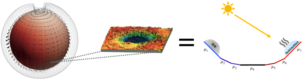
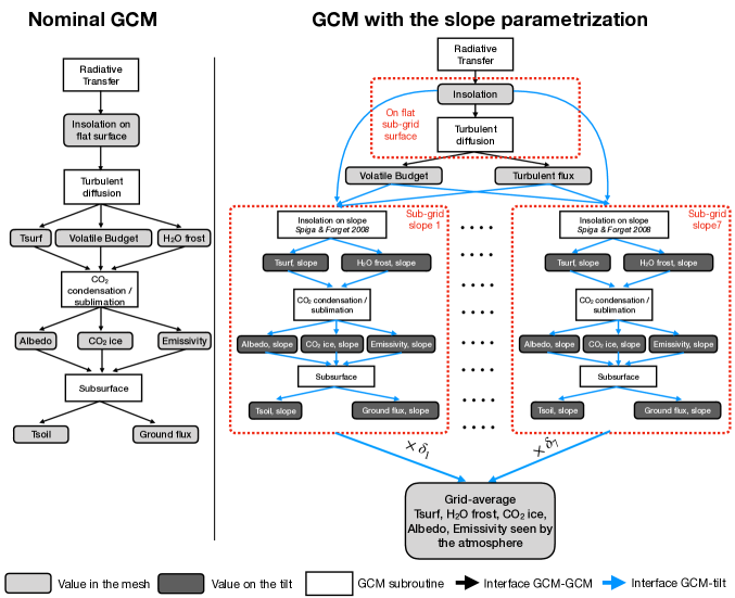
We propose here to develop for Mars a similar sub-grid scale parameterization that accounts for topographic heterogeneity. The principle is illustrated in Figure 1. For each GCM mesh, we decompose the cell as a distribution of sloped terrains (defined by characteristic slopes) and a flat terrain. On each sub-grid terrain, we let the microclimates evolve so that the slope-specific features (e.g., condensation of volatiles, formation of glaciers, migration of subsurface ice, etc.) can be simulated. The portion of the atmosphere above the ground within the cell sees an average of these surface microclimates, and all sub-grid terrains see the same ”shared atmosphere”.
In section 2, we present the construction of the sub-grid slope representation in the model. We then describe in section 3 the implementation of slope microclimates in the Mars PCM. An illustration of the capability of the model is given in section 4. The validation of these sub-grid scale microclimates is presented in section 5. Perspectives on the use of this new model are presented in section 6, and conclusions are drawn in section 7.
2 Representation of Slopes in the Mars PCM Meshes
The first step for the construction of our sub-grid slope parameterization is to determine a representative parameter of the surface inhomogeneity (i.e., the distribution of slopes within a mesh). We define the projected slope on the meridional direction as:
| (1) |
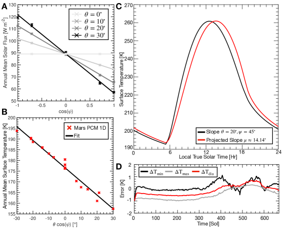
with the slope angle and the slope orientation. We demonstrate here that any given slope (, ) can be thermally, on average, represented by a slope with a slope angle of that is either North-facing if , or South-facing if . will be thus the representative parameter for our distribution. To do so, we used the one-dimensional energy balance code derived from the Mars PCM [Forget \BOthers. (\APACyear1999)] and described in \citeAVincendon2010, Vincendon2010water. In short, the 1D model computes the same physical processes as in the 3D model and runs with its local properties prescribed as inputs (slope angle, orientation, optical dept of the aerosols, etc.). The effects of large-scale meteorology or slope winds are not modeled in this 1D model. The 1D model uses the method described in \citeASpiga2008 to compute the radiative budget on slopes, taking into account scattering by aerosols and the thermal emission from adjacent flat surfaces. We ran the model for several slope angles and azimuths on several locations on Mars, using a nominal dust opacity profile derived by averaging the available observations of dust from Martian Year (MY) 24, 25, 26, 28, 29, 30, and 31 outside the global dust storm period [Montabone \BOthers. (\APACyear2015)] which is referred to as clim dust scenario in the rest of the manuscript. Figure 2a illustrates satisfying linear correlations (R 0.95 in all cases) found between the parameter and the annual mean solar flux defined as the sum of the solar flux at infrared and visible wavelengths calculated by the model. Equivalent conclusions can be drawn using other simulations made at different latitudes. Similarly, a linear relationship (R 0.97) can be found between the projected slope and the surface temperature (Figure 2b). This linear relationship illustrates the fact that for any given slope (, ), the radiative energy budget can be, on average, represented by a slope with a slope angle of that is either North-facing if , or South-facing if .
We test this assumption by computing several surface temperatures for a given slope () and the corresponding North/South-facing slope with a slope angle at different latitudes. An illustration is given in Figure 2c for a diurnal cycle and confirms that the North/South slope emulator has the same thermal behavior as the initial slope (). The difference between the two surface temperatures is caused by the difference in the slope’s azimuths, which create a phase shift that evolves during the sol and the position of the sun in the sky. Apart from this phase shift, the minimum, maximum, and daily-mean surface temperatures are consistent (relative error lower than 1%) throughout the year (Figure 2d). The instantaneous error, created by the time lag between the two temperatures, barely exceeds 5% of the instantaneous surface temperature and is neglected. Therefore, this confirms that any sub-grid scale slopes in the Mars PCM can be either represented by pole-facing slopes or equator-facing slopes when one wishes to study the behavior of ice or any process sensitive to the diurnal or seasonal variation of surface and subsurface temperatures. Yet, our model might be limited when studying processes on East/West slopes due to the time lag between the North/South slope and the initial slope (). One other approach used by \citeAWilliams2008 is to consider an equivalent latitude and an adjusted longitude computed from , to correct this time shift. However, this approach was more difficult to implement in the current Mars PCM without increasing significantly the computation time as it requires recomputing the radiative transfer at each equivalent latitude and an adjusted longitude. Thus, this approach has not been adopted for our parameterization. Furthermore, in this 1D experiment, we do not consider the possible heterogeneity of albedo, thermal inertia, or the possible influence of slope winds. These effects are discussed later in section 3.4.3, 3.4.5.
We then need to find how to discretize the north-south projected slopes to decompose our mesh into a limited subset of representative sub-grid scale slopes (Figure 1). To do so, we studied the distribution of computed with the Mars Orbiter Laser Altimeter [<]MOLA,¿Smith2001 data that have been widely used to study the Martian topography and slope distribution [<]e.g.,¿Smith2001, Kreslavsky2000, Aharonson2003. We used the 1/64° dataset corresponding to a resolution of nearly 1 km at the equator which corresponds to the typical length of key geomorphological features observed at the surface of Mars [<]e.g.,¿Head2003, Kreslavsky2011, Hobbs2013. Note that the MOLA resolution used depends on the user’s desired resolution for the sub-grid surface, and that lower or higher resolutions can be used. The MOLA data used are in a simple cylindrical format, and we have not corrected them for Mars’ non-sphericity, assuming it has only a minor effect. Given the two-dimensional topographical field where and are the distance in meters respectively in the longitude and the latitude direction, and the altitude in meters at coordinates , the slope angle and the slope orientation can be computed with Eq. 2 and 3 [Spiga \BBA Forget (\APACyear2008)]:
| (2) |
| (3) |
where , . Derivatives are calculated using centered differences with neighboring pixels. The projected slope is then computed. The distribution of is presented in Figure 3. A complete analysis of the Martian slope distribution is out of the scope of this paper, but the results obtained here (predominance of flat surfaces on Mars, the limited number of steep slopes, etc.) are consistent with dedicated studies using the same dataset and similar resolution [Kreslavsky \BBA Head (\APACyear1999), Kreslavsky \BBA Head (\APACyear2000)]. The distribution of slopes obtained is sensitive to the resolution of the MOLA dataset used. As noted in \citeAAharonson2006, a high-resolution topographic dataset promotes steep slopes at the expanse of flat surfaces. Yet, at a resolution of hundreds of meters, their results (see their Figure 6) are consistent with ours, i.e., flat surfaces predominate over slopes. At very low scales (resolution 10 m), where steep slopes are significant contributors, the Mars PCM physics and parameterizations are not adapted and would be in the domain of the Large-Eddy Simulations.
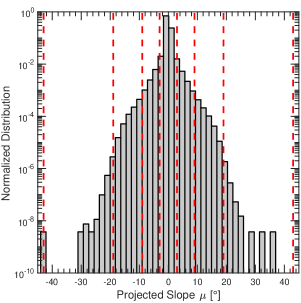
We then defined seven slope classes (delimited by the red lines in Figure 3 and defined in Table 1) that are representative of the projected slope distribution. Each mesh of the Mars PCM is divided into 7 sub-grid scale slopes that are either north-facing or south-facing, defined by a characteristic presented in Table 1. We assume that this partition with seven sub-grid surfaces (1 for the flat one, and 6 for the slopes) allows us to represent the distribution of slopes within the meshes. We could have added more classes for the decomposition but this would have increased the computation time too much without much scientific gain. Also, we cannot decrease the number of classes too much because we would lose a realistic representation of the distribution within the mesh (i.e., we would have a flat terrain and only extreme slopes). The characteristic proposed in Table 1 are computed as the means of the endpoints of the slope classes (except for the class 1 and 7 where it is set to 30°), rather than an average of weighted by the distribution within the class. The typical slope used to represent a class is exaggerated (by 1° for classes 3-5; 3° for classes 2-6 for instance, 5° for classes 1-7). This choice was motivated by future studies which required modeling steep (25°) slopes (see for instance sections 5, 6).
| Class | Definition | Characteristic | ||
| 1 | -43° -19° | ° | ||
| 2 | -19° -9° | ° | ||
| 3 | -9° -3° | ° | ||
| 4 | -3° 3° | ° | ||
| 5 | 3° 9° | ° | ||
| 6 | 9° 19° | ° | ||
| 7 | 19° 43° | ° |
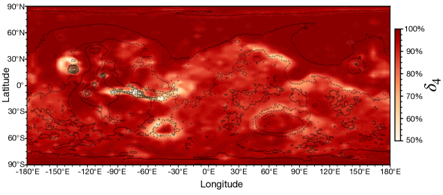
For each mesh of the Mars PCM and each characteristic slope , we can compute the percentage of the area of the cell occupied by slopes that are in a class (this percentage is noted hereinafter and called cover fraction). In this computation, the variable size of the MOLA pixels within a Mars PCM grid because of the latitude is considered. Here, and for the rest of the manuscript (if not explicitly stated), the resolution of the Mars PCM grid was 5.625° in longitude, and 3.75° in latitude (i.e., 330 km 220 km, a standard resolution for the PCM for which the high resolution is 60 km 60 km, i.e., 1° 1°). Results for class 4, i.e., for quasi-flat terrains, are presented in Figure 4. The distribution of the flat sub-grid surface obtained (Figure 4) is consistent with what is presented in the literature [<]e.g., Figure 6 of ¿Aharonson2006. Most of the sloped terrains are logically found in Valles Marineris, Hellas Planitia, Elysium Planitia, and the North-South dichotomy. It should be noted that at this spatial resolution, the predominant sub-grid surface (i.e., the one with the largest cover fraction) is the flat terrain. To avoid numerical artifacts, we assume that the whole mesh is flat when the area occupied by the slopes is smaller than 0.001% of the total mesh area.
Another important quantity for our parameterization is the shape of the distribution of the sub-grid slopes within a mesh. Are the sub-grid slopes uniformly distributed or on the contrary, a sub-slope is largely predominant? We calculated for each mesh the kurtosis of the real (and not discretized as in Table 1) distribution of the sub-grid slopes computed from the MOLA dataset. The kurtosis is a mathematical parameter that measures the tailedness of the distribution. To simplify, a high kurtosis suggests that the distribution is highly concentrated around its mean, while a low kurtosis suggests a rather uniform distribution. All the calculated kurtosis are high, even for cells where the flat sub-grid surface is less dominant. The distribution of the sub-grid slopes is very narrow and centered on the flat sub-slope. We also tested these properties with a high-resolution GCM grid (1°1°). In that case, for some meshes, the predominant sub-grid surface is a sloped one (e.g., in Valles Marineris), and the distribution is still tight and centered on this slope. Only 1% of the GCM grid does not have a clear peak in the sub-grid slope distribution. The consequences of the properties of the distribution are discussed in the next section.
3 Sub-Grid Scale Microclimates Modelling
We propose the following parameterization to simulate slope microclimates, inspired by the ”mosaic” and ”mixture” strategies in Earth models [de Vrese \BOthers. (\APACyear2016)]. On each binned slope, we calculate the radiative energy budget at the mesh center. Section 2 showed us that, at the given spatial resolution, the flat sub-grid surface strongly dominates. One can view the Martian topography within a mesh as a predominantly flat terrain with some sporadic slopes (where a significant amount of volatiles can condense, however). Turbulent exchanges mostly take place with the flat terrain, the slopes making only negligible contributions to the mixing. We thus assume that turbulent exchanges are solved with the predominant sub-grid surface. We compute and let evolve independently on each sub-grid slope the surface and subsurface temperatures, the volatile budget, and ground properties. We assume that these sub-grid slopes are independent and share the same atmosphere. The atmosphere only sees an averaged value of these surface fields, weighted by their cover fraction. The implementation of this strategy is detailed in Figure 5.
3.1 Energy budget on a slope
The evolution of the surface temperature is computed based on the energy budget at the surface:
| (4) |
where the left member of the equation is the energy of the surface layer, with is the density of the ground (kg m-3), cs is the ”surface layer” heat capacity per unit area (J m kg-1 K-1) and is related to the thickness of the first soil layer, the sub-grid slope temperature (K), (unitless) the albedo of the surface, the radiative flux at visible wavelengths (W m-2), (unitless) is the surface emissivity (assumed to be equal to the absorptivity), the radiative flux at infrared wavelengths (W m-2), the soil heat flux due to heat conduction process (W m-2), the sensible heat flux, the latent heat flux due to the condensation/sublimation of a volatile with a latent heat (J kg-1) and the radiative cooling of the surface with = 5.67 W m-2 K-4 the Stefan-Boltzmann constant. We describe below the computation of each term.
The resolution of Eq. 4 is made using an implicit scheme and the soil heat conduction is solved using a finite volume approach to the problem. Surface temperature is technically linked to atmospheric and ground processes which are coupled. Following the strategy of \citeAHourdin1995, the resolution is made as follows: the internal energy of the surface layer, and thus the surface temperature, is updated at time using Eq. 4. Temperatures of the subsurface layers are then updated by solving the thermal conduction. Once these temperatures are computed, the soil heat flux is computed and given as an input of Eq. 4 for the next time step.
3.1.1 Radiative Fluxes
The computation of radiative fluxes accounts for CO2 gas infrared absorption/emission [Hourdin (\APACyear1992), Forget \BOthers. (\APACyear1999), Dufresne \BOthers. (\APACyear2005)], dust absorption, emission, diffusion in the visible and infrared [Forget (\APACyear1998), Forget \BOthers. (\APACyear1999), Madeleine \BOthers. (\APACyear2011)], and the radiative effect of water ice clouds [Madeleine \BOthers. (\APACyear2012)]. Dust opacity is set based on the maps from \citeAMONTABONE2015 and we used in the following the clim dust scenario.
The total irradiance computed with the current method must be adapted when considering a sloped terrain. , which accounts for direct incoming flux from the sun, scattered flux by dust in the atmosphere, and the reflected flux from the neighboring terrains is computed with the parameterization from \citeASpiga2008. For thermal infrared radiation, we assume that the atmospheric thermal radiation is isotropic and we note (W m-2) the atmospheric incident thermal infrared flux on a horizontal surface computed by the PCM. Here, for a given sub-grid slope, we assume that the rest of the mesh is flat to be consistent with \citeASpiga2008. The sky-view factor (unitless), which quantifies the proportion of the sky in the half hemisphere seen by the slope that is not obstructed by the surrounding terrain, is defined as in \citeASpiga2008:
| (5) |
where refer to the absolute value of the projected slope .
Based on geometrical considerations, the thermal infrared radiation for a sloped surface can be written as
| (6) |
where (unitless) is the emissivity sub-grid flat terrain, (K) its temperature. Here, we neglect the possible influence of the atmosphere (both in terms of absorption and diffusion) on the emission from the flat surface.
3.1.2 Sensible and Latent Heat Flux
The sensible heat flux describes the energy exchange between the atmosphere and surface due to molecular conduction and turbulence. Such flux can be written as [Forget \BOthers. (\APACyear1999)]:
| (7) |
where (m s-1) is the wind velocity obtained by combining the large-scale (synoptic) wind near the surface with a gustiness wind induced by buoyancy [Colaïtis \BOthers. (\APACyear2013)], (J kg-1 K-1) is the air specific heat capacity at constant pressure, (K) the temperature of the atmosphere in the 1st vertical layer of the GCM (about 4 m above the surface) and (unitless) is a heat transfer coefficient given by [Colaïtis \BOthers. (\APACyear2013)]:
| (8) |
where is a function of the Richardson number , (unitless) is the von Karma constant set to 0.4; (m) is the aerodynamic roughness coefficient extracted from \citeAHebrard2012, (m) the thermal roughness length. The computations of and are detailed in \citeAColaitis2013. and are computed when considering the predominant sub-grid terrain.
For each sub-grid surface, water ice deposition and sublimation are computed following \citeANavarro2014:
| (9) |
where (kg m-2) is the mass of H2O frost, normalized by unit area, is the mass mixing ratio of water vapor in the first layer, is the saturation mass mixing ratio at the surface temperature [<]see Eq. (1) of ¿Pal2019. The latent heat flux is then computed by multiplying by with the latent heat of sublimation of water at , computed from a 2nd-order polynomial fit of \citeAFEISTEL200736’s data.
In the model, convection near the surface promotes water sublimation through the gustiness wind induced by buoyancy [Colaïtis \BOthers. (\APACyear2013)] and the stability function . However, this convection is assumed to be dry, induced by the thermal contrast between the surface and the atmosphere. We, therefore, neglect convection induced by the molecular gradient of the air linked to the presence of water near the surface [<]e.g.,¿Ingersoll1970. We assume that the vapor pressure of water at the surface is too low to affect the molecular weight of the air and that turbulent mixing at the surface should limit the impact of this free convection [Ivanov \BBA Muhleman (\APACyear2000)]. However, this assumption can be questioned in the case of frost with warm temperatures close to the melting point [Schorghofer (\APACyear2020)]. However, the model predicts water ice with a temperature 220 K, which legitimizes our approximation. However, further work is needed to include these effects in future studies, particularly in the case of ice stability at high obliquity, where melting is expected [Costard \BOthers. (\APACyear2002)]. This requires a reparameterization of surface fluxes and a wet convection model that are beyond the scope of the paper. Nevertheless, the effect of the water latent heat term is generally neglected on Mars as it is often reduced to 1-2 W m-2 today [<]e.g.,¿Richardson2002, Martinez2014; although it can become significant at higher obliquity [Naar \BOthers. (\APACyear2021)].
CO2 deposition and sublimation computations and the latent heat associated are made following \citeAForget1998snow. For ground condensation, as CO2 is abundant in the atmosphere if the surface temperature on a sub-grid slope predicted by radiative and conductive balance (i.e., Eq. 4 solved without any condensation/sublimation of CO2 ) falls below the condensation temperature at surface pressure (given by the Clapeyron’s law using the partial pressure of CO2 , \citeAJammes1992), the amount of CO2 condensing (kg m is:
| (10) |
where (J kg-1) is the latent heat of CO2 . This expression is almost similar to the one of \citeAForget1998snow except we add the term which corresponds to the extra heat brought by the atmosphere when cooled to the condensation temperature just above the surface. Even if the temperature is cooled by Eq. 7 and radiative processes, in the case of a pole-facing slope, the lower atmosphere lying just above the surface can be significantly warmer than the surface so this term can be significant. Typically, can be 15 K higher than on frosted pole-facing slopes. As such, the extra heat brought by the atmosphere when cooled can reach nearly 2% of the latent heat. In the case of atmospheric precipitation (CO2 snow, but also other volatile deposition), we assume a uniform deposition on the whole mesh. Once is known, it is injected in Eq. 4 which will give, after integration, to be if there is CO2 ice on the surface.
3.1.3 Conduction in the soil and subsurface water ice
The computation of the ground flux is based on the 1D layer soil model originally described by \citeAHourdin1993 but rewritten for a physical vertical grid (in meters). The current Mars PCM solves the conduction in the soil from 2 m to 25 m, corresponding respectively to the minimum diurnal skin depth for a thermal inertia of 30 J m-2 K-1 s-1/2 and the maximum annual skin depth for a thermal inertia of 2000 J m-2 K-1 s-1/2, range of thermal inertia observed on Mars [Mellon \BOthers. (\APACyear2000)]. Optical properties (albedo, emissivity) of the surface are set as described in Table 2 based on the Thermal Emission Spectrometer (TES) measurements [Christensen \BOthers. (\APACyear2001)]. We assume that all the frost-free sub-grid surfaces have the same optical properties. Compared to the former version of \citeAHourdin1993, the current Mars PCM enables variations in the thermal properties (volumetric specific heat, thermal conductivity) with depth so that the effect of subsurface water ice can be included in the GCM. The high and mid-latitude subsurface ice reservoirs have a significant impact on the Martian climate. Because of their high thermal inertia, they store large amounts of heat during summer and restore them during winter. It thus significantly affects the CO2 cycle through the ice deposition/sublimation [Haberle \BOthers. (\APACyear2008)] and can prevent/reduce the condensation of CO2 on pole-facing slopes [<]see ¿ [for a complete discussion on the effect of subsurface ice on slope energy budget]Vincendon2010,KhullerGullies. In the current model that does not consider sub-grid slopes, maps of the ice table are created using measurements by the Mars Odyssey Neutron Spectrometer (as part of GRS) of the abundance of hydrogen near the surface [Feldman \BOthers. (\APACyear2002), Feldman \BOthers. (\APACyear2004)] and an inversion model of the effective depth of the water ice table [Diez \BOthers. (\APACyear2008)].
Few observational constraints on the ice table under a slope exist [<]e.g.,¿Khuller2021ice because of 1) the resolution of the instruments (more than 500 km for the spectrometers [Saunders \BOthers. (\APACyear2004)]); 2) the paucity of high-resolution observations allowing a fine determination of the ice table on the slopes [Bandfield (\APACyear2007), Vincendon \BOthers. (\APACyear2010a), Piqueux \BOthers. (\APACyear2019)]. To take into account the thermal effect of the ice table on the slopes, we must model their distribution. To do so, we used the theory proposed by \citeALeighton1966, Mellon2004, Schorghofer2005, Aharonson2006: a subsurface ice (either massive ice or pore-filling) at a depth z is stable if:
| (11) |
where overbars indicate time averages over a complete Martian year, (Pa) is the water vapor pressure at the surface, (Pa) is the saturation water vapor pressure over water ice which is a function of the temperature [Murphy \BBA Koop (\APACyear2005)]. \citeAMellon1993, Schorghofer2005, Aharonson2006 used radiative equilibrium with fixed humidity, based on the values retrieved by the TES [Smith (\APACyear2002)] and do not simulate the complete water cycle. Recent sensitivity studies have shown that subsurface water ice stability is sensitive to atmospheric conditions [Song \BOthers. (\APACyear2023)] as well as the presence of surface water frost [Hagedorn \BOthers. (\APACyear2007), McKay (\APACyear2009), Williams \BOthers. (\APACyear2015)]. Here, with the Mars PCM, we can compute more accurately the water cycle which has been validated through TES data [Navarro \BOthers. (\APACyear2014), Naar \BOthers. (\APACyear2021)] and thus the vapor density at the surface considering all of these effects. We set to the near-surface vapor pressure given by the GCM if the surface is not ice-covered, if it is ice-covered. When ice is stable at depth , we set the thermal inertia of this layer and those below to 1,600 J m-2 K-1 s-1/2, a mid-value between completely pore-filled ice [<]thermal inertia of 1200 W m-2 K-1; Eq. (26) of ¿Siegler2012 and massive pure ice [<]thermal inertia of 2050 W m-2 K-1 at 180 K;¿Hobbs1974.
As water ice enhances conduction and thus the propagation of thermal waves to depth, it attenuates shallow depth temperature fluctuations, which decrease the mean vapor density and promotes the stability of subsurface water ice. Hence, the algorithm is iterated until an equilibrium is reached for the ice table depth. With this approach, we simulate for the first time the distribution of the ice table underneath slopes but also flat surfaces with a complete GCM for the atmosphere and the (sub)surface. The results will be presented in a dedicated paper [Lange \BOthers. (\APACyearsubmitted)].
Map Inputs Input Source Thinnest Spatial Resolution Data Uncertainty Resolution used Topography MOLA [Smith \BOthers. (\APACyear1999)] 500 m 1–3 m [Neumann \BOthers. (\APACyear2001)] 1 km Thermal Inertia TES [Putzig \BOthers. (\APACyear2005)] 3 km 8% of the thermal inertia value [Putzig \BOthers. (\APACyear2005)] PCM resolution Albedo – bare ground TES [Putzig \BOthers. (\APACyear2005)] 3 km 0.5% of the albedo value [Putzig \BOthers. (\APACyear2005)] PCM resolution Surface Roughness Derived from TES rock abundance [Hébrard \BOthers. (\APACyear2012)] 7 km Between 10-2 to 10-4 m [Hébrard \BOthers. (\APACyear2012)] PCM resolution Constant inputs Input Range of value observed Value used in this study Albedo - H2O ice 0.25-0.6, depending on dust contamination and grain size (Langevin 2005) 0.33 Albedo - CO2 ice 0.25-0.65 [Titus \BOthers. (\APACyear2001), Langevin \BOthers. (\APACyear2007)] 0.65 Emissivity – bare ground 0.75-1 [Bandfield \BBA Smith (\APACyear2003)] 0.95 Emissivity – H2O ice 0.95-1 [Vincendon \BOthers. (\APACyear2010b)] 1 Emissivity – CO2 ice 0.8-1 [Titus \BOthers. (\APACyear2001), Piqueux \BOthers. (\APACyear2016)] Computed after \citeAForget1998snow
3.2 Interaction between sub-grid surfaces and the atmosphere
Once the microclimates have been computed and sub-grid surface properties updated, we need to communicate this information to the atmosphere by updating the mesh values. Following Earth model conventions [de Vrese \BOthers. (\APACyear2016)], grid parameters are determined by averaging all sub-grid parameter values weighted by their respective cover fractions. In practice, we assume that the grid box albedo and emissivity can be computed with :
| (12) |
where refers to the grid parameter, the sub-grid parameter of slope , the cover fraction.
In the model, condensed volatiles at the surface (i.e., seasonal frost or perennial ice) are represented with surface mass density (kg m-2). However, the area of the sloped mesh grid is not the same if it is sloped or flat, assuming a similar latitude/longitude boundary for the cell. Hence, to ensure mass conservation, condensed volatiles at the surface are computed with :
| (13) |
where is defined in Table 1.
For surface temperature, we assume that we can average the Stefan–Boltzmann function:
| (14) |
where (unitless) is the grid emissivity, (K) the grid surface temperature, and quantities with subscript refer to the same quantities but for the sub-grid slope.
3.3 Post-Processing and Interpolation
The proposed model allows, for each grid point, to determine the surface fields for the seven types of slopes modeled here (Figure 1, Table 1). The question is now: for any point on the Martian surface, knowing the characteristics of the terrain (slope and azimuth), can we determine the values of the surface quantities (e.g., CO2 frost, H2O frost, surface temperature) using the GCM outputs that are discretized in space and slopes?
Let us consider a point (noted ) of the surface of Mars, placed on a surface of slope angle and azimuth . We compute and find the index of the two GCM sub-grid slopes such that:
| (15) |
The point is surrounded by four GCM meshes. We can interpolate the values obtained at the GCM points for the sub-grid slope and at point . This is performed by using a bilinear interpolation in space. After that, the value for slope at is obtained with linear interpolation between the fields obtained after the bilinear interpolation for and . If or , an extrapolation is computed. Thus, we have virtually access to any surface field for any kind of sloped surface on Mars using this complete climate model. We acknowledge that 1) we assume linear interpolation on processes that are not necessarily linear (although we interpolate neighboring points); 2) we neglect the time-shift (generally lower than 1-2 hours) for slopes oriented East-West (Figure 2c).
3.4 Discussions on the Modeling Assumptions
3.4.1 East-West component of the slope
We have demonstrated in section 2 that our parameterization is suitable to represent the diurnal (minimum, maximum, and daily mean) and seasonal variations of the (sub)surface temperatures of any slopes through its projected slope . However, the parameterization is not adapted to reproduce the instantaneous (sub)surface temperature for a slope with an East-West component. As shown in Figure 2c, d, the time shift created by the azimuth of the slope is not reproduced when simulating the thermal behavior of the slope with the parameter . This will impact the comparison with surface temperature measurements (section 5.1: the impact can be as high as 10-15 K) (Figure 2c).
3.4.2 Effect of surrounding topography
It is assumed for the computation of the reflected flux that for a given sub-grid slope, the rest of the mesh is flat. We acknowledge here that this assumption is simplifying but considering non-flat surrounding terrains would generate a much more sophisticated form factor calculation [<]e.g.,¿Dozier1990, as well as a radiative coupling problem between all sub-grid surfaces [<]e.g., section 2. of¿Schorghofer2022. Furthermore, the model neglects shadowing created by surrounding slopes. Hence, cold traps found in alcoves for instance [Schorghofer (\APACyear2020)] are not well represented.
3.4.3 Sub-grid surface thermophysical properties
We assume that the thermophysical properties (albedo, emissivity, thermal inertia, see Table 2) of the coarse-resolution main grid apply to the sub-grid surfaces (if they are frost-free). However, surface heterogeneities have been observed at km scale [<]e.g.,¿Ahern2021, which can lead to significant differences in the surface temperatures. For instance, an error of 100 J m-2 K-1 s-1/2 on the thermal inertia can lead an error of 10 K on the surface temperature [<]Figure 1 of ¿Putzig2007; an error of 0.1 on the albedo or on the emissivity would lead to an error of less than 5 K [<]Figure 1 of ¿Putzig2007,Bandfield2008. Nevertheless, our assumption seems reasonable as no clear constraints exist for the slope surface properties: some exhibit dust/sand [<]e.g.,¿Tebolt2020 while others expose bedrock/high thermal inertia material [<]e.g.,¿Edwards2009.
3.4.4 Turbulent exchanges and common atmosphere between the sub-grid surfaces
We assumed in the parameterization that the turbulent exchanges are done with the predominant sub-grid surface and that all sub-grid surfaces share the same atmosphere. We acknowledge here that this scientific can be discussed. For instance, Earth climate models have shown that turbulent mixing processes can be significantly different when sub-grid variability is considered [Mahrt (\APACyear2000), Molod \BOthers. (\APACyear2003), de Vrese \BOthers. (\APACyear2016)]. However, on Mars unlike on Earth, surface-atmosphere thermal exchanges are strongly dominated by radiative fluxes (computed for each slope) rather than turbulent sensible heat flux [Read \BOthers. (\APACyear2017)].
The assumption that sub-grid surfaces share a common atmosphere column can also lead to inaccuracies, particularly in near-surface thermal environments. The near-surface atmosphere energy budget is primarily controlled by the radiative process associated with the slope over the first 500 m (i.e., reflected irradiance and atmospheric absorption). Above 500 m, the increasing thermal gradient leads to the dominance of convection for the next several kilometers [Read \BOthers. (\APACyear2017)]. As a result, the first few hundred meters of the atmosphere may be colder over a poleward-facing slope than over a flat area. It should be noted that even if convection is not dominant, it would also alter the near-surface environment, and help to homogenize the atmosphere [Colaïtis \BOthers. (\APACyear2013)]. However, building a parameterization for this convective activity for km slope, i.e., in the ’grey zone’ [<]or ’Terra Incognitae’¿Wyngaard2004 for resolved/parameterized convection would require a dedicated study using Large Eddy Simulations and is out of the scope of this paper.
The infrared emission by the atmosphere comes mainly from altitudes between 2 and 10 km [<]Figure 2 of ¿Dufresne2005. The atmosphere at these altitudes is not influenced by small slopes [<]less than 1 km in height difference, as observed on craters for instance, e.g.,¿Vincendon2010,Vincendon2010water because it is mixed by winds at altitudes that do not see this small relief. For these terrains, the approximation of a shared atmosphere for the calculation of the infrared flux is therefore valid. For more significant slopes (important differences in level or length of several tens of km, e.g., canyon), this hypothesis is more questionable in addition to the non-consideration of the slope winds which might play a major role. Furthermore, our approach assumes that the winds will effectively mix these air masses such that one can adopt a common atmospheric column for all sub-grid surfaces in the analysis. Indeed, the observed Martian slopes in our study tend to be a few kilometers wide and are separated by distances on the order of tens of kilometers. The near-surface winds have speeds of several meters per second which can mix the atmosphere between slope regions over periods of nearly tens of minutes. With our physical time-step of 15 minutes, we assume that this time is enough to mix the air masses and have a common atmospheric column between the sub-grid slopes.
3.4.5 Effect of slope winds on the sensible and latent heat
Because of the low density and heat capacity of the Martian atmosphere, the sensible and latent heat terms generally lead to negligible contributions compared to the radiative fluxes in the Martian surface energy budget [Savijärvi \BBA Määttänen (\APACyear2010), Martínez \BOthers. (\APACyear2014)]. However, \citeASpiga2011 have demonstrated that during the night, katabatic winds can locally reinforce the sensible heat flux which becomes comparable to the thermal infrared cooling of the surface. Anabatic slope winds could also explain colder than expected surface temperatures during the afternoon [Spiga \BOthers. (\APACyear2011)].
Slope winds have also an effect on the sublimation of H2O as it is controlled by the wind velocity (Eq. 9). As slope wind speeds can be 10 times higher than those for a flat surface, they can have great importance when modelling H2O ice stability. Experiments using the 1D model showed that high slope winds could reduce the ice stability by tens of sols [Vincendon \BOthers. (\APACyear2010b)].
Subgrid-scale parameterization of slope winds deserves a dedicated study and is left as a future work on how its impact on slope microclimates can be represented in Global Climate Models.
3.4.6 Interpolation sub-grid surfaces and grix box average
Grid-box average (section 3.2) or post-processing 3.3) are done using (bi)linear interpolation or linear average, weighted by the cover fraction. However, such methods are applied to processes that might be non-linear. These interpolations/communications between sub-grid heterogeneity and GCM grid box have been studied and reviewed in the Earth climate community [<]e.g.,¿Giorgi1997 and future improvements of our parameterization should focus on this point.
4 An illustration in the Olympus Mons Region
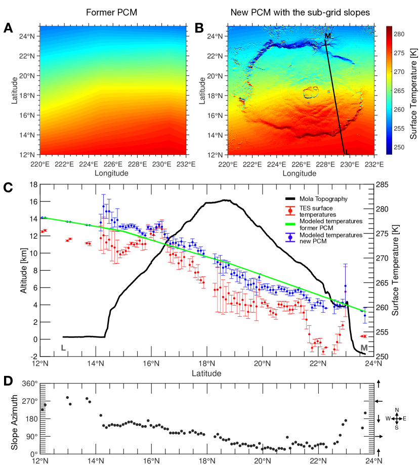
Here we illustrate the improvements achieved with this sub-grid slope parameterization by giving an example in the region of Olympus Mons (12°-25°N, 220-235°E). Figure 6a illustrates the surface temperatures predicted by the PCM without the parameterization. In this version, surfaces modeled by the PCM are only flat, so no temperature variation related to topography can be detected. Figure 6b illustrates the surface temperatures predicted by the PCM with the sub-grid parameterization in this same region, after the post-processing described in section 3.3. With this version, the obtained ”thermal image” and the surface temperature distribution of the area are more realistic: surface temperatures vary with the topography and the slopes. The reliefs of Olympus Mons appear naturally because of the topographic gradients that create surface temperature differences. We recover expected observations: the flanks of Olympus Mons oriented toward the equator are warmer than those oriented towards the North. The same conclusions for the caldera of the volcanoes can be drawn. Similar observations are drawn when repeating this experiment in different regions (e.g., Valles Marineris, Tharsis, etc.). This example is used for the validation in the next section.
5 Validations of the Implementation
5.1 Validation of the Surface Temperature
We compare here the surface temperatures predicted by our model on slopes with observations on warm (daytime), intermediate (dawn/sunset), and cold (night/shadow) surfaces. To do so, we used surface temperatures measured by TES and the Thermal Emission Imaging System [<]THEMIS,¿Christensen2004 infrared imager. The TES instrument includes a spectrometer in the 6-50 m band and co-aligned visible (0.3 - 2.7 m) and thermal (5.5-100 m) bolometers providing measurements with a 3-8 km resolution in a 380 km footprint. [Christensen \BOthers. (\APACyear2001)]. THEMIS includes a thermal bolometer in the 7-15 m band. and provides surface temperatures measurements with a resolution of m within a footprint of km. In this study, we use TES kinetic surface temperatures derived from spectral measurements because of their low sensibility to atmospheric effects [Bandfield \BBA Feldman (\APACyear2008)]. Furthermore, the emissivity used for TES retrievals is equal to the one of the PCM. THEMIS measures spectral radiance emitted by the surface and converts it to brightness temperature assuming a surface emissivity of one and without applying atmospheric correction [Christensen \BOthers. (\APACyear2003)]. Therefore, to mitigate these effects, we only considered surface temperatures acquired by THEMIS after 6 p.m. and before 8 p.m., or between 6 a.m. and 8 p.m. At these local times, simulations with the PCM indicate that the temperature contrast between the atmosphere and the surface should be low, so atmospheric correction, which is not done during THEMIS post-processing, should be low. Furthermore, we assume that at these times, the surface has cooled enough so that the effects of albedo variability during the day on temperatures have disappeared. We also assume that just after sunset, the effect of thermal inertia heterogeneity on slopes is not yet significant enough to introduce a bias during the comparison. For this last point, observations at 5 p.m. would have been preferable but the effect of slope azimuth on surface temperatures would still have been marked at these hours. Since these temperatures are calculated assuming an emissivity of 1 and the PCM assumes an emissivity of 0.95 we corrected these temperatures by a factor . Lastly, as THEMIS has a thin resolution, we have degraded the images to a resolution of 1 km, a resolution similar to the parameterization used in this section (MOLA file with a resolution of 1 km at the equator to generate the sub-grid statistics).
5.1.1 Daytime surface temperatures
For the daytime comparison, we looked at the Olympus Moons region, which has steep slopes and a surface with homogeneous properties. We present a comparison at Ls = 270° (Northern autumn) at 2 p.m in Figure 6c. TES measurements presented here have been made during Martian Year 26 on the transect AB (Figure 6b). For each measurement, we retrieved the slope angle and azimuth associated and computed the predicted surface temperatures using the method presented in section 3.2. We then binned the measurements and simulated temperatures on 0.1° latitude segments. As expected, the distribution of the surface temperatures with the parameterization is better (mean error of -4.2 K at 1- ) compared to the former PCM (mean error of -4.5 K at 1- ). The model performs less well (error of 5 K) when the slope has a strong east-west component (e.g., latitude s 16-19°N, Fig. 6d). This is due to the choice of representing the slope by its meridional component, which therefore does not lead to a satisfactory simulation of the instantaneous temperature for this type of slope. Surface temperatures are overestimated by the PCM, especially on the flank of the volcano where the steepest slopes are found. This might be caused by the katabatic slope winds (not represented in the model) which should cool down the atmosphere and decrease the surface temperatures [Spiga \BOthers. (\APACyear2011)]. Other surface temperature transects investigated show similar results in this region, as well as in Valles Marineis.
5.1.2 Sunset surface temperatures
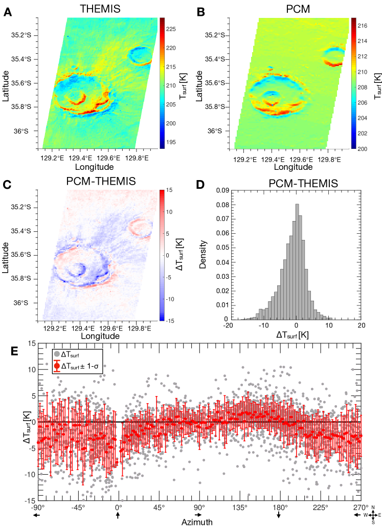
We then looked at temperatures acquired at sunset, which are intermediate during the warm temperatures of the day and cold ones at dawn. An example of validation is presented in Figure 7. Here, we looked at the area at Gasa crater (35.7°S, 129.4°E) during Southern spring. In this region of interest (ROI, defined by the boundaries given in Figure 7a), the majority of the surfaces is flat, and the steep terrains are confined to the craters where significant slopes can be found ( = 85% here). THEMIS measured surface temperatures that are on average 210 K, mostly on flat surfaces (Figure 7a) with extreme temperatures found on East-South and West-Equatorward facing slopes (between 200 K and 227 K respectively). The former PCM, without the sub-grid slope parameterization, i.e., which computes surface temperature only for flat terrains, gives a mean surface of 209 K, in good agreement with THEMIS observations but was not able to reproduce the cold and hot temperatures found on the slopes. The new parameterization helps to reproduce a realistic field where thermal contrasts created by the topography are apparent (Figure 7b). The difference between the PCM and THEMIS surface temperatures (Figure 7c) reveals two interesting features. First, some differences exist between the PCM and the observations on flat surfaces (e.g., 35.2-35.5°S, 129.4-129.6°E). These small differences are due to sub-kilometer variability in the thermal inertia that is not caught by the PCM. Second, the PCM seems to underestimate the surface temperatures on equatorward-facing slopes compared to THEMIS, whereas it overestimates it for pole-facing slopes (Figure S1a). However, Figures 7c, e show that the most significant differences are found on East-West slopes (Figure 7c, e), where the PCM can be 4 K ( K at 1- ) colder for a North-East-facing slope, or ( K at 1- ) K warmer for a South-West facing. On the contrary, for North-South facing slopes, the differences are limited to less than 1-2 K ( K at 1- ). Again, this is due to the slope parameterization, which does not model the slope’s azimuth effects (section 3.4.1). Thermal inertia effects also contribute to the difference between the observed and simulated temperatures as the slopes presented here present a higher thermal inertia ( 1000 J m-2 K-1) than the one used in the PCM (210 J m-2 K-1 s1/2). Finally, this underestimation of maximum and minimum temperatures on slopes may be linked to: 1) the common atmosphere between each sub-slope: North-facing slopes have a colder near-surface atmosphere than in reality, which could lead to an underestimation of the flow. This underestimation would be limited to 1 W m-2, given that the radiation comes mainly from an altitude of 2-10 km [Dufresne \BOthers. (\APACyear2005)], where atmospheric temperatures are homogeneous; 2) An overestimation of a scattering component for steep slopes, as the parameterization of \citeASpiga2008 is indeed less efficient for such slopes. Nevertheless, when comparing the temperatures simulated and observed on steep (slope angle 9°) slopes (Figure 7d), we observed that the modeled temperatures have an error of -1.3 K K at 1- . Other comparisons lead to other locations give similar results.
5.1.3 Cold surface temperatures at dawn
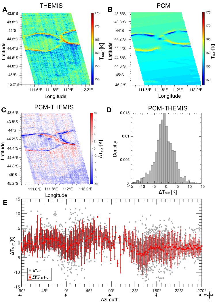
We checked here our surface temperatures with observations acquired at dawn when the surface temperatures are the coldest. An illustration is given in Figure 8. The image was acquired at 7.41 a.m. during Southern Winter. Shadowed pole-facing slopes have a surface temperature that is within 5 K of the CO2 frost point (150 K for the typical pressure at this location), suggesting the presence of CO2 ice [Khuller \BOthers. (\APACyear2021), Lange \BOthers. (\APACyear2022)]. As the emissivity of CO2 ice varies with crystal size [Piqueux \BOthers. (\APACyear2016), and references therein], we did not apply the correction for these areas. The observation of CO2 frost on pole-facing slopes at such latitudes is consistent with observations from \citeAVincendon2010,KhullerGullies,Lange2022a. The same observations as those described previously are found here: sub-grid differences between the model and the observations that are created by sub-grid differences of thermal inertia, and the influence of the slope azimuth. When comparing the slope surface temperatures (Figure 8d, Fig S1b), we found that the model is colder than the observations (-1.1 5 K at 1- ). The difference varies with the slope’s orientation (Figure 8e), with again, pole-facing slopes being warmer and equatorward facing slopes being colder by 2-3 K ( 4 K).
5.1.4 Generalization and conclusion
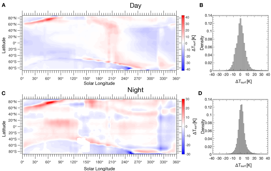
We extend the study presented above to other regions of Mars. Similar conclusions to those presented above can be drawn. The average surface temperatures predicted by the PCM and what is observed by THEMIS are consistent, even though small offsets can appear. We have quantified this difference over the year and planet by comparing the zonally average surface temperature measured by TES over MY 26 [Smith (\APACyear2004)] to the values computed by the PCM. As TES values in \citeASmith2004 are binned by 3° 3° of latitudes and longitudes, and 5° of Ls, we have compared these values to the surface grid-box averaged values given by the PCM. The comparison for daytime (2 p.m.) and nighttime (2 a.m.) is presented in Figure 9.
The PCM generally slightly overestimates surface temperature by K during summer and underestimates by K during winter. On average, during the year, the PCM marginally overestimates the surface temperature by +0.5 6 K at 1- during the day, and by 1.5 6 K at 1- during the night. This difference was also present in the former PCM without the parameterization and does not come from our work. This might be related to the vertical representation of dust/water in the PCM as the temperature differences (outside of polar regions) are mostly found during periods of high opacity (e.g., Ls= 180°-210°, Figure 9a)). Such conclusions can be extended to slope temperatures. Previous sections have shown that these temperatures were very sensitive to the slope azimuth and its thermal inertia. Nevertheless, we found a good agreement between our model and the observations. The agreement is better for short-scale topography (e.g., small crater, Figures 7, 8) than significant topographic gradients (e.g., Valles Marineis, volcanoes, Figure 6) where slope winds can significantly impact the slope energy budget [Spiga \BOthers. (\APACyear2011)].
These tests validate the overall good agreement between our model and the slope temperatures. However, we acknowledge that we cannot fully validate the surface temperatures on all slopes with our parameterization because of the difficulty of correcting the phase shift induced by the East-West components of the slopes and the under-mesh heterogeneity for the surface properties which can lead to differences up to 10-15 K between the model and the observations as presented by Figures 6, 7, 8 which are representatives of the error made. Again, the purpose of our parameterization is to represent the average thermal behavior of the slopes (diurnal average temperatures, minimum and maximum temperatures) and cannot fully simulate the instantaneous behavior. This is why we validate in the next section our parameterization with the observation of seasonal frost, which can theoretically be correctly represented by the parameterization.
5.2 Modelling the Distribution of Seasonal Frost on Slopes
5.2.1 Temporal Distribution
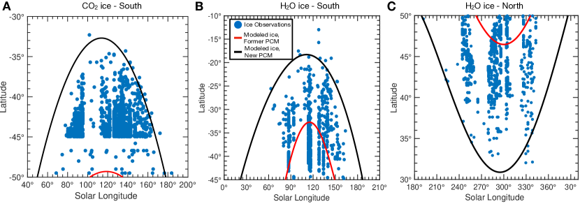
We now compare the distribution of seasonal CO2 and H2O frosts on slopes with the predictions of the PCM. For this validation, we used the frost detections made by OMEGA (Observatoire pour la Minéralogie, l’Eau, les Glaces et l’Activité) and CRISM (Compact Reconnaissance Imaging Spectrometer for Mars) instruments as reported in \citeAVincendon2010,Vincendon2010water,Vincendon2015. These detections were made using near-infrared spectroscopy in the afternoon, and correspond to seasonal frost. Hence, diurnal frost forming during the night and sublimating during the early morning is not considered [Piqueux \BOthers. (\APACyear2016), Khuller \BOthers. (\APACyear2021), Lange \BOthers. (\APACyear2022)]. These observations are compared with the prediction of CO2 and H2O ice stability on a 30° pole-facing slope retrieved from the PCM simulations at the same local time, i.e., 2 p.m. Following \citeAVincendon2010, we assume that CO2 ice is stable and should be detected by CRISM/OMEGA at a given latitude if the of CO2 ice thickness predicted on the slope by the PCM exceeds m at Ls 120°, 1000 m before. The threshold used is higher for Ls 120° because of the low signal-to-noise ratio on the slope at this time of the Martian year. Imposing a lower threshold (e.g., 100 m) would lead to an earlier condensation by 5 degrees of Ls, and an equatorward extent of the distribution by 3° of latitude. For H2O ice, the thickness threshold is set to m [Vincendon \BOthers. (\APACyear2010b)]. The comparison is presented in Figure 10.
CO2 ice:
The PCM with the sub-grid slope parameterization predicts CO2 ice on 30° pole-facing slopes in the southern hemisphere up to 33°S while the former PCM could predict CO2 ice on flat surfaces as low °S. This new latitudinal extent is consistent with observations by CRISM and OMEGA which detected CO2 frost on south-facing slopes up to 32.3°S. We observed an overall very good agreement between our modelling predictions and actual CO2 detections.
The timing of condensation/sublimation is consistent with the observations, even though both start slightly too early (by 5-10°). \citeAVincendon2010 showed that the beginning of condensation is sensitive to the amount of dust in the atmosphere, the presence of ice in the subsurface, and the thermal inertia of the surface. Dust is set to the observations of \citeAMONTABONE2015 and can not be tuned to match the observations. The subsurface ice is predicted to be stable at a depth of m in the 35°-45°S-band (see section 3.1.3). At such depth, subsurface ice has almost no impact on the surface energy budget and CO2 ice distribution. Hence, the difference between our model and the CO2 ice observations suggests shallower ice that is not predicted by our ice stability model. One can also delay the beginning of the modeled CO2 condensation/sublimation by modifying slope surface properties. However, no clear constraints exist for these properties as some slopes exhibit low thermal inertia [Tebolt \BOthers. (\APACyear2020)], favoring the condensation of CO2 ; while some slopes reveal high-thermal inertia bedrock exposures [Edwards \BOthers. (\APACyear2009)] which delay the formation of CO2 frost. Finally, one should note that the difference in the timing of condensation is observed at Ls °, a time where fewer ice observations are available because of the low illumination in this period, lowering the signal-to-noise ratio, and potentially preventing some detections.
Here, our model matches well the observations without relying on subsurface ice as in \citeAVincendon2010. This may be due to the fact that our model considers the surrounding plains that warm the atmosphere, increasing the downwelling infrared flux and therefore the surface temperature. Such effects, which were not considered in [Vincendon \BOthers. (\APACyear2010a)], and their consequences are discussed in section 6.1 and will be more detailed in a companion paper [Lange \BOthers. (\APACyearsubmitted)].
H2O ice:
Similar conclusions can be drawn when looking at the predicted latitude-season stability diagram for H2O ice (Figure 10b. and c.) The latitudinal extent of H2O ice is well predicted (as low as 30°N and 18 °S vs. 48 °N and 33 °S for the former PCM), even if few deposits at low latitudes (e.g., the one close in Valles Marineris at latitude 12.7°S) are not predicted by our model. In our experiment, the broadband albedo of H2O ice is set to 0.33 as it enables a good fit of the seasonal water cycle in the PCM [Naar \BOthers. (\APACyear2021)]. Similarly to \citeAVincendon2010water, increasing the albedo leads to a delay by a few degrees of Ls in the sublimation of the deposits. The sublimation of these deposits is also sensitive to wind speed. Here, this speed might be underestimated because the model does not compute slope winds although this should not significantly impact our results [Vincendon \BOthers. (\APACyear2010b)]. The beginning of the condensation of H2O is also too early by 10° of Ls in the PCM compared to the observations, as for the CO2 ice. This might be due to an observational bias in the autumn high latitude water ice detections at these longitudes [Vincendon \BOthers. (\APACyear2010b)], and a bias of our model that might underestimate surface temperature at this season as reported previously. One should note that our results are quite similar to those obtained by \citeAVincendon2010water.
5.2.2 Spatial Distribution
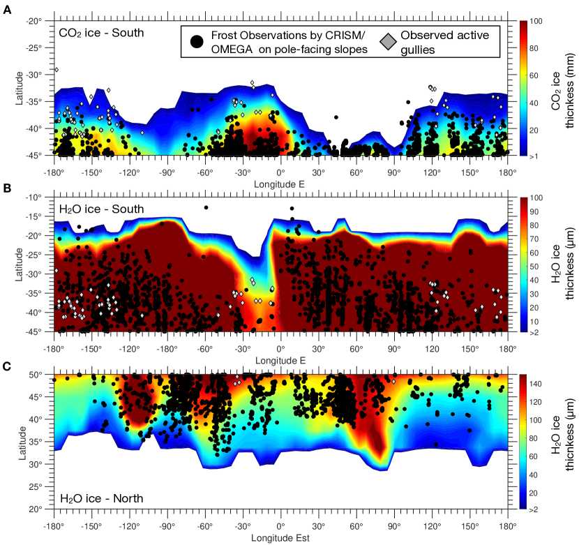
We also validate our parameterization by comparing the spatial distribution of CO2 and H2O ice observed by CRISM/OMEGA with our model. Results are presented in Figure 11.
CO2 ice:
Similarly to \citeAVincendon2010, the latitudinal stability limit of CO2 ice on any slope (Figure 11a) varies with longitude, with a mean value of 33°. Below 33°, ice might be present but as thin deposits ( 100 m). CO2 ice between -120°- -60°E, i.e., Thaumasia regions, is predicted to be thinner compared to the rest of the longitudes because of the higher altitude in this place, and thus the lower temperature of CO2 condensation. Our statistics of sub-grid slopes also suggest that the lack of CO2 ice detections in this region might be linked to the few numbers of steep ( 30°) south-facing slopes in this area. Interestingly, we found that CO2 ice detections by CRISM/OMEGA correlate with thick CO2 ice predicted by the model, while \citeAVincendon2010 proposed that deposits of few hundred of microns should be detected. The overall agreement validates our model for CO2 deposits. Few points are not predicted (e.g., the detection at 32.3°S on the East of Hellas) but this might be linked to favorable local conditions or the resolution of our model (3.75° of latitude) which might be not precise enough to differentiate what happens within a very few degrees of latitude. One can note that the model does not predict ice in Hellas Basin whereas it has been observed on flat surfaces (Piqueux et al., 2015) and on the rare steep slopes present at this place (Vincendon et al. 2010a). This is because of a systematic error in the Mars PCM (also present without the parameterization of slopes) which is under investigation.
H2O ice:
Similar conclusions can be drawn when looking at the spatial distribution of water ice. In the South (Figure 11b), our model reproduces well the observations, with notably the dry area in the band -40°E - 0°E where thinner frost (or no frost) is expected, as confirmed by the low amount of detections in this area. This is a consequence of the western jet on the eastern side of the Tharsis bulge [Joshi \BOthers. (\APACyear1994), Joshi \BOthers. (\APACyear1995)] leading to a dryer atmosphere (less water vapor available to form HO frost) [Vincendon \BOthers. (\APACyear2010b)]. Again, the model predicts ice in the Thaumasia region which is not observed. The same explanations as those mentioned above for CO2 ice, similar to those given by \citeAVincendon2010water, can be given. Locally, the latitudinal stability is higher than what is predicted by \citeAVincendon2010water (e.g., -180°E - -150°E) and explains some low latitude ice detections. In the North, the model predicts well the areas where numerous detections are made, as well as dry areas (e.g., -180°E - -150°E) where fewer ice deposits are observed by CRISM/OMEGA.
6 Discussions and Perspectives
6.1 Relationship between the atmosphere and the slope microclimates
One may first wonder if the slope microclimates impact the global climate. It is assumed here that the atmosphere sees an average of the sub-grid fields, weighted by the cover fraction. In section 2, we showed that the predominant sub-surface is the flat one (non-flat sub-grid surfaces represent 5% of the overall area). A significant impact of the slope microclimates on the global climate was thus not expected. We checked this assumption by comparing PCM runs with and without this parameterization and found little differences. For instance, the relative difference of the total mass of CO2 ice that condenses during the year between simulation with and without the sub-grid slope parameterization is lower than 1%. Similar conclusions can be drawn for the amount of H2O ice, and the total amount of H2O in the atmosphere. This is because 1) steep slopes, which accumulate a larger amount of frost compared to flat surfaces, are sparse and of limited length [<]tens or hundreds of meters,¿Aharonson2006; 2) regionally, some areas with a lot of pole-facing slopes have an excess of ice when considering the parameterization, but this is balanced by areas with a lot of equatorward-facing slopes, which have lower amounts of ice.
To date, slope microclimates have mostly been explored with 1D models [<]e.g.,¿Aharonson2006,Vincendon2010 which neglect contribution from the large-scale atmosphere dynamic. Therefore, one may wonder about the impact of the global climate on slope microclimates. In the 1D PCM used in \citeAVincendon2010,Vincendon2010water, the atmosphere is in radiative equilibrium with the surface studied. For a pole-facing slope, the atmosphere above it is therefore cold. However, in our 3D model, we assume that the atmosphere is horizontally mixed at the scale of the slopes. The atmosphere sees an average of sloped and flat sub-grid surfaces. As steep sloped terrains represent actually a small percentage of the overall surface of Mars (see section 2), the atmosphere is mostly in equilibrium with the warmer flat sub-grid surface. Hence, in the 3D model, the air close to cold sloped surfaces is warmer than in the 1D model as it is warmed by the nearby warm plains. This legitimates the computation of other models [<]e.g.,¿Mellon2001,Aharonson2006,Schorghofer2006,Kieffer2013 which used the same atmospheric infrared radiation for flat surfaces and steep slopes. Also, during winter, warm air is brought above pole-facing slopes because of the subsidence from the Hadley cell at mid and subtropical latitudes, which leads to adiabatic heating of the atmosphere [Barnes \BOthers. (\APACyear2017)]. This warmer atmosphere increases the downwelling infrared flux and thus modifies the amount CO2 /H2O ice condensing on the surface. Note that this effect is mostly pronounced for areas with a strong thermal contrast between the slopes and the flat surfaces and is thus most significant for low-latitude slopes ( 45∘N). These two effects increase the slope energy budget by nearly 10 W m-2, with significant consequences for CO2 frost extent. A more accurate description and demonstration of these two effects and their consequences are discussed in a companion paper [Lange \BOthers. (\APACyearsubmitted)]. As discussed in sections 3.4.4 and 3.4.5, this assumption of a ”shared” atmosphere, mostly in equilibrium with the flat surfaces, might lead to a small overestimation of the downwelling infrared flux, as cold air can, for instance, be confined within a crater by katabatic slope winds during the night and early morning. This might explain why our model has a too early starting of the CO2 sublimation (Figure 10) compared to the observations, but our choice is reasonable to study small/medium topographic relief.
6.2 Reappraisal of the frost thicknesses and consequences for the activity of gullies
Estimating the thickness of seasonal frosts (H2O or CO2 ice) on slopes is an important constraint for models of gully activity associated with sublimation processes [Dundas \BOthers. (\APACyear2019b), Diniega \BOthers. (\APACyear2021)]. No measurements of these thicknesses have been made and they have only been estimated by 1D models to date. Such studies only estimate frost thickness for specific locations and not at a global scale [<]e.g., ¿Schorghofer2006,Vincendon2015,KhullerGullies. We provide in Figure 11 a complete mapping (220 330 km of resolution) of the expected maximum CO2 frost thickness across the year for 30° pole-facing slopes. Compared to most of the 1D models used in the literature, our model with the sub-grid slope parameterization takes into account the seasonal CO2 cycle that has been validated against observations, CO2 depletion at polar latitudes, and the effects of large-scale meteorology. The seasonal frost thickness logically decreases with latitude, from a few mm at 33°S (3° of latitude due to the model resolution) to a few tens of cm at 45°S. Equatorward of 33°S, the model predicts 0.1 millimeters frost forming during the night which disappears during the morning, as observed by \citeAKhullerGullies,Lange2022a. Our model predicts larger ice thicknesses for mid and high latitudes (tens of cm). Interestingly, we find that in the southern hemisphere, the amount of CO2 that condenses on a 30° pole-facing slope has a similar frost thickness to the amount that condenses on flat terrain at about ten degrees of latitude lower. For example, at 41°S, 5 cm of frost can form on a 30° pole-facing slope, which is the same amount as that observed at the edge of the seasonal cap at 48°S (Litvak 2004). This is not observed in the Northern Hemisphere because of the shorter winter for the current eccentricity of Mars. However, as mentioned previously, this phenomenon will not impact the global mass of CO2 that will condense during the winter because these very steep slopes are rare on Mars and of limited length [<]tens or hundreds of meters,¿Aharonson2006. The longitudinal variations of frost thickness reflect the variations in surface properties (albedo, thermal inertia), and altitude. For water, we find a distribution similar to that of \citeAVincendon2010water who used a 1D model coupled with precipitation maps obtained in 3D. The frost thicknesses obtained are larger in our model by ten’s/hundreds of micrometers because the water cycle of the 3D model has been improved [Naar \BOthers. (\APACyear2021)] and is now wetter compared to the version used by \citeAVincendon2010water.
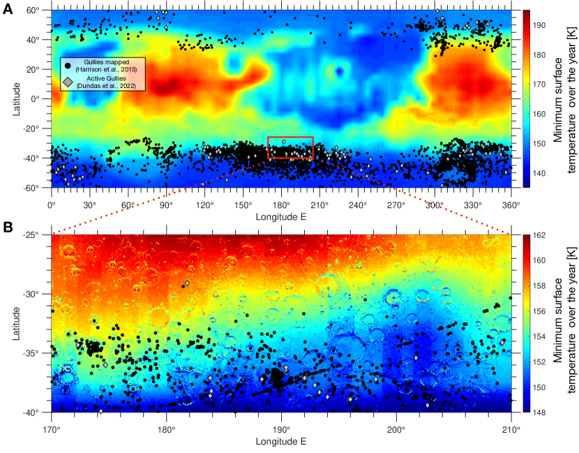
These new frost maps, compared to the map of active gullies, give us important information for modeling gully activity on Mars. Indeed, near-infrared observations suggest that active gullies are highly correlated to the presence of CO2 frost [Vincendon (\APACyear2015)]. By constructing high-resolution surface temperature maps with the method described in section 3.3 (Figure 10), we can see that the location of most of the active gullies indeed coincides with slopes where CO2 condensation occurs. More specifically, we found that the model predicts frost on 30° slopes on 91% of the active gully sites and 86% of all gully sites in the South. In the North, this percentage is reduced to 56% for active sites and only 9% for all gullies. Our derived values are upper limits as the amount of ice is predicted for steep (30°) pole-facing slopes for which the frost is most stable. Using a lower slope angle would hence reduce the statistics presented there. Nevertheless, our numbers are consistent with the same statistics derived in \citeAKhullerGullies. Hence, both observations and modeling suggest that the activity of gullies is mostly related to processes involving CO2 ice. However, the model does not predict a significant amount of CO2 ice (a few cm thick, Figure 11a), thus disfavoring models that require a significant amount of ice [<]e.g., ¿[although this model is for linear gullies which are mostly found above 45° latitude, where thicker ice is expected]Diniega2013, and promoting processes that do not need significant amounts of ice (less than a cm) to enable fluidization [de Haas \BOthers. (\APACyear2019)]. Note that all active gullies closest to the equator are not necessarily correlated with the presence of CO2 according to the model (although the model might not predict CO2 ice in these locations because it neglects 3D effects like shadowing for instance) and observations, but are correlated with the presence of water ice frost. Hence, the possible contribution of water ice-related mechanisms can not be ruled out. This preliminary analysis will be extended to present and past orbital configurations in future dedicated studies.
7 Conclusions
The objectives of this paper are to propose a parameterization to simulate slope microclimates in coarse grid GCM, implement it in the Mars Planetary Climate Model, and discuss the impact of these microclimates on the global climate of Mars and on the activity of some surface processes. The main conclusions of this investigation are:
-
1.
We can simulate the slope microclimates by representing each Mars GCM cell as a set of flat and sloped sub-grid surfaces on which we compute the surface and subsurface temperatures, as well as CO2 and H2O ice deposits (Figure 1).
-
2.
To correctly represent the properties of the sub-grid sloped surfaces, we have demonstrated that any given slope with a slope angle and azimuth can be on average thermally represented (same surface temperature ranges and averages) by a slope that is either North-facing if , or South-facing if (Figure 2);
- 3.
- 4.
- 5.
-
6.
While steep slopes can accumulate a significant amount of CO2 and H2O ice (Figure 11), slope microclimates do not impact the seasonal water and CO2 cycle as steep slopes are sparse on Mars. The extra amount of frost that condenses because of the sub-grid parameterization is less than 1% of the total mass of the ice on the planet;
-
7.
Warm plains around steep pole-facing slopes heat the atmosphere, increasing the incident infrared flux, preventing the formation of CO2 ice at low latitudes (section 6.1);
-
8.
We provide for the first time a global map of CO2 frost thicknesses and a revised map of H2O frost thicknesses on steep ( 30°) slopes, which presented larger deposits than previously reported (Figure 11);
-
9.
Our models, complemented by specific observations at near-infrared [Vincendon (\APACyear2015)] suggests that the activity of gullies is mostly related to processes involving CO2 ice, but rules out processes that require a significant amount of ice (section 6.2);
This new model opens the way to novel modelling studies for surface-atmosphere interactions in the present but also past climates, allowing a better understanding of the geological record observed today. Future improvements of the model are underway, including the addition of sub-grid slope winds. Finally, our parametrization proposed here on Mars is not specific of this planet but can be adapted to bodies whose energy balance is dominated by radiative exchanges (for instance, Pluto, Triton, etc.)
Open Research
THEMIS, TES infrared images, and MOLA data can be retrieved from the Planetary Data System [Christensen (\APACyear2002), Alexey Pankine (\APACyear2020), Smith \BOthers. (\APACyear1999)] at https://pds-atmospheres.nmsu.edu. Frost detections are from \citeAVincendon2010,Vincendon2010water,Vincendon2015 Gullies site reported in the last Figure can be obtained from [Harrison \BOthers. (\APACyear2015), Dundas \BOthers. (\APACyear2019b), Dundas \BOthers. (\APACyear2022)]. Data files for figures used in this analysis are available in a public repository, see \citeALANGEJGRdataset. The Mars PCM used in this work can be downloaded with documentation from the SVN repository at https://svn.lmd.jussieu.fr/Planeto/trunk/LMDZ.MARS/. More information and documentation are available at http://www-planets.lmd.jussieu.fr.
Acknowledgements.
This project has received funding from the European Research Council (ERC) under the European Union’s Horizon 2020 research and innovation program (grant agreement No 835275, project ”Mars Through Time”). Mars PCM simulations were done thanks to the High-Performance Computing (HPC) resources of Centre Informatique National de l’Enseignement Supérieur (CINES) under the allocation n°A0100110391 made by Grand Equipement National de Calcul Intensif (GENCI). LL thanks S. Conway and A.Noblet for precious help with the gullies dataset. The authors thank G.Martinez, C.Dundas, and A.Khuller for their high-quality reviews.References
- Aharonson \BBA Schorghofer (\APACyear2006) \APACinsertmetastarAharonson2006{APACrefauthors}Aharonson, O.\BCBT \BBA Schorghofer, N. \APACrefYearMonthDay2006. \BBOQ\APACrefatitleSubsurface ice on Mars with rough topography Subsurface ice on Mars with rough topography.\BBCQ \APACjournalVolNumPagesJournal of Geophysical Research: Planets111E11. {APACrefDOI} 10.1029/2005JE002636 \PrintBackRefs\CurrentBib
- Aharonson \BOthers. (\APACyear2003) \APACinsertmetastarAharonson2003{APACrefauthors}Aharonson, O., Schorghofer, N.\BCBL \BBA Gerstell, M\BPBIF. \APACrefYearMonthDay2003. \BBOQ\APACrefatitleSlope streak formation and dust deposition rates on Mars Slope streak formation and dust deposition rates on Mars.\BBCQ \APACjournalVolNumPagesJournal of Geophysical Research (Planets)108E125138. {APACrefDOI} 10.1029/2003JE002123 \PrintBackRefs\CurrentBib
- Ahern \BOthers. (\APACyear2021) \APACinsertmetastarAhern2021{APACrefauthors}Ahern, A\BPBIA., Rogers, A\BPBID., Edwards, C\BPBIS.\BCBL \BBA Piqueux, S. \APACrefYearMonthDay2021. \BBOQ\APACrefatitleThermophysical Properties and Surface Heterogeneity of Landing Sites on Mars From Overlapping Thermal Emission Imaging System (THEMIS) Observations Thermophysical Properties and Surface Heterogeneity of Landing Sites on Mars From Overlapping Thermal Emission Imaging System (THEMIS) Observations.\BBCQ \APACjournalVolNumPagesJournal of Geophysical Research: Planets1266e2020JE006713. \APACrefnotee2020JE006713 2020JE006713 {APACrefDOI} 10.1029/2020JE006713 \PrintBackRefs\CurrentBib
- Alexey Pankine (\APACyear2020) \APACinsertmetastarPDSTES{APACrefauthors}Alexey Pankine. \APACrefYearMonthDay2020. \APACrefbtitleMars Global Surveyor Thermal Emission Spectrometer Atmospheric Recalibration Bundle [Dataset]. Mars Global Surveyor Thermal Emission Spectrometer Atmospheric Recalibration Bundle [Dataset]. \APACaddressPublisherNASA Planetary Data System. {APACrefDOI} 10.17189/XHQZ-ZW13 \PrintBackRefs\CurrentBib
- Bandfield (\APACyear2007) \APACinsertmetastarBandfield2007{APACrefauthors}Bandfield, J\BPBIL. \APACrefYearMonthDay2007. \BBOQ\APACrefatitleHigh-resolution subsurface water-ice distributions on Mars High-resolution subsurface water-ice distributions on Mars.\BBCQ \APACjournalVolNumPagesNature447714064–67. {APACrefDOI} 10.1038/nature05781 \PrintBackRefs\CurrentBib
- Bandfield \BBA Feldman (\APACyear2008) \APACinsertmetastarBandfield2008{APACrefauthors}Bandfield, J\BPBIL.\BCBT \BBA Feldman, W\BPBIC. \APACrefYearMonthDay2008. \BBOQ\APACrefatitleMartian High Latitude Permafrost Depth and Surface Cover Thermal Inertia Distributions Martian High Latitude Permafrost Depth and Surface Cover Thermal Inertia Distributions.\BBCQ \APACjournalVolNumPagesJournal of Geophysical Research113E8. {APACrefDOI} 10.1029/2007je003007 \PrintBackRefs\CurrentBib
- Bandfield \BBA Smith (\APACyear2003) \APACinsertmetastarBandfield2003{APACrefauthors}Bandfield, J\BPBIL.\BCBT \BBA Smith, M\BPBID. \APACrefYearMonthDay2003. \BBOQ\APACrefatitleMultiple emission angle surface-atmosphere separations of thermal emission spectrometer data Multiple emission angle surface-atmosphere separations of thermal emission spectrometer data.\BBCQ \APACjournalVolNumPagesIcarus161147-65. {APACrefDOI} 10.1016/S0019-1035(02)00025-8 \PrintBackRefs\CurrentBib
- Barnes \BOthers. (\APACyear2017) \APACinsertmetastarBarnes2017{APACrefauthors}Barnes, J\BPBIR., Haberle, R\BPBIM., Wilson, R\BPBIJ., Lewis, S\BPBIR., Murphy, J\BPBIR.\BCBL \BBA Read, P\BPBIL. \APACrefYearMonthDay2017. \BBOQ\APACrefatitleThe Global Circulation The Global Circulation.\BBCQ \BIn \APACrefbtitleThe Atmosphere and Climate of Mars The Atmosphere and Climate of Mars (\BPGS 229–294). \APACaddressPublisherCambridge University Press. {APACrefDOI} 10.1017/9781139060172.009 \PrintBackRefs\CurrentBib
- Boynton \BOthers. (\APACyear2004) \APACinsertmetastarBoynton2004{APACrefauthors}Boynton, W., Feldman, W., Mitrofanov, I., Evans, L., Reedy, R., Squyres, S.\BDBLTon'chev, A. \APACrefYearMonthDay2004. \BBOQ\APACrefatitleThe Mars Odyssey Gamma-Ray Spectrometer Instrument Suite The Mars Odyssey Gamma-Ray Spectrometer instrument suite.\BBCQ \APACjournalVolNumPagesSpace Science Reviews1101/237–83. {APACrefDOI} 10.1023/b:spac.0000021007.76126.15 \PrintBackRefs\CurrentBib
- Boynton \BOthers. (\APACyear2002) \APACinsertmetastarBoynton2002{APACrefauthors}Boynton, W\BPBIV., Feldman, W\BPBIC., Squyres, S\BPBIW., Prettyman, T\BPBIH., Bruckner, J., Evans, L\BPBIG.\BDBLShinohara, C. \APACrefYearMonthDay2002. \BBOQ\APACrefatitleDistribution of Hydrogen in the Near Surface of Mars: Evidence for Subsurface Ice Deposits Distribution of hydrogen in the near surface of Mars: Evidence for subsurface ice deposits.\BBCQ \APACjournalVolNumPagesScience297557881–85. {APACrefDOI} 10.1126/science.1073722 \PrintBackRefs\CurrentBib
- Carrozzo \BOthers. (\APACyear2009) \APACinsertmetastarCarrozzo2009{APACrefauthors}Carrozzo, F\BPBIG., Bellucci, G., Altieri, F., D’Aversa, E.\BCBL \BBA Bibring, J\BPBIP. \APACrefYearMonthDay2009. \BBOQ\APACrefatitleMapping of water frost and ice at low latitudes on Mars Mapping of water frost and ice at low latitudes on Mars.\BBCQ \APACjournalVolNumPagesIcarus2032406-420. {APACrefDOI} 10.1016/j.icarus.2009.05.020 \PrintBackRefs\CurrentBib
- Christensen (\APACyear2002) \APACinsertmetastarPDSThemisPBT{APACrefauthors}Christensen, P\BPBIR. \APACrefYearMonthDay2002. \APACrefbtitleODYSSEY THEMIS IR PBT V2.0 [Dataset]. ODYSSEY THEMIS IR PBT V2.0 [Dataset]. \APACaddressPublisherNASA Planetary Data System. {APACrefDOI} 10.17189/1520354 \PrintBackRefs\CurrentBib
- Christensen \BOthers. (\APACyear2001) \APACinsertmetastarChristensen2001{APACrefauthors}Christensen, P\BPBIR., Bandfield, J\BPBIL., Hamilton, V\BPBIE., Ruff, S\BPBIW., Kieffer, H\BPBIH., Titus, T\BPBIN.\BDBLGreenfield, M. \APACrefYearMonthDay2001. \BBOQ\APACrefatitleMars Global Surveyor Thermal Emission Spectrometer experiment: Investigation description and surface science results Mars Global Surveyor Thermal Emission Spectrometer experiment: Investigation description and surface science results.\BBCQ \APACjournalVolNumPagesJournal of Geophysical Research: Planets106E1023823–23871. {APACrefDOI} 10.1029/2000je001370 \PrintBackRefs\CurrentBib
- Christensen \BOthers. (\APACyear2003) \APACinsertmetastarChristensen2003{APACrefauthors}Christensen, P\BPBIR., Bandfield, J\BPBIL., III, J\BPBIF\BPBIB., Gorelick, N., Hamilton, V\BPBIE., Ivanov, A.\BDBLWyatt, M\BPBIB. \APACrefYearMonthDay2003. \BBOQ\APACrefatitleMorphology and Composition of the Surface of Mars: Mars Odyssey THEMIS Results Morphology and Composition of the Surface of Mars: Mars Odyssey THEMIS Results.\BBCQ \APACjournalVolNumPagesScience30056282056–2061. {APACrefDOI} 10.1126/science.1080885 \PrintBackRefs\CurrentBib
- Christensen \BOthers. (\APACyear2004) \APACinsertmetastarChristensen2004{APACrefauthors}Christensen, P\BPBIR., Jakosky, B\BPBIM., Kieffer, H\BPBIH., Malin, M\BPBIC., Jr, H\BPBIY\BPBIM., Nealson, K.\BDBLRavine, M. \APACrefYearMonthDay2004. \BBOQ\APACrefatitleThe Thermal Emission Imaging System (THEMIS) for the Mars 2001 Odyssey Mission The Thermal Emission Imaging System (THEMIS) for the Mars 2001 odyssey mission.\BBCQ \BIn (\BPGS 85–130). \APACaddressPublisherSpringer Netherlands. {APACrefDOI} 10.1007/978-0-306-48600-5_3 \PrintBackRefs\CurrentBib
- Colaïtis \BOthers. (\APACyear2013) \APACinsertmetastarColaitis2013{APACrefauthors}Colaïtis, A., Spiga, A., Hourdin, F., Rio, C., Forget, F.\BCBL \BBA Millour, E. \APACrefYearMonthDay2013. \BBOQ\APACrefatitleA thermal plume model for the Martian convective boundary layer A thermal plume model for the Martian convective boundary layer.\BBCQ \APACjournalVolNumPagesJournal of Geophysical Research: Planets11871468-1487. {APACrefDOI} doi.org/10.1002/jgre.20104 \PrintBackRefs\CurrentBib
- Costard \BOthers. (\APACyear2002) \APACinsertmetastarCostard2002{APACrefauthors}Costard, F., Forget, F., Mangold, N.\BCBL \BBA Peulvast, J\BPBIP. \APACrefYearMonthDay2002. \BBOQ\APACrefatitleFormation of Recent Martian Debris Flows by Melting of Near-Surface Ground Ice at High Obliquity Formation of recent martian debris flows by melting of near-surface ground ice at high obliquity.\BBCQ \APACjournalVolNumPagesScience2955552110–113. {APACrefDOI} 10.1126/science.1066698 \PrintBackRefs\CurrentBib
- de Haas \BOthers. (\APACyear2019) \APACinsertmetastardeHaas2019{APACrefauthors}de Haas, T., McArdell, B\BPBIW., Conway, S\BPBIJ., McElwaine, J\BPBIN., Kleinhans, M\BPBIG., Salese, F.\BCBL \BBA Grindrod, P\BPBIM. \APACrefYearMonthDay2019. \BBOQ\APACrefatitleInitiation and Flow Conditions of Contemporary Flows in Martian Gullies Initiation and flow conditions of contemporary flows in martian gullies.\BBCQ \APACjournalVolNumPagesJournal of Geophysical Research: Planets12482246-2271. {APACrefDOI} 10.1029/2018JE005899 \PrintBackRefs\CurrentBib
- de Vrese \BOthers. (\APACyear2016) \APACinsertmetastardeVrese2016{APACrefauthors}de Vrese, P., Schulz, J\BHBIP.\BCBL \BBA Hagemann, S. \APACrefYearMonthDay2016. \BBOQ\APACrefatitleOn the Representation of Heterogeneity in Land-Surface–Atmosphere Coupling On the representation of heterogeneity in land-surface–atmosphere coupling.\BBCQ \APACjournalVolNumPagesBoundary-Layer Meteorology1601157–183. {APACrefDOI} 10.1007/s10546-016-0133-1 \PrintBackRefs\CurrentBib
- Dickinson \BOthers. (\APACyear1986) \APACinsertmetastarDickinson1986{APACrefauthors}Dickinson, R., Henderson-Sellers, A., Kennedy, P.\BCBL \BBA Wilson, M. \APACrefYearMonthDay1986. \APACrefbtitleBiosphere-atmosphere Transfer Scheme (BATS) for the NCAR Community Climate Model Biosphere-atmosphere transfer scheme (bats) for the ncar community climate model \APACbVolEdTR\BTR. {APACrefDOI} 10.5065/D6668B58 \PrintBackRefs\CurrentBib
- Diez \BOthers. (\APACyear2008) \APACinsertmetastarDIEZ2008{APACrefauthors}Diez, B., Feldman, W., Maurice, S., Gasnault, O., Prettyman, T., Mellon, M.\BDBLSchorghofer, N. \APACrefYearMonthDay2008. \BBOQ\APACrefatitleH layering in the top meter of Mars H layering in the top meter of Mars.\BBCQ \APACjournalVolNumPagesIcarus1962409-421. \APACrefnoteMars Polar Science IV {APACrefDOI} 10.1016/j.icarus.2008.02.006 \PrintBackRefs\CurrentBib
- Diniega \BOthers. (\APACyear2021) \APACinsertmetastarDiniega2021{APACrefauthors}Diniega, S., Bramson, A\BPBIM., Buratti, B., Buhler, P., Burr, D\BPBIM., Chojnacki, M.\BDBLWidmer, J\BPBIM. \APACrefYearMonthDay2021. \BBOQ\APACrefatitleModern Mars’ geomorphological activity, driven by wind, frost, and gravity Modern Mars’ geomorphological activity, driven by wind, frost, and gravity.\BBCQ \APACjournalVolNumPagesGeomorphology380107627. {APACrefDOI} 10.1016/j.geomorph.2021.107627 \PrintBackRefs\CurrentBib
- Diniega \BOthers. (\APACyear2013) \APACinsertmetastarDiniega2013{APACrefauthors}Diniega, S., Hansen, C., McElwaine, J., Hugenholtz, C., Dundas, C., McEwen, A.\BCBL \BBA Bourke, M. \APACrefYearMonthDay2013. \BBOQ\APACrefatitleA new dry hypothesis for the formation of martian linear gullies A new dry hypothesis for the formation of martian linear gullies.\BBCQ \APACjournalVolNumPagesIcarus2251526–537. {APACrefDOI} 10.1016/j.icarus.2013.04.006 \PrintBackRefs\CurrentBib
- Diniega \BOthers. (\APACyear2019) \APACinsertmetastarDiniega2019{APACrefauthors}Diniega, S., Hansen, C\BPBIJ., Allen, A., Grigsby, N., Li, Z., Perez, T.\BCBL \BBA Chojnacki, M. \APACrefYearMonthDay2019. \BBOQ\APACrefatitleDune-slope activity due to frost and wind throughout the north polar erg, Mars Dune-slope activity due to frost and wind throughout the north polar erg, Mars.\BBCQ \BIn \APACrefbtitleMartian Gullies and their Earth Analogues. Martian Gullies and their Earth Analogues. \APACaddressPublisherGeological Society of London. {APACrefDOI} 10.1144/SP467.6 \PrintBackRefs\CurrentBib
- Dozier \BBA Frew (\APACyear1990) \APACinsertmetastarDozier1990{APACrefauthors}Dozier, J.\BCBT \BBA Frew, J. \APACrefYearMonthDay1990. \BBOQ\APACrefatitleRapid calculation of terrain parameters for radiation modeling from digital elevation data Rapid calculation of terrain parameters for radiation modeling from digital elevation data.\BBCQ \APACjournalVolNumPagesIEEE Transactions on Geoscience and Remote Sensing285963–969. {APACrefDOI} 10.1109/36.58986 \PrintBackRefs\CurrentBib
- Dufresne \BOthers. (\APACyear2005) \APACinsertmetastarDufresne2005{APACrefauthors}Dufresne, J\BHBIL., Fournier, R., Hourdin, C.\BCBL \BBA Hourdin, F. \APACrefYearMonthDay2005. \BBOQ\APACrefatitleNet Exchange Reformulation of Radiative Transfer in the CO2 15-m Band on Mars Net exchange reformulation of radiative transfer in the CO2 15-m band on Mars.\BBCQ \APACjournalVolNumPagesJournal of the Atmospheric Sciences6293303–3319. {APACrefDOI} 10.1175/jas3537.1 \PrintBackRefs\CurrentBib
- Dundas \BOthers. (\APACyear2021) \APACinsertmetastarDundas2021{APACrefauthors}Dundas, C\BPBIM., Becerra, P., Byrne, S., Chojnacki, M., Daubar, I\BPBIJ., Diniega, S.\BDBLValantinas, A. \APACrefYearMonthDay2021. \BBOQ\APACrefatitleActive Mars: A Dynamic World Active Mars: A dynamic world.\BBCQ \APACjournalVolNumPagesJournal of Geophysical Research: Planets1268e2021JE006876. {APACrefDOI} 10.1029/2021JE006876 \PrintBackRefs\CurrentBib
- Dundas \BOthers. (\APACyear2022) \APACinsertmetastarDundas2022{APACrefauthors}Dundas, C\BPBIM., Conway, S\BPBIJ.\BCBL \BBA Cushing, G\BPBIE. \APACrefYearMonthDay2022. \BBOQ\APACrefatitleMartian gully activity and the gully sediment transport system Martian gully activity and the gully sediment transport system.\BBCQ \APACjournalVolNumPagesIcarus386115133. {APACrefDOI} 10.1016/j.icarus.2022.115133 \PrintBackRefs\CurrentBib
- Dundas \BOthers. (\APACyear2019b) \APACinsertmetastarDundas2019gullies{APACrefauthors}Dundas, C\BPBIM., McEwen, A\BPBIS., Diniega, S., Hansen, C\BPBIJ., Byrne, S.\BCBL \BBA McElwaine, J\BPBIN. \APACrefYearMonthDay2019b. \BBOQ\APACrefatitleThe formation of gullies on Mars today The formation of gullies on Mars today.\BBCQ \APACjournalVolNumPagesGeological Society of London Special Publications46767-94. {APACrefDOI} 10.1144/SP467.5 \PrintBackRefs\CurrentBib
- Dundas \BOthers. (\APACyear2019a) \APACinsertmetastarDundas2019{APACrefauthors}Dundas, C\BPBIM., Mellon, M\BPBIT., Conway, S\BPBIJ.\BCBL \BBA Gastineau, R. \APACrefYearMonthDay2019a. \BBOQ\APACrefatitleActive Boulder Movement at High Martian Latitudes Active boulder movement at high martian latitudes.\BBCQ \APACjournalVolNumPagesGeophysical Research Letters46105075–5082. {APACrefDOI} 10.1029/2019gl082293 \PrintBackRefs\CurrentBib
- Edwards \BOthers. (\APACyear2009) \APACinsertmetastarEdwards2009{APACrefauthors}Edwards, C\BPBIS., Bandfield, J\BPBIL., Christensen, P\BPBIR.\BCBL \BBA Fergason, R\BPBIL. \APACrefYearMonthDay2009. \BBOQ\APACrefatitleGlobal distribution of bedrock exposures on Mars using THEMIS high-resolution thermal inertia Global distribution of bedrock exposures on Mars using THEMIS high-resolution thermal inertia.\BBCQ \APACjournalVolNumPagesJournal of Geophysical Research (Planets)114E11E11001. {APACrefDOI} 10.1029/2009JE003363 \PrintBackRefs\CurrentBib
- Feistel \BBA Wagner (\APACyear2007) \APACinsertmetastarFEISTEL200736{APACrefauthors}Feistel, R.\BCBT \BBA Wagner, W. \APACrefYearMonthDay2007. \BBOQ\APACrefatitleSublimation pressure and sublimation enthalpy of H2O ice Ih between 0 and 273.16K Sublimation pressure and sublimation enthalpy of h2o ice ih between 0 and 273.16k.\BBCQ \APACjournalVolNumPagesGeochimica et Cosmochimica Acta71136-45. {APACrefDOI} 10.1016/j.gca.2006.08.034 \PrintBackRefs\CurrentBib
- Feldman \BOthers. (\APACyear2002) \APACinsertmetastarFeldman2002{APACrefauthors}Feldman, W\BPBIC., Boynton, W\BPBIV., Tokar, R\BPBIL., Prettyman, T\BPBIH., Gasnault, O., Squyres, S\BPBIW.\BDBLReedy, R\BPBIC. \APACrefYearMonthDay2002. \BBOQ\APACrefatitleGlobal Distribution of Neutrons from Mars: Results from Mars Odyssey Global distribution of neutrons from Mars: Results from Mars Odyssey.\BBCQ \APACjournalVolNumPagesScience297557875–78. {APACrefDOI} 10.1126/science.1073541 \PrintBackRefs\CurrentBib
- Feldman \BOthers. (\APACyear2004) \APACinsertmetastarFeldman2004{APACrefauthors}Feldman, W\BPBIC., Prettyman, T\BPBIH., Maurice, S., Plaut, J\BPBIJ., Bish, D\BPBIL., Vaniman, D\BPBIT.\BDBLTokar, R\BPBIL. \APACrefYearMonthDay2004. \BBOQ\APACrefatitleGlobal distribution of near-surface hydrogen on Mars Global distribution of near-surface hydrogen on Mars.\BBCQ \APACjournalVolNumPagesJournal of Geophysical Research: Planets109E9. {APACrefDOI} 10.1029/2003JE002160 \PrintBackRefs\CurrentBib
- Flato \BOthers. (\APACyear2013) \APACinsertmetastarFlato2013{APACrefauthors}Flato, G., Marotzke, J., Abiodun, B., Braconnot, P., Chou, S\BPBIC., Collins, W.\BDBLRummukainen, M. \APACrefYearMonthDay2013. \BBOQ\APACrefatitleEvaluation of climate models Evaluation of climate models.\BBCQ \BIn T\BPBIF. Stocker \BOthers. (\BEDS), \APACrefbtitleClimate Change 2013: The Physical Science Basis. Contribution of Working Group I to the Fifth Assessment Report of the Intergovernmental Panel on Climate Change Climate change 2013: The physical science basis. contribution of working group i to the fifth assessment report of the intergovernmental panel on climate change (\BPGS 741–882). \APACaddressPublisherCambridge, UKCambridge University Press. {APACrefDOI} 10.1017/CBO9781107415324.020 \PrintBackRefs\CurrentBib
- Forget (\APACyear1998) \APACinsertmetastarForget1998{APACrefauthors}Forget, F. \APACrefYearMonthDay1998. \BBOQ\APACrefatitleImproved optical properties of the Martian atmospheric dust for radiative transfer calculations in the infrared Improved optical properties of the martian atmospheric dust for radiative transfer calculations in the infrared.\BBCQ \APACjournalVolNumPagesGeophysical Research Letters2571105-1108. {APACrefDOI} 10.1029/98GL50653 \PrintBackRefs\CurrentBib
- Forget \BOthers. (\APACyear1999) \APACinsertmetastarForget1999{APACrefauthors}Forget, F., Hourdin, F., Fournier, R., Hourdin, C., Talagrand, O., Collins, M.\BDBLHuot, J\BHBIP. \APACrefYearMonthDay1999. \BBOQ\APACrefatitleImproved general circulation models of the Martian atmosphere from the surface to above 80 km Improved general circulation models of the martian atmosphere from the surface to above 80 km.\BBCQ \APACjournalVolNumPagesJournal of Geophysical Research: Planets104E1024155-24175. {APACrefDOI} 10.1029/1999JE001025 \PrintBackRefs\CurrentBib
- Forget \BOthers. (\APACyear1998) \APACinsertmetastarForget1998snow{APACrefauthors}Forget, F., Hourdin, F.\BCBL \BBA Talagrand, O. \APACrefYearMonthDay1998. \BBOQ\APACrefatitleCO2 snow fall on Mars: Simulation with a general circulation model CO2 snow fall on Mars: Simulation with a general circulation model.\BBCQ \APACjournalVolNumPagesIcarus1312302–316. {APACrefDOI} 10.1006/icar.1997.5874 \PrintBackRefs\CurrentBib
- Giorgi \BBA Avissar (\APACyear1997) \APACinsertmetastarGiorgi1997{APACrefauthors}Giorgi, F.\BCBT \BBA Avissar, R. \APACrefYearMonthDay1997. \BBOQ\APACrefatitleRepresentation of heterogeneity effects in Earth system modeling: Experience from land surface modeling Representation of heterogeneity effects in earth system modeling: Experience from land surface modeling.\BBCQ \APACjournalVolNumPagesReviews of Geophysics354413–437. {APACrefDOI} 10.1029/97rg01754 \PrintBackRefs\CurrentBib
- Haberle \BOthers. (\APACyear2008) \APACinsertmetastarHaberle2008{APACrefauthors}Haberle, R\BPBIM., Forget, F., Colaprete, A., Schaeffer, J., Boynton, W\BPBIV., Kelly, N\BPBIJ.\BCBL \BBA Chamberlain, M\BPBIA. \APACrefYearMonthDay2008. \BBOQ\APACrefatitleThe effect of ground ice on the Martian seasonal CO2 cycle The effect of ground ice on the martian seasonal CO2 cycle.\BBCQ \APACjournalVolNumPagesPlanetary and Space Science562251–255. {APACrefDOI} 10.1016/j.pss.2007.08.006 \PrintBackRefs\CurrentBib
- Hagedorn \BOthers. (\APACyear2007) \APACinsertmetastarHagedorn2007{APACrefauthors}Hagedorn, B., Sletten, R\BPBIS.\BCBL \BBA Hallet, B. \APACrefYearMonthDay2007. \BBOQ\APACrefatitleSublimation and ice condensation in hyperarid soils: Modeling results using field data from Victoria Valley, Antarctica Sublimation and ice condensation in hyperarid soils: Modeling results using field data from victoria valley, antarctica.\BBCQ \APACjournalVolNumPagesJournal of Geophysical Research: Earth Surface112F3. {APACrefDOI} 10.1029/2006JF000580 \PrintBackRefs\CurrentBib
- Harrison \BOthers. (\APACyear2015) \APACinsertmetastarHarrison2015{APACrefauthors}Harrison, T\BPBIN., Osinski, G\BPBIR., Tornabene, L\BPBIL.\BCBL \BBA Jones, E. \APACrefYearMonthDay2015. \BBOQ\APACrefatitleGlobal documentation of gullies with the Mars Reconnaissance Orbiter Context Camera and implications for their formation Global documentation of gullies with the Mars Reconnaissance Orbiter Context Camera and implications for their formation.\BBCQ \APACjournalVolNumPagesIcarus252236–254. {APACrefDOI} 10.1016/j.icarus.2015.01.022 \PrintBackRefs\CurrentBib
- Head \BBA Marchant (\APACyear2003) \APACinsertmetastarHead2003{APACrefauthors}Head, J\BPBIW.\BCBT \BBA Marchant, D\BPBIR. \APACrefYearMonthDay2003. \BBOQ\APACrefatitleCold-based mountain glaciers on Mars: Western Arsia Mons Cold-based mountain glaciers on Mars: Western Arsia Mons.\BBCQ \APACjournalVolNumPagesGeology317641. {APACrefDOI} 10.1130/0091-7613(2003)0310641:CMGOMW>2.0.CO;2 \PrintBackRefs\CurrentBib
- Hébrard \BOthers. (\APACyear2012) \APACinsertmetastarHebrard2012{APACrefauthors}Hébrard, E., Listowski, C., Coll, P., Marticorena, B., Bergametti, G., Määttänen, A.\BDBLForget, F. \APACrefYearMonthDay2012. \BBOQ\APACrefatitleAn aerodynamic roughness length map derived from extended Martian rock abundance data An aerodynamic roughness length map derived from extended Martian rock abundance data.\BBCQ \APACjournalVolNumPagesJournal of Geophysical Research (Planets)117E4E04008. {APACrefDOI} 10.1029/2011JE003942 \PrintBackRefs\CurrentBib
- Hobbs (\APACyear1974) \APACinsertmetastarHobbs1974{APACrefauthors}Hobbs, P\BPBIV. \APACrefYear1974. \APACrefbtitleIce physics Ice physics. \APACaddressPublisherNew YorkOxford Univ. Press. \PrintBackRefs\CurrentBib
- Hobbs \BOthers. (\APACyear2013) \APACinsertmetastarHobbs2013{APACrefauthors}Hobbs, S., Paull, D.\BCBL \BBA Clarke, J. \APACrefYearMonthDay2013. \BBOQ\APACrefatitleThe influence of slope morphology on gullies: Terrestrial gullies in Lake George as analogues for Mars The influence of slope morphology on gullies: Terrestrial gullies in lake george as analogues for Mars.\BBCQ \APACjournalVolNumPagesPlanetary and Space Science811–17. {APACrefDOI} 10.1016/j.pss.2012.10.009 \PrintBackRefs\CurrentBib
- Hourdin (\APACyear1992) \APACinsertmetastarHourdin1992{APACrefauthors}Hourdin, F. \APACrefYearMonthDay1992. \BBOQ\APACrefatitleA new representation of the absorption by the CO2 15-m band for a Martian general circulation model A new representation of the absorption by the CO2 15-m band for a martian general circulation model.\BBCQ \APACjournalVolNumPagesJournal of Geophysical Research: Planets97E1118319-18335. {APACrefDOI} 10.1029/92JE01985 \PrintBackRefs\CurrentBib
- Hourdin \BOthers. (\APACyear1995) \APACinsertmetastarHourdin1995{APACrefauthors}Hourdin, F., Forget, F.\BCBL \BBA Talagrand, O. \APACrefYearMonthDay1995. \BBOQ\APACrefatitleThe sensitivity of the Martian surface pressure and atmospheric mass budget to various parameters: A comparison between numerical simulations and Viking observations The sensitivity of the martian surface pressure and atmospheric mass budget to various parameters: A comparison between numerical simulations and Viking observations.\BBCQ \APACjournalVolNumPagesJournal of Geophysical Research: Planets100E35501-5523. {APACrefDOI} 10.1029/94JE03079 \PrintBackRefs\CurrentBib
- Hourdin \BOthers. (\APACyear1993) \APACinsertmetastarHourdin1993{APACrefauthors}Hourdin, F., Van, P\BPBIL., Forget, F.\BCBL \BBA Talagrand, O. \APACrefYearMonthDay1993. \BBOQ\APACrefatitleMeteorological Variability and the Annual Surface Pressure Cycle on Mars Meteorological variability and the annual surface pressure cycle on Mars.\BBCQ \APACjournalVolNumPagesJournal of Atmospheric Sciences50213625 - 3640. {APACrefDOI} 10.1175/1520-0469(1993)050¡3625:MVATAS¿2.0.CO;2 \PrintBackRefs\CurrentBib
- Ingersoll (\APACyear1970) \APACinsertmetastarIngersoll1970{APACrefauthors}Ingersoll, A\BPBIP. \APACrefYearMonthDay1970. \BBOQ\APACrefatitleMars: Occurrence of Liquid Water Mars: Occurrence of liquid water.\BBCQ \APACjournalVolNumPagesScience1683934972–973. {APACrefDOI} 10.1126/science.168.3934.972 \PrintBackRefs\CurrentBib
- Ivanov \BBA Muhleman (\APACyear2000) \APACinsertmetastarIvanov2000{APACrefauthors}Ivanov, A\BPBIB.\BCBT \BBA Muhleman, D\BPBIO. \APACrefYearMonthDay2000. \BBOQ\APACrefatitleThe Role of Sublimation for the Formation of the Northern Ice Cap: Results from the Mars Orbiter Laser Altimeter The Role of Sublimation for the Formation of the Northern Ice Cap: Results from the Mars Orbiter Laser Altimeter.\BBCQ \APACjournalVolNumPagesIcarus1442436-448. {APACrefDOI} 10.1006/icar.1999.6304 \PrintBackRefs\CurrentBib
- James \BOthers. (\APACyear1992) \APACinsertmetastarJammes1992{APACrefauthors}James, P\BPBIB., Kieffer, H\BPBIH.\BCBL \BBA Paige, D\BPBIA. \APACrefYearMonthDay1992. \BBOQ\APACrefatitleThe seasonal cycle of carbon dioxide on Mars. The seasonal cycle of carbon dioxide on Mars.\BBCQ \BIn M. George (\BED), \APACrefbtitleMars Mars (\BPG 934-968). \PrintBackRefs\CurrentBib
- Joshi \BOthers. (\APACyear1994) \APACinsertmetastarJoshi1994{APACrefauthors}Joshi, M\BPBIM., Lewis, S\BPBIR., Read, P\BPBIL.\BCBL \BBA Catling, D\BPBIC. \APACrefYearMonthDay1994. \BBOQ\APACrefatitleWestern boundary currents in the atmosphere of Mars Western boundary currents in the atmosphere of Mars.\BBCQ \APACjournalVolNumPagesNature3676463548–551. {APACrefDOI} 10.1038/367548a0 \PrintBackRefs\CurrentBib
- Joshi \BOthers. (\APACyear1995) \APACinsertmetastarJoshi1995{APACrefauthors}Joshi, M\BPBIM., Lewis, S\BPBIR., Read, P\BPBIL.\BCBL \BBA Catling, D\BPBIC. \APACrefYearMonthDay1995. \BBOQ\APACrefatitleWestern boundary currents in the Martian atmosphere: Numerical simulations and observational evidence Western boundary currents in the Martian atmosphere: Numerical simulations and observational evidence.\BBCQ \APACjournalVolNumPagesJournal of Geophysical Research: Planets100E35485-5500. {APACrefDOI} 10.1029/94JE02716 \PrintBackRefs\CurrentBib
- Khuller \BBA Christensen (\APACyear2021) \APACinsertmetastarKhuller2021ice{APACrefauthors}Khuller, A\BPBIR.\BCBT \BBA Christensen, P\BPBIR. \APACrefYearMonthDay2021. \BBOQ\APACrefatitleEvidence of Exposed Dusty Water Ice within Martian Gullies Evidence of exposed dusty water ice within martian gullies.\BBCQ \APACjournalVolNumPagesJournal of Geophysical Research: Planets1262. {APACrefURL} https://doi.org/10.1029/2020je006539 {APACrefDOI} 10.1029/2020je006539 \PrintBackRefs\CurrentBib
- Khuller \BOthers. (\APACyear2021) \APACinsertmetastarKhullerGullies{APACrefauthors}Khuller, A\BPBIR., Christensen, P\BPBIR., Harrison, T\BPBIN.\BCBL \BBA Diniega, S. \APACrefYearMonthDay2021. \BBOQ\APACrefatitleThe Distribution of Frosts on Mars: Links to Present-Day Gully Activity The distribution of frosts on mars: Links to present-day gully activity.\BBCQ \APACjournalVolNumPagesJournal of Geophysical Research: Planets1263. {APACrefDOI} 10.1029/2020je006577 \PrintBackRefs\CurrentBib
- Kieffer (\APACyear2013) \APACinsertmetastarKieffer2013{APACrefauthors}Kieffer, H\BPBIH. \APACrefYearMonthDay2013. \BBOQ\APACrefatitleThermal model for analysis of Mars infrared mapping Thermal model for analysis of Mars infrared mapping.\BBCQ \APACjournalVolNumPagesJournal of Geophysical Research: Planets1183451-470. {APACrefDOI} 10.1029/2012JE004164 \PrintBackRefs\CurrentBib
- Kreslavsky \BBA Head (\APACyear1999) \APACinsertmetastarKreslavsky1999{APACrefauthors}Kreslavsky, M\BPBIA.\BCBT \BBA Head, J\BPBIW. \APACrefYearMonthDay1999. \BBOQ\APACrefatitleKilometer-scale slopes on Mars and their correlation with geologic units: Initial results from Mars Orbiter Laser Altimeter (MOLA) data Kilometer-scale slopes on Mars and their correlation with geologic units: Initial results from Mars Orbiter Laser Altimeter (MOLA) data.\BBCQ \APACjournalVolNumPagesJournal of Geophysical Research: Planets104E921911-21924. {APACrefDOI} 10.1029/1999JE001051 \PrintBackRefs\CurrentBib
- Kreslavsky \BBA Head (\APACyear2000) \APACinsertmetastarKreslavsky2000{APACrefauthors}Kreslavsky, M\BPBIA.\BCBT \BBA Head, J\BPBIW. \APACrefYearMonthDay2000. \BBOQ\APACrefatitleKilometer-scale roughness of Mars: Results from MOLA data analysis Kilometer-scale roughness of Mars: Results from MOLA data analysis.\BBCQ \APACjournalVolNumPagesJournal of Geophysical Research: Planets105E1126695-26712. {APACrefDOI} 10.1029/2000JE001259 \PrintBackRefs\CurrentBib
- Kreslavsky \BBA Head (\APACyear2005) \APACinsertmetastarKreslavsky2005{APACrefauthors}Kreslavsky, M\BPBIA.\BCBT \BBA Head, J\BPBIW. \APACrefYearMonthDay2005. \BBOQ\APACrefatitleMars at very low obliquity: Atmospheric collapse and the fate of volatiles Mars at very low obliquity: Atmospheric collapse and the fate of volatiles.\BBCQ \APACjournalVolNumPagesGeophysical Research Letters3212L12202. {APACrefDOI} 10.1029/2005GL022645 \PrintBackRefs\CurrentBib
- Kreslavsky \BBA Head (\APACyear2011) \APACinsertmetastarKreslavsky2011{APACrefauthors}Kreslavsky, M\BPBIA.\BCBT \BBA Head, J\BPBIW. \APACrefYearMonthDay2011. \BBOQ\APACrefatitleCarbon dioxide glaciers on Mars: Products of recent low obliquity epochs (?) Carbon dioxide glaciers on Mars: Products of recent low obliquity epochs (?).\BBCQ \APACjournalVolNumPagesIcarus2161111-115. {APACrefDOI} 10.1016/j.icarus.2011.08.020 \PrintBackRefs\CurrentBib
- Lange \BOthers. (\APACyear2023) \APACinsertmetastarLANGEJGRdataset{APACrefauthors}Lange, L., Forget, F., Dupont, E., Vandemeulebrouck, R., Spiga, A., Millour, E.\BDBLBierjon, A. \APACrefYearMonthDay2023. \APACrefbtitleModelling Slope Microclimates in the Mars Planetary Climate Model [Dataset]. Modelling Slope Microclimates in the Mars Planetary Climate Model [Dataset]. \APACaddressPublisherHarvard Dataverse. {APACrefDOI} 10.7910/DVN/NDPNBB \PrintBackRefs\CurrentBib
- Lange \BOthers. (\APACyearsubmitted) \APACinsertmetastarLange2023ice{APACrefauthors}Lange, L., Forget, F., Vincendon, M., Vos, E., Aharonson, O., Millour, E.\BCBL \BBA Vandemeulebrouck, R. \APACrefYearMonthDaysubmitted. \BBOQ\APACrefatitleA Reappraisal of Subtropical Subsurface Water Ice Stability on Mars A Reappraisal of Subtropical Subsurface Water Ice Stability on Mars.\BBCQ \APACjournalVolNumPagessubmitted to Geophysical Research Letters. \PrintBackRefs\CurrentBib
- Lange \BOthers. (\APACyear2022) \APACinsertmetastarLange2022a{APACrefauthors}Lange, L., Piqueux, S.\BCBL \BBA Edwards, C\BPBIS. \APACrefYearMonthDay2022. \BBOQ\APACrefatitleGardening of the Martian Regolith by Diurnal CO2 Frost and the Formation of Slope Streaks Gardening of the martian regolith by diurnal CO2 frost and the formation of slope streaks.\BBCQ \APACjournalVolNumPagesJournal of Geophysical Research: Planets1274e2021JE006988. {APACrefDOI} 10.1029/2021JE006988 \PrintBackRefs\CurrentBib
- Langevin \BOthers. (\APACyear2007) \APACinsertmetastarLangevin2007{APACrefauthors}Langevin, Y., Bibring, J\BPBIP., Montmessin, F., Forget, F., Vincendon, M., Douté, S.\BDBLGondet, B. \APACrefYearMonthDay2007. \BBOQ\APACrefatitleObservations of the south seasonal cap of Mars during recession in 2004-2006 by the OMEGA visible/near-infrared imaging spectrometer on board Mars Express Observations of the south seasonal cap of Mars during recession in 2004-2006 by the OMEGA visible/near-infrared imaging spectrometer on board Mars Express.\BBCQ \APACjournalVolNumPagesJournal of Geophysical Research (Planets)112E8E08S12. {APACrefDOI} 10.1029/2006JE002841 \PrintBackRefs\CurrentBib
- Leighton \BBA Murray (\APACyear1966) \APACinsertmetastarLeighton1966{APACrefauthors}Leighton, R\BPBIB.\BCBT \BBA Murray, B\BPBIC. \APACrefYearMonthDay1966. \BBOQ\APACrefatitleBehavior of Carbon Dioxide and Other Volatiles on Mars Behavior of Carbon Dioxide and Other Volatiles on Mars.\BBCQ \APACjournalVolNumPagesScience1533732136–144. {APACrefDOI} 10.1126/science.153.3732.136 \PrintBackRefs\CurrentBib
- Madeleine \BOthers. (\APACyear2011) \APACinsertmetastarMadeleine2011{APACrefauthors}Madeleine, J\BHBIB., Forget, F., Millour, E., Montabone, L.\BCBL \BBA Wolff, M\BPBIJ. \APACrefYearMonthDay2011. \BBOQ\APACrefatitleRevisiting the radiative impact of dust on Mars using the LMD Global Climate Model Revisiting the radiative impact of dust on Mars using the LMD global climate model.\BBCQ \APACjournalVolNumPagesJournal of Geophysical Research116E11. {APACrefDOI} 10.1029/2011je003855 \PrintBackRefs\CurrentBib
- Madeleine \BOthers. (\APACyear2012) \APACinsertmetastarMadeleine2012{APACrefauthors}Madeleine, J\BHBIB., Forget, F., Millour, E., Navarro, T.\BCBL \BBA Spiga, A. \APACrefYearMonthDay2012. \BBOQ\APACrefatitleThe influence of radiatively active water ice clouds on the Martian climate The influence of radiatively active water ice clouds on the martian climate.\BBCQ \APACjournalVolNumPagesGeophysical Research Letters3923. {APACrefDOI} 10.1029/2012gl053564 \PrintBackRefs\CurrentBib
- Mahrt (\APACyear2000) \APACinsertmetastarMahrt2000{APACrefauthors}Mahrt, L. \APACrefYearMonthDay2000. \BBOQ\APACrefatitleSurface Heterogeneity and Vertical Structure of the Boundary Layer Surface heterogeneity and vertical structure of the boundary layer.\BBCQ \APACjournalVolNumPagesBoundary-Layer Meteorology96133-62. {APACrefDOI} 10.1023/A:1002482332477 \PrintBackRefs\CurrentBib
- Malin \BBA Edgett (\APACyear2000) \APACinsertmetastarMalin2000{APACrefauthors}Malin, M\BPBIC.\BCBT \BBA Edgett, K\BPBIS. \APACrefYearMonthDay2000. \BBOQ\APACrefatitleEvidence for Recent Groundwater Seepage and Surface Runoff on Mars Evidence for recent groundwater seepage and surface runoff on Mars.\BBCQ \APACjournalVolNumPagesScience28854752330–2335. {APACrefDOI} 10.1126/science.288.5475.2330 \PrintBackRefs\CurrentBib
- Martínez \BOthers. (\APACyear2014) \APACinsertmetastarMartinez2014{APACrefauthors}Martínez, G\BPBIM., Rennó, N., Fischer, E., Borlina, C\BPBIS., Hallet, B., Juárez, M\BPBIT.\BDBLHaberle, R\BPBIM. \APACrefYearMonthDay2014. \BBOQ\APACrefatitleSurface energy budget and thermal inertia at Gale Crater: Calculations from ground-based measurements Surface energy budget and thermal inertia at gale crater: Calculations from ground-based measurements.\BBCQ \APACjournalVolNumPagesJournal of Geophysical Research: Planets11981822–1838. {APACrefDOI} 10.1002/2014je004618 \PrintBackRefs\CurrentBib
- McEwen \BOthers. (\APACyear2014) \APACinsertmetastarMcEwen2014{APACrefauthors}McEwen, A\BPBIS., Dundas, C\BPBIM., Mattson, S\BPBIS., Toigo, A\BPBID., Ojha, L., Wray, J\BPBIJ.\BDBLThomas, N. \APACrefYearMonthDay2014. \BBOQ\APACrefatitleRecurring slope lineae in equatorial regions of Mars Recurring slope lineae in equatorial regions of Mars.\BBCQ \APACjournalVolNumPagesNature Geoscience7153–58. {APACrefDOI} 10.1038/ngeo2014 \PrintBackRefs\CurrentBib
- McEwen \BOthers. (\APACyear2011) \APACinsertmetastarMcEwen2011{APACrefauthors}McEwen, A\BPBIS., Ojha, L., Dundas, C\BPBIM., Mattson, S\BPBIS., Byrne, S., Wray, J\BPBIJ.\BDBLGulick, V\BPBIC. \APACrefYearMonthDay2011. \BBOQ\APACrefatitleSeasonal Flows on Warm Martian Slopes Seasonal flows on warm martian slopes.\BBCQ \APACjournalVolNumPagesScience3336043740–743. {APACrefDOI} 10.1126/science.1204816 \PrintBackRefs\CurrentBib
- McKay (\APACyear2009) \APACinsertmetastarMcKay2009{APACrefauthors}McKay, C\BPBIP. \APACrefYearMonthDay2009. \BBOQ\APACrefatitleSnow recurrence sets the depth of dry permafrost at high elevations in the McMurdo Dry Valleys of Antarctica Snow recurrence sets the depth of dry permafrost at high elevations in the mcmurdo dry valleys of antarctica.\BBCQ \APACjournalVolNumPagesAntarctic Science21189–94. {APACrefDOI} 10.1017/S0954102008001508 \PrintBackRefs\CurrentBib
- Mellon \BOthers. (\APACyear2004) \APACinsertmetastarMellon2004{APACrefauthors}Mellon, M\BPBIT., Feldman, W\BPBIC.\BCBL \BBA Prettyman, T\BPBIH. \APACrefYearMonthDay2004. \BBOQ\APACrefatitleThe presence and stability of ground ice in the southern hemisphere of Mars The presence and stability of ground ice in the southern hemisphere of Mars.\BBCQ \APACjournalVolNumPagesIcarus1692324–340. {APACrefDOI} 10.1016/j.icarus.2003.10.022 \PrintBackRefs\CurrentBib
- Mellon \BBA Jakosky (\APACyear1993) \APACinsertmetastarMellon1993{APACrefauthors}Mellon, M\BPBIT.\BCBT \BBA Jakosky, B\BPBIM. \APACrefYearMonthDay1993. \BBOQ\APACrefatitleGeographic variations in the thermal and diffusive stability of ground ice on Mars Geographic variations in the thermal and diffusive stability of ground ice on Mars.\BBCQ \APACjournalVolNumPagesJournal of Geophysical Research: Planets98E23345–3364. {APACrefDOI} 10.1029/92je02355 \PrintBackRefs\CurrentBib
- Mellon \BBA Jakosky (\APACyear1995) \APACinsertmetastarMellon1995{APACrefauthors}Mellon, M\BPBIT.\BCBT \BBA Jakosky, B\BPBIM. \APACrefYearMonthDay1995. \BBOQ\APACrefatitleThe distribution and behavior of Martian ground ice during past and present epochs The distribution and behavior of martian ground ice during past and present epochs.\BBCQ \APACjournalVolNumPagesJournal of Geophysical Research: Planets100E611781-11799. {APACrefDOI} 10.1029/95JE01027 \PrintBackRefs\CurrentBib
- Mellon \BOthers. (\APACyear2000) \APACinsertmetastarMELLON2000{APACrefauthors}Mellon, M\BPBIT., Jakosky, B\BPBIM., Kieffer, H\BPBIH.\BCBL \BBA Christensen, P\BPBIR. \APACrefYearMonthDay2000. \BBOQ\APACrefatitleHigh-Resolution Thermal Inertia Mapping from the Mars Global Surveyor Thermal Emission Spectrometer High-resolution thermal inertia mapping from the Mars global surveyor thermal emission spectrometer.\BBCQ \APACjournalVolNumPagesIcarus1482437-455. {APACrefDOI} doi.org/10.1006/icar.2000.6503 \PrintBackRefs\CurrentBib
- Mellon \BOthers. (\APACyear1997) \APACinsertmetastarMellon1997{APACrefauthors}Mellon, M\BPBIT., Jakosky, B\BPBIM.\BCBL \BBA Postawko, S\BPBIE. \APACrefYearMonthDay1997. \BBOQ\APACrefatitleThe persistence of equatorial ground ice on Mars The persistence of equatorial ground ice on Mars.\BBCQ \APACjournalVolNumPagesJournal of Geophysical Research: Planets102E819357–19369. {APACrefDOI} 10.1029/97je01346 \PrintBackRefs\CurrentBib
- Mellon \BBA Phillips (\APACyear2001) \APACinsertmetastarMellon2001{APACrefauthors}Mellon, M\BPBIT.\BCBT \BBA Phillips, R\BPBIJ. \APACrefYearMonthDay2001. \BBOQ\APACrefatitleRecent gullies on Mars and the source of liquid water Recent gullies on mars and the source of liquid water.\BBCQ \APACjournalVolNumPagesJournal of Geophysical Research: Planets106E1023165-23179. {APACrefDOI} 10.1029/2000JE001424 \PrintBackRefs\CurrentBib
- Molod \BOthers. (\APACyear2003) \APACinsertmetastarMolod2003{APACrefauthors}Molod, A., Salmun, H.\BCBL \BBA Waugh, D\BPBIW. \APACrefYearMonthDay2003. \BBOQ\APACrefatitleA New Look at Modeling Surface Heterogeneity: Extending Its Influence in the Vertical A new look at modeling surface heterogeneity: Extending its influence in the vertical.\BBCQ \APACjournalVolNumPagesJournal of Hydrometeorology45810 - 825. {APACrefDOI} 10.1175/1525-7541(2003)004¡0810:ANLAMS¿2.0.CO;2 \PrintBackRefs\CurrentBib
- Montabone \BOthers. (\APACyear2015) \APACinsertmetastarMONTABONE2015{APACrefauthors}Montabone, L., Forget, F., Millour, E., Wilson, R., Lewis, S., Cantor, B.\BDBLWolff, M. \APACrefYearMonthDay2015. \BBOQ\APACrefatitleEight-year climatology of dust optical depth on Mars Eight-year climatology of dust optical depth on Mars.\BBCQ \APACjournalVolNumPagesIcarus25165-95. \APACrefnoteDynamic Mars {APACrefDOI} 10.1016/j.icarus.2014.12.034 \PrintBackRefs\CurrentBib
- Morgan \BOthers. (\APACyear2021) \APACinsertmetastarMorgan2021{APACrefauthors}Morgan, G\BPBIA., Putzig, N\BPBIE., Perry, M\BPBIR., Sizemore, H\BPBIG., Bramson, A\BPBIM., Petersen, E\BPBII.\BDBLCampbell, B\BPBIA. \APACrefYearMonthDay2021. \BBOQ\APACrefatitleAvailability of subsurface water-ice resources in the northern mid-latitudes of Mars Availability of subsurface water-ice resources in the northern mid-latitudes of Mars.\BBCQ \APACjournalVolNumPagesNature Astronomy53230–236. {APACrefDOI} 10.1038/s41550-020-01290-z \PrintBackRefs\CurrentBib
- Murphy \BBA Koop (\APACyear2005) \APACinsertmetastarMurphy2005{APACrefauthors}Murphy, D\BPBIM.\BCBT \BBA Koop, T. \APACrefYearMonthDay2005. \BBOQ\APACrefatitleReview of the vapour pressures of ice and supercooled water for atmospheric applications Review of the vapour pressures of ice and supercooled water for atmospheric applications.\BBCQ \APACjournalVolNumPagesQuarterly Journal of the Royal Meteorological Society1316081539-1565. {APACrefDOI} 10.1256/qj.04.94 \PrintBackRefs\CurrentBib
- Naar \BOthers. (\APACyear2021) \APACinsertmetastarNaar2021{APACrefauthors}Naar, J., Forget, F., Vals, M., Millour, E., Bierjon, A., González-Galindo, F.\BCBL \BBA Richard, B. \APACrefYearMonthDay2021. \BBOQ\APACrefatitleModeling the global water cycle on Mars with improved physical parametrization Modeling the global water cycle on Mars with improved physical parametrization.\BBCQ \BIn \APACrefbtitleEuropean Planetary Science Congress European planetary science congress (\BPG EPSC2021-559). {APACrefDOI} 10.5194/epsc2021-559 \PrintBackRefs\CurrentBib
- Navarro \BOthers. (\APACyear2014) \APACinsertmetastarNavarro2014{APACrefauthors}Navarro, T., Madeleine, J\BHBIB., Forget, F., Spiga, A., Millour, E., Montmessin, F.\BCBL \BBA Määttänen, A. \APACrefYearMonthDay2014. \BBOQ\APACrefatitleGlobal climate modeling of the Martian water cycle with improved microphysics and radiatively active water ice clouds Global climate modeling of the martian water cycle with improved microphysics and radiatively active water ice clouds.\BBCQ \APACjournalVolNumPagesJournal of Geophysical Research: Planets11971479-1495. {APACrefDOI} 10.1002/2013JE004550 \PrintBackRefs\CurrentBib
- Neumann \BOthers. (\APACyear2001) \APACinsertmetastarNeumann2001{APACrefauthors}Neumann, G\BPBIA., Rowlands, D\BPBID., Lemoine, F\BPBIG., Smith, D\BPBIE.\BCBL \BBA Zuber, M\BPBIT. \APACrefYearMonthDay2001. \BBOQ\APACrefatitleCrossover analysis of Mars Orbiter Laser Altimeter data Crossover analysis of Mars Orbiter Laser Altimeter data.\BBCQ \APACjournalVolNumPagesJournal of Geophysical Research: Planets106E1023753–23768. {APACrefDOI} 10.1029/2000je001381 \PrintBackRefs\CurrentBib
- Pál \BOthers. (\APACyear2019) \APACinsertmetastarPal2019{APACrefauthors}Pál, B., Kereszturi, Á., Forget, F.\BCBL \BBA Smith, M\BPBID. \APACrefYearMonthDay2019. \BBOQ\APACrefatitleGlobal seasonal variations of the near-surface relative humidity levels on present-day Mars Global seasonal variations of the near-surface relative humidity levels on present-day Mars.\BBCQ \APACjournalVolNumPagesIcarus333481-495. {APACrefDOI} 10.1016/j.icarus.2019.07.007 \PrintBackRefs\CurrentBib
- Piqueux \BOthers. (\APACyear2019) \APACinsertmetastarPiqueux2019{APACrefauthors}Piqueux, S., Buz, J., Edwards, C\BPBIS., Bandfield, J\BPBIL., Kleinböhl, A., Kass, D\BPBIM.\BDBLand \APACrefYearMonthDay2019. \BBOQ\APACrefatitleWidespread Shallow Water Ice on Mars at High Latitudesand Midlatitudes Widespread shallow water ice on Mars at high latitudesand midlatitudes.\BBCQ \APACjournalVolNumPagesGeophysical Research Letters462414290–14298. {APACrefDOI} 10.1029/2019gl083947 \PrintBackRefs\CurrentBib
- Piqueux \BOthers. (\APACyear2016) \APACinsertmetastarPiqueux2016{APACrefauthors}Piqueux, S., Kleinböhl, A., Hayne, P\BPBIO., Heavens, N\BPBIG., Kass, D\BPBIM., McCleese, D\BPBIJ.\BDBLShirley, J\BPBIH. \APACrefYearMonthDay2016. \BBOQ\APACrefatitleDiscovery of a widespread low-latitude diurnal CO2 frost cycle on Mars Discovery of a widespread low-latitude diurnal CO2 frost cycle on Mars.\BBCQ \APACjournalVolNumPagesJournal of Geophysical Research: Planets12171174-1189. {APACrefDOI} 10.1002/2016JE005034 \PrintBackRefs\CurrentBib
- Pitman (\APACyear2003) \APACinsertmetastarPitman2003{APACrefauthors}Pitman, A\BPBIJ. \APACrefYearMonthDay2003. \BBOQ\APACrefatitleThe evolution of, and revolution in, land surface schemes designed for climate models The evolution of, and revolution in, land surface schemes designed for climate models.\BBCQ \APACjournalVolNumPagesInternational Journal of Climatology235479–510. {APACrefDOI} 10.1002/joc.893 \PrintBackRefs\CurrentBib
- Putzig \BBA Mellon (\APACyear2007) \APACinsertmetastarPutzig2007{APACrefauthors}Putzig, N\BPBIE.\BCBT \BBA Mellon, M\BPBIT. \APACrefYearMonthDay2007. \BBOQ\APACrefatitleApparent thermal inertia and the surface heterogeneity of Mars Apparent thermal inertia and the surface heterogeneity of Mars.\BBCQ \APACjournalVolNumPagesIcarus191168-94. {APACrefDOI} 10.1016/j.icarus.2007.05.013 \PrintBackRefs\CurrentBib
- Putzig \BOthers. (\APACyear2005) \APACinsertmetastarPutzig2005{APACrefauthors}Putzig, N\BPBIE., Mellon, M\BPBIT., Kretke, K\BPBIA.\BCBL \BBA Arvidson, R\BPBIE. \APACrefYearMonthDay2005. \BBOQ\APACrefatitleGlobal thermal inertia and surface properties of Mars from the MGS mapping mission Global thermal inertia and surface properties of Mars from the MGS mapping mission.\BBCQ \APACjournalVolNumPagesIcarus1732325-341. {APACrefDOI} 10.1016/j.icarus.2004.08.017 \PrintBackRefs\CurrentBib
- Read \BOthers. (\APACyear2017) \APACinsertmetastarRead2017{APACrefauthors}Read, P\BPBIL., Galperin, B., Larsen, S\BPBIE., Lewis, S\BPBIR., Määttänen, A., Petrosyan, A.\BDBLVázquez, L. \APACrefYearMonthDay2017. \BBOQ\APACrefatitleThe Martian Planetary Boundary Layer The martian planetary boundary layer.\BBCQ \BIn \APACrefbtitleThe Atmosphere and Climate of Mars The atmosphere and climate of Mars (\BPGS 172–202). \APACaddressPublisherCambridge University Press. {APACrefDOI} 10.1017/9781139060172.007 \PrintBackRefs\CurrentBib
- Richardson (\APACyear2002) \APACinsertmetastarRichardson2002{APACrefauthors}Richardson, M\BPBII. \APACrefYearMonthDay2002. \BBOQ\APACrefatitleWater ice clouds in the Martian atmosphere: General Circulation Model experiments with a simple cloud scheme Water ice clouds in the Martian atmosphere: General Circulation Model experiments with a simple cloud scheme.\BBCQ \APACjournalVolNumPagesJournal of Geophysical Research107E9. {APACrefDOI} 10.1029/2001je001804 \PrintBackRefs\CurrentBib
- Russell \BOthers. (\APACyear2008) \APACinsertmetastarRussell2008{APACrefauthors}Russell, P., Thomas, N., Byrne, S., Herkenhoff, K., Fishbaugh, K., Bridges, N.\BDBLMcEwen, A. \APACrefYearMonthDay2008. \BBOQ\APACrefatitleSeasonally active frost-dust avalanches on a north polar scarp of Mars captured by HiRISE Seasonally active frost-dust avalanches on a north polar scarp of Mars captured by HiRISE.\BBCQ \APACjournalVolNumPagesGeophysical Research Letters3523. {APACrefDOI} 10.1029/2008gl035790 \PrintBackRefs\CurrentBib
- Saunders \BOthers. (\APACyear2004) \APACinsertmetastarSaunders2004{APACrefauthors}Saunders, R., Arvidson, R., Badhwar, G., Boynton, W., Christensen, P., Cucinotta, F.\BDBLZeitlin, C. \APACrefYearMonthDay2004. \BBOQ\APACrefatitle2001 Mars Odyssey Mission Summary 2001 Mars Odyssey mission summary.\BBCQ \APACjournalVolNumPagesSpace Science Reviews1101/21–36. {APACrefDOI} 10.1023/b:spac.0000021006.84299.18 \PrintBackRefs\CurrentBib
- Savijärvi \BBA Kauhanen (\APACyear2008) \APACinsertmetastarSavi:08{APACrefauthors}Savijärvi, H.\BCBT \BBA Kauhanen, J. \APACrefYearMonthDay2008. \BBOQ\APACrefatitleSurface and boundary-layer modelling for the Mars Exploration Rover sites Surface and boundary-layer modelling for the Mars Exploration Rover sites.\BBCQ \APACjournalVolNumPagesQuarterly Journal of the Royal Meteorological Society134635-641. {APACrefDOI} 10.1002/qj.232 \PrintBackRefs\CurrentBib
- Savijärvi \BBA Määttänen (\APACyear2010) \APACinsertmetastarSavijrvi2010{APACrefauthors}Savijärvi, H.\BCBT \BBA Määttänen, A. \APACrefYearMonthDay2010. \BBOQ\APACrefatitleBoundary-layer simulations for the Mars Phoenix lander site Boundary-layer simulations for the Mars Phoenix lander site.\BBCQ \APACjournalVolNumPagesQuarterly Journal of the Royal Meteorological Society1366511497–1505. {APACrefDOI} 10.1002/qj.650 \PrintBackRefs\CurrentBib
- Schmidt \BOthers. (\APACyear2017) \APACinsertmetastarSchmidt2017{APACrefauthors}Schmidt, F., Andrieu, F., Costard, F., Kocifaj, M.\BCBL \BBA Meresescu, A\BPBIG. \APACrefYearMonthDay2017. \BBOQ\APACrefatitleFormation of recurring slope lineae on Mars by rarefied gas-triggered granular flows Formation of recurring slope lineae on Mars by rarefied gas-triggered granular flows.\BBCQ \APACjournalVolNumPagesNature Geoscience104270–273. {APACrefDOI} 10.1038/ngeo2917 \PrintBackRefs\CurrentBib
- Schorghofer (\APACyear2020) \APACinsertmetastarSchorghofer2020{APACrefauthors}Schorghofer, N. \APACrefYearMonthDay2020. \BBOQ\APACrefatitleMars: Quantitative Evaluation of Crocus Melting behind Boulders Mars: Quantitative Evaluation of Crocus Melting behind Boulders.\BBCQ \APACjournalVolNumPagesThe Astrophysical Journal890149. {APACrefDOI} 10.3847/1538-4357/ab612f \PrintBackRefs\CurrentBib
- Schorghofer (\APACyear2022) \APACinsertmetastarSchorghofer2022{APACrefauthors}Schorghofer, N. \APACrefYearMonthDay2022. \APACrefbtitlePlanetary-Code-Collection: User Guide of Thermal and Ice Evolution Models for Planetary Surfaces. Planetary-code-collection: User guide of thermal and ice evolution models for planetary surfaces. \APACaddressPublisherZenodo. {APACrefDOI} 10.5281/ZENODO.594268 \PrintBackRefs\CurrentBib
- Schorghofer \BBA Aharonson (\APACyear2005) \APACinsertmetastarSchorghofer2005{APACrefauthors}Schorghofer, N.\BCBT \BBA Aharonson, O. \APACrefYearMonthDay2005. \BBOQ\APACrefatitleStability and exchange of subsurface ice on Mars Stability and exchange of subsurface ice on Mars.\BBCQ \APACjournalVolNumPagesJournal of Geophysical Research: Planets110E5. {APACrefDOI} 10.1029/2004JE002350 \PrintBackRefs\CurrentBib
- Schorghofer \BBA Edgett (\APACyear2006) \APACinsertmetastarSchorghofer2006{APACrefauthors}Schorghofer, N.\BCBT \BBA Edgett, K\BPBIS. \APACrefYearMonthDay2006. \BBOQ\APACrefatitleSeasonal surface frost at low latitudes on Mars Seasonal surface frost at low latitudes on Mars.\BBCQ \APACjournalVolNumPagesIcarus1802321–334. {APACrefDOI} 10.1016/j.icarus.2005.08.022 \PrintBackRefs\CurrentBib
- Siegler \BOthers. (\APACyear2012) \APACinsertmetastarSiegler2012{APACrefauthors}Siegler, M., Aharonson, O., Carey, E., Choukroun, M., Hudson, T., Schorghofer, N.\BCBL \BBA Xu, S. \APACrefYearMonthDay2012. \BBOQ\APACrefatitleMeasurements of thermal properties of icy Mars regolith analogs Measurements of thermal properties of icy Mars regolith analogs.\BBCQ \APACjournalVolNumPagesJournal of Geophysical Research: Planets117E3. {APACrefDOI} 10.1029/2011JE003938 \PrintBackRefs\CurrentBib
- Smith \BOthers. (\APACyear1999) \APACinsertmetastarSmith1999{APACrefauthors}Smith, D., Neumann, G., Ford, P., Arvidson, R., Guinness, E\BPBIA.\BCBL \BBA Slavney, S. \APACrefYearMonthDay1999. \APACrefbtitleMars Global Surveyor Laser Altimeter Precision Experiment Data Record [Dataset]. Mars Global Surveyor Laser Altimeter Precision Experiment Data Record [Dataset]. \APACaddressPublisherNASA Planetary Data System, MGS-M-MOLA-3-PEDR-L1A-V1.0, 1999. \PrintBackRefs\CurrentBib
- Smith \BOthers. (\APACyear2001) \APACinsertmetastarSmith2001{APACrefauthors}Smith, D\BPBIE., Zuber, M\BPBIT., Frey, H\BPBIV., Garvin, J\BPBIB., Head, J\BPBIW., Muhleman, D\BPBIO.\BDBLSun, X. \APACrefYearMonthDay2001. \BBOQ\APACrefatitleMars Orbiter Laser Altimeter: Experiment summary after the first year of global mapping of Mars Mars orbiter laser altimeter: Experiment summary after the first year of global mapping of Mars.\BBCQ \APACjournalVolNumPagesJournal of Geophysical Research: Planets106E1023689-23722. {APACrefDOI} 10.1029/2000JE001364 \PrintBackRefs\CurrentBib
- Smith (\APACyear2002) \APACinsertmetastarSmith2002{APACrefauthors}Smith, M\BPBID. \APACrefYearMonthDay2002. \BBOQ\APACrefatitleThe annual cycle of water vapor on Mars as observed by the Thermal Emission Spectrometer The annual cycle of water vapor on Mars as observed by the thermal emission spectrometer.\BBCQ \APACjournalVolNumPagesJournal of Geophysical Research: Planets107E1125-1-25-19. {APACrefDOI} 10.1029/2001JE001522 \PrintBackRefs\CurrentBib
- Smith (\APACyear2004) \APACinsertmetastarSmith2004{APACrefauthors}Smith, M\BPBID. \APACrefYearMonthDay2004. \BBOQ\APACrefatitleInterannual variability in TES atmospheric observations of Mars during 1999–2003 Interannual variability in TES atmospheric observations of Mars during 1999–2003.\BBCQ \APACjournalVolNumPagesIcarus1671148–165. {APACrefDOI} 10.1016/j.icarus.2003.09.010 \PrintBackRefs\CurrentBib
- Song \BOthers. (\APACyear2023) \APACinsertmetastarSONG2023{APACrefauthors}Song, H., Zhang, J., Liu, Y., Sun, Y.\BCBL \BBA Ni, D. \APACrefYearMonthDay2023. \BBOQ\APACrefatitleModeling the distribution of subsurface seasonal water ice with varying atmospheric conditions at northern low to midlatitudes on M ars Modeling the distribution of subsurface seasonal water ice with varying atmospheric conditions at northern low to midlatitudes on M ars.\BBCQ \APACjournalVolNumPagesIcarus389115262. {APACrefDOI} 10.1016/j.icarus.2022.115262 \PrintBackRefs\CurrentBib
- Spiga \BBA Forget (\APACyear2008) \APACinsertmetastarSpiga2008{APACrefauthors}Spiga, A.\BCBT \BBA Forget, F. \APACrefYearMonthDay2008. \BBOQ\APACrefatitleFast and accurate estimation of solar irradiance on Martian slopes Fast and accurate estimation of solar irradiance on martian slopes.\BBCQ \APACjournalVolNumPagesGeophysical Research Letters3515. {APACrefDOI} 10.1029/2008gl034956 \PrintBackRefs\CurrentBib
- Spiga \BOthers. (\APACyear2011) \APACinsertmetastarSpiga2011{APACrefauthors}Spiga, A., Forget, F., Madeleine, J\BHBIB., Montabone, L., Lewis, S\BPBIR.\BCBL \BBA Millour, E. \APACrefYearMonthDay2011. \BBOQ\APACrefatitleThe impact of martian mesoscale winds on surface temperature and on the determination of thermal inertia The impact of martian mesoscale winds on surface temperature and on the determination of thermal inertia.\BBCQ \APACjournalVolNumPagesIcarus2122504–519. {APACrefDOI} 10.1016/j.icarus.2011.02.001 \PrintBackRefs\CurrentBib
- Sullivan \BOthers. (\APACyear2001) \APACinsertmetastarSullivan2001{APACrefauthors}Sullivan, R., Thomas, P., Veverka, J., Malin, M.\BCBL \BBA Edgett, K. \APACrefYearMonthDay2001. \BBOQ\APACrefatitleMass movement slope streaks imaged by the Mars Orbiter Camera Mass movement slope streaks imaged by the Mars orbiter camera.\BBCQ \APACjournalVolNumPagesThe Journal of Geophysical Research Planets10623,607–23,633. {APACrefDOI} 10.1029/2000JE001296 \PrintBackRefs\CurrentBib
- Tebolt \BOthers. (\APACyear2020) \APACinsertmetastarTebolt2020{APACrefauthors}Tebolt, M., Levy, J., Goudge, T.\BCBL \BBA Schorghofer, N. \APACrefYearMonthDay2020. \BBOQ\APACrefatitleSlope, elevation, and thermal inertia trends of martian recurring slope lineae initiation and termination points: Multiple possible processes occurring on coarse, sandy slopes Slope, elevation, and thermal inertia trends of martian recurring slope lineae initiation and termination points: Multiple possible processes occurring on coarse, sandy slopes.\BBCQ \APACjournalVolNumPagesIcarus338113536. {APACrefDOI} 10.1016/j.icarus.2019.113536 \PrintBackRefs\CurrentBib
- Tesson \BOthers. (\APACyear2020) \APACinsertmetastarTesson2020{APACrefauthors}Tesson, P\BHBIA., Conway, S., Mangold, N., Ciazela, J., Lewis, S.\BCBL \BBA Mège, D. \APACrefYearMonthDay2020. \BBOQ\APACrefatitleEvidence for thermal-stress-induced rockfalls on Mars impact crater slopes Evidence for thermal-stress-induced rockfalls on Mars impact crater slopes.\BBCQ \APACjournalVolNumPagesIcarus342113503. {APACrefDOI} 10.1016/j.icarus.2019.113503 \PrintBackRefs\CurrentBib
- Titus \BOthers. (\APACyear2001) \APACinsertmetastarTitus2001{APACrefauthors}Titus, T\BPBIN., Kieffer, H\BPBIH., Mullins, K\BPBIF.\BCBL \BBA Christensen, P\BPBIR. \APACrefYearMonthDay2001\APACmonth10. \BBOQ\APACrefatitleTES premapping data: Slab ice and snow flurries in the Martian north polar night TES premapping data: Slab ice and snow flurries in the Martian north polar night.\BBCQ \APACjournalVolNumPagesJournal of Geophysical Research: Planets106E1023181-23196. {APACrefDOI} 10.1029/2000JE001284 \PrintBackRefs\CurrentBib
- Vincendon (\APACyear2015) \APACinsertmetastarVincendon2015{APACrefauthors}Vincendon, M. \APACrefYearMonthDay2015. \BBOQ\APACrefatitleIdentification of Mars gully activity types associated with ice composition Identification of Mars gully activity types associated with ice composition.\BBCQ \APACjournalVolNumPagesJournal of Geophysical Research: Planets120111859–1879. {APACrefDOI} 10.1002/2015je004909 \PrintBackRefs\CurrentBib
- Vincendon \BOthers. (\APACyear2010b) \APACinsertmetastarVincendon2010water{APACrefauthors}Vincendon, M., Forget, F.\BCBL \BBA Mustard, J. \APACrefYearMonthDay2010b. \BBOQ\APACrefatitleWater ice at low to midlatitudes on Mars Water ice at low to midlatitudes on Mars.\BBCQ \APACjournalVolNumPagesJournal of Geophysical Research (Planets)115E10E10001. {APACrefDOI} 10.1029/2010JE003584 \PrintBackRefs\CurrentBib
- Vincendon \BOthers. (\APACyear2010a) \APACinsertmetastarVincendon2010{APACrefauthors}Vincendon, M., Mustard, J., Forget, F., Kreslavsky, M., Spiga, A., Murchie, S.\BCBL \BBA Bibring, J\BHBIP. \APACrefYearMonthDay2010a. \BBOQ\APACrefatitleNear-tropical subsurface ice on Mars Near-tropical subsurface ice on Mars.\BBCQ \APACjournalVolNumPagesGeophysical Research Letters371. {APACrefDOI} 10.1029/2009gl041426 \PrintBackRefs\CurrentBib
- Williams \BOthers. (\APACyear2015) \APACinsertmetastarWilliams2015{APACrefauthors}Williams, K., McKay, C\BPBIP.\BCBL \BBA Heldmann, J. \APACrefYearMonthDay2015. \BBOQ\APACrefatitleModeling the effects of martian surface frost on ice table depth Modeling the effects of martian surface frost on ice table depth.\BBCQ \APACjournalVolNumPagesIcarus26158–65. {APACrefDOI} 10.1016/j.icarus.2015.08.005 \PrintBackRefs\CurrentBib
- Williams \BOthers. (\APACyear2022) \APACinsertmetastarWilliams2022{APACrefauthors}Williams, K\BPBIE., Dundas, C\BPBIM.\BCBL \BBA Kahre, M\BPBIA. \APACrefYearMonthDay2022. \BBOQ\APACrefatitleThe formation mechanisms for mid-latitude ice scarps on Mars The formation mechanisms for mid-latitude ice scarps on Mars.\BBCQ \APACjournalVolNumPagesIcarus386115174. {APACrefDOI} 10.1016/j.icarus.2022.115174 \PrintBackRefs\CurrentBib
- Williams \BOthers. (\APACyear2008) \APACinsertmetastarWilliams2008{APACrefauthors}Williams, K\BPBIE., Toon, O\BPBIB., Heldmann, J\BPBIL., McKay, C.\BCBL \BBA Mellon, M\BPBIT. \APACrefYearMonthDay2008. \BBOQ\APACrefatitleStability of mid-latitude snowpacks on Mars Stability of mid-latitude snowpacks on Mars.\BBCQ \APACjournalVolNumPagesIcarus1962565-577. {APACrefDOI} 10.1016/j.icarus.2008.03.017 \PrintBackRefs\CurrentBib
- Wyngaard (\APACyear2004) \APACinsertmetastarWyngaard2004{APACrefauthors}Wyngaard, J\BPBIC. \APACrefYearMonthDay2004. \BBOQ\APACrefatitleToward Numerical Modeling in the “Terra Incognita”. Toward Numerical Modeling in the “Terra Incognita”.\BBCQ \APACjournalVolNumPagesJournal of Atmospheric Sciences61141816-1826. {APACrefDOI} 10.1175/1520-0469(2004)061¡1816:TNMITT¿2.0.CO;2 \PrintBackRefs\CurrentBib