Triplet superconductivity and spin density wave in biased AB bilayer graphene

Abstract

We examine spin density wave and triplet superconductivity as possible ground states of the Bernal bilayer graphene. The spin density wave is stable for the unbiased and undoped bilayer. Both the doping and the applied bias voltage destroy this phase. We show that, when biased and slightly doped, bilayer can host a triplet superconducting phase. The mechanisms for both ordered phases rely on the renormalized Coulomb interaction. Consistency of our theoretical conclusions with recent experimental results are discussed.

I Introduction

Experimental observation of Mott insulating states and superconductivity in the magic-angle twisted bilayer graphene Cao et al. (2018a, b); Lu et al. (2019) encouraged further studies of correlated phases in bilayer Rozhkov et al. (2016) and multi-layer graphene systems. The most well-researched type of bilayer graphene is AB, or Bernal, bilayer graphene (AB-BLG). There is experimental evidence Bao et al. (2012); Velasco et al. (2012); Veligura et al. (2012); Freitag et al. (2013) that the ground state of AB-BLG is gapped even at zero bias voltage and zero doping, and the gap is of many-body nature. The kind of the ground state hosted by AB-BLG is under discussion. Different candidates for this low-temperature phase, such as ferromagnetic Nilsson et al. (2006), spin-density wave (SDW) Lang et al. (2012); Wang et al. (2013); Rakhmanov et al. (2023), “pseudo magnetic” Min et al. (2008), nematic Vafek and Yang (2010), among other possibilities, have been proposed.

Recently, a cascade of transitions between several non-superconducting states de la Barrera et al. (2022); Zhou et al. (2022); Seiler et al. (2022), as well as the superconductivity Zhou et al. (2022), have been observed in the doped and biased AB-BLG. In Ref. Rakhmanov et al., 2023 we argued theoretically that the transitions cascade reported in Refs de la Barrera et al., 2022; Zhou et al., 2022; Seiler et al., 2022 can be connected to the sequence of several fractional metallic states (with spin and valley polarizations) that become stable in the doped SDW phase.

As for the AB-BLG superconducting phase, its transition temperature was experimentally estimated to be $T_{c}\approx 26$ mK. Curiously, the superconductivity appeared only when the magnetic field of about $150$ mT is applied parallel to the bilayer. To explain the superconductivity in AB-BLG, both phonon Chou et al. (2022a, b) and electronic mechanisms Szabó and Roy (2022); Jimeno-Pozo et al. (2023); Wagner et al. (2023); Dong et al. (2023); Cea (2023); Dong et al. (2023) have been proposed.

Unlike our previous paper Rakhmanov et al. (2023), which was dedicated to the non-superconducting states of the AB-BLG, here we focus on the superconductivity in the same system. Our starting point is the usual four band tight-binding model with Coulomb interaction Rozhkov et al. (2016). The model is studied using zero-temperature mean-field approximation. To account for screening, the renormalized Coulomb potential is calculated within the random phase approximation (RPA). In contrast to similar approaches (see, e.g., Refs. Jimeno-Pozo et al., 2023; Wagner et al., 2023), we use the tight-binding model and distinguish intra-layer and inter-layer Coulomb potentials which, as demonstrated below, experience dissimilar screening.

Our analysis is started with the mean-field study of the SDW phase in the undoped unbiased bilayer. Typically one expects that the SDW phase is more robust than a superconductivity, which is indeed consistent with our findings. Thus, the SDW must be weakened to allow for the stabilization of the superconductivity. Application of the bias voltage and doping favor the superconductivity. We prove that the renormalized Coulomb potential is enough to stabilize the triplet superconducting $p$-wave pairing in the AB-BLG. Our estimates for the superconducting state properties, and in particular $T_{c}$, are consistent with the experiment.

The paper is organized as follows. In Sec. II the tight-binding Hamiltonian is described. Renormalized Coulomb interaction in the unbiased undoped AB-BLG is calculated in Sec. III. We study the SDW phase in Sec. IV. Renormalized interaction for the doped biased bilayer is calculated in Sec. V. Section VI is dedicated to the superconducting phase. More informal discussion of our findings, as well as conclusions of our analysis, can be found in Sec. VII. Specific technical details are placed in two appendices.

II Tight-binding model

In the AB-BLG, carbon atoms in sublattice $B$ of the top layer are located right above the atoms of the sublattice $A$ of the lower layer, while the atoms in sublattice $A$ of the top layer are located above centers of hexagons formed by the atoms of the lower layer. There are four atoms per unit cell. The elementary translation vectors for the AB-BLG can be chosen as $\mathbf{a}_{1,2}=a(\sqrt{3},\mp 1)/2$, where $a=2.46$Å  is the elementary unit length. Vector $\bm{\delta}=(\mathbf{a}_{1}+\mathbf{a}_{2})/3$ connects two atoms within a single unit cell in the same layer. The inter-layer distance for AB-BLG is $d=3.35$ Å.

We consider the following model Hamiltonian $H=H_{0}+H_{\text{int}}$, the first term being the single-particle Hamiltonian, while the second term describing the Coulomb interaction. These are

$$H_{0} = \sum_{\mathbf{k}\sigma}\psi^{{\dagger}}_{\mathbf{k}\sigma}\left({\cal H}_{\mathbf{k}}-\mu\right)\psi^{\phantom{{\dagger}}}_{\mathbf{k}\sigma},\quad$$ (1)

$$H_{\text{int}} = \frac{1}{2\cal N}\!\sum_{\mathbf{kk}^{\prime}\mathbf{q}\sigma\sigma^{\prime}\atop ij\alpha\beta}d^{{\dagger}}_{\mathbf{k}+\mathbf{q}i\alpha\sigma}d^{\phantom{{\dagger}}}_{\mathbf{k}i\alpha\sigma}V^{ij}_{\mathbf{q}}d^{{\dagger}}_{\mathbf{k}^{\prime}-\mathbf{q}j\beta\sigma^{\prime}}d^{\phantom{{\dagger}}}_{\mathbf{k}^{\prime}j\beta\sigma^{\prime}}.\quad$$ (2)

In these equations, $\mu$ is the chemical potential, ${\cal N}$ is the number of unit cells in a bilayer sample, operators $d^{{\dagger}}_{\mathbf{k}i\alpha\sigma}$ and $d^{\phantom{{\dagger}}}_{\mathbf{k}i\alpha\sigma}$ are the creation and annihilation operators of the electrons with momentum $\mathbf{k}$ in the layer $i$(=$1,\,2$), in the sublattice $\alpha$(=$A\,,B$) with spin projection $\sigma$. The four-component operator-valued spinor $\psi^{{\dagger}}_{\mathbf{k}\sigma}$ is defined as

$$\psi^{{\dagger}}_{\mathbf{k}\sigma}=(d^{{\dagger}}_{\mathbf{k}1A\sigma},\,d^{{\dagger}}_{\mathbf{k}1B\sigma},\,d^{{\dagger}}_{\mathbf{k}2A\sigma},\,d^{{\dagger}}_{\mathbf{k}2B\sigma}),$$ (3)

and the 4$\times$4 matrix ${\cal H}_{\mathbf{k}}$ equals

$${\cal H}_{\mathbf{k}}=\left(\begin{array}[]{cccc}{e\Phi}/{2}&-tf_{\mathbf{k}}&0&t_{0}\\ -tf_{\mathbf{k}}^{*}&{e\Phi}/{2}&0&0\\ 0&0&-{e\Phi}/{2}&-tf_{\mathbf{k}}\\ t_{0}&0&-tf_{\mathbf{k}}^{*}&-{e\Phi}/{2}\end{array}\right),$$ (4)

where $e$ is the electron charge, $\Phi$ is the bias voltage, and the function $f_{\mathbf{k}}$ is

$$f_{\mathbf{k}}=e^{i\mathbf{k}\bm{\delta}}\left[1+e^{-i\mathbf{ka}_{1}}+e^{-i\mathbf{ka}_{2}}\right].$$ (5)

Parameter $t=2.7$ eV is the in-plane nearest-neighbor hopping amplitude, $t_{0}=0.4$ eV is the out-of-plane hopping amplitude between nearest-neighbor sites in positions $1A$ and $2B$. We choose the values of the hopping amplitudes $t$ and $t_{0}$ in accordance with Ref. Rozhkov et al., 2016.

It is important that in our model the interaction function $V^{ij}_{\mathbf{q}}$ in Eq. (2) is not a bare Coulomb electron-electron repulsion. It is a renormalized interaction, which accounts for many-body screening effects. It will be evaluated below using the RPA. As for electron-lattice coupling, it is ignored in our analysis.

We distinguish in the interaction Hamiltonian (2) the intra-layer and inter-layer couplings. This is done by introducing the layer indices in $V^{ij}_{\mathbf{q}}$. The interaction can be represented as a 2$\times$2 matrix. In such a matrix, the diagonal elements correspond to the intra-layer interaction, while the off-diagonal elements correspond to the inter-layer one.

Solving the eigenvalue/eigenvector problem ${\cal H}_{\bf k}\Psi_{\bf k}=\varepsilon_{\bf k}\Psi_{\bf k}$ for matrix (4) we obtain the single-particle spectrum of AB-BLG. It consists of the four bands

$$\varepsilon^{(1)}_{\mathbf{k}} = -\sqrt{t_{\mathbf{k}}^{2}+\frac{e^{2}\Phi^{2}}{4}+\frac{t_{0}^{2}}{2}+\sqrt{t_{\mathbf{k}}^{2}(e^{2}\Phi^{2}+t_{0}^{2})+\frac{t_{0}^{4}}{4}}},$$

$$\varepsilon^{(2)}_{\mathbf{k}} = -\sqrt{t_{\mathbf{k}}^{2}+\frac{e^{2}\Phi^{2}}{4}+\frac{t_{0}^{2}}{2}-\sqrt{t_{\mathbf{k}}^{2}(e^{2}\Phi^{2}+t_{0}^{2})+\frac{t_{0}^{4}}{4}}},$$

$$\varepsilon^{(3)}_{\mathbf{k}} = \sqrt{t_{\mathbf{k}}^{2}+\frac{e^{2}\Phi^{2}}{4}+\frac{t_{0}^{2}}{2}-\sqrt{t_{\mathbf{k}}^{2}(e^{2}\Phi^{2}+t_{0}^{2})+\frac{t_{0}^{4}}{4}}},$$

$$\varepsilon^{(4)}_{\mathbf{k}} = \sqrt{t_{\mathbf{k}}^{2}+\frac{e^{2}\Phi^{2}}{4}+\frac{t_{0}^{2}}{2}+\sqrt{t_{\mathbf{k}}^{2}(e^{2}\Phi^{2}+t_{0}^{2})+\frac{t_{0}^{4}}{4}}},$$ (6)

where $t_{\mathbf{k}}=t|f_{\mathbf{k}}|$. When $e\Phi=0$, the spectrum near the Dirac points $\mathbf{K}_{1}=(0,4\pi/3a)$ and $\mathbf{K}_{2}=-\mathbf{K}_{1}$ consists of four parabolic bands (two electron and two hole bands) with one electron and one hole bands touching each other at Dirac points. At finite $e\Phi$ a single-particle gap opens, and the AB-BLG becomes an insulator.

The bi-spinor wave functions

$$\Psi_{{\bf k}}^{(S)}=\left(\Psi_{{\bf k}1A}^{(S)},\,\Psi_{{\bf k}1B}^{(S)},\,\Psi_{{\bf k}2A}^{(S)},\,\Psi_{{\bf k}2B}^{(S)}\right),$$ (7)

corresponding to the eigenvalues $\varepsilon^{(S)}_{\bf k}$, $S=1,\ldots,4$, can be expressed analytically as well. However, the resultant formulas are quite cumbersome. In what follows we will evaluate $\Psi_{{\bf k}}^{(S)}$ numerically.

It is useful to introduce new electronic operators $\gamma^{{\dagger}}_{\mathbf{k}S\sigma}$ and $\gamma^{\phantom{{\dagger}}}_{\mathbf{k}S\sigma}$ according to

$$d^{\phantom{{\dagger}}}_{\mathbf{k}i\alpha\sigma}=\sum_{S}\Psi^{(S)}_{\mathbf{k}i\alpha}\gamma^{\phantom{{\dagger}}}_{\mathbf{k}S\sigma}.$$ (8)

Operator $\gamma^{{\dagger}}_{\mathbf{k}S\sigma}$ (operator $\gamma^{\vphantom{{\dagger}}}_{\mathbf{k}S\sigma}$) creates (destroys) an electron in an eigenstate with quasi-momentum ${\bf k}$ in band $S$. In terms of these operators the single-particle Hamiltonian reads

$$H_{0}=\sum_{\mathbf{k}S\sigma}(\varepsilon^{(S)}_{\mathbf{k}}-\mu)\gamma^{{\dagger}}_{\mathbf{k}S\sigma}\gamma^{\phantom{{\dagger}}}_{\mathbf{k}S\sigma}\,.$$ (9)

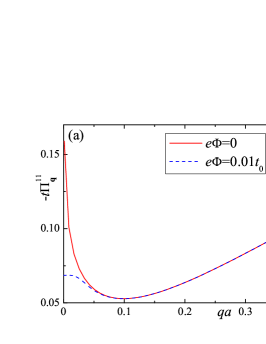
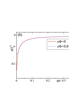
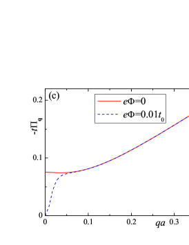
Figure 1: The polarization operator components of the undoped AB-BLG, as functions of the momentum ${\bf q}$, for $\mathbf{q}=q(1,\,0)$. Panels (a), (b), and (c) show $\Pi^{11}_{\mathbf{q}}$, $\Pi^{12}_{\mathbf{q}}$, and the total polarization operator $\Pi_{\mathbf{q}}=\sum_{ij}\Pi^{ij}_{\mathbf{q}}$, respectively. The curves in all panels are calculated for $\mu=0$. Solid (red) curves correspond to $e\Phi=0$, while dashed (blue) curves correspond to $e\Phi=0.01t_{0}$.

III polarization operator and renormalized Coulomb potential for undoped bilayer

Coulomb interaction in a solid experiences unavoidably strong renormalization due to screening. As already mentioned, we assume that the interaction function $V^{ij}_{\mathbf{q}}$ in Hamiltonian (2) incorporates static screening effects. To calculate $V^{ij}_{\mathbf{q}}$, the RPA can be used. It is commonly believed that for graphene-based systems the RPA is a more appropriate approach due to the larger degeneracy factor $N_{d}=4$.

A key element of any RPA scheme is a polarization operator. During two decades of the theoretical research on graphene numerous workers calculated the polarization operator for both biased and unbiased AB-BLG (see, e.g., Refs. Wang and Chakraborty, 2007, 2010; Lv and Wan, 2010; Hwang and Das Sarma, 2008; Sensarma et al., 2010; Gamayun, 2011; Triola and Rossi, 2012). In the most of these publications the effective two-band model of the AB-BLG has been employed. In Refs. Gamayun, 2011; Triola and Rossi, 2012 the polarization operator is calculated in the framework of four-band model using continuum approximation.

In this paper we numerically evaluate the static polarization operator $\Pi^{ij}_{\mathbf{q}}$ for the four-band tight-binding model. Both intra-layer ($i=j$) and inter-layer ($i\neq j$) components will be determined. This is to be contrasted with the majority of the previous studies that considered the total polarization operator $\Pi_{\mathbf{q}}=\sum_{ij}\Pi^{ij}_{\mathbf{q}}$ only.

The polarization operator of the undoped AB-BLG can be presented as a $2\times 2$ matrix. The elements of this matrix as functions of the transferred momentum $\mathbf{q}$ reads Triola and Rossi (2012)

$$\Pi^{ij}_{\mathbf{q}} = 2\sum_{SS^{\prime}}\int\!\frac{d^{2}\mathbf{k}}{v_{\rm BZ}}\frac{n_{\rm F}\left(\varepsilon^{(S)}_{\mathbf{k}}\right)-n_{\rm F}\left(\varepsilon^{(S^{\prime})}_{\mathbf{k}+\mathbf{q}}\right)}{\varepsilon^{(S)}_{\mathbf{k}}-\varepsilon^{(S^{\prime})}_{\mathbf{k}+\mathbf{q}}}\times$$ (10)

$$\times \Big{(}\sum_{\alpha}\Psi^{(S)}_{\mathbf{k}i\alpha}\Psi^{(S^{\prime})*}_{\mathbf{k}+\mathbf{q}i\alpha}\Big{)}\Big{(}\sum_{\beta}\Psi^{(S)*}_{\mathbf{k}j\beta}\Psi^{(S^{\prime})}_{\mathbf{k}+\mathbf{q}j\beta}\Big{)},$$

where $S,\,S^{\prime}=1,\dots,\,4$, $v_{\rm BZ}=8\pi^{2}/(a^{2}\sqrt{3})$ is the Brillouin zone area, and $n_{\rm F}(E)=[e^{(E-\mu)/T}+1]^{-1}$ is the Fermi function. We limit ourselves to zero temperature. The results of the numerical calculations of $\Pi^{ij}_{\mathbf{q}}$ are shown in Fig. 1 for two different values of $e\Phi$ ($e\Phi=0$ and $e\Phi=0.01t_{0}$).

Analyzing the numerical data we observe that $\Pi^{11}_{\mathbf{q}}=\Pi^{22}_{\mathbf{q}}$, which a manifestation of the charge-conjugation symmetry (see also Appendix A). Further, as long as $q=|\mathbf{q}|$ is not too large, $qa<1$, the polarization operator is virtually independent of the direction of $\mathbf{q}$. From Fig. 2 we see that the intra-layer components $\Pi^{11}_{\mathbf{q}}$ and $\Pi^{22}_{\mathbf{q}}$ are always negative, while $\Pi^{12}_{\mathbf{q}}$ is positive. For small $q$, the value of $-\Pi^{11}_{\mathbf{q}}$ decreases with the increase of $q$. This decay is replaced by a linear growth at larger $q$, which is similar to the behavior of the polarization operator of the single-layer graphene Kotov et al. (2012). The inter-layer polarization $\Pi^{12}_{\mathbf{q}}$ monotonously decreases with $q$. Asymptotically, it behaves as $1/q$ at $qa>0.1$.

The renormalized Coulomb interaction can be expressed in the matrix form as

$$\hat{V}_{\mathbf{q}}=\hat{V}^{(0)}_{\mathbf{q}}\left(1-\hat{\Pi}_{\mathbf{q}}\hat{V}^{(0)}_{\mathbf{q}}\right)^{-1}.$$ (11)

In this formula, the bare Coulomb interaction is a $2\times 2$ matrix

$$V^{(0)}_{\mathbf{q}}=\frac{A}{q}\left(\begin{array}[]{cc}1&e^{-qd}\\ e^{-qd}&1\end{array}\right),\;\;A=\frac{2\pi e^{2}}{{\cal S}_{\rm gr}\epsilon}\,,$$ (12)

where ${\cal S}_{\rm gr}=a^{2}\sqrt{3}/2$ is the area of the graphene unit cell, and $\epsilon$ is the dielectric constant of the media surrounding the graphene sample. Thus, we obtain

$$V^{11}_{\mathbf{q}}=V^{22}_{\mathbf{q}} = A\frac{1-\frac{A}{q}\Pi^{22}_{\mathbf{q}}[1-e^{-2qd}]}{q-A(\Pi^{11}_{\mathbf{q}}+\Pi^{22}_{\mathbf{q}}+2e^{-qd}\Pi^{12}_{\mathbf{q}})+\frac{A^{2}}{q}[\Pi^{11}_{\mathbf{q}}\Pi^{22}_{\mathbf{q}}-(\Pi^{12}_{\mathbf{q}})^{2}][1-e^{-2qd}]},$$ (13)

$$V^{12}_{\mathbf{q}}=V^{21}_{\mathbf{q}} = A\frac{e^{-qd}+\frac{A}{q}\Pi^{12}_{\mathbf{q}}[1-e^{-2qd}]}{q-A(\Pi^{11}_{\mathbf{q}}+\Pi^{22}_{\mathbf{q}}+2e^{-qd}\Pi^{12}_{\mathbf{q}})+\frac{A^{2}}{q}[\Pi^{11}_{\mathbf{q}}\Pi^{22}_{\mathbf{q}}-(\Pi^{12}_{\mathbf{q}})^{2}][1-e^{-2qd}]}.$$ (14)

Similar results can be found in the literature on the Coulomb drag in two-dimensional systems, see, for example, Refs. Kamenev and Oreg, 1995 and Flensberg et al., 1995.

At zero bias we have $\Pi^{11}_{\mathbf{q}}+\Pi^{12}_{\mathbf{q}}\neq 0$ at $q\to 0$ (which is consistent with the results obtained in Ref. Hwang and Das Sarma, 2008). Thus, the matrix $\hat{V}_{\mathbf{q}}$ is regular at $q\to 0$. In other words, the screened Coulomb potential is finite at $q=0$, which agrees with a general expectation that finite density of states at the Fermi energy leads to the suppression of the long-range Coulomb interaction.

When $e\Phi\neq 0$, the single-electron spectrum acquires a gap that affects the low-$q$ screening. Indeed, in this regime $(\Pi^{11}_{\bf q}+\Pi^{12}_{\bf q})|_{{\bf q}=0}=0$, thus, the matrix $\hat{V}_{\mathbf{q}}$ is singular at $q=0$. This singularity indicates that in the insulating state of the biased AB-BLG the long-range interaction cannot be completely screened and the resultant Coulomb potential behaves as $V^{ij}_{\mathbf{q}}\propto 1/q$ at small $q$. However, such a behavior persists for small momenta only. Additional details can be learned from Fig. 2 where numerically calculated $V^{ij}_{\mathbf{q}}$ is plotted for $e\Phi=0$ and $e\Phi=0.01t_{0}$.

Concluding this section, we would like to make the following observation. If $d\to 0$, then Eqs. (13) and (14) are replaced by one simple formula

$$V^{ij}_{\mathbf{q}}=\frac{A}{q-A\Pi_{\mathbf{q}}}.$$ (15)

The right-hand side of this expression is independent of $i$ and $j$. In other words, such an approximation implies that the inter-layer and intra-layer interactions are identical. In the literature, theoretical results essentially similar to Eq. (15) are not uncommon (see, for example, Refs. Wang and Chakraborty, 2007, 2010; Hwang and Das Sarma, 2008, to name a few). Unfortunately, the reliability of this approximation is not clear: our numerical data suggests that formula (15) is a rather crude simplification that is poorly applicable even in the limit of small $q$. More details can be found in Appendix B.

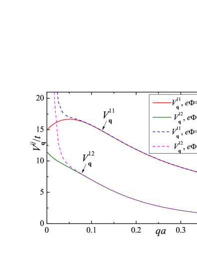
Figure 2: The renormalized interaction components as functions of the momentum $q$, at $\mathbf{q}=q(1,\,0)$, calculated for the undoped AB-BLG ($\mu=0$) and two values of the bias potential $e\Phi$. Diagonal components $V^{11}_{\mathbf{q}}=V^{22}_{\mathbf{q}}$ are plotted as red and blue curves, off diagonal $V^{12}_{\mathbf{q}}=V^{21}_{\mathbf{q}}$ components are plotted as green and magenta curves. The solid (dashed) curves represent $e\Phi=0$ case ($e\Phi=0.01t_{0}$ case). For all curves $\epsilon=1$.

IV Spin-density wave state

The computed renormalized Coulomb interaction can be applied to the study of the AB-BLG ordered states. We characterize the SDW by the following expectation value

$$\eta^{\text{SDW}}_{\mathbf{k}}=\left\langle\gamma^{{\dagger}}_{\mathbf{k}3\bar{\sigma}}\gamma^{\phantom{{\dagger}}}_{\mathbf{k}2\sigma}\right\rangle,$$ (16)

which we assumed to be independent of $\sigma$ (the bar over $\sigma$ means not $\sigma$). This relation implies that in our SDW state a hole in the band $S=2$ is coupled to an electron with opposite spin in the band $S=3$.

Equation (8) allows us to express $H_{\text{int}}$ in terms of the band operators $\gamma^{{\dagger}}_{\mathbf{k}S\sigma}$, $\gamma^{\phantom{{\dagger}}}_{\mathbf{k}S\sigma}$. Keeping only the terms relevant to the SDW pairing, one derives

$$H_{\text{int}} = -\frac{1}{2\cal N}\sum_{\mathbf{kk}^{\prime}\sigma}\left(\gamma^{{\dagger}}_{\mathbf{k}2\sigma}\gamma^{\phantom{{\dagger}}}_{\mathbf{k}3\bar{\sigma}}\Gamma^{(1)}_{\mathbf{kk}^{\prime}}\gamma^{{\dagger}}_{\mathbf{k}^{\prime}3\bar{\sigma}}\gamma^{\phantom{{\dagger}}}_{\mathbf{k}^{\prime}2\sigma}\right.+$$ (17)

$$\left.\gamma^{{\dagger}}_{\mathbf{k}2\sigma}\gamma^{\phantom{{\dagger}}}_{\mathbf{k}3\bar{\sigma}}\Gamma^{(2)}_{\mathbf{kk}^{\prime}}\gamma^{{\dagger}}_{\mathbf{k}^{\prime}2\bar{\sigma}}\gamma^{\phantom{{\dagger}}}_{\mathbf{k}^{\prime}3\sigma}+{\rm H.c.}\right),$$

where

$$\Gamma^{(1)}_{\mathbf{kk}^{\prime}} = \sum_{ij}\!\Big{(}\!\sum_{\alpha}\Psi^{(2)*}_{\mathbf{k}i\alpha}\Psi^{(2)}_{\mathbf{k}^{\prime}i\alpha}\Big{)}\!V^{ij}_{\mathbf{k}-\mathbf{k}^{\prime}}\!\Big{(}\!\sum_{\beta}\Psi^{(3)}_{\mathbf{k}j\beta}\Psi^{(3)*}_{\mathbf{k}^{\prime}j\beta}\Big{)},\;\;\;\;$$

$$\Gamma^{(2)}_{\mathbf{kk}^{\prime}} = \sum_{ij}\!\Big{(}\!\sum_{\alpha}\Psi^{(2)*}_{\mathbf{k}i\alpha}\Psi^{(3)}_{\mathbf{k}^{\prime}i\alpha}\Big{)}\!V^{ij}_{\mathbf{k}-\mathbf{k}^{\prime}}\!\Big{(}\!\sum_{\beta}\Psi^{(3)}_{\mathbf{k}j\beta}\Psi^{(2)*}_{\mathbf{k}^{\prime}j\beta}\Big{)}.\;\;\;\;$$ (18)

Note that Eq. (17) ignores retardation effects in screening physics, implying that the screening is instantaneous. The validity of this approximation will be discussed in subsection VII.2.

Introducing the SDW order parameter as

$$\Delta^{\text{SDW}}_{\mathbf{k}}=\frac{1}{\cal N}\sum_{\mathbf{k}^{\prime}}\left(\Gamma^{(1)}_{\mathbf{kk}^{\prime}}\eta^{\text{SDW}}_{\mathbf{k}^{\prime}}+\Gamma^{(2)}_{\mathbf{kk}^{\prime}}\eta^{\text{SDW}*}_{\mathbf{k}^{\prime}}\right)\,,$$ (19)

and performing the standard mean-field decoupling scheme in Eq. (17), we obtain the mean-field Hamiltonian, which allows us to calculate the grand potential $\Omega$. Minimization of $\Omega$ gives the following equation for the SDW order parameter:

$$\Delta^{\text{SDW}}_{\mathbf{k}}=\int\!\frac{d^{2}\mathbf{k}^{\prime}}{v_{\rm BZ}}\,\frac{\Gamma^{(1)}_{\mathbf{kk}^{\prime}}\Delta^{\text{SDW}}_{\mathbf{k}^{\prime}}+\Gamma^{(2)}_{\mathbf{kk}^{\prime}}\Delta^{\text{SDW}*}_{\mathbf{k}^{\prime}}}{2\sqrt{\big{[}\varepsilon^{(3)}_{\mathbf{k}^{\prime}}\big{]}^{2}+|\Delta^{\text{SDW}}_{\mathbf{k}^{\prime}}|^{2}}}.$$ (20)

Let us consider first the case of $e\Phi=0$. We do not solve the integral equation (20) directly. Instead, we perform a transparent and physically motivated approximate evaluation of $\Delta^{\text{SDW}}_{\mathbf{k}}$. First, we observe that the main contribution to the integral in the right-hand side of Eq. (20) comes from momenta $\mathbf{k}^{\prime}$ near the Dirac points $\mathbf{K}_{\xi}$ ($\xi=1,\,2$). Thus, it is necessary to know the behavior of $\Gamma^{(1)}_{\mathbf{kk}^{\prime}}$ and $\Gamma^{(2)}_{\mathbf{kk}^{\prime}}$ with momenta $\mathbf{k}$ and $\mathbf{k}^{\prime}$ close to $\mathbf{K}_{\xi}$. It is possible to show that, for $e\Phi=0$, the wave functions $\Psi^{(2,3)}_{\mathbf{k}\alpha}$ near the Dirac point $\mathbf{K}_{\xi}$ are

$$\Psi^{(2)}_{\mathbf{K}_{\xi}+\mathbf{p}i\alpha} = \frac{1}{\sqrt{2}}\left(\begin{array}[]{c}0\\ e^{-i[\frac{\pi}{2}-(-1)^{\xi}\phi_{\mathbf{p}}]}\\ e^{i[\frac{\pi}{2}-(-1)^{\xi}\phi_{\mathbf{p}}]}\\ 0\end{array}\right),$$ (25)

$$\Psi^{(3)}_{\mathbf{K}_{\xi}+\mathbf{p}i\alpha} = \frac{1}{\sqrt{2}}\left(\begin{array}[]{c}0\\ -e^{-i[\frac{\pi}{2}-(-1)^{\xi}\phi_{\mathbf{p}}]}\\ e^{i[\frac{\pi}{2}-(-1)^{\xi}\phi_{\mathbf{p}}]}\\ 0\end{array}\right),$$ (30)

where $\phi_{\mathbf{p}}$ is the polar angle of the vector $\mathbf{p}\to 0$. Substituting these equations in formulas (IV), we approximate $\Gamma^{(1,2)}_{\mathbf{K}_{\xi}+\mathbf{p}\mathbf{K}_{\xi}+\mathbf{p}^{\prime}}$ for small $|{\bf p}|$ and $|{\bf p}^{\prime}|$ as

$$\tilde{\Gamma}^{(1,2)}_{\mathbf{p}\mathbf{p}^{\prime}} \approx \frac{1}{2}\left\{V^{11}_{\mathbf{p}-\mathbf{p}^{\prime}}\pm V^{12}_{\mathbf{p}-\mathbf{p}^{\prime}}\cos\left[2(\phi_{\mathbf{p}}-\phi_{\mathbf{p}^{\prime}})\right]\right\}.$$ (31)

Here and below the tilde over a function of momentum indicates that the momentum is measured from the Dirac point $\mathbf{K}_{\xi}$. The approximate quantities $\tilde{\Gamma}^{(1,2)}_{{\bf p}{\bf p}^{\prime}}$ are the same in both valleys, consequently, dependence on $\xi$ is suppressed. Additionally, Eq. (31) implies that $\tilde{\Gamma}^{(1,2)}_{\mathbf{pp}^{\prime}}$ are real functions of momenta $\mathbf{p}$ and $\mathbf{p}^{\prime}$ when $\mathbf{p}$, $\mathbf{p}^{\prime}$ are close to a Dirac point. Therefore, one can expect that the SDW order parameter is also a real function of $\mathbf{p}$.

To estimate the SDW order parameter, we assume that $\Delta^{\text{SDW}}_{\mathbf{k}}$ is a step function of the momentum inside some region near each Dirac point, that is,

$$\Delta^{\text{SDW}}_{\mathbf{K}_{\xi}+\mathbf{p}}=\left\{\begin{array}[]{cl}\Delta^{\text{SDW}}&,\;\;|\mathbf{p}|<K_{0}\\ 0&,\;\;|\mathbf{p}|>K_{0}\end{array}\right.\,,$$ (32)

where the cutoff momentum $K_{0}$ is chosen such that the regions corresponding to different Dirac points do not intersect. Below we neglect coupling of the order parameters from different valleys and assume that $\mathbf{k}$ and $\mathbf{k}^{\prime}$ in Eq. (20) lie in the same valley. Taking $\mathbf{k}=\mathbf{K_{\xi}}$ and using the ansatz (32), one derives the equation for $\Delta^{\text{SDW}}$

$$\int\limits_{|\mathbf{p}|<K_{0}}\!\!\!\!\frac{d^{2}\mathbf{p}}{v_{\rm BZ}}\,\frac{\tilde{\Gamma}^{(1)}_{0\mathbf{p}}+\tilde{\Gamma}^{(2)}_{0\mathbf{p}}}{2\sqrt{\big{[}\tilde{\varepsilon}^{(3)}_{\mathbf{p}}\big{]}^{2}+\big{(}\Delta^{\text{SDW}}\big{)}^{2}}}=1\,.$$ (33)

We solve this equation numerically, taking $K_{0}$ by its maximum possible value $K_{0}=2\pi/(3a)$. We choose $\epsilon=1$. Other parameters are fixed as explained above. In so doing, we obtain $\Delta^{\text{SDW}}=0.0018t=4.9$ meV. This result is in agreement with experimentally available data, Ref. Veligura et al., 2012, where the measured transport gap in the Bernal bilayer graphene, which is twice of the order parameter, is equal to $\Delta_{\text{tr}}=8$ meV.

In our approach the SDW order arises due to the long-range Coulomb interaction. Thus, the result is sensitive to the value of dielectric constant: if $\epsilon$ is increased, the order parameter decreases. For example, for $\epsilon=5$, we find that $\Delta^{\rm SDW}=0.15$ meV, which is about thirty times smaller than the value of $\Delta^{\rm SDW}$ at $\epsilon=1$.

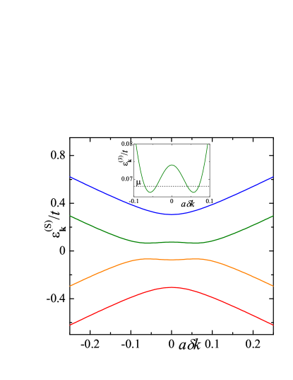
Figure 3: Band structure of the biased bilayer graphene near Dirac point, calculated at $e\Phi=0.5t_{0}$. Four bands $S=1,\ldots,4$ are plotted as functions of the deviation of momentum from the Dirac point $\delta k$. Inset shows the fine structure of the band $\varepsilon^{(3)}_{\mathbf{k}}$ close to Dirac point. Horizontal dashed line is the position of the chemical potential $\mu$.

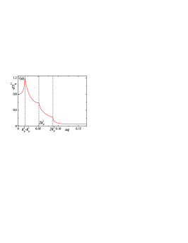
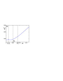
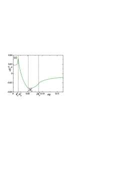
Figure 4: The polarization operator components for biased doped AB-BLG, as functions of the momentum ${\bf q}$, for $\mathbf{q}=q(1,\,0)$. Panels (a), (b), and (c) show $\Pi^{11}_{\mathbf{q}}$, $\Pi^{22}_{\mathbf{q}}$, and $\Pi^{12}_{\mathbf{q}}$, respectively. The curves in all panels are calculated for $e\Phi=0.3t_{0}$ and $\mu=0.021t$.

Consider now the case of $e\Phi\neq 0$. At finite bias, the gap between bands $2$ and $3$ arises even in the single-particle approximation. Therefore, one can expect that the bias voltage destroys the SDW ordering. Indeed, if the gap is open, the denominator in Eq. (20) never reaches zero even in the limit of $\Delta^{\text{SDW}}\to 0$. As a result, we obtain from $\Delta^{\text{SDW}}\to 0$ the following criterion for the existence of the SDW ordering at finite bias voltage

$$\int\limits_{|\mathbf{p}|<K_{0}}\!\!\!\!\frac{d^{2}\mathbf{p}}{v_{\rm BZ}}\,\frac{\tilde{\Gamma}^{(1)}_{\mathbf{p}^{\prime}\mathbf{p}}+\tilde{\Gamma}^{(2)}_{\mathbf{p}^{\prime}\mathbf{p}}}{2\tilde{\varepsilon}^{(3)}_{\mathbf{p}}}>1\,,$$ (34)

where the momentum $\mathbf{p}^{\prime}$ is to be chosen to maximize the integral. The values $V^{ij}_{\mathbf{q}}$ for $e\Phi=0$ and $e\Phi\neq 0$ almost coincide at larger ${\bf q}$ (see Fig. 2) and we assume that $e\Phi$ is small enough. Then, in Eq. (34) we can use the functions $\Gamma^{(1,2)}_{\mathbf{kk}^{\prime}}$ calculated at $e\Phi=0$ (divergence of $V^{ij}_{\mathbf{q}}$ for $e\Phi\neq 0$ at $q\to 0$ is an integrable one). In this case, one can take $\mathbf{k}=\mathbf{K}_{\xi}$, or, equivalently, $\mathbf{p}^{\prime}=0$ in Eq. (34).

Numerical analysis shows that SDW ordering is completely suppressed for $e\Phi>e\Phi_{c}$, where the critical bias value is found to be $e\Phi_{c}=0.0038t=0.025t_{0}=10$ meV at $\epsilon=1$. Thus, we obtain quite natural result that the critical bias voltage $e\Phi_{c}$ is of the order of $\Delta^{\text{SDW}}$ calculated at $e\Phi=0$.

V polarization operator and renormalized Coulomb potential for doped bilayer

The non-superconducting ordered state (for example, the SDW discussed above, or a similar phase) is expected to dominate any superconducting state in pristine graphene-based systems. Indeed, experimentally measured energy scales associated with non-superconducting ordered phases are in the range of several meV (see, for example, Refs. Mayorov et al., 2011; Velasco et al., 2012; Veligura et al., 2012; Freitag et al., 2012), while the relevant superconducting energy is several orders of magnitude lower Zhou et al. (2022). Consequently, it is necessary to suppress a non-superconducting order parameter to make a superconducting transition possible.

The suppression of the SDW by the bias voltage, considered in Sec. IV, is not suitable since it leads to a change from the SDW insulator to the band insulator. A more convenient approach is doping. Doping destroys the SDW ordering, replacing it by a metal with a well-developed Fermi surface.

The presence of a Fermi surface drastically changes the screening properties of AB-BLG. To account for these, we present here the results of our numerical calculations of the polarization operator and renormalized Coulomb potential of the doped and biased bilayer graphene. We consider an electron doping and assume that under doping only the band $S=3$ crosses the Fermi level $\mu$, while the band $S=4$ remains empty. It is also assumed that the following restriction on the chemical potential is met: $\mu_{\text{min}}<\mu<\mu_{\text{max}}$, where $\mu_{\text{min}}=e\Phi t_{0}/(2\sqrt{e^{2}\Phi^{2}+t_{0}^{2}})$ and $\mu_{\text{max}}=e\Phi/2$. In this case the Fermi surface consists of four approximately circular pockets. A pair of these, with Fermi momenta $k_{\rm F}^{(1)}$ and $k_{\rm F}^{(2)}$, are centered at Dirac point $\mathbf{K}_{1}$. An identical pair is centered at $\mathbf{K}_{2}$. Using Eq. (II) and linear expansion of $|t_{{\bf K}_{\xi}+\mathbf{k}}|\approx v_{\rm F}k$, where $v_{\rm F}=\sqrt{3}ta/2$ is the graphene Fermi velocity, we derive an expression for the Fermi momenta $k_{\rm F}^{(1)}$ and $k_{\rm F}^{(2)}$

$$k^{(1,2)}_{\rm F}\!\!=\!\frac{1}{v_{\rm F}}\!\sqrt{\frac{e^{2}\Phi^{2}}{4}\!+\!\mu^{2}\mp\sqrt{e^{2}\Phi^{2}\mu^{2}\!+\!\left(\!\mu^{2}\!-\!\frac{e^{2}\Phi^{2}}{4}\!\right)\!t_{0}^{2}}}.$$ (35)

Each inner Fermi surface is hole-like, while outer one is electron-like. Absolute values of the Fermi velocities at each Fermi surface are equal to ($s=1,\,2$)

$$v_{\rm F}^{(s)}=\frac{v_{\rm F}^{2}k_{\rm F}^{(s)}}{\mu}\left|1-\frac{e^{2}\Phi^{2}+t_{0}^{2}}{\sqrt{4\big{[}v_{\rm F}k_{\rm F}^{(s)}\big{]}^{2}\big{(}e^{2}\Phi^{2}+t_{0}^{2}\big{)}+t_{0}^{4}}}\right|.$$ (36)

When $\mu\to\mu_{\text{min}}$, these velocities vanish, $v_{\rm F}^{(s)}\to 0$, and the density of states at the Fermi level diverges. Band structure near the Dirac point $\mathbf{K}_{1}$ and typical position of the chemical potential are plotted in Fig. 3. The electron concentration (per one site ) is a function of $\mu$ and can be expressed as

$$x=\frac{1}{2}\int\frac{d^{2}\mathbf{k}}{v_{\text{BZ}}}\,\Theta\!\left(\mu-\varepsilon_{\mathbf{k}}^{(3)}\right)\approx\frac{\pi}{v_{\rm BZ}}\left[(k^{(2)}_{\rm F})^{2}-(k^{(1)}_{\rm F})^{2}\right],$$ (37)

where $\Theta(E)$ is the Heaviside step function.

The numerical analysis of Eq. (10) shows that the doping substantially modifies the polarization operator at small $q$ and the change comes mainly from the intraband term (term with $S=S^{\prime}=3$) in Eq. (10), which is zero if $\mu=0$. The bias voltage breaks the symmetry between graphene layers. As a result extra charge introduced by the doping accumulates mainly, say, in layer $1$. Thus, we have $\Pi^{11}_{\mathbf{q}}\neq\Pi^{22}_{\mathbf{q}}$. It turns out that $|\Pi^{11}_{\mathbf{q}}|\gg|\Pi^{22}_{\mathbf{q}}|\sim|\Pi^{12}_{\mathbf{q}}|$ at small $q$, that is, the screening in layer $1$ is much greater than in layer $2$. The dependencies of $\Pi^{11}_{\mathbf{q}}$, $\Pi^{22}_{\mathbf{q}}$, and $\Pi^{12}_{\mathbf{q}}$ on $q$ are shown in Fig. 4. We clearly see three Kohn anomalies located at momenta $q=k_{\rm F}^{(2)}-k_{\rm F}^{(1)}$, $q=2k_{\rm F}^{(1)}$, and $q=2k_{\rm F}^{(2)}$. Under doping, the value of $\Pi^{12}_{\mathbf{q}}$ is negative at small $q$ for a definite doping level; in this case it changes sign at some value of $q$. The polarization component $\Pi^{11}_{\mathbf{q}}$ is the main contributor to the total polarization $\Pi_{\mathbf{q}}$. The dependence of $\Pi_{\mathbf{q}}$ on $q$ computed in this work is consistent with the results obtained in the framework of four band continuum model in Ref. Triola and Rossi, 2012.

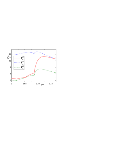
Figure 5: The renormalized interaction components at finite doping as functions of the momentum ${\bf q}$, for $\mathbf{q}=q(1,\,0)$. The curves are calculated at $e\Phi=0.3t_{0}$ and $\mu=0.0021t$. Components $V^{11}_{\mathbf{q}}$, $V^{22}_{\mathbf{q}}$, and $V^{12}_{\mathbf{q}}$ are plotted as (red) solid curve, (blue) dashed curve, and (green) dash-dotted curve, respectively. All curves are computed at $\epsilon=1$.

The typical dependence of $V^{ij}_{\mathbf{q}}$ on $q$ (for $\epsilon=1$) at finite doping and bias voltage is shown in Fig. 5. In this regime $\Pi^{11}_{\mathbf{q}}\neq\Pi^{22}_{\mathbf{q}}$, consequently, $V^{11}_{\mathbf{q}}\neq V^{22}_{\mathbf{q}}$. When $q\lesssim 2k_{\rm F}^{(2)}$, we have $V^{11}_{\mathbf{q}}\ll V^{22}_{\mathbf{q}}$. At small $q$ the screening in the layer 2 is the weakest, thus, the interaction inside this layer is the strongest. The screening effects of the carriers introduced by doping become less important for larger $q$, where $V^{11}_{\bf q}$ and $V^{22}_{\bf q}$ are of the same order.

The important feature of the curves shown in Fig. 5 is that, when $q\lesssim 2k_{\rm F}^{(2)}$, the interaction $V^{ij}_{\mathbf{q}}$ increases with $q$. As we will prove in the next section, such a behavior is sufficient to stabilize a triplet superconducting state.

VI Triplet superconductivity

The following consideration of superconductivity in biased and doped bilayer graphene assumes that the bias voltage $e\Phi$ exceeds the critical value $e\Phi_{c}$, thus, the SDW state is suppressed. The considered here type of the superconductivity arises due to Coulomb interaction. In contrast to usual BCS $s$-wave superconductivity, this phase exists only in the $p$-wave channel, as it will be discussed below.

To derive the mean-field form of the model, we rewrite the interaction Hamiltonian (2) in the form

$$H_{\text{int}}\!=\!\frac{1}{2\cal N}\!\sum_{\mathbf{kk}^{\prime}\sigma\sigma^{\prime}\atop ij\alpha\beta}d^{{\dagger}}_{\mathbf{k}i\alpha\sigma}d^{{\dagger}}_{-\mathbf{k}j\beta\sigma^{\prime}}V^{ij}_{\mathbf{k}-\mathbf{k}^{\prime}}d^{\phantom{{\dagger}}}_{-\mathbf{k}^{\prime}j\beta\sigma^{\prime}}d^{\phantom{{\dagger}}}_{\mathbf{k}^{\prime}i\alpha\sigma}\,,$$ (38)

where all contributions unimportant for the superconductivity are omitted. Substituting Eq. (8) in the formula above and keeping only terms with $S=3$, one obtains

$$H_{\text{int}}=\frac{1}{2\cal N}\sum_{\mathbf{kk}^{\prime}\sigma\sigma^{\prime}\atop ij\alpha\beta}\gamma^{{\dagger}}_{\mathbf{k}3\sigma}\gamma^{{\dagger}}_{-\mathbf{k}3\sigma^{\prime}}\Gamma_{\mathbf{kk}^{\prime}}^{\rm SC}\gamma^{\phantom{{\dagger}}}_{-\mathbf{k}^{\prime}3\sigma^{\prime}}\gamma^{\phantom{{\dagger}}}_{\mathbf{k}^{\prime}3\sigma}\,,$$ (39)

where

$$\Gamma_{\mathbf{kk}^{\prime}}^{\rm SC}=\sum_{ij}\Big{(}\sum_{\alpha}\Psi^{(3)*}_{\mathbf{k}i\alpha}\Psi^{(3)}_{\mathbf{k}^{\prime}i\alpha}\Big{)}V^{ij}_{\mathbf{k}-\mathbf{k}^{\prime}}\Big{(}\sum_{\beta}\Psi^{(3)*}_{-\mathbf{k}j\beta}\Psi^{(3)}_{-\mathbf{k}^{\prime}j\beta}\Big{)}.$$ (40)

The role of $\Gamma_{\mathbf{kk}^{\prime}}^{\rm SC}$ in the theory of the superconducting phase is analogous to the role of $\Gamma_{\mathbf{kk}^{\prime}}^{(1,2)}$ for the SDW, see Sec. IV. Similar to Eq. (17) we ignored screening retardation in Eq. (39) as well. For more discussion, see subsection VII.2.

We assume that our triplet ($p$-wave) superconducting state is characterized by the following anomalous expectation values

$$\eta^{\rm SC}_{\mathbf{k}}=\left\langle\gamma^{\phantom{{\dagger}}}_{-\mathbf{k}3\uparrow}\gamma^{\phantom{{\dagger}}}_{\mathbf{k}3\uparrow}\right\rangle=\left\langle\gamma^{\phantom{{\dagger}}}_{-\mathbf{k}3\downarrow}\gamma^{\phantom{{\dagger}}}_{\mathbf{k}3\downarrow}\right\rangle.$$ (41)

This specific choice is but one possibility among many; others are connected to Eq. (41) through unitary transformations representing O(3) rotations of electron spin. The superconducting order parameter can be defined as

$$\Delta^{\rm SC}_{\mathbf{k}}=\frac{1}{\cal N}\sum_{\mathbf{k}^{\prime}}\Gamma_{\mathbf{kk}^{\prime}}^{\rm SC}\eta^{\rm SC}_{\mathbf{k}^{\prime}}\,.$$ (42)

When momentum $\mathbf{k}$ is close to the Dirac point $\mathbf{K}_{\xi}$, the expectation value $\eta^{\rm SC}_{\mathbf{k}}$ couples electrons belonging to different valleys. Since $\eta^{\rm SC}_{\mathbf{k}}$ couples electrons with the same spin, one has

$$\eta^{\rm SC}_{-\mathbf{k}}=-\eta^{\rm SC}_{\mathbf{k}}\quad\Leftrightarrow\quad\Delta^{\rm SC}_{-\mathbf{k}}=-\Delta^{\rm SC}_{\mathbf{k}}.$$ (43)

Indeed, as the spin part of the Cooper pair wave function is even, the orbital wave function must be odd.

Performing the standard mean-field decoupling in Eq. (39) and minimizing the grand potential, we derive the zero-temperature self-consistency equation for $\Delta^{\rm SC}_{\mathbf{k}}$

$$\Delta^{\rm SC}_{\mathbf{k}}=-\int\!\frac{d^{2}\mathbf{k}^{\prime}}{v_{\rm BZ}}\,\frac{\Gamma_{\mathbf{kk}^{\prime}}^{\rm SC}\Delta^{\rm SC}_{\mathbf{k}^{\prime}}}{2\sqrt{\big{[}\varepsilon^{(3)}_{\mathbf{k}^{\prime}}-\mu\big{]}^{2}+\big{|}\Delta^{\rm SC}_{\mathbf{k}^{\prime}}\big{|}^{2}}}.$$ (44)

The minus sign in the right-hand side of the self-consistency equation is due to the repulsive Coulomb interaction. However, as we will show below the r.h.s. of Eq. (44) can be positive for the specific choice of the form of the order parameter.

The main contribution to the integral in Eq. (44) comes from the momenta $\mathbf{k}^{\prime}$ near each Dirac point. In these regions it is convenient to define

$$\tilde{\varepsilon}_{p}=\varepsilon^{(3)}_{\mathbf{K}_{\xi}+\mathbf{p}}\,,\quad$$ (45)

where

$$\tilde{\varepsilon}_{p}\!=\!\sqrt{v_{\rm F}^{2}p^{2}\!+\!\frac{e^{2}\Phi^{2}}{4}\!+\!\frac{t_{0}^{2}}{2}\!-\!\sqrt{\!v_{\rm F}^{2}p^{2}(e^{2}\Phi^{2}\!+\!t_{0}^{2})\!+\!\frac{t_{0}^{4}}{4}}}\quad$$ (46)

depends on the absolute value of the vector $\mathbf{p}$. We propose the following ansatz for $\Delta^{\rm SC}_{\mathbf{k}}$

$$\Delta^{\rm SC}_{\mathbf{K}_{\xi}+\mathbf{p}}=\left\{\begin{array}[]{cl}\tilde{\Delta}^{\rm SC}_{\xi p}\cos\phi_{\mathbf{p}}&,\;\;|\mathbf{p}|<K_{0}\\ 0&,\;\;\text{otherwise}\end{array}\right.\,.$$ (47)

where $\tilde{\Delta}^{\rm SC}_{\xi p}$ depends only on the absolute value of vector $\mathbf{p}$. We can show that near Dirac points the following relation is true

$$\Gamma_{\mathbf{K}_{\xi}+\mathbf{p}\mathbf{K}_{\xi}+\mathbf{p}^{\prime}}^{\rm SC}=\tilde{\Gamma}^{\rm SC}(p,\,p^{\prime},\,\phi_{\mathbf{p}}-\phi_{\mathbf{p}^{\prime}})$$ (48)

In this formula, the function $\tilde{\Gamma}^{\rm SC}(p,\,p^{\prime},\,\phi_{\mathbf{p}}-\phi_{\mathbf{p}^{\prime}})$ depends on the absolute values of the vectors $\mathbf{p}$ and $\mathbf{p}^{\prime}$, and the polar angle $\phi_{\mathbf{p}}-\phi_{\mathbf{p}^{\prime}}$ between them. Then, it is easy to derive

$$\int\limits_{0}^{2\pi}\frac{d\phi^{\prime}}{2\pi}\tilde{\Gamma}^{\rm SC}(p,\,p^{\prime},\,\phi_{\mathbf{p}}-\phi^{\prime})\cos\phi^{\prime}=-\cos\phi_{\mathbf{p}}W(p,\,p^{\prime})\,,$$ (49)

where the kernel $W$ is

$$W(p,\,p^{\prime})=-\int\limits_{0}^{2\pi}\frac{d\phi}{2\pi}\tilde{\Gamma}^{\rm SC}(p,\,p^{\prime},\,\phi)\cos\phi\,.$$ (50)

The value $W(p,\,p^{\prime})$ depends on the interactions $V^{ij}_{\mathbf{p}-\mathbf{p}^{\prime}}$, which in turn depend on $q=|\mathbf{p}-\mathbf{p}^{\prime}|$. The most important for us here is that, when $q$ increases from 0 to $\sim 2k_{\rm F}^{(2)}$, the functions $V^{ij}_{\mathbf{q}}$ demonstrate a growing trend (see Fig. 5). As a result, the integral $\int d\phi\tilde{\Gamma}\cos\phi$ in Eq. (50) is negative at sufficiently small $p$ and $p^{\prime}$, making $W(p,\,p^{\prime})$ positive at small $p$, $p^{\prime}$. Taking into account Eqs. (47), (48), (49), (50), and neglecting the intervalley coupling, we can rewrite the self-consistency equation (44) in the form

$$\tilde{\Delta}^{\rm SC}_{\xi p}=\frac{\pi}{v_{\rm BZ}}\int\limits_{0}^{K_{0}}p^{\prime}dp^{\prime}\,\frac{W(p,p^{\prime})\tilde{\Delta}^{\rm SC}_{\xi p^{\prime}}}{\sqrt{(\tilde{\varepsilon}_{p^{\prime}}-\mu)^{2}+(\tilde{\Delta}^{\rm SC}_{\xi p^{\prime}})^{2}}}.$$ (51)

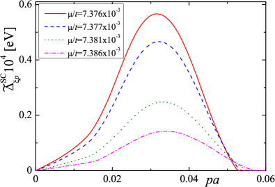
Figure 6: The dependencies of the superconducting order parameter $\tilde{\Delta}^{\rm SC}_{\xi p}$ on $p$ calculated at $e\Phi=0.1t_{0}=40$ meV and at four different values of the chemical potential (see the legend in figure). For all curves we take $\epsilon=1$.

We solve this integral equation numerically using successive iterations technique. The typical curves $\tilde{\Delta}^{\rm SC}_{\xi p}$ versus $p$, calculated for $e\Phi=0.1t_{0}=40$ meV, $\epsilon=1$, and several values of $\mu$, are plotted in Fig. 6. In this figure we observe that, as $p$ grows, the function $\tilde{\Delta}^{\rm SC}_{\xi p}$ first increases from zero, then, passing the maximum, and goes back to zero when $p\approx 4k_{\rm F}^{(2)}$. The order parameter $\tilde{\Delta}^{\rm SC}_{\xi p}$ vanishes at $p=0$ because the integral over $\phi$ in Eq. (50) is zero when $p=0$. At momenta $p\gtrsim 4k_{\rm F}^{(2)}$, we have $\tilde{\Delta}^{\rm SC}_{\xi p}=0$ because the function $W(p,\,p^{\prime})$ is negative at sufficiently large $p$ and $p^{\prime}$.

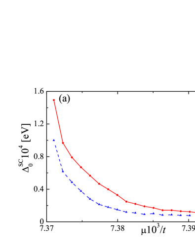
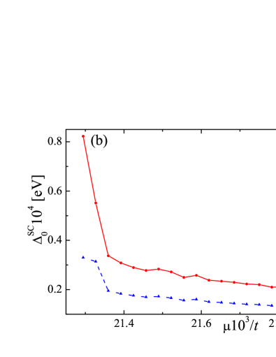
Figure 7: The dependence of the $\Delta^{\rm SC}_{0}\equiv\max(\tilde{\Delta}^{\rm SC}_{\xi p})$ on the chemical potential $\mu$ calculated for various values of the bias voltage $e\Phi$ and dielectric constant $\epsilon$. Panel (a) presents the data for $e\Phi=0.1t_{0}=40$ meV, the curves in panel (b) are plotted for $e\Phi=0.3t_{0}=120$ meV. In both panels, the (red) solid curves with filled circles correspond to $\epsilon=1$. The (blue) dashed curves with filled triangles correspond to $\epsilon=5$.

Figure 7 shows the dependence of $\Delta^{\rm SC}_{0}\equiv\max(\tilde{\Delta}^{\rm SC}_{\xi p})$ on the chemical potential. The value of $\Delta^{\rm SC}_{0}$ decreases with the increase of the chemical potential. We attribute such a behavior to the fact that the density of states at the Fermi level decreases with $\mu$. Experimental data Zhou et al. (2022) also suggests that the large density of states is crucial for the superconductivity. The data in Fig. 7 indicate that, similar to the SDW case, the superconductivity weakens when $\epsilon$ increases.

The numerical results shown in Fig. 7 demonstrate that $\Delta^{\rm SC}_{0}$ can be as large as several hundreds of mK, which exceeds by an order of magnitude the superconducting transition temperature $T_{c}=26$ mK measured experimentally Zhou et al. (2022). To reconcile the theory with the experiment, let us estimate $T_{c}$ for our model. The finite-temperature generalization of the self-consistency equation (51) was derived using a standard technique and it differs from the equation for $T=0$ only by multiplication of the function under integral by $\tanh\left[\sqrt{(\varepsilon_{p^{\prime}}-\mu)^{2}+\Delta_{\xi p^{\prime}}^{2}}/(2T)\right]$. We solve numerically the self-consistency equation for $\tilde{\Delta}^{\rm SC}_{\xi p}$ at finite temperature $T$ for several values of $\mu$ and observe a significant disparity between the order parameter and the transition temperature. For example, at $\mu/t=7.374\times 10^{-3}$, we could not find a non-trivial solution $\tilde{\Delta}^{\rm SC}_{\xi p}\neq 0$ when $T>23$ mK, which is $\approx 0.11\Delta_{0}^{\rm SC}\ll\Delta_{0}^{\rm SC}$. Therefore, for this value of $\mu$ the transition temperature is about $23$ mK, which agrees well with the experiment. We associate that “strange” feature of our model, $T_{c}\ll\Delta_{0}^{\rm SC}$, with the fact that the considered Fermi sea in the AB-BLG is very shallow: the Fermi energy defined as $\varepsilon_{\rm F}=\mu-\mu_{\text{min}}$ is comparable or even smaller than $\Delta^{\rm SC}_{0}$.

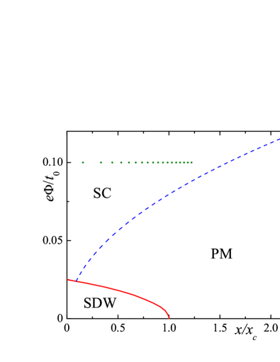
Figure 8: Schematic phase diagram of the system in the $x$ – $e\Phi$ plane. Red solid curve separates the SDW state from SC and PM states. Blue dashed curve is the curve of the crossover between the SC and PM states. The critical doping $x_{c}$ corresponding SDW to PM transition at $e\Phi=0$ is estimated as $x_{c}\approx 1.3\times 10^{-5}$ (for $t=2.7$ eV, $t_{0}=0.4$ eV, and $\epsilon=1$). Green circles depict the points ($x,\,e\Phi$) at which the superconducting order parameter was calculated numerically [see Fig. 7(a)].

All the results above can be summarized in the phase diagram of the model in the $x$ – $e\Phi$ plane. Let us consider first the SDW phase. For a given bias voltage $e\Phi$ the critical chemical potential $\mu_{c}^{\text{SDW}}$, above which the SDW state is suppressed, can be found from the equation [compare it with Eq. (34)]

$$\int\limits_{|\mathbf{p}|<K_{0}}\!\!\!\!\frac{d^{2}\mathbf{p}}{v_{\rm BZ}}\,\frac{\tilde{\Gamma}^{(1)}_{0\mathbf{p}}+\tilde{\Gamma}^{(2)}_{0\mathbf{p}}}{2\tilde{\varepsilon}^{(3)}_{\mathbf{p}}}\Theta\left(\tilde{\varepsilon}^{(3)}_{\mathbf{p}}-\mu\right)=1\,.$$ (52)

Solving this equation and using Eq. (37) we obtain the curve $x_{c}^{\text{SDW}}=x_{c}^{\text{SDW}}(e\Phi)$ separating the SDW phase from superconducting (SC) and paramagnetic (PM) phases. In connection with the SC state, we restrict ourselves by considering the chemical potentials $\mu<e\Phi/2$ when the system has two Fermi surface sheets near each Dirac point. The case of larger chemical potentials requires separate analysis. Note, however, that for $\mu>e\Phi/2$ the superconducting order parameter, even if non-zero, will be small [see Eq. (36) and the text below it]. Thus, one can consider the curve $x_{c}^{\text{SC}}(e\Phi)=x(e\Phi/2)\approx e^{2}\Phi^{2}/(2\pi\sqrt{3}t^{2})$ as the curve of the crossover between SC and PM states. The resultant phase diagram is shown in Fig. 8.

VII Discussion and conclusions

We argued above that the doped and biased Bernal stacked bilayer graphene can host Coulomb-interaction-driven triplet superconducting state. In this section we will discuss certain important details of the mechanism that remain untouched in the more formal presentation.

VII.1 Kohn-Luttinger roots of the superconductivity

The superconducting state becomes stable thanks to the fact that the functions $V^{ij}_{\mathbf{q}}$ increase with $q$ at small transferred momenta. Such a behavior of $V^{ij}_{\mathbf{q}}$ is obtained with the help of RPA. As the RPA is an uncontrollable approximation, one may wonder if our superconducting phase is indeed a genuine article, and not an artifact of careless theoretical assumptions. To such concerns we offer twofold redress. For one, the RPA validity is discussed below, see subsection VII.2.

Beside this, we argue that our mechanism of the superconductivity is not rooted in particulars of the RPA approach. Rather, one can trace its origins to the proposal Kohn and Luttinger (1965) of Kohn and Luttinger (KL). It is instructive to compare the two mechanisms. Unlike our RPA-based formalism, the classical KL calculations Kohn and Luttinger (1965) rely on the second-order perturbation theory in powers of the bare Coulomb interaction. Since the second-order correction represents screening, it reduces the electron-electron repulsion. Loosely speaking, it is a kind of attraction that counteracts the bare Coulomb repulsion. Further, this correction is singular due to the Kohn anomaly in the polarization operator. The KL paper demonstrated that, for sufficiently large Cooper pair orbital momentum, the polarization operator, being singular, overcomes the non-singular bare Coulomb interaction. In such an orbital channel effective attraction emerges, leading to the superconducting instability.

The second-order correction, as a separate theoretical object, does not occur in our formalism. However, similar to the KL idea, the role of the polarization operator is quite essential for our mechanism as well. We see that the strong screening at low $q$ dominates in the effective interaction, as attested by the curves in Fig. 5. (This is particularly true for $V^{11}$ and $V^{12}$.) The polarization operator, controlling the renormalized interaction at small $q$, causes the overall growth of the effective interactions for growing $q$ in the interval $0.025<qa<0.1$. The latter growth of $V^{ij}_{\bf q}$ is the cornerstone of the mechanism suggested in Sec. VI.

VII.2 RPA validity

Let us briefly discuss to which extent the static RPA interaction can be considered as a reliable approach for our purposes. This problem contains two sub-problems: (i) Is the RPA by itself is reliable in our situation? (ii) Is the static version of the RPA effective interaction can be used to study the SDW and superconductivity?

In connection to (i) let us consider the following. It is generally accepted that the RPA works well for phenomena involving distances greater than a characteristic screening (Debye) length $l_{D}$ Pines and Bohm (1952); Mahan (2000); Bruus and Flensberg (2004). From the data shown in Fig. 5, we can conclude that $l_{D}$ is of the order of $10\,a$, while the superconducting and SDW orders are determined mostly by the structure of the screened Coulomb interaction on the scales larger than $l_{D}$. From our numerical results it follows that the superconducting coherence length $\xi^{\textrm{SC}}\sim\hbar v_{\textrm{F}}/\Delta^{\textrm{SC}}$ is about $100\,a$ in the parameters range of interest, which is larger than $l_{D}$. Moreover, it is commonly believed that using the RPA approach is especially reasonable for the graphene-based systems since each bubble diagram enters the RPA expansion with a degeneracy factor $N_{d}=4$ (this is due to the spin and valley degeneracies) Kotov et al. (2012).

(ii) The use of static effective interaction, as expressed in Eqs. (17) and (39), is valid as long as the full dynamic polarization operator $\Pi_{\bf q}^{ij}(\omega)$ does not vary significantly over the frequency scale set by the order parameter. For the SDW phase, the order parameter is several meV. Does $\Pi_{\bf q}^{ij}(\omega)$ for the undoped AB-BLG varies strongly over this scale? To answer this question, we want to make a simple observation. The only parameters entering $\Pi_{\bf q}^{ij}(\omega)$ are $t$ and $t_{0}$, both of which are much larger than $\Delta^{\rm SDW}$. This indicates clearly that, for $\omega$ limited to the interval whose width is of order of $\Delta^{\rm SDW}$, the dynamical polarization operator may be safely approximated by its static version.

The situation with the superconducting phase requires more diligence: since the superconductivity is observed under the doping, in addition to the tunneling amplitudes, the Fermi energy enters $\Pi_{\bf q}^{ij}(\omega)$. Since $\varepsilon_{\rm F}$ is the smallest of the three energy parameters in $\Pi_{\bf q}^{ij}(\omega)$, we conclude that, when the superconducting energy scale does not exceed $\varepsilon_{\rm F}$, the static approximation works well.

VII.3 Magnetic field effect

In experiment Zhou et al. (2022) a superconducting state was observed only at finite in-plane magnetic field. This finding supports our assumption about the triplet structure of the superconducting order parameter. Indeed, it is known that the $p$-wave superconducting state, unlike its singlet counterpart, possesses a finite paramagnetic (Zeeman) susceptibility Mineev and Samokhin (1999). Consequently, the $p$-wave superconductivity is much more robust against applied magnetic field. We can speculate that, in the experiment, at finite applied field, the superconducting state replaces a non-superconducting phase that has lower zero-field energy but weaker Zeeman susceptibility. In such a scenario, application of the field can invert relative stability of the two phases, leading to the realization of the superconductivity, which is metastable at zero field.

The nature of the phase supplanted by the superconductivity is an interesting question worth further research. For example, this phase can be one of several fractional metallic states (doped SDW with spin- and valley-polarized Fermi surface), considered theoretically for graphene bilayer systems in Refs. Rakhmanov et al., 2023; Sboychakov et al., 2021. Experimental results in Ref. Zhou et al., 2022 support such a hypothesis.

VII.4 Other types of superconducting order parameter

The superconducting order parameter discussed above is not the only possible, as other types of superconductivity might be stabilized in our AB-BLG model. To illustrate this point, consider the following reasoning. The suggested above anomalous expectation $\eta^{\rm SC}_{\mathbf{k}}=\langle\gamma^{\phantom{{\dagger}}}_{-\mathbf{k}3\sigma}\gamma^{\phantom{{\dagger}}}_{\mathbf{k}3\sigma}\rangle$ couples electrons in different valleys and the total momentum of the Cooper pair is zero. One can consider another choice, when both electrons constituting a pair belong to the same valley. The corresponding expectation value is $\tilde{\eta}^{\rm SC}_{\mathbf{p}\xi}=\langle\gamma^{\phantom{{\dagger}}}_{\mathbf{K}_{\xi}-\mathbf{p}3\sigma}\gamma^{\phantom{{\dagger}}}_{\mathbf{K}_{\xi}+\mathbf{p}3\sigma}\rangle$. The total momentum of such a pair is $2\mathbf{K}_{\xi}$. Consequently, the superconducting order parameter oscillates in real space, making this state a type of pair-density wave Chen et al. (2004).

Since we limit ourselves to small doping, only one band crosses the Fermi level. The situation becomes richer at stronger doping, when two bands are partially filled. When this happens, an inter-band order parameter may be defined. It also oscillates in real space. However, absence of van Hove singularities at higher $\mu$ implies that the corresponding condensation energy is low.

In general, the valley degeneracy is a peculiar feature of the graphene-based materials, which introduces additional complications in the task of superconducting phases classification. Recent work Rozhkov et al. (2023) on the classification of non-superconducting phases in graphene bilayer demonstrated the challenges that one faces when the discrete index space grows twofold (from twofold spin degeneracy of a BCS-like models to fourfold spin-valley degeneracy of graphene-based metals). In Ref. Rozhkov et al., 2023 we offer an SU(4)-based approach to the non-superconducting-order classification that could possibly be extended to the superconducting phases, as well.

VII.5 Trigonal warping

The single-particle Hamiltonian of our model is constructed under the assumption that the inter-layer hopping occurs only between nearest-neighbor inter-layer sites located in positions $1A$ and $2B$, and more distant inter-layer hoppings are neglected. When this simplification is lifted, the low-energy electronic spectrum experiences certain modifications. For example, in the case $e\Phi=0$, if we include the hopping amplitude $t_{3}$ between nearest-neighbor sites in positions $1B$ and $2A$ (see, e.g., Ref. Rozhkov et al., 2016), two parabolic bands touching each other at the Dirac points are converted to four Dirac cones located near the Dirac points. Such a low-energy structure is called trigonal warping. Incorporation of the trigonal warping in our model alters the results in some aspects. First, it can change the estimate of the value of the SDW order parameter. Strictly speaking, Eq. (33) has a solution for arbitrary small interaction, since the integral in right-hand side of this equation diverges logarithmically when $\Delta^{\text{SDW}}_{\xi}\to 0$. If the trigonal warping is taken into account, the non-trivial solution to Eq. (33) appears only at finite interaction strength, since the density of states vanishes at zero energy. However, the analysis reveals that the interaction is rather strong, while the trigonal warping modify the electron spectrum only at energies about $1$ meV (see, e.g., Ref. Rozhkov et al., 2016), thus, we expect that the estimate for the SDW order parameter does not change substantially when the trigonal warping is accounted for.

The trigonal warping, of course, transforms the low-energy spectrum of the AB-BLG, which affects the superconducting state. We believe, however, that the trigonal warping does not change our results qualitatively. Studies of the superconducting state via the renormalized Coulomb interaction, which take into account the trigonal warping, have been reported in Refs. Jimeno-Pozo et al., 2023; Wagner et al., 2023. The characteristic critical temperatures found there are consistent with our results.

VII.6 The role of the order parameter fluctuations

In two-dimensional systems, finite-temperature fluctuations of the Goldstone modes destroy any non-Ising long-range order. Specifically, in the SDW phase Sboychakov et al. (2013) the Goldstone mode is the spin-wave excitations described by the O(3) non-linear $\sigma$ model in 2+1-dimensional space. As temperature grows, the O(3) field correlations smoothly decay. As a result, a continuous transition, expected within the mean-field framework, is replaced by a smooth crossover. It is expected that the characteristic crossover temperature $T_{*}^{\rm SDW}$ is of order of the mean field transition temperature

$$T_{*}^{\rm SDW}\sim T_{\rm MF}^{\rm SDW}\sim\Delta^{\rm SDW}.$$ (53)

This relation indicates that, for $0<T\ll\Delta^{\rm SDW}$ robust signatures of short-range SDW order must be detectable experimentally.

Now we discuss the superconducting state. Since the bilayer sample is very thin, the magnetic field screening by the superconducting currents may be neglected. In such a situation, the fluctuations of the complex phase of $\Delta^{\rm SC}$ can be described by the XY non-linear $\sigma$ model. At sufficiently large $T$ this model demonstrates the Berezinskii-Kosterlitz-Thouless transition whose critical temperature, similar to estimate (53), is of the order of the mean field critical temperature $T_{c}$.

VII.7 The role of substrate’s dielectric constant

Our calculations show that both the SDW and the superconductivity are weakened when the dielectric constant of the substrate grows. This is a straightforward consequence of the fact that both ordered states rely on the long-range Coulomb interaction. At the same time, these phases have dissimilar sensitivities to the increase of $\epsilon$. Specifically, we have seen that the growth of the dielectric constant from $\epsilon=1$ to $\epsilon=5$ suppresses the SDW order parameter by more than an order of magnitude. In contrast, the characteristic values of the superconducting order parameter decrease roughly twofold at most. This suggests that a substrate with larger dielectric constant shifts the balance between the SDW and the superconductivity in favor of the latter. Such a possibility can be tested experimentally. One must remember, however, that here we ignore short-range interactions, which are insensitive to screening but may affect the properties of the ordered states. If these contributions are indeed significant in AB-BLG, the expected effect of $\epsilon$ might be weak.

VII.8 Conclusions

In this paper we suggested a mechanism of superconductivity in the AB-BLG. This mechanism is based on the renormalized Coulomb electron-electron repulsion, and is similar in certain aspects to the Kohn-Luttinger mechanism. The superconducting state competes against the spin-density wave state, which is also stabilized by the Coulomb interaction. The superconductivity in the proposed model has a $p$-wave structure. Our estimate for the critical temperature, as well as order parameter sensitivity to the doping, is consistent with recent experiment. Likewise, in-plane magnetic field as a stabilization factor of the superconducting phase fits to the proposed theoretical framework.

Appendix A Charge-conjugation symmetry of biased undoped AB-BLG

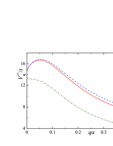
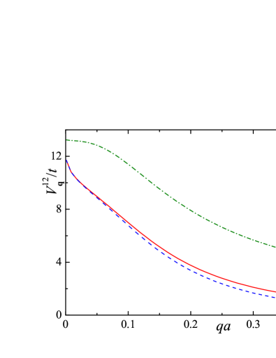
Figure 9: The renormalized interaction components $V_{\mathbf{q}}^{ij}$ as functions of $q$, calculated using different approximations; $\mathbf{q}=q(1,\,0)$, $\mu=0$, and $e\Phi=0$. Panel (a) shows $V^{11}_{\bf q}$, while panel (b) shows $V^{12}_{\bf q}$. In both panels the RPA interaction components, Eqs. (13) and (14), are plotted as (red) solid curve, approximate expressions (63) and (64) are represented by (blue) dashed curves. Dash-dotted (green) curves correspond to approximation (65). We see that Eqs. (63) and (64) work quite well for small $q$, while formula (65) is very crude approximation for our parameters choice.

Here we prove that our model is invariant under a certain charge-conjugation transformation. This invariance explains why the polarization operator components $\Pi^{11}_{\mathbf{q}}$ and $\Pi^{22}_{\mathbf{q}}$ are equal to each other as long as AB-BLG remains undoped. To start the discussion we re-write the matrix ${\cal H}_{\bf k}$ from Eq. (1) as follows

$${\cal H}_{\bf k}=\frac{e\Phi}{2}\tau_{z}-t{\bf f}\cdot\bm{\nu}$$ (54)

$$+\frac{t_{0}}{4}\left[(\nu_{x}+i\nu_{y})(\tau_{x}+i\tau_{y})+(\nu_{x}-i\nu_{y})(\tau_{x}-i\tau_{y})\right],$$

where the Pauli matrices $\nu_{i}$ act in the sublattice space, while another set of Pauli matrices $\tau_{i}$ acts in the layer space, and ${\bf f}\cdot\bm{\nu}=\nu_{x}{\rm Re}\,(f_{\bf k})-\nu_{y}{\rm Im}\,(f_{\bf k})$. For such a matrix an equality

$$\nu_{y}\tau_{x}{\cal H}_{\bf k}^{*}\nu_{y}\tau_{x}=-{\cal H}_{\bf k}$$ (55)

holds true. This relation is the signature of the charge conjugation symmetry. To reveal the invariance of $H_{0}$ under the charge conjugation, we turn our attention to the second-quantization formalism. We write

$$H_{0}=\sum_{{\bf k}\sigma}\sum_{\zeta\zeta^{\prime}}\left[{\cal H}_{\bf k}\right]_{\zeta\zeta^{\prime}}d^{\dagger}_{{\bf k}\zeta\sigma}d^{\vphantom{{\dagger}}}_{{\bf k}\zeta^{\prime}\sigma},$$ (56)

where $\left[{\cal H}_{\bf k}\right]_{\zeta\zeta^{\prime}}$ are matrix elements of ${\cal H}_{\bf k}$, and summation variables $\zeta$, $\zeta^{\prime}$ are multi-indices containing layer and sublattice labels: $\zeta=(i,\alpha)$.

If we apply a charge conjugation Bogolyubov transformation

$$d^{\vphantom{\dagger}}_{{\bf k}\zeta\sigma}\leftrightarrow d^{\dagger}_{{\bf k}\zeta\sigma},$$ (57)

the Hamiltonian $H_{0}$ transforms to

$$H^{\rm C}_{0}=\sum_{{\bf k}\sigma}\sum_{\zeta\zeta^{\prime}}\left[{\cal H}_{\bf k}\right]_{\zeta\zeta^{\prime}}d^{\vphantom{{\dagger}}}_{{\bf k}\zeta\sigma}d^{\dagger}_{{\bf k}\zeta^{\prime}\sigma}$$ (58)

$$=\sum_{{\bf k}\sigma}{\rm Tr}\,{\cal H}_{\bf k}-\sum_{{\bf k}\sigma}\sum_{\zeta\zeta^{\prime}}\left[{\cal H}_{\bf k}\right]_{\zeta\zeta^{\prime}}d^{\dagger}_{{\bf k}\zeta^{\prime}\sigma}d^{\vphantom{{\dagger}}}_{{\bf k}\zeta\sigma}$$

$$=-\sum_{{\bf k}\sigma}\sum_{\zeta\zeta^{\prime}}\left[{\cal H}_{\bf k}^{*}\right]_{\zeta\zeta^{\prime}}d^{\dagger}_{{\bf k}\zeta\sigma}d^{\vphantom{{\dagger}}}_{{\bf k}\zeta^{\prime}\sigma},$$

where we used the fact that ${\cal H}_{\bf k}$ has zero trace for any ${\bf k}$, and $\left[{\cal H}_{\bf k}\right]_{\zeta\zeta^{\prime}}=\left[{\cal H}_{\bf k}^{*}\right]_{\zeta^{\prime}\zeta}$ due to hermiticity. Thus

$$H^{\rm C}_{0} = -\sum_{\mathbf{k}\sigma}\psi^{{\dagger}}_{\mathbf{k}\sigma}{\cal H}_{\mathbf{k}}^{*}\psi^{\phantom{{\dagger}}}_{\mathbf{k}\sigma}.$$ (59)

Defining new operator vector $\psi^{\rm C}_{\mathbf{k}\sigma}$ by the relation

$$\psi^{\phantom{{\dagger}}}_{\mathbf{k}\sigma}=\nu_{y}\tau_{x}\psi^{\rm C}_{\mathbf{k}\sigma}$$ (60)

we can confirm, using Eq. (55), that $H^{\rm C}_{0}$ is unitary equivalent to $H_{0}$.

At the same time, in the first-quantization formalism, Eq. (55) implies that the transformation $\nu_{y}\tau_{x}\Psi^{(S)*}_{\bf k}$ converts the bispinor eigenvector $\Psi^{(S)}_{\bf k}$ corresponding to the energy $\varepsilon^{(S)}_{\bf k}$ into another bispinor eigenvector representing $-\varepsilon^{(S)}_{\bf k}$. Examining our definitions (II) one can check that $-\varepsilon^{(S)}_{\bf k}=\varepsilon^{(5-S)}_{\bf k}$. Thus, it is convenient to introduce the abbreviation $\bar{S}=5-S$. It allows us to write $\varepsilon^{(\bar{S})}_{\bf k}=-\varepsilon^{(S)}_{\bf k}$ and

$$\Psi^{(\bar{S})}_{{\bf k}1A}=-i\Psi^{(S)*}_{{\bf k}2B},\quad\Psi^{(\bar{S})}_{{\bf k}1B}=i\Psi^{(S)*}_{{\bf k}2A}.$$ (61)

Substituting these formulas into expression (10) for $\Pi^{11}_{\bf q}$, and exploiting the relation

$$n_{\rm F}(\varepsilon)-n_{\rm F}(\varepsilon^{\prime})=-\left[n_{\rm F}(-\varepsilon)-n_{\rm F}(-\varepsilon^{\prime})\right],$$ (62)

one can explicitly demonstrate that $\Pi^{11}_{\bf q}=\Pi^{22}_{\bf q}$.

Note that the Hamiltonian of the doped system does not possess this symmetry. Indeed, the charge conjugation inverts the sign of $\mu$, making the whole Hamiltonian non-invariant.

Appendix B Approximate expression for the screened interaction

Let us investigate here the accuracy of approximation (15). We assume that $\Pi^{11}_{\bf q}=\Pi^{22}_{\bf q}$ due to the charge-conjugation symmetry. In the limit $qd\ll 1$ we expand $\exp(-qd)\approx 1-qd$ to derive

$$V^{11}_{\mathbf{q}}=V^{22}_{\mathbf{q}}=\frac{\frac{1}{2}(1-{\cal E}\Pi^{22}_{\mathbf{q}}){\cal E}}{(qd)(1+{\cal E}\Pi^{12}_{\bf q})-{\cal E}(1+\frac{1}{2}{\cal E}\Pi^{12}_{\bf q}-\frac{1}{2}{\cal E}\Pi^{11}_{\bf q})(\Pi^{11}_{\bf q}+\Pi^{12}_{\bf q})},$$ (63)

$$V^{12}_{\mathbf{q}}=V^{21}_{\mathbf{q}}=\frac{\frac{1}{2}(1-qd+{\cal E}\Pi^{12}_{\mathbf{q}}){\cal E}}{(qd)(1+{\cal E}\Pi^{12}_{\bf q})-{\cal E}(1+\frac{1}{2}{\cal E}\Pi^{12}_{\bf q}-\frac{1}{2}{\cal E}\Pi^{11}_{\bf q})(\Pi^{11}_{\bf q}+\Pi^{12}_{\bf q})},$$ (64)

where we introduce the energy scale ${\cal E}=2Ad$. For permittivity $\epsilon=5$ one finds ${\cal E}=23.2$ eV, or, equivalently, ${\cal E}=8.6t$. This energy can be used to re-write formula (15)

$$V^{ij}_{\mathbf{q}}=\frac{\frac{1}{2}{\cal E}}{(qd)-{\cal E}(\Pi^{11}_{\mathbf{q}}+\Pi^{12}_{\mathbf{q}})}.$$ (65)

Comparing this relation and Eqs. (63) and (64), one concludes that Eq. (65) is valid only when ${\cal E}\Pi^{ij}_{\bf q}$ is much smaller than unity at small $qd$. However, for our model parameters, the quantity ${\cal E}\Pi^{ij}_{\bf q}$ is of order of unity, making Eqs. (65) and (15) a poor approximation. Figure 9 allows one to compare the accuracy of the two approximations.

References

- Cao et al. (2018a) Y. Cao, V. Fatemi, A. Demir, S. Fang, S. L. Tomarken, J. Y. Luo, J. D. Sanchez-Yamagishi, K. Watanabe, T. Taniguchi, E. Kaxiras, et al., “Correlated insulator behaviour at half-filling in magic-angle graphene superlattices,” Nature 556, 80 (2018a).
- Cao et al. (2018b) Y. Cao, V. Fatemi, S. Fang, K. Watanabe, T. Taniguchi, E. Kaxiras, and P. Jarillo-Herrero, “Unconventional superconductivity in magic-angle graphene superlattices,” Nature 556, 43 (2018b).
- Lu et al. (2019) X. Lu, P. Stepanov, W. Yang, M. Xie, M. A. Aamir, I. Das, C. Urgell, K. Watanabe, T. Taniguchi, G. Zhang, et al., “Superconductors, orbital magnets and correlated states in magic-angle bilayer graphene,” Nature 574, 653 (2019).
- Rozhkov et al. (2016) A. Rozhkov, A. Sboychakov, A. Rakhmanov, and F. Nori, “Electronic properties of graphene-based bilayer systems,” Phys. Rep. 648, 1 (2016).
- Bao et al. (2012) W. Bao, J. Velasco, F. Zhang, L. Jing, B. Standley, D. Smirnov, M. Bockrath, A. H. MacDonald, and C. N. Lau, “Evidence for a spontaneous gapped state in ultraclean bilayer graphene,” Proceedings of the National Academy of Sciences 109, 10802 (2012).
- Velasco et al. (2012) J. Velasco, L. Jing, W. Bao, Y. Lee, P. Kratz, V. Aji, M. Bockrath, C. N. Lau, C. Varma, R. Stillwell, et al., “Transport spectroscopy of symmetry-broken insulating states in bilayer graphene,” Nature Nanotechnology 7, 156 (2012).
- Veligura et al. (2012) A. Veligura, H. J. van Elferen, N. Tombros, J. C. Maan, U. Zeitler, and B. J. van Wees, “Transport gap in suspended bilayer graphene at zero magnetic field,” Phys. Rev. B 85, 155412 (2012).
- Freitag et al. (2013) F. Freitag, M. Weiss, R. Maurand, J. Trbovic, and C. Schönenberger, “Spin symmetry of the bilayer graphene ground state,” Phys. Rev. B 87, 161402 (2013).
- Nilsson et al. (2006) J. Nilsson, A. H. Castro Neto, N. M. R. Peres, and F. Guinea, “Electron-electron interactions and the phase diagram of a graphene bilayer,” Phys. Rev. B 73, 214418 (2006).
- Lang et al. (2012) T. C. Lang, Z. Y. Meng, M. M. Scherer, S. Uebelacker, F. F. Assaad, A. Muramatsu, C. Honerkamp, and S. Wessel, “Antiferromagnetism in the Hubbard Model on the Bernal-Stacked Honeycomb Bilayer,” Phys. Rev. Lett. 109, 126402 (2012).
- Wang et al. (2013) Y. Wang, H. Wang, J.-H. Gao, and F.-C. Zhang, “Layer antiferromagnetic state in bilayer graphene: A first-principles investigation,” Phys. Rev. B 87, 195413 (2013).
- Rakhmanov et al. (2023) A. L. Rakhmanov, A. V. Rozhkov, A. O. Sboychakov, and F. Nori, “Half-metal and other fractional metal phases in doped bilayer graphene,” Phys. Rev. B 107, 155112 (2023).
- Min et al. (2008) H. Min, G. Borghi, M. Polini, and A. H. MacDonald, “Pseudospin magnetism in graphene,” Phys. Rev. B 77, 041407 (2008).
- Vafek and Yang (2010) O. Vafek and K. Yang, “Many-body instability of Coulomb interacting bilayer graphene: Renormalization group approach,” Phys. Rev. B 81, 041401 (2010).
- de la Barrera et al. (2022) S. C. de la Barrera, S. Aronson, Z. Zheng, K. Watanabe, T. Taniguchi, Q. Ma, P. Jarillo-Herrero, and R. Ashoori, “Cascade of isospin phase transitions in Bernal-stacked bilayer graphene at zero magnetic field,” Nature Physics 18, 771 (2022).
- Zhou et al. (2022) H. Zhou, L. Holleis, Y. Saito, L. Cohen, W. Huynh, C. L. Patterson, F. Yang, T. Taniguchi, K. Watanabe, and A. F. Young, “Isospin magnetism and spin-polarized superconductivity in Bernal bilayer graphene,” Science 375, 774 (2022).
- Seiler et al. (2022) A. M. Seiler, F. R. Geisenhof, F. Winterer, K. Watanabe, T. Taniguchi, T. Xu, F. Zhang, and R. T. Weitz, “Quantum cascade of correlated phases in trigonally warped bilayer graphene,” Nature 608, 298 (2022).
- Chou et al. (2022a) Y.-Z. Chou, F. Wu, J. D. Sau, and S. Das Sarma, “Acoustic-phonon-mediated superconductivity in Bernal bilayer graphene,” Phys. Rev. B 105, L100503 (2022a).
- Chou et al. (2022b) Y.-Z. Chou, F. Wu, J. D. Sau, and S. Das Sarma, “Acoustic-phonon-mediated superconductivity in moiréless graphene multilayers,” Phys. Rev. B 106, 024507 (2022b).
- Szabó and Roy (2022) A. L. Szabó and B. Roy, “Competing orders and cascade of degeneracy lifting in doped Bernal bilayer graphene,” Phys. Rev. B 105, L201107 (2022).
- Jimeno-Pozo et al. (2023) A. Jimeno-Pozo, H. Sainz-Cruz, T. Cea, P. A. Pantaleón, and F. Guinea, “Superconductivity from electronic interactions and spin-orbit enhancement in bilayer and trilayer graphene,” Phys. Rev. B 107, L161106 (2023).
- Wagner et al. (2023) G. Wagner, Y. H. Kwan, N. Bultinck, S. H. Simon, and S. A. Parameswaran, “Superconductivity from repulsive interactions in Bernal-stacked bilayer graphene,” (2023), eprint arXiv:2302.00682.
- Cea (2023) T. Cea, “Superconductivity induced by the intervalley Coulomb scattering in a few layers of graphene,” Phys. Rev. B 107, L041111 (2023).
- Dong et al. (2023) Z. Dong, A. V. Chubukov, and L. Levitov, “Transformer spin-triplet superconductivity at the onset of isospin order in bilayer graphene,” Phys. Rev. B 107, 174512 (2023).
- Wang and Chakraborty (2007) X.-F. Wang and T. Chakraborty, “Coulomb screening and collective excitations in a graphene bilayer,” Phys. Rev. B 75, 041404 (2007).
- Wang and Chakraborty (2010) X.-F. Wang and T. Chakraborty, “Coulomb screening and collective excitations in biased bilayer graphene,” Phys. Rev. B 81, 081402 (2010).
- Lv and Wan (2010) M. Lv and S. Wan, “Screening-induced transport at finite temperature in bilayer graphene,” Phys. Rev. B 81, 195409 (2010).
- Hwang and Das Sarma (2008) E. H. Hwang and S. Das Sarma, “Screening, Kohn Anomaly, Friedel Oscillation, and RKKY Interaction in Bilayer Graphene,” Phys. Rev. Lett. 101, 156802 (2008).
- Sensarma et al. (2010) R. Sensarma, E. H. Hwang, and S. Das Sarma, “Dynamic screening and low-energy collective modes in bilayer graphene,” Phys. Rev. B 82, 195428 (2010).
- Gamayun (2011) O. V. Gamayun, “Dynamical screening in bilayer graphene,” Phys. Rev. B 84, 085112 (2011).
- Triola and Rossi (2012) C. Triola and E. Rossi, “Screening and collective modes in gapped bilayer graphene,” Phys. Rev. B 86, 161408 (2012).
- Kotov et al. (2012) V. N. Kotov, B. Uchoa, V. M. Pereira, F. Guinea, and A. H. Castro Neto, “Electron-Electron Interactions in Graphene: Current Status and Perspectives,” Rev. Mod. Phys. 84, 1067 (2012).
- Kamenev and Oreg (1995) A. Kamenev and Y. Oreg, “Coulomb drag in normal metals and superconductors: Diagrammatic approach,” Phys. Rev. B 52, 7516 (1995).
- Flensberg et al. (1995) K. Flensberg, B. Y.-K. Hu, A.-P. Jauho, and J. M. Kinaret, “Linear-response theory of Coulomb drag in coupled electron systems,” Phys. Rev. B 52, 14761 (1995).
- Mayorov et al. (2011) A. S. Mayorov, D. C. Elias, M. Mucha-Kruczynski, R. V. Gorbachev, T. Tudorovskiy, A. Zhukov, S. V. Morozov, M. I. Katsnelson, V. I. Fal’ko, A. K. Geim, et al., “Interaction-Driven Spectrum Reconstruction in Bilayer Graphene,” Science 333, 860 (2011).
- Freitag et al. (2012) F. Freitag, M. Weiss, R. Maurand, J. Trbovic, and C. Schönenberger, “Homogeneity of bilayer graphene,” Solid State Communications 152, 2053 (2012).
- Kohn and Luttinger (1965) W. Kohn and J. M. Luttinger, “New Mechanism for Superconductivity,” Phys. Rev. Lett. 15, 524 (1965).
- Pines and Bohm (1952) D. Pines and D. Bohm, “A Collective Description of Electron Interactions: II. Collective Individual Particle Aspects of the Interactions,” Phys. Rev. 85, 338 (1952).
- Mahan (2000) G. D. Mahan, Many-particle physics (Springer Science & Business Media, 2000).
- Bruus and Flensberg (2004) H. Bruus and K. Flensberg, Many-body quantum theory in condensed matter physics: an introduction (OUP Oxford, 2004).
- Mineev and Samokhin (1999) V. Mineev and K. Samokhin, Introduction to Unconventional Superconductivity (Taylor & Francis, Amsterdam, The Netherlands, 1999).
- Sboychakov et al. (2021) A. O. Sboychakov, A. L. Rakhmanov, A. V. Rozhkov, and F. Nori, “Bilayer graphene can become a fractional metal,” Phys. Rev. B 103, L081106 (2021).
- Chen et al. (2004) H.-D. Chen, O. Vafek, A. Yazdani, and S.-C. Zhang, “Pair Density Wave in the Pseudogap State of High Temperature Superconductors,” Phys. Rev. Lett. 93, 187002 (2004).
- Rozhkov et al. (2023) A. V. Rozhkov, A. O. Sboychakov, and A. L. Rakhmanov, “Ordering in SU(4)-symmetric model of AA bilayer graphene,” (2023), eprint arXiv:2306.05796.
- Sboychakov et al. (2013) A. O. Sboychakov, A. V. Rozhkov, A. L. Rakhmanov, and F. Nori, “Antiferromagnetic states and phase separation in doped -stacked graphene bilayers,” Phys. Rev. B 88, 045409 (2013).