Tensor-based modeling/estimation of static channels in IRS-assisted MIMO systems

Abstract

This paper proposes a tensor-based parametric modeling and estimation framework in MIMO systems assisted by intelligent reflecting surfaces (IRSs). We present two algorithms that exploit the tensor structure of the received pilot signal to estimate the concatenated channel. The first one is an iterative solution based on the alternating least squares algorithm. In contrast, the second method provides closed-form estimates of the involved parameters using the high order single value decomposition. Our numerical results show that our proposed tensor-based methods provide improved performance compared to competing state-of-the-art channel estimation schemes, thanks to the exploitation of the algebraic tensor structure of the combined channel without additional computational complexity.

I Introduction

Over the last few years, intelligent reflecting surface (IRS) has been considered one of the possible technologies to be deployed beyond fifth generation (B5G) and sixth generation (6G) wireless networks due to its potential to improve the coverage [1, 2]. An IRS is a $2$D panel composed of many passive reflecting elements whose elements are capable of independently changing the phase shifts of impinging electromagnetic waves to maximize the signal-to-noise ratio (SNR) at the intended receiver [3]. Hence, channel estimation must be performed at the end nodes of the network and the receiver should estimate the involved channels from the received pilots reflected by the IRS according to a training protocol. Several works have addressed this problem, as mentioned in [4, 5, 6, 7, 8, 9, 10, 11].

As pointed out in [4], in IRS-assisted networks channel estimation methods can be divided into structured and unstructured techniques exploiting the parametric (geometric) modeling of the cascaded channel and methods exploiting the combined channel structure, respectively. Also, in [5] a twin-IRS structure consisting of two IRSs is proposed as a way to obtain the spatial signatures of the involved channels. Also, authors in [6] propose a low-complexity channel parameter estimation that exploits the decoupling of the pilot design along the horizontal and vertical domains.

The authors in [7] propose channel parameter estimation using a low-rank PARAFAC tensor in the context of millimeter Wave (mmWave) systems. The authors in [8] use a tensor approach to perform supervised channel estimation, in which the decoupling of the BS-IRS and IRS-UE channels is achieved. Then, [9] proposes a tensor-based receiver formulated as a semi-blind problem that jointly estimates the involved channels and transmitted data. The work in [10] proposes a set of two tensor-based algorithms to do channel parameter estimation under unknown IRS hardware impairments. In our previous work [11], we propose a two-stage tensor-based framework for parametric channel parameter estimation and data detection of time-varying channels based on a $4$th order PARAFAC model.

In this paper, we propose a new signal modeling that exploits the geometric channel structure to estimate the spatial signatures of the IRS-assisted multiple input multiple output (MIMO) communication systems and formulate a $3$rd order Tucker tensor model, and derive a set of two tensor algorithms that solve the channel parameter estimation problem by either alternating least squares (ALS) or high order single value decomposition (HOSVD). Furthermore, we also study the computational complexity of the proposed schemes and selected benchmark solutions. Our simulation results show that the proposed techniques outperform the classic least squares (LS) and the state-of-the-art Khatri-Rao factorization (KRF) [8] algorithms without increasing the computational complexity.

Notation: Scalars, vectors, matrices, and tensors are represented as $a,\bm{a},\bm{A}$, and $\mathcal{A}$. Also, $\bm{A}^{*}$, $\bm{A}^{\text{T}}$, $\bm{A}^{\text{H}}$, and $\bm{A}^{\dagger}$ stand for the conjugate, transpose, Hermitian, and pseudo-inverse, of a matrix $\bm{A}$, respectively. The $j$th column of $\bm{A}\in\mathbb{C}^{I\times J}$ is denoted by $\bm{a}_{j}\in\mathbb{C}^{I\times 1}$. The operator vec$(\cdot)$ transforms a matrix into a vector by stacking its columns, e.g., $\text{vec}(\bm{A})=\bm{a}\in\mathbb{C}^{IJ\times 1}$, while the unvec$(\cdot)_{{I\times J}}$ operator undo the operation. The operator D$(\cdot)$ converts a vector into a diagonal matrix, $\text{D}_{j}(\bm{B})$ forms a diagonal matrix $R\times R$ out of the $j$th row of $\bm{B}\in\mathbb{C}^{J\times R}$. Also, $\bm{I}_{N}$ denotes an identity matrix of size $N\times N$. The symbols $\otimes$ and $\diamond$ indicate the Kronecker and Khatri-Rao products.

II System Model

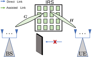
Figure 1: Proposed IRS-assisted MIMO system scenario.

We consider an uplink IRS-assisted MIMO scenario with a base station (BS) equipped with $M$ receiver antennas, which receives a signal from a user equipment (UE) equipped with $Q$ transmit antennas via a passive IRS with $N$ reflecting elements as shown in Fig. 1. The transmission has length of $T$ time-slots and the received pilot signal at the $t$-th time-slot is given by

$$\bm{y}_{t} =\bm{G}\text{D}(\bm{s}_{t})\bm{H}\bm{z}_{t}+\bm{v}_{t}\in\mathbb{C}^{M\times 1},$$ (1)

where $\bm{z}_{t}$ is the pilot sequence, $\text{D}(\bm{s}_{t})$ is the IRS phase-shift matrix, and $\bm{v}_{t}$ is the additive white Gaussian noise (AWGN) vector with $t\in\{1,\cdots,T\}$. We assume that the IRS-UE channel, $\bm{H}$, and the BS-IRS channel, $\bm{G}$, remain constant during $T$ time-slots and consider a mmWave scenario adopting a multipath channel model [12] for the involved channels. We can express these channel matrices as follows

$$\bm{G} =\sqrt{\frac{K_{G}}{K_{G}+1}}\bm{G}^{(\text{LOS})}+\sqrt{\frac{1}{K_{G}+1}}\bm{G}^{\text{(NLOS)}},$$

$$\bm{H} =\sqrt{\frac{K_{H}}{K_{H}+1}}\bm{H}^{(\text{LOS})}+\sqrt{\frac{1}{K_{H}+1}}\bm{H}^{\text{(NLOS)}},$$

with

$$\bm{G}^{(\text{LOS})} =\alpha^{(1)}\bm{a}_{\text{r}_{\text{x}}}(\mu^{(1)}_{\text{bs}})\bm{b}^{\text{(irs)}\text{H}}_{\text{t}_{\text{x}}}(\mu^{(1)}_{\text{irs}_{{\text{D}}}},\psi^{(1)}_{\text{irs}_{\text{D}}}),$$ (2)

$$\bm{G}^{(\text{NLOS})} =\sum^{L_{1}}_{l_{1}=2}\alpha^{(l_{1})}\bm{a}_{\text{r}_{\text{x}}}(\mu^{(l_{1})}_{\text{bs}})\bm{b}^{\text{(irs)}\text{H}}_{\text{t}_{\text{x}}}(\mu^{(l_{1})}_{\text{irs}_{{\text{D}}}},\psi^{(l_{1})}_{\text{irs}_{\text{D}}}),$$ (3)

$$\bm{H}^{(\text{LOS})} =\beta^{(1)}\bm{b}^{\text{(irs)}}_{\text{r}_{\text{x}}}(\mu^{(1)}_{\text{irs}_{{\text{A}}}},\psi^{(1)}_{\text{irs}_{\text{A}}})\bm{a}_{\text{t}_{\text{x}}}^{\text{H}}(\mu^{(1)}_{\text{ue}}),$$ (4)

$$\bm{H}^{(\text{NLOS})} =\sum^{L_{2}}_{l_{2}=2}\beta^{(l_{2})}\bm{b}^{\text{(irs)}}_{\text{r}_{\text{x}}}(\mu^{(l_{2})}_{\text{irs}_{{\text{A}}}},\psi^{(l_{2})}_{\text{irs}_{\text{A}}})\bm{a}_{\text{t}_{\text{x}}}^{\text{H}}(\mu^{(l_{2})}_{\text{ue}}),$$ (5)

where $\bm{G}^{(\text{LOS})}$, and $\bm{H}^{(\text{LOS})}$, are the line of sight (LOS) components and $\bm{G}^{(\text{NLOS})}$, and $\bm{H}^{(\text{NLOS})}$ are the non-line of sight (NLOS) components. Also, $K_{G}$ and $K_{H}$ are the Rician factors for channels $\bm{G}$ and $\bm{H}$. The $l$th one-dimensional steering vector of the BS is $\bm{a}_{\text{r}_{\text{x}}}(\mu^{(l_{1})}_{\text{bs}})$ having spatial frequency defined as $\mu^{(l_{1})}_{\text{bs}}=\pi\text{cos}(\phi^{(l_{1})}_{\text{bs}})$ with $\phi^{(l_{1})}_{\text{bs}}$ being the angle of arrival (AoA), which can be further written in terms of spatial frequency assuming uniform linear array (ULA) as [13]

$$\bm{a}_{\text{r}_{\text{x}}}(\mu^{(l_{1})}_{\text{bs}})=\left[1,\cdots,e^{-j\pi(M-1)\mu^{(l_{1})}_{\text{bs}}}\right]^{\text{T}}\in\mathbb{C}^{M\times 1}.$$ (6)

Similarly, the $p$th one-dimensional steering vector for the UE is $\bm{a}_{\text{t}_{\text{x}}}(\mu^{(l_{2})}_{\text{ue}})$ having spatial frequency, which is defined as $\mu^{(l_{2})}_{\text{ue}}=\pi\text{cos}(\phi^{(l_{2})}_{\text{ue}})$, with $\phi^{(l_{2})}_{\text{ue}}$ being the angle of departure (AoD), and can be written in terms of spatial frequency as

$$\bm{a}_{\text{t}_{\text{x}}}(\mu^{(l_{2})}_{\text{ue}})=\left[1,\cdots,e^{-j\pi(Q-1)\mu^{(l_{2})}_{\text{ue}}}\right]^{\text{T}}\in\mathbb{C}^{Q\times 1}.$$ (7)

At the IRS, $\bm{b}^{(\text{irs})}_{\text{r}_{\text{x}}}(\mu^{(l_{2})}_{\text{irs}_{{\text{A}}}},\psi^{(l_{2})}_{\text{irs}_{\text{A}}})$ is the 2D steering vector having spatial frequencies defined as $\mu^{(l_{2})}_{\text{irs}_{{\text{A}}}}=\pi\text{cos}(\phi^{(l_{2})}_{\text{irs}_{\text{A}}})\text{sin}(\theta^{(l_{2})}_{\text{irs}_{\text{A}}})$ and $\psi^{(l_{2})}_{\text{irs}_{\text{A}}}=\pi\text{cos}(\phi^{(l_{2})}_{\text{irs}_{\text{A}}})$, where $\phi^{(l_{2})}_{\text{irs}_{\text{A}}}$ and $\theta^{(l_{2})}_{\text{irs}_{\text{A}}}$ are the azimuth AoA and the elevation AoA, respectively. This can be further written as the Kronecker product between two steering vectors as [13]

$$\bm{b}^{\text{(irs)}}_{\text{r}_{\text{x}}}(\mu^{(l_{2})}_{\text{irs}_{{\text{A}}}},\psi^{(l_{2})}_{\text{irs}_{\text{A}}})=\bm{b}^{\text{(irs)}}_{\text{r}_{\text{x}}}(\mu^{(l_{2})}_{\text{irs}_{{\text{A}}}})\otimes\bm{b}^{\text{(irs)}}_{\text{r}_{\text{x}}}(\psi^{(l_{2})}_{\text{irs}_{\text{A}}})\in\mathbb{C}^{N\times 1}.$$ (8)

The IRS transmission steering vector, $\bm{b}^{\text{(irs)\text{H}}}_{\text{t}_{\text{x}}}(\mu^{(l_{1})}_{\text{irs}_{{\text{D}}}},\psi^{(l_{1})}_{\text{irs}_{\text{D}}})$, is defined similarly. The IRS phase-shift vector is defined as $\bm{s}_{t}=\left[e^{j\theta_{t}},\cdots,e^{j\theta_{N,t}}\right]^{\text{T}}\in\mathbb{C}^{N\times 1}$, where $\theta_{n,t}$ is the phase-shift of the $n$th IRS element at the $t$th time slot. Also, $\bm{\alpha}=\left[\alpha^{(1)},\cdots,\alpha^{(L_{1})}\right]^{\text{T}}\in\mathbb{C}^{L_{1}\times 1}$ and $\bm{\beta}=\left[\beta^{(1)},\cdots,\beta^{(L_{2})}\right]^{\text{T}}\in\mathbb{C}^{L_{2}\times 1}$ represent the path loss and fading components of the BS-IRS and IRS-UE channels, respectively. Both channels are written in matrix notation as

$$\bm{G} =\bm{A}_{\text{r}_{\text{x}}}\bm{D}(\bm{\alpha})\bm{B}^{\text{H}}_{\text{t}_{\text{x}}}\in\mathbb{C}^{M\times N},$$ (9)

$$\bm{H} =\bm{B}_{\text{r}_{\text{x}}}\bm{D}(\bm{\beta})\bm{A}_{\text{t}_{\text{x}}}^{\text{H}}\in\mathbb{C}^{N\times Q},$$ (10)

where $\bm{A}_{\text{r}_{\text{x}}}$ and $\bm{B}_{\text{r}_{\text{x}}}$ are the steering matrices defined as

$$\bm{A}_{\text{r}_{\text{x}}} =\left[\bm{a}_{\text{r}_{\text{x}}}(\mu^{(1)}_{\text{bs}}),\cdots,\bm{a}_{\text{r}_{\text{x}}}(\mu^{(L_{1})}_{\text{bs}})\right]\in\mathbb{C}^{M\times L_{1}},$$

$$\bm{B}_{\text{r}_{\text{x}}} =\left[\bm{b}^{(\text{irs})}_{\text{r}_{\text{x}}}(\mu^{(1)}_{\text{irs}_{{\text{A}}}},\psi^{(1)}_{\text{irs}_{\text{A}}}),\cdots,\bm{b}^{\text{(irs)}}_{\text{r}_{\text{x}}}(\mu^{(L_{2})}_{\text{irs}_{{\text{A}}}},\psi^{(L_{2})}_{\text{irs}_{\text{A}}})\right]\in\mathbb{C}^{N\times L_{2}},$$

with $\bm{B}_{\text{t}_{\text{x}}}$ and $\bm{A}_{\text{t}_{\text{x}}}$ being defined in similar manner.

III Pilot-based Parameter Estimation

In this section, we describe the proposed tensor-based methods for channel parameter estimation, namely Tucker-ALS as in Alg. 1, and Tucker-HOSVD as in Alg.2. The main idea is to exploit the geometric structure of the involved channels by using a tensor approach.

III-A Tensor-Based Parameter Estimation

In this section, we formulate a tensor-based approach to estimate the channel parameters. Using $\text{vec}(\bm{A}\bm{B}\bm{C})=(\bm{C}^{\text{T}}\otimes\bm{A})\text{vec}(\bm{B})$ and $\text{vec}(\bm{A}\text{D}\left(\bm{b}\right)\bm{C})=(\bm{C}^{\text{T}}\diamond\bm{A})\bm{b}$ in (1), yields

$$\bm{y}_{t} =\text{vec }(\bm{I}_{M}\bm{G}\text{D}(\bm{s}_{t})\bm{H}\bm{z}_{t})+\bm{v}_{t}\in\mathbb{C}^{M\times 1},$$

$$=(\bm{s}^{\text{T}}_{t}\otimes\bm{z}^{\text{T}}_{t}\otimes\bm{I}_{M})\text{vec}(\bm{H}^{\text{T}}\diamond\bm{G})+\bm{v}_{t}.$$

$$\bm{y}_{t} =\text{vec }(\bm{I}_{M}\bm{G}\text{D}(\bm{s}_{t})\bm{H}\bm{z}_{t})+\bm{v}_{t}\in\mathbb{C}^{M\times 1},$$

$$=(\bm{z}^{\text{T}}_{t}\otimes\bm{I}_{M})\text{vec}(\bm{G}\text{D}(\bm{s}_{t})\bm{H})+\bm{v}_{t},$$

$$=(\bm{z^{\text{T}}}_{t}\otimes\bm{I}_{M})(\bm{H}^{\text{T}}\diamond\bm{G})\bm{s}_{t}+\bm{v}_{t},$$

and, applying the first property again, we have

$$\bm{y}_{t} =\text{vec}[(\bm{z}^{\text{T}}_{t}\otimes\bm{I}_{M})(\bm{H}^{\text{T}}\diamond\bm{G})\bm{s}_{t}]+\bm{v}_{t},$$

$$=(\bm{s}^{\text{T}}_{t}\otimes\bm{z}^{\text{T}}_{t}\otimes\bm{I}_{M})\text{vec}(\bm{H}^{\text{T}}\diamond\bm{G})+\bm{v}_{t}.$$

Collecting the signals during the $T$ symbol periods yields

$$\bm{y} =\left[\bm{y}_{1}^{\text{T}},\cdots,\bm{y}_{T}^{\text{T}}\right]^{\text{T}},$$

$$=[(\bm{S}\diamond\bm{Z})^{\text{T}}\otimes\bm{I}_{M}]\text{vec}(\bm{H}^{\text{T}}\diamond\bm{G})+\bm{v},$$

$$=\bm{\Omega}\hskip 4.26773pt\bm{u}+\bm{v}\in\mathbb{C}^{MT\times 1},$$ (11)

where $\bm{S}=\left[\bm{s}_{1},\cdots,\bm{s}_{T}\right]\in\mathbb{C}^{N\times T}$, $\bm{Z}=\left[\bm{z}_{1},\cdots,\bm{z}_{T}\right]\in\mathbb{C}^{Q\times T}$ are matrices collecting the IRS phase-shifts and pilots, $\bm{\Omega}=(\bm{S}\diamond\bm{Z})^{\text{T}}\otimes\bm{I}_{M}\in\mathbb{C}^{MT\times MQN}$, $\bm{u}=\textrm{vec}(\bm{H}^{\text{T}}\diamond\bm{G})\in\mathbb{C}^{MQN\times 1}$, and $\bm{v}=\left[\bm{v}^{\text{T}}_{1},\cdots,\bm{v}^{\text{T}}_{T}\right]^{\text{T}}\in\mathbb{C}^{MT\times 1}$ is the AWGN noise term. From (11), we obtain the following LS problem

$$\bm{\hat{u}}=\underset{\bm{u}}{\text{arg min}}\left|\left|\bm{y}-\bm{\Omega}\bm{u}\right|\right|^{2}_{2},$$ (12)

where the solution requires $T\geq QN$ and is given by

$$\bm{\hat{u}} =\bm{\Omega}^{\dagger}\bm{y}\in\mathbb{C}^{MQN\times 1}.$$ (13)

Let us define $\bm{R}=\textrm{unvec}_{MQ\times N}(\bm{\hat{u}})\approx\bm{H}^{\text{T}}\diamond\bm{G}\in\mathbb{C}^{MQ\times N}$, where the approximation is exact in a noiseless scenario. Using (9) and (10), while applying property $(\bm{AC})\diamond(\bm{BD})=(\bm{A}\otimes\bm{B})(\bm{C}\diamond\bm{D})$, we have

$$\bm{R} \approx[\bm{A}_{\text{t}_{\text{x}}}^{*}\text{D}(\bm{\beta})\bm{B}^{\text{T}}_{\text{r}_{\text{x}}}]\diamond[\bm{A}_{\text{r}_{\text{x}}}\text{D}(\bm{\alpha})\bm{B}^{\text{H}}_{\text{t}_{\text{x}}}],$$

$$\approx(\bm{A}_{\text{t}_{\text{x}}}^{*}\otimes\bm{A}_{\text{r}_{\text{x}}})[\text{D}(\bm{\beta})\otimes\text{D}(\bm{\alpha})](\bm{B}^{\text{T}}_{\text{r}_{\text{x}}}\diamond\bm{B}^{\text{H}}_{\text{t}_{\text{x}}}).$$ (14)

Defining $\bm{f}=\bm{\beta}\otimes\bm{\alpha}\in\mathbb{C}^{L_{1}L_{2}\times 1}$, (14) can be expressed as

$$\bm{R} \approx(\bm{A}_{\text{t}_{\text{x}}}^{*}\otimes\bm{A}_{\text{r}_{\text{x}}})\text{D}(\bm{f})\bm{P}^{\text{T}}_{B}\in\mathbb{C}^{MQ\times N},$$ (15)

where $\bm{P}_{B}=(\bm{B}^{\text{T}}_{\text{r}_{\text{x}}}\diamond\bm{B}^{\text{H}}_{\text{t}_{\text{x}}})\in\mathbb{C}^{N\times L_{1}L_{2}}$ is the IRS geometry information. Note that $\text{D}(\bm{f})\in\mathbb{C}^{L_{1}L_{2}\times L_{1}L_{2}}$ can be viewed as the $3$-mode unfolding of the tensor $\mathcal{F}\in\mathbb{C}^{L_{1}\times L_{2}\times L_{1}L_{2}}$, i.e., $\text{D}(\bm{f})=\left[\mathcal{F}\right]_{(3)}$. The tensor $\mathcal{F}$ is given by [14]

$$\mathcal{F} =\left(\mathcal{I}_{3,L_{2}}\otimes^{2,3}_{2,3}\mathcal{I}_{3,L_{1}}\right)\times_{3}\bm{f}^{\text{T}}\in\mathbb{C}^{L_{1}\times L_{2}\times L_{1}L_{2}},$$ (16)

where $\mathcal{I}_{3,L_{2}}$ and $\mathcal{I}_{3,L_{1}}$ are identity tensors and $\otimes^{2,3}_{2,3}$ is the selective Kronecker product (SKP) [14], from which we arranged (15) following a third-way Tucker tensor structure $\mathcal{R}\in\mathbb{C}^{M\times Q\times N}$, as shown in Fig. 2, in terms of $n$-mode product as

$$\mathcal{R} \approx\mathcal{F}\times_{1}\bm{A}_{\text{r}_{\text{x}}}\times_{2}\bm{A}^{*}_{\text{t}_{\text{x}}}\times_{3}\bm{P}_{B},$$ (17)

with the matrix unfoldings of $\mathcal{R}$ given by

$$\left[\mathcal{R}\right]_{(1)} \approx\bm{A}_{\text{r}_{\text{x}}}\left[\mathcal{F}\right]_{(1)}(\bm{P}_{B}\otimes\bm{A}^{*}_{\text{t}_{\text{x}}})^{\text{T}}\in\mathbb{C}^{M\times QN},$$

$$\left[\mathcal{R}\right]_{(2)} \approx\bm{A}^{*}_{\text{t}_{\text{x}}}\left[\mathcal{F}\right]_{(2)}(\bm{P}_{B}\otimes\bm{A}_{\text{r}_{\text{x}}})^{\text{T}}\in\mathbb{C}^{Q\times MN},$$

$$\left[\mathcal{R}\right]_{(3)} \approx\bm{P}_{B}\left[\mathcal{F}\right]_{(3)}(\bm{A}^{*}_{\text{t}_{\text{x}}}\otimes\bm{A}_{\text{r}_{\text{x}}})^{\text{T}}\in\mathbb{C}^{N\times MQ}.$$

Consequently, the estimation of $\bm{A}_{\text{r}_{\text{x}}}$, $\bm{A}_{\text{t}_{\text{x}}}$, $\bm{P}_{B}$ and $\mathcal{F}$ consists of solving the following problem

$$\left\{\hat{\bm{A}}_{\text{r}_{\text{x}}},\hat{\bm{A}}_{\text{t}_{\text{x}}},\hat{\bm{P}_{B}},\hat{\mathcal{F}}\right\}=\underset{\bm{A}_{\text{r}_{\text{x}}},\bm{A}_{\text{t}_{\text{x}}},\bm{P}_{B},\mathcal{F}}{\text{arg min}}\left|\left|\begin{split}\mathcal{R}-\mathcal{F}\times_{1}\bm{A}_{\text{r}_{\text{x}}}\\ \times_{2}\bm{A}^{*}_{\text{t}_{\text{x}}}\times_{3}\bm{P}_{B}\end{split}\right|\right|^{2}_{\text{F}},$$ (18)

which can be performed by means of the well-known ALS algorithm [15] or the HOSVD algorithm [16].

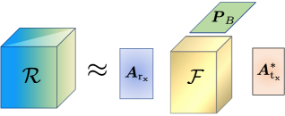
Figure 2: Proposed Tucker-based model.

III-B Tucker ALS

From (17) we can derive an iterative solution based on the well-known ALS algorithm [15]. Here, the algorithm consists of an estimate $\bm{A}_{\text{r}_{\text{x}}}$, $\bm{A}_{\text{t}_{\text{x}}}$, $\bm{P}_{B}$, and $\mathcal{F}$ in an alternating way by iteratively solving the following cost functions

$$\hat{\bm{A}}_{\text{r}_{\text{x}}} =\underset{\bm{A}_{\text{r}_{\text{x}}}}{\text{arg min}}\left|\left|\left[\mathcal{R}\right]_{(1)}-\bm{A}_{\text{r}_{\text{x}}}\left[\mathcal{F}\right]_{(1)}(\bm{P}_{B}\otimes\bm{A}^{*}_{\text{t}_{\text{x}}})^{\text{T}}\right|\right|^{2}_{\text{F}},$$ (19)

$$\hat{\bm{A}}_{\text{t}_{\text{x}}} =\underset{\bm{A}_{\text{t}_{\text{x}}}}{\text{arg min}}\left|\left|\left[\mathcal{R}\right]_{(2)}-\bm{A}^{*}_{\text{t}_{\text{x}}}\left[\mathcal{F}\right]_{(2)}(\bm{P}_{B}\otimes\bm{A}_{\text{r}_{\text{x}}})^{\text{T}}\right|\right|^{2}_{\text{F}},$$ (20)

$$\hat{\bm{P}}_{B} =\underset{\bm{P}_{B}}{\text{arg min}}\left|\left|\left[\mathcal{R}\right]_{(3)}-\bm{P}_{B}\left[\mathcal{F}\right]_{(3)}(\bm{A}^{*}_{\text{t}_{\text{x}}}\otimes\bm{A}_{\text{r}_{\text{x}}})^{\text{T}}\right|\right|^{2}_{\text{F}},$$ (21)

$$\hat{\bm{f}} =\underset{\bm{f}}{\text{arg min}}\left|\left|\text{vec}(\left[\mathcal{R}\right]_{(3)})-[(\bm{A}^{*}_{\text{t}_{\text{x}}}\otimes\bm{A}_{\text{r}_{\text{x}}})\diamond\bm{P}_{B}]\bm{f}\right|\right|^{2}_{2},$$ (22)

where $\bm{f}$ is related to the diagonal elements of $\left[\mathcal{F}\right]_{(3)}$ and its expression is derived by applying $\text{vec}(\bm{A}\text{D}\left(\bm{b}\right)\bm{C})=(\bm{C}^{\text{T}}\diamond\bm{A})\bm{b}$ to $\left[\mathcal{R}\right]_{(3)}$. The solutions for (19)-(22) are respectively given by

$$\hat{\bm{A}}_{\text{r}_{\text{x}}} =\left[\mathcal{R}\right]_{(1)}\left[\left[\mathcal{F}\right]_{(1)}(\bm{P}_{B}\otimes\bm{A}^{*}_{\text{t}_{\text{x}}})^{\text{T}}\right]^{\dagger},$$ (23)

$$\hat{\bm{A}}_{\text{t}_{\text{x}}} =\left[\mathcal{R}\right]_{(2)}\left[\left[\mathcal{F}\right]_{(2)}(\bm{P}_{B}\otimes\bm{A}_{\text{r}_{\text{x}}})^{\text{T}}\right]^{\dagger},$$ (24)

$$\hat{\bm{P}}_{B} =\left[\mathcal{R}\right]_{(3)}\left[\left[\mathcal{F}\right]_{(3)}(\bm{A}^{*}_{\text{t}_{\text{x}}}\otimes\bm{A}_{\text{r}_{\text{x}}})^{\text{T}}\right]^{\dagger},$$ (25)

$$\hat{\bm{f}} =\left[(\bm{A}^{*}_{\text{t}_{\text{x}}}\otimes\bm{A}_{\text{r}_{\text{x}}})\diamond\bm{P}_{B}\right]^{\dagger}\text{vec}(\left[\mathcal{R}\right]_{(3)}),$$ (26)

with each solution requiring that $QN\geq L_{1}$, $MN\geq L_{2}$, $MQ\geq L_{1}L_{2}$, and $NMQ\geq L_{1}L_{2}$. These four conditions are related to the convergence of the LS estimates $\bm{A}_{\text{r}_{\text{x}}}$, $\bm{A}^{*}_{\text{t}_{\text{x}}}$, $\bm{P}_{B}$, and $\bm{f}$, respectively. The proposed ALS algorithm consists of four iterative and alternating update steps that follow the LS solutions (23)-(26). At each update, the reconstruction error is minimized according to one given factor matrix by fixing the other matrices to their estimation obtained at the previous update. This procedure is repeated until the convergence is acknowledged, which happens when the reconstruction error, given by $e(i)=||\mathcal{R}-\hat{\mathcal{R}}(i)||^{2}_{\text{F}}$, achieves $||e(i)-e(i-1)||\leq\epsilon$ and $\epsilon$ is the threshold parameter with $\hat{\mathcal{R}}(i)$ being the reconstruct tensor model at the $i$th iteration. In this work, we initialize the factor matrices randomly and the convergence threshold is set to $\epsilon=10^{-5}$. It is worth noting that our solution using the ALS is not unique although, after the convergence, the intrinsic scaling and permutation ambiguities disappear on the estimated tensor model $\hat{\mathcal{R}}=\hat{\mathcal{F}}\times_{1}\hat{\bm{A}}_{\text{r}_{\text{x}}}\times_{2}\hat{\bm{A}}^{*}_{\text{t}_{\text{x}}}\times_{3}\hat{\bm{P}}_{B}$.

Algorithm 1 ALS

1:Tensor $\mathcal{R}$

2:while $||e(i)-e(i-1)||\geq\delta$ do

3:    Find a LS estimate of $\bm{A}_{\text{r}_{\text{x}}}$ with (23).

4:    Find a LS estimate of $\bm{A}_{\text{t}_{\text{x}}}$ with (24).

5:    Find a LS estimate of $\bm{P}_{B}$ with (25).

6:    Find an estimate of $\bm{f}$ with (26).

7:    Build $\mathcal{F}$ with (16).

8:    Repeat until convergence.

9:end while

10:return $\hat{\mathcal{R}}=\hat{\mathcal{F}}\times_{1}\hat{\bm{A}}_{\text{r}_{\text{x}}}\times_{2}\hat{\bm{A}}^{*}_{\text{t}_{\text{x}}}\times_{3}\hat{\bm{P}}_{B}$

III-C Tucker HOSVD

Considering the Tucker model in (17), we can also estimate its factors by finding a multi-linear rank ($L_{1},L_{2},L_{1}L_{2}$) approximation to $\mathcal{R}$. This can be done by means of the state-of-art truncated HOSVD algorithm. This algorithm consists of computing multiple singular value decompositions (SVDs), one for each unfolding of $\mathcal{R}$, as follows

$$\left[\mathcal{R}\right]_{(1)} =\bm{U}^{(1)}\bm{\Sigma}^{(1)}\bm{V}^{(1)\text{H}},$$ (27)

$$\left[\mathcal{R}\right]_{(2)} =\bm{U}^{(2)}\bm{\Sigma}^{(2)}\bm{V}^{(2)\text{H}},$$ (28)

$$\left[\mathcal{R}\right]_{(3)} =\bm{U}^{(3)}\bm{\Sigma}^{(3)}\bm{V}^{(3)\text{H}}.$$ (29)

The estimates of the steering matrices $\bm{A}_{\text{r}_{\text{x}}}$, $\bm{A}_{\text{t}_{\text{x}}}$, and $\bm{P}_{B}$ are found from the dominant $L_{1}$, $L_{2}$, and $L_{1}L_{2}$ left singular vectors of $\left[\mathcal{R}\right]_{(1)}$, $\left[\mathcal{R}\right]_{(2)}$, and $\left[\mathcal{R}\right]_{(3)}$, respectively

$$\hat{\bm{A}}_{\text{r}_{\text{x}}}=\bm{U}^{(1)}_{.1:L_{1}},\hat{\bm{A}}_{\text{t}_{\text{x}}}=\bm{U}^{(2)}_{.1:L_{2}},\hat{\bm{P}}_{B}=\bm{U}^{(3)}_{.1:L_{1}L_{2}}.$$ (30)

Finally, an estimate of the core tensor in (17) is obtained as

$$\hat{\bm{f}} =\left[(\hat{\bm{A}}^{*}_{\text{t}_{\text{x}}}\otimes\hat{\bm{A}}_{\text{r}_{\text{x}}})\diamond\hat{\bm{P}}_{B}\right]^{\dagger}\text{vec}(\left[\mathcal{R}\right]_{(3)}),$$ (31)

where $\bm{f}$. Similar to the ALS solution, the HOSVD is not unique once any transformation applied to the core tensor does not change the tensor fit [16] except in the case where the core tensor is known [17].

Algorithm 2 Tucker HOSVD

1:Tensor $\mathcal{R}$

2:Define the singular value decomposition (SVD)s of $\left[\mathcal{R}\right]_{(1)}$, $\left[\mathcal{R}\right]_{(2)}$, and $\left[\mathcal{R}\right]_{(3)}$ with (27)-(29).

3:Compute the estimation of matrices $\bm{A}_{\text{r}_{\text{x}}}$, $\bm{A}_{\text{t}_{\text{x}}}$, and $\bm{P}_{B}$ with (30).

4:Compute the estimation of $\bm{f}=\text{vec}(\mathcal{F})$ with (31)

5:Reconstruct $\hat{\mathcal{F}}$ with (16).

6:return $\hat{\mathcal{R}}=\hat{\mathcal{F}}\times_{1}\hat{\bm{A}}_{\text{r}_{\text{x}}}\times_{2}\hat{\bm{A}}^{*}_{\text{t}_{\text{x}}}\times_{3}\hat{\bm{P}}_{B}$

III-D Computational Complexity

In Table LABEL:tab:complexity, we describe the computational complexity for the selected benchmark algorithms, LS (13) and KRF [8], and our proposed solutions, ALS and HOSVD. Consider that the pseudo-inverse of a matrix $\bm{A}\in\mathbb{C}^{I\times J}$, with $I>J$, and its rank-$R$ SVD approximation have complexities $\mathcal{O}(IJ^{2})$ and $\mathcal{O}(IJR)$, respectively. Since the design of $\bm{\Omega}$ at (13) is orthogonal, we have $\bm{\Omega}^{\dagger}=\bm{\Omega}^{\text{H}}$ which lower the cost of the pseudo-inverse computation. The KRF [8] estimates the combined channel, $\bm{R}=\bm{H}^{\text{T}}\diamond\bm{G}$, by finding estimates of both $\bm{G}$ and $\bm{H}$ that solves a set of $N$ rank-one approximations using the SVD. Regarding the proposed algorithms, the ALS computes $4$ pseudo-inverses (23)-(26) along $\text{\acs{ALS}}_{\text{iter}}$ iterations until convergence, while the HOSVD involves $3$ SVDs (27)-(29) and a pseudo-inverse (31).

IV Simulation Results

We evaluate the performance of the proposed tensor-based algorithm by comparing it with the reference parameter estimation method based on the KRF [8]. The pilot matrix $\bm{Z}\in\mathbb{C}^{Q\times T}$ is designed as a Hadamard matrix, while a discrete Fourier transform (DFT) is adopted for the IRS phase-shift matrix $\bm{S}$. The angular parameters $\phi^{(l_{1})}_{\text{bs}}$ and $\phi^{(l_{2})}_{\text{ue}}$ are randomly generated from a uniform distribution between $[-\pi,\pi]$ while the IRS elevation and azimuth angles of arrival and departure are randomly generated from a uniform distribution between $[-\pi/2,\pi/2]$. The fading coefficients $\bm{\alpha}$ and $\bm{\beta}$ are modeled as independent Gaussian random variables $\mathcal{CN}(0,1)$. The parameter estimation accuracy is evaluated in terms of the normalized mean square error (NMSE) given by

$$\text{\acs{NMSE}}(\bm{R})=\mathbb{E}\left\{\frac{\left|\left|\bm{R}^{(m)}-\hat{\bm{R}}^{(m)}\right|\right|^{2}_{\text{F}}}{\left|\left|\bm{R}^{(m)}\right|\right|^{2}_{\text{F}}}\right\},$$

with $\bm{R}=(\bm{H}^{\text{T}}\diamond\bm{G})$ being the estimated channel at the $m$th experiment, $M=10^{4}$ being the number of Monte Carlo experiments, and $\sigma^{2}_{\bm{V}}$ is the noise variance. Unless otherwise stated, the training SNR is $30$ dB, the Rician factor of the LOS channel is $K_{G}=10$ dB, and the Rician factor of the NLOS channel is $K_{H}=-10$ dB. At Figs. 4, 4, and 7 we assume $\{M=4,Q=4,L_{1}=1,L_{2}=4,N=16,\text{ and }T=64\}$, at Fig. 6 we assume $\{M=8,Q=8,N=16,\text{ and }T=128\}$, and finally at Fig. 6 we assume $\{M=8,Q=8,L_{1}=2,L_{2}=2,\text{ and }T=8N\}$.

In Fig. 4, we show the impact of the Rician factors, $K_{G}$ and $K_{H}$, on the NMSE performance associated with the estimation of the combined channel $\bm{R}=\bm{H}^{\text{T}}\diamond\bm{G}$, for the proposed algorithms and the benchmark KRF [8]. The performance improvements with increasing values of the Rician factor come from the fact that as $K_{G}$ and $K_{H}$ increases, both channels are dominated by a LOS component, which happens because the channel approaches a unitary rank and the noise rejection coming from the SVD. We can also see that the proposed algorithms outperform the classic LS (13) and the state-of-the-art KRF [8] algorithms by approximately $10$ dB and $5$ dB, respectively. Moreover, the ALS performance is better than that of the HOSVD in about 1 dB. In Fig. 4, we evaluate the NMSE performance as a function of the training SNR and verify the same gains as the evaluation of the NMSE in terms of the Rician factors. In all considered methods, we observe that the NMSE decreases with SNR linearly.

In Fig. 6, we evaluate the number of iterations required by the proposed ALS algorithm to converge as a function of the SNR for a varying number of paths, $L_{1}$ and $L_{2}$. In this figure, we define $\epsilon=10^{-5}$ as the target convergence criterion, meaning that the algorithm convergence is declared when the error between consecutive iterations is less than $\epsilon$. As expected, in the low SNR region the ALS algorithm takes more iterations to achieve convergence as the total number of components, i.e., the product $L_{1}L_{2}$, increases. At the high SNR region, the required number of iterations is the same. In Fig. 6, we observe that, as the number of reflecting elements $N$ increases, fewer iterations are needed for convergence. This is linked to LS (13) since, if $N$ increases, we sense the channel longer because of condition $T\geq QN$.

In Fig. 7, we analyze the computational complexity of the benchmark algorithms, LS (13) and KRF [8], and the proposed algorithms, ALS and HOSVD, for fixed parameters $M,Q,L_{1},L_{2}$ while varying $N$ according to Table LABEL:tab:complexity. To compute the cost of the KRF [8], the ALS, and the HOSVD, we take into account the extra cost of the LS (13) step, which is the most complex operation of the competing and our proposed solutions (see Table LABEL:tab:complexity). We observe that the competing LS and KRF [8] algorithms have approximately the same cost as the proposed ALS and HOSVD solutions.

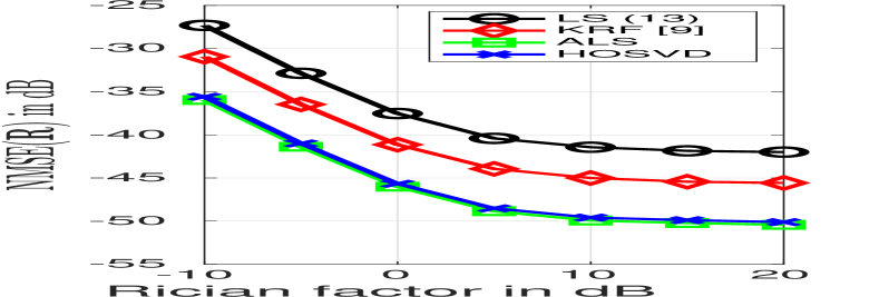
Figure 3: NMSE as a function of the Rician factors $K_{G}$ and $K_{H}$.

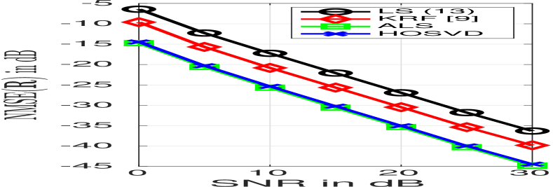
Figure 4: NMSE as a function of the training SNR.

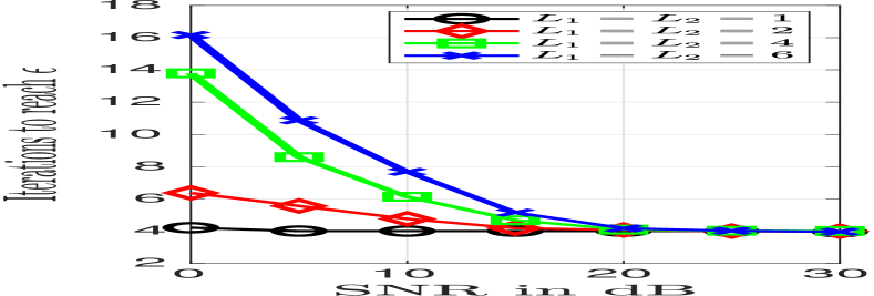
Figure 5: Iterations to converge as function of the SNR and for increasing $L_{1}$ and $L_{2}$.

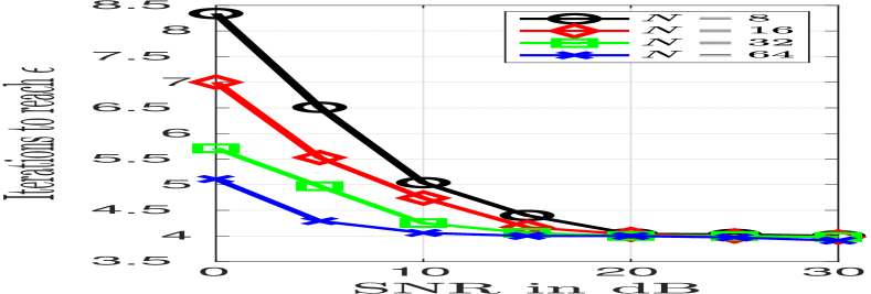
Figure 6: Iterations to converge as function of the SNR and for increasing $N$.

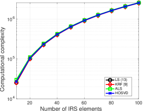
Figure 7: Computational complexity of the proposed solutions and the benchmark algorithms LS (13) KRF [8].

V Conclusions

This paper proposes two tensor-based channel parameter estimation algorithms in IRS-aided MIMO communications. From our simulation results, we observed that proposed ALS and HOSVD algorithms outperform both the classic LS and the state-of-the-art KRF algorithms in terms of NMSE by approximately $10$ dB and $5$ dB, respectively. The performance gap between the proposed solutions is small with the ALS algorithm having the best performance in terms of NMSE only. Regarding the computational complexity, the proposed ALS and HOSVD solutions have approximately the same complexity as the benchmark ones, namely, the LS (13) and the KRF [8] methods.

References

- [1] N. Rajatheva and et al., “Scoring the terabit/s goal: Broadband connectivity in 6G,” 2020, arXiv:2008.07220.
- [2] B. Zheng, C. You, W. Mei, and R. Zhang, “A survey on channel estimation and practical passive beamforming design for intelligent reflecting surface aided wireless communications,” IEEE Commun. Surv. Tutor., vol. 24, no. 2, pp. 1035–1071, 2022.
- [3] S. Gong, X. Lu, D. T. Hoang, D. Niyato, L. Shu, D. I. Kim, and Y.-C. Liang, “Toward smart wireless communications via intelligent reflecting surfaces: A contemporary survey,” IEEE Commun. Surv. Tutor., vol. 22, no. 4, pp. 2283–2314, 2020.
- [4] C. Pan, G. Zhou, K. Zhi, S. Hong, T. Wu, Y. Pan, H. Ren, M. Di Renzo, A. L. Swindlehurst, R. Zhang, et al., “An overview of signal processing techniques for RIS/IRS-aided wireless systems,” IEEE J. Sel. Topics Signal Processing, vol. 16, no. 5, pp. 883–917, 2022.
- [5] Y. Lin, S. Jin, M. Matthaiou, and X. You, “Channel estimation and user localization for IRS-assisted MIMO-OFDM systems,” IEEE Transactions on Wireless Communications, vol. 21, no. 4, pp. 2320–2335, 2021.
- [6] Fazal-E-Asim, A. L. F. de Almeida, B. Sokal, B. Makki, and G. Fodor., “Two-dimensional channel parameter estimation for IRS-assisted networks,” 2023, arXiv:2305.04393.
- [7] X. Zheng, P. Wang, J. Fang, and H. Li, “Compressed channel estimation for IRS-assisted millimeter wave OFDM systems: A low-rank tensor decomposition-based approach,” IEEE Wireless Communications Letters, vol. 11, no. 6, pp. 1258–1262, 2022.
- [8] G. T. de Araújo, A. L. de Almeida, and R. Boyer, “Channel estimation for intelligent reflecting surface assisted MIMO systems: A tensor modeling approach,” IEEE J. Sel. Top. Signal Process, vol. 15, no. 3, pp. 789–802, 2021.
- [9] G. T. de Araújo, P. R. Gomes, A. L. de Almeida, G. Fodor, and B. Makki, “Semi-blind joint channel and symbol estimation in IRS-assisted multi-user MIMO networks,” IEEE Wireless Commun. Lett., 2022.
- [10] P. R. B. Gomes, G. T. d. Araújo, B. Sokal, A. L. F. d. Almeida, B. Makki, and G. Fodor, “Channel estimation in RIS-assisted MIMO systems operating under imperfections,” IEEE Transactions on Vehicular Technology, pp. 1–14, 2023.
- [11] K. B. A. Benicio, A. L. F. de Almeida, B. Sokal, Fazal-E-Asim, B. Makki, and G. Fodor., “Tensor-based channel estimation and data-aided tracking in IRS-assisted MIMO systems,” 2023, arXiv:2305.10499.
- [12] R. W. Heath, N. Gonzalez-Prelcic, S. Rangan, W. Roh, and A. M. Sayeed, “An overview of signal processing techniques for millimeter wave MIMO systems,” IEEE J. Sel. Top. Signal Process, vol. 10, no. 3, pp. 436–453, 2016.
- [13] Fazal-E-Asim, F. Antreich, C. C. Cavalcante, A. L. F. de Almeida, and J. A. Nossek, “Two-dimensional channel parameter estimation for millimeter-wave systems using butler matrices,” IEEE Trans. Wireless Commun., vol. 20, no. 4, pp. 2670–2684, 2021.
- [14] B. Sokal, P. R. Gomes, A. L. de Almeida, and M. Haardt, “Tensor-based receiver for joint channel, data, and phase-noise estimation in MIMO-OFDM systems,” IEEE J. Sel. Top. Signal Process, vol. 15, no. 3, pp. 803–815, 2021.
- [15] P. Comon, X. Luciani, and A. L. de Almeida, “Tensor decompositions, alternating least squares and other tales,” J. Chemom., vol. 23, no. 7-8, pp. 393–405, 2009.
- [16] T. G. Kolda and B. W. Bader, “Tensor decompositions and applications,” SIAM review, vol. 51, no. 3, pp. 455–500, 2009.
- [17] G. Favier, C. A. R. Fernandes, and A. L. de Almeida, “Nested tucker tensor decomposition with application to mimo relay systems using tensor space–time coding (tstc),” Signal Processing, vol. 128, pp. 318–331, 2016.