Fundamental Performance Bounds for Carrier Phase Positioning in Cellular Networks

Abstract

The carrier phase of cellular signals can be utilized for highly accurate positioning, with the potential for orders-of-magnitude performance improvements compared to standard time-difference-of-arrival positioning. Due to the integer ambiguities, standard performance evaluation tools such as the Cramér-Rao bound (CRB) are overly optimistic. In this paper, a new performance bound, called the mixed-integer CRB (MICRB) is introduced that explicitly accounts for this integer ambiguity. While computationally more complex than the standard CRB, the MICRB can accurately predict positioning performance, as verified by numerical simulations, and hence it serves as a useful guide to choose the system parameters that facilitate carrier phase positioning.

I Introduction

In the evolution from 5G to 5G advanced and ultimately 6G, positioning has come more and more into focus [1]. This is due to two compounding effects: a technology push and a requirements pull. The push is driven by the utilization of higher frequency bands with more available spectrum, the need for larger arrays at both the user and infrastructure side to overcome path loss, and the introduction of novel hardware (e.g., reconfigurable intelligent surface (RIS)), novel deployments (e.g., cell-free MIMO) and novel methodologies (e.g., artificial intelligence (AI)). Combined, they will provide orders-of-magnitude positioning improvements compared to previous generations and enable new functionalities, such as radar-like sensing [2]. Complementary to this, the pull from the requirements leads to more strict demands regarding the relevant key performance indicators, including accuracy, latency, availability, and integrity, in support of use cases such as extended reality in autonomous robotics [3].

Positioning quality is fundamentally tied to the quality of the underlying measurements, which typically include time and angle-based measurements, such as time-of-arrival (ToA), angle-of-arrival (AoA), and angle-of-departure (AoD) [4]. These measurements, in turn, involve the estimation of phase differences across subcarriers or antennas, with respect to arbitrary absolute phase references [5]. Since the absolute phase of the signal is related to the propagation distance between the transmitter and the receiver, it can also be utilized in positioning, a process referred to as carrier phase positioning (CPP) [6].

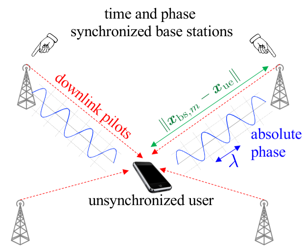
Figure 1: The received signal from each BS information contains information about the distance in both the ToA and the carrier phase. The BSs are time and phase synchronized, while the user is not.

CPP has been studied extensively in the context of global navigation satellite system (GNSS) positioning, via either precise point positioning (PPP) or real-time kinematic (RTK), relying on observations over time from several satellites [7]. Inherent to all CPP approaches is the so-called integer ambiguity, which refers to the fact that an observed phase is proportional to distance modulo the signal wavelength. The integer ambiguity renders both the positioning problem, as well as its analysis, more challenging. In the context of 5G, studies have considered both the integration with GNSS CPP [8] and 5G stand-alone CPP [6]. Focusing on the stand-alone operation, several studies have been conducted in recent years [9, 10, 11, 12, 13, 14, 6, 15, 16], considering both frequency range (FR) 1 (below 6 GHz) and to a lesser extent FR2 (mmWave, above 24 GHz). In [1], several practical challenges for CPP are identified, including the integer ambiguities and multipath, and new opportunities are highlighted, including novel pilots optimized for CPP. In FR1, [9, 10] demonstrated opportunistic 5G CPP for unmanned aerial vehicle (UAV) tracking, while the other studies focused on simulations. In particular, [11] shows how to perform carrier phase tracking for positioning with orthogonal frequency-division multiplexing (OFDM) signals from time and frequency synchronized BSs, considering aspects of multipath and phase wrapping, while [12] shows that CPP in FR1 provides sub-meter accuracies for both static and dynamic users. The use of reference stations, common in GNSS RTK, was also explored for 5G positioning [6, 15]. CPP has also been combined with various MIMO configurations, such as massive MIMO [16] for tracking phase information from multipath components, cell-free MIMO [13] for evaluating the impact of dense multipath, and near-field tracking [17]. In FR2, [14] uses CPP for inter-BS synchronization and user equipment (UE) tracking. An in-depth performance evaluation of CPP can be found in 3GPP report [18]. Surprisingly, despite this variety of algorithmic work, few papers have addressed the problem of fundamental performance bounds, which are useful for gaining deeper insights without the need for time-consuming simulations. While [19, 13, 17] conducted Cramér-Rao bound (CRB) analyses, neither considered the ambiguity. In [20], the ambiguity was considered, but only in a small range. In [17], the absolute phase was not utilized for positioning, so there was no ambiguity.

In this paper, we consider the CPP problem in its simplest form (i.e., snapshot positioning of an unsynchronized UE from ToA and carrier phase measurements from respect to several BSs, as shown in Fig. 1) in order to derive a novel fundamental performance bound. Our contributions are as follows: (i) We develop the signal model, revealing when the integer ambiguity appears in going from the waveform observation to the delay and phase observation; (ii) We derive a novel bound, the mixed-integer Cramér-Rao bound (MICRB), which accounts for the integer ambiguity; (iii) Via simulations, we demonstrate the tightness and usefulness of the bound, and show under which conditions CPP is most promising, including for cell-free MIMO systems.

II System Model

We consider a scenario with 1 UE, $M\geq 4$ BSs. The UE has an unknown position $\bm{x}_{\text{ue}}\in\mathbb{R}^{3}$ and is not synchronized to the BSs. We further assume that the BSs are all mutually phase synchronized and have known locations $\bm{x}_{\text{bs},m}\in\mathbb{R}^{3}$. In case the time or phase synchronization does not hold, a reference station (RS) can be used for computing differential measurements in which the per-BS time and phase biases are removed. For simplicity, we assume that any frequency offsets among all entities have been corrected.

OFDM pilot signals with unit-modulus pilots are transmitted by the BSs, comprising $N$ subcarriers with subcarrier spacing $\Delta_{f}$. The $M$ BSs transmit orthogonal OFDM waveforms (i.e., each BS uses $N/M$ different subcarriers per OFDM symbol and $M$ OFDM symbols) with a transmit power $P_{\text{tx}}$. After filtering, sampling, and cyclic prefix removal and combining over OFDM symbols, the frequency-domain signal (i.e., across the subcarriers) in terms of in-phase and quadrature (IQ) samples at the UE from BS $m$ under ideal line-of-sight (LoS) is given by [4, eq. (1)–(2)]

$$\bm{y}_{\text{iq},m}=\sqrt{E}_{s}\alpha_{m}\bm{d}(\tau_{m})+\bm{w}_{m},$$ (1)

where $E_{s}$ is the energy per subcarrier (with $E_{s}=P_{\text{tx}}/(N\Delta_{f})$), $\alpha_{m}=\rho_{m}e^{\jmath\vartheta_{m}}$ is the complex channel gain (in which $\rho_{m}\in\mathbb{R}$ captures the effect of path loss and transmitter and receiver antenna gains), $\tau_{m}$ is the ToA, $[\bm{d}(\tau)]_{n}=e^{-{\jmath 2\pi n\Delta_{f}\tau}}$ for $n\in\{0,\ldots,N-1\}-(N-1)/2$ is the centered delay steering vector, and $\bm{w}_{m}\sim\mathcal{CN}(\bm{0}_{N\times 1},N_{0}\bm{I}_{N\times N})$ is the noise. We also introduce $W=N\Delta_{f}$ as the system bandwidth. Under the stated assumptions, the ToA and carrier phase are related to the geometry by

$$\tau_{m} =\frac{1}{c}\|\bm{x}_{\text{bs},m}-\bm{x}_{\text{ue}}\|+B_{\text{ue}}$$ (2)

$$\vartheta_{m} =\frac{2\pi}{\lambda}\|\bm{x}_{\text{bs},m}-\bm{x}_{\text{ue}}\|+\phi_{\text{ue}},$$ (3)

where $B_{\text{ue}}$ is the clock bias of the UE, $\phi_{\text{ue}}$ is the phase bias of the UE. The objective of the UE is to estimate its position $\bm{x}_{\text{ue}}$ from $\bm{y}_{\text{iq},m}$, for $m=1,\ldots,M$.

III Observation Model and Performance Bounds

In this section, we first present an observation model of the ToA and carrier phase, from which we will derive the different bounds.

III-A Intermediate Observation Model

In order to derive all performance bounds, we will adopt a two-stage estimation process, where first the ToA and carrier phase are estimated from $\bm{y}_{\text{iq},m}$, as say $\hat{\tau}_{\text{ue},m}$ and $\hat{\vartheta}_{\text{ue},m}$, and then the UE position is determined. It is important to note that $\hat{\vartheta}_{\text{ue},m}$ is an estimate of $\phi_{\text{ue}}+{2\pi}\|\bm{x}_{\text{bs},m}-\bm{x}\|/\lambda$ modulo $2\pi$. Hence, we can express the ToA and phase observations directly as distances $y_{\tau,m}=\hat{\tau}_{\text{ue},m}\times c$ and $y_{\vartheta,m}=\hat{\vartheta}_{\text{ue},m}\times\lambda/(2\pi)$, given by

$$y_{\tau,m} =\|\bm{x}_{\text{bs},m}-\bm{x}_{\text{ue}}\|+B_{\text{ue}}c+w_{\tau,m}$$ (4)

$$y_{\vartheta,m} =\|\bm{x}_{\text{bs},m}-\bm{x}_{\text{ue}}\|+z_{m}\lambda+\phi_{\text{ue}}\frac{\lambda}{2\pi}+w_{\vartheta,m},$$ (5)

where $z_{m}\in\mathbb{Z}$ is unknown.

Stacking observations from different BSs, we introduce $\bm{y}=[\bm{y}^{\top}_{\tau}\bm{y}^{\top}_{\vartheta}]^{\top}$, where $\bm{y}_{\tau}=[y_{\tau,1},\ldots,y_{\tau,M}]^{\top}\in\mathbb{R}^{M}$ and $\bm{y}_{\vartheta}=[y_{\vartheta,1},\ldots,y_{\vartheta,M}]^{\top}\in\mathbb{R}^{M}$. Stacking the unknowns, we introduce $\bm{\eta}=[\bm{s}^{\top},\bm{z}^{\top}]^{\top}\in\mathbb{R}^{5}\times\mathbb{Z}^{M}$, where $\bm{s}=[\bm{x}^{\top}_{\text{ue}},B_{\text{ue}},\phi_{\text{ue}}]^{\top}$. As shown in the Appendix, the lower bounds on the error covariance matrices of the noises $\bm{w}_{\tau}$ and $\bm{w}_{\vartheta}$ are diagonal matrices $\bm{\Sigma}_{\tau}$ and $\bm{\Sigma}_{\vartheta}$, where $[\bm{\Sigma}_{\tau}]^{-1}_{m}={2\,\text{SNR}_{m}\pi^{2}W^{2}}/{(3c^{2})}$ and $[\bm{\Sigma}_{\vartheta}]^{-1}_{m}={8\,\text{SNR}_{m}\pi^{2}}/{\lambda^{2}}$, in which $\text{SNR}_{m}=NE_{s}\rho_{m}^{2}/N_{0}$.

III-B Classical Performance Bounds

From the observation model (4)–(5), classical performance bounds are derived, which ignore the integer ambiguities $\bm{z}$ [21], or relax the ambiguities to real numbers.

III-B1 Known Integer Ambiguity

When $\bm{z}$ is known, an optimistic bound is obtained. The Fisher information matrix (FIM) of $\bm{s}=[\bm{x}^{\top}_{\text{ue}},B_{\text{ue}},\phi_{\text{ue}}]^{\top}$ is given by

$$\bm{J}_{\text{known}}(\bm{s})$$ (6)

$$=\left[\begin{array}[]{ccc}\bm{U}\bm{J}\bm{U}^{\top}&c\bm{U}\text{diag}(\bm{J}_{\tau})&\frac{\lambda}{2\pi}\bm{U}\text{diag}(\bm{J}_{\vartheta})\\ c(\bm{U}\text{diag}(\bm{J}_{\tau}))^{\top}&\text{tr}(\bm{J}_{\tau})c^{2}&0\\ \frac{\lambda}{2\pi}(\bm{U}\text{diag}(\bm{J}_{\vartheta}))^{\top}&0&\text{tr}(\bm{J}_{\vartheta})\frac{\lambda^{2}}{(2\pi)^{2}}\end{array}\right],$$ (10)

where $\bm{J}_{\vartheta}=\bm{\Sigma}^{-1}_{\vartheta}$, $\bm{J}_{\tau}=\bm{\Sigma}^{-1}_{\tau}$, $\bm{J}=\bm{J}_{\vartheta}+\bm{J}_{\tau}$, and $\bm{U}=[\bm{u}_{1},\ldots,\bm{u}_{M}]$, in which $\bm{u}_{m}=(\bm{x}_{\text{ue}}-\bm{x}_{\text{bs},m})/\|\bm{x}_{\text{ue}}-\bm{x}_{\text{bs},m}\|$. By inverting $\bm{J}_{\text{known}}(\bm{s})$, the error covariance bound on the position is readily obtained, i.e., $\bm{\Sigma}_{\text{known}}(\bm{x}_{\text{ue}})=[\bm{J}^{-1}_{\text{known}}({\bm{s}})]_{1:3,1:3}$.

III-B2 Delay-only Bound

When the carrier phase observation $\bm{y}_{\vartheta}$ is not considered, the FIM of $\tilde{\bm{s}}=[\bm{x}^{\top}_{\text{ue}},B_{\text{ue}}]^{\top}$ is given by

$$\bm{J}_{\text{delay}}(\tilde{\bm{s}})= \left[\begin{array}[]{cc}\bm{U}\bm{J}_{\tau}\bm{U}^{\top}&c\bm{U}\text{diag}(\bm{J}_{\tau})\\ c(\bm{U}\text{diag}(\bm{J}_{\tau}))^{\top}&\text{tr}(\bm{J}_{\tau})c^{2}\end{array}\right].$$ (13)

After inversion and extraction of the first $3\times 3$ block, we obtain $\bm{\Sigma}_{\text{delay}}(\bm{x}_{\text{ue}})=[\bm{J}^{-1}_{\text{delay}}(\tilde{\bm{s}})]_{1:3,1:3}$.

III-B3 Floating Integer Ambiguity Bound

We consider $\bm{z}$ is an unconstrained real vector, so that in (5), $\phi_{\text{ue}}/{(2\pi)}$ is absorbed in each $z_{m}$. The estimate of $\bm{z}\in\mathbb{R}^{M}$ is known as the float solution. Hence, $\bm{\eta}$ becomes $\bm{\eta}=[\tilde{\bm{s}}^{\top},\bm{z}^{\top}]^{\top}\in\mathbb{R}^{4+M}$. After some manipulations of the FIM of $\bm{\eta}$, it can be shown that the bound on the error covariance of $\bm{z}\in\mathbb{R}^{M}$ is

$$\bm{\Sigma}_{\text{unc}}=\frac{1}{\lambda^{2}}\bm{\Sigma}_{\vartheta}+\frac{1}{\lambda^{2}}\bm{U}^{\top}\bm{\Sigma}_{\text{delay}}(\bm{x}_{\text{ue}})\bm{U},$$ (14)

while the bound on the error covariance on $\tilde{\bm{s}}$ is the same as in the delay-only case.

III-C Proposed Mixed-Integer Bound

We first express the stacked observation as

$$\bm{y} =\tilde{\bm{f}}(\tilde{\bm{s}})+\bm{B}\bm{z}+\kappa\bm{B}\bm{1}_{M\times 1}+\bm{w},$$ (15)

where $\bm{z}\in\mathbb{Z}^{M}$, $\bm{w}\sim\mathcal{N}(\mathbf{0}_{2M},\bm{\Sigma}_{\text{ch}})$, $\bm{\Sigma}_{\text{ch}}=\text{blkdiag}(\bm{\Sigma}_{\tau},\bm{\Sigma}_{\vartheta})$, $\bm{f}(\cdot)$ is a nonlinear function of $\tilde{\bm{s}}$, defined as, for $m=1,\ldots,M$,

$$[\tilde{\bm{f}}(\tilde{\bm{s}})]_{m} =\|\bm{x}_{\text{bs},m}-\bm{x}_{\text{ue}}\|+B_{\text{ue}}c$$ (16)

$$[\tilde{\bm{f}}(\tilde{\bm{s}})]_{M+m} =\|\bm{x}_{\text{bs},m}-\bm{x}_{\text{ue}}\|.$$ (17)

In addition, $\bm{B}=[\bm{0}_{M\times M};\lambda\bm{I}_{M\times M}]\in\mathbb{R}^{2M\times M}$, and $\kappa=\phi_{\text{ue}}/(2\pi)$. Note that $\kappa$ and $\bm{z}$ are not jointly identifiable. To address this, we will reduce the state dimension. In particular, we express

$$\bm{y}=\tilde{\bm{f}}(\tilde{\bm{s}})+\bm{B}\left[\begin{array}[]{c}0\\ \bm{D}\bm{z}\end{array}\right]+\kappa_{\text{d}}\bm{B}\bm{1}_{M\times 1}+\bm{w},$$ (20)

where $\bm{D}=[-\bm{1}_{(M-1)\times 1}\,\bm{I}_{(M-1)\times(M-1)}]$ and $\kappa_{\text{d}}=\kappa+z_{1}$, in which $z_{1}$ is the first entry of $\bm{z}.$ From this, we introduce $\bm{z}_{\text{d}}\doteq\bm{D}\bm{z}\in\mathbb{Z}^{M-1}$. Then we can write

$$\bm{y}=\bm{f}({\bm{s}})+\bm{B}\bm{E}\bm{z}_{\text{d}}+\bm{w},$$ (21)

where $\bm{f}({\bm{s}})=\tilde{\bm{f}}(\tilde{\bm{s}})+\kappa_{\text{d}}\bm{B}\bm{1}_{M\times 1}$ and $\bm{E}=[\bm{0}^{\top}_{(M-1)\times 1};\bm{I}_{(M-1)\times(M-1)}]$.

From the identifiable formulation (21), we proceed with the following steps: (i) Considering $\bm{z}\in\mathbb{R}^{M}$, we obtain the floating integer ambiguity bound $\bm{\Sigma}_{\text{unc}}$ on $\bm{z}$ and the bound $\bm{\Sigma}_{\text{delay}}(\bm{x}_{\text{ue}})$ on $\bm{x}_{\text{ue}}$. (ii) We determine the probability of making specific errors $\bm{\delta}\in\mathbb{Z}^{M-1}$ when determining the integer solution $\bm{z}_{\text{d}}$ from the float solution. (iii) An integer ambiguity error in $\bm{z}_{\text{d}}$ leads to a biased estimate of $\bm{s}$. This bias will be characterized. (iv) We put everything together to compute the final error covariance on $\bm{s}$, considering the integer ambiguity errors, their biases, and their probabilities.

III-C1 Integer Ambiguity Errors

We decompose the float solution $\hat{\bm{z}}_{\text{unc}}\in\mathbb{R}^{M}$ into

$$\hat{\bm{z}}_{\text{unc}}=\bm{E}\bm{z}_{\text{d}}+\kappa_{\text{d}}\bm{1}_{M\times 1}+\bm{u},\bm{u}\sim\mathcal{N}(\bm{0},\bm{\Sigma}_{\text{unc}}).$$ (22)

We next determine a differential observation

$$\bm{D}\hat{\bm{z}}_{\text{unc}} =\bm{D}\bm{E}\bm{z}_{\text{d}}+\kappa_{\text{d}}\bm{D}\bm{1}_{M\times 1}+\bm{D}\bm{u}$$ (23)

$$=\bm{z}_{\text{d}}+\bm{D}\bm{u}$$ (24)

since $\bm{D}\bm{1}_{M\times 1}=\bm{0}_{(M-1)\times 1}$. We whiten the noise, leading to an observation $\bm{r}=\bm{S}^{-1/2}\bm{z}_{\text{d}}+\mathbf{u}^{\prime}$, where $\bm{r}=\bm{S}^{-1/2}\bm{D}\hat{\bm{z}}_{\text{unc}}$, $\mathbf{u}^{\prime}\sim\mathcal{N}(\bm{0}_{(M-1)\times 1},\bm{I}_{(M-1)\times(M-1)})$ and $\bm{S}=\bm{D}\bm{\Sigma}_{\text{unc}}\bm{D}^{\top}$. Finally, we recover $\bm{z}_{\text{d}}$ by solving the following integer problem

$$\hat{\bm{z}}_{\text{d}}=\arg\min_{\bm{z}_{\text{d}}\in\mathbb{Z}^{M-1}}\|\bm{r}-\bm{S}^{-1/2}\bm{z}_{\text{d}}\|,$$ (25)

which can be solved efficiently with standard toolboxes [22], provided $M$ is not too large. From $\hat{\bm{z}}_{\text{d}}$, we introduce the integer error $\bm{\delta}=\hat{\bm{z}}_{\text{d}}-\bm{z}_{\text{d}}$.

III-C2 Bias in $\bm{s}$ due to Integer Ambiguity Error

To determine the bias in ${\bm{s}}$, we linearize (21) around ${\bm{s}}$. With a slight abuse of notation, this leads to $\bm{y}=\bm{A}{\bm{s}}+\bm{B}\bm{E}\bm{z}_{\text{d}}+\bm{w}$, after removing irrelevant terms, and in which $\bm{A}=\nabla_{{\bm{s}}}\bm{f}({\bm{s}})\in\mathbb{R}^{2M\times 5}$, computed at the true value of $\bm{s}$. After whitening the noise and computing the least-squares estimate of ${\bm{s}}$, the bias is immediately recovered as

$$\bm{b}({\bm{s}}|\bm{\delta})=(\bm{\Sigma}^{-1/2}_{\text{ch}}\bm{A})^{\dagger}\bm{\Sigma}^{-1/2}_{\text{ch}}\bm{B}\bm{E}\bm{\delta},$$ (26)

where $\bm{X}^{\dagger}$ is the Moore-Penrose inverse of the tall matrix $\bm{X}$, i.e., $\bm{X}^{\dagger}=(\bm{X}^{\top}\bm{X})^{-1}\bm{X}^{\top}$.

III-C3 Mixed Integer CRB

To now computed the MICRB, we first recall that when the estimator of $\tilde{\bm{s}}$ is biased with bias $\bm{b}({\bm{s}}|\bm{\delta})$, the resulting error covariance is (including the bias) [23]

$$\bm{\Sigma}({\bm{s}}|\bm{\delta})=\bm{b}({\bm{s}}|\bm{\delta})(\bm{b}({\bm{s}}|\bm{\delta}))^{\top}+(\bm{I}+\bm{H}_{\bm{b}})\bm{\Sigma}_{\text{known}}({\bm{s}})(\bm{I}+\bm{H}_{\bm{b}})^{\top}$$ (27)

where $\bm{H}_{\bm{b}}=\nabla_{{\bm{s}}}\bm{b}({\bm{s}}|\bm{\delta})\in\mathbb{R}^{5\times 5}$. Finally, the proposed bound on the error covariance is obtained by taking the expectation with respect to the integer ambiguity error:

$$\bm{\Sigma}_{\text{mi}}({\bm{s}}) =\sum_{\bm{\delta}\in\mathbb{Z}^{M-1}}\text{Pr}(\bm{\delta})\bm{\Sigma}({\bm{s}}|\bm{\delta}).$$ (28)

The summation can be efficiently computed via Monte Carlo simulation. To do this, we generate $N_{s}$ samples $\bm{r}^{(i)}=\bm{S}^{-1/2}\bm{z}_{\text{d}}+\bm{u}^{(i)}$, where ${\bm{u}}^{(i)}\sim\mathcal{N}(\bm{0}_{M-1},\bm{I}_{M-1})$ and determine the estimate $\hat{\bm{z}}_{\text{d}}^{(i)}$. From this, we obtain ${\bm{\delta}}^{(i)}=\hat{\bm{z}}_{\text{d}}^{(i)}-\bm{z}_{\text{d}}$. Finally, $\bm{\Sigma}_{\text{mi}}({\bm{s}})\approx{1}/{N_{s}}\sum_{i=1}^{N_{s}}\bm{\Sigma}({\bm{s}}|\bm{\delta}^{(i)})$.

III-C4 Complexity Analysis

Due to the involved sampling (with complexity scaling linearly in $N_{s}$) and the need to solve (25) for each sample (with complexity scaling at least cubically in $M$ [24]), the complexity of the proposed MICRB is far higher than the conventional counterparts from Section III-B.

IV Positioning Algorithms

In this section, we describe two distinct approaches to solve the CPP problem: the first one is based directly on (21), while the second one is based on directional statistics. These algorithms are not the main contributions of this work and are presented to provide a baseline for the bounds.

IV-A Mixed Integer Approach

The maximum likelihood (ML) problem can be expressed as

$$\hat{\bm{s}},\hat{\bm{z}}_{\text{d}}=\arg\min_{\bm{s}\in\mathbb{R}^{5},\bm{z_{\text{d}}}\in\mathbb{Z}^{M-1}}\|\bar{\bm{y}}-\bm{\Sigma}^{-1/2}_{\text{ch}}\bm{f}(\bm{s})-\bar{\mathbf{B}}\bm{z}_{\text{d}}\|^{2}.$$ (29)

where $\bar{\bm{y}}=\bm{\Sigma}^{-1/2}_{\text{ch}}\bm{y}$ and $\bar{\mathbf{B}}=\bm{\Sigma}^{-1/2}_{\text{ch}}\bm{B}\bm{E}$. Solving this problem is challenging, due to the combination of the nonlinearity $\bm{f}(\cdot)$ and the integer variable $\bm{z}_{\text{d}}$. To deal with this, the standard solution involves several steps [25]. First, we linearize (21) around some value ${\bm{s}}_{0}$:

$$\bm{y}\approx\bm{f}({\bm{s}}_{0})+\nabla\bm{f}({\bm{s}}_{0})\delta{\bm{s}}+\bm{B}\bm{E}\bm{z}_{\text{d}}+\bm{w},$$ (30)

where we recall that ${\bm{s}}=[\bm{x}^{\top}_{\text{ue}},B_{\text{ue}},\phi_{\text{ue}}]^{\top}$. To obtain ${\bm{s}}_{0}$, we solve

$$\min_{\bm{x}_{\text{ue}},B_{\text{ue}}}\sum_{m=1}^{M}\frac{\left(y_{\tau,m}-\|\bm{x}_{\text{bs},m}-\bm{x}_{\text{ue}}\|-cB_{\text{ue}}\right)^{2}}{2\sigma^{2}_{\tau,m}}$$ (31)

using any conventional time-difference-of-arrival (TDoA) method. This provides ${\bm{s}}_{0}$, in which we set $\hat{\phi}_{\text{ue}}=0$ since it appears linearly. Then, after removing $\bm{f}({\bm{s}}_{0})$, we are left with

$$\bm{y}^{\prime}=\nabla\bm{f}({\bm{s}}_{0})\delta{\bm{s}}+\bm{B}\bm{E}\bm{z}_{\text{d}}+\bm{w}.$$ (32)

We can then find an unconstrained estimate of $\bm{z}_{\text{d}}$ and then solve (25) to obtain the integer estimate of $\bm{z}_{\text{d}}$. Finally, we obtain a closed-form solution of $\delta\bm{s}$ from (32), considering $\bm{z}_{\text{d}}$ to be known.

IV-B Directional Statistics Approach

As an alternative approach, we can avoid integer ambiguities by working with directional statistics, where we model the carrier phase measurements with a von Mises distribution [26]. Then, the negative log-likelihood function (LLF) becomes

$$-\log p(\bm{y}|\bm{x}_{\text{ue}},B_{\text{ue}},\phi_{\text{ue}})=$$ (33)

$$\sum_{m=1}^{M}\frac{\left(y_{\tau,m}-\|\bm{x}_{\text{bs},m}-\bm{x}_{\text{ue}}\|-cB_{\text{ue}}\right)^{2}}{2\sigma^{2}_{\tau,m}}+$$

$$\sum_{m=1}^{M}\frac{\lambda^{2}}{(2\pi)^{2}\sigma^{2}_{\vartheta,m}}{\cos\Big{(}\Big{(}\frac{2\pi}{\lambda}y_{\vartheta,m}-\frac{2\pi}{\lambda}\|\bm{x}_{\text{bs},m}-\bm{x}_{\text{ue}}\|\Big{)}-\phi_{\text{ue}}\Big{)}}.$$

To solve (33), we note that for a given $\bm{x}_{\text{ue}}$, we can easily determine $B_{\text{ue}}$ (in closed form) and $\phi_{\text{ue}}$ (by a 1D search). The method thus proceeds as follows. From the ToA measurements, a coarse estimate of $\bm{x}_{\text{ue}}$ is obtained, as in (31). Then, a fine grid around $\bm{x}_{\text{ue}}$ is defined with step size dependent on the bound $\bm{\Sigma}_{\text{known}}(\bm{x}_{\text{ue}})$ and a grid size dependent on the bound $\bm{\Sigma}_{\text{delay}}(\bm{x}_{\text{ue}})$. For each trial location, $B_{\text{ue}}$ and $\phi_{\text{ue}}$ are determined and the solution with minimal negative log-likelihood is selected. Overall, this method requires a fine 4D search, which is computationally complex.

V Numerical Results

V-A Scenario

We consider a UE at a fixed location $\bm{x}_{\text{ue}}=[0;0;5]^{\top}$ and $M$ BSs located in 3D space, with $\bm{x}_{\text{bs},m}\sim\mathcal{N}(\bm{0},(0.1~{}\text{km})^{2}\bm{I}_{3\times 3})$. The default system parameters are as follows: carrier frequency $f_{c}=28~{}\text{GHz}$, subcarrier spacing $\Delta_{f}=20~{}\text{kHz}$, $N=300$ subcarriers, $-174~{}\text{dBm/Hz}$ noise power spectral density, a receiver noise figure of $13~{}\text{dB}$, transmission power of $0~{}\text{dBm}$, and $M=7$ BSs. We set $\rho_{m}=\lambda/(4\pi\|\bm{x}_{\text{bs},m}-\bm{x}_{\text{ue}}\|)$, to model the dependence of the free space path loss on the carrier frequency.

V-B Bounds and Algorithms

Performance of algorithms will be measured in terms of the root mean squared error (RMSE), while the bounds will be represented by the position error bound (PEB), defined as $\text{PEB}=\sqrt{\text{trace}(\bm{\Sigma}(\bm{x}_{\text{ue}}))}$. The RMSE and PEB are both expressed in meters. We will study the following bounds: the bound with known integer ambiguity based on (6), the delay-only bound from (13), and the proposed MICRB (28) computed with $N_{s}=1000$. We will present the following algorithms: the mixed integer approach from Section IV-A, the directional statistics approach from Section IV-B, and the delay-only estimator.

V-C Results and Discussion

We will evaluate the impact of the following parameters: the carrier frequency, the bandwidth, the transmission power, and the number of BSs. When varying one parameter, the other parameters are set to their default values.

V-C1 Impact of Carrier Frequency

Figure 2: Impact of carrier frequency on PEB and positioning RMSE.

Figure 3: LLF at 3 GHz carrier for delay only and combined delay and carrier phase observations.

Figure 4: LLF at 30 GHz carrier for delay only and combined delay and carrier phase observations.

Figure 5: Impact of bandwidth on PEB and positioning RMSE.

We first vary the carrier frequency $f_{c}$, leading to the results in Fig. 2. This figure reveals several interesting facts. The PEB for delay-only estimation ($\text{PEB}_{\text{delay}}$) increases with carrier frequency, due to the increasing path loss. In contrast, the PEB with known ambiguity ($\text{PEB}_{\text{known}}$) is relatively constant, due to two counter-acting effects: large path loss (leading to lower SNR) vs. smaller wavelength (leading to better carrier phase estimates for a given SNR). The proposed bound $\text{PEB}_{\text{mi}}$ has a markedly different behavior: for low carrier frequencies (below 20 GHz) it coincides with $\text{PEB}_{\text{known}}$, while for higher carrier frequencies (above 50 GHz), it coincides with $\text{PEB}_{\text{delay}}$. The reason for this will be discussed shortly. Focusing on the algorithms, we observe that both methods show a similar trend as $\text{PEB}_{\text{mi}}$, with the mixed-integer approach performing worse for carriers below 30 GHz, while the directional statistics approach deviates from the bound above 30 GHz. To understand the transitions, we consider a 1D cut of the LLF at 3 GHz (Fig. 3) and at 30 GHz (Fig. 4). At 3 GHz the wavelength (10 cm) is on the order of the uncertainty of the delay-only position estimates. This means that the LLF near the delay-only estimate is relatively smooth. Since the SNR is high enough, there is a clear peak around the true value, separate from the peak of the delay-only LLF. At 30 GHz, the delay-only LLF is much broader (due to the increased path loss), while phase estimates in units of cycles also become worse due to path loss, which means that although the carrier phase accuracy in meter units does not degrade, this accuracy becomes actually worse with respect to the wavelength. the wavelength has become much smaller. The overall effect on the combined LLF is shown. Note that there are many local optima, with LLF close to the global optimum. This leads to an increased probability of selecting the wrong optimum, corresponding to an integer ambiguity error.

V-C2 Impact of Bandwidth

In this section, we vary the bandwidth, as shown in Fig. 5. We observe that $\text{PEB}_{\text{delay}}$ improves with bandwidth, as expected, while $\text{PEB}_{\text{known}}$ is approximately constant since the quality of the carrier phase estimates is independent of the bandwidth. The proposed MICRB has a different behavior: for small bandwidths, we have poor delay estimation, leading again to a similar effect as shown in Fig. 4, so that the bound coincides with the $\text{PEB}_{\text{delay}}$. As the bandwidth increases, the delay estimates get better, while the carrier phase estimates maintain the same quality. Combined, the MICRB improves. After a bandwidth of 300 MHz (when the delay estimation is on the order to 10 $\lambda$), the MICRB touches $\text{PEB}_{\text{known}}$, as this case is similar to Fig. 3. Fig. 2 and Fig. 5 combined clearly show that carrier phase positioning is possible with any bandwidth and any carrier frequency, but not with any arbitrary combination of both. In summary, the bandwidth must be sufficiently large so that the delay estimates are good enough with respect to the wavelength.

Figure 6: Impact of transmission power on PEB and positioning RMSE.

Figure 7: Impact of number of BSs on PEB and positioning RMSE.

V-C3 Impact of Transmission Power

When we instead change the transmission power (see Fig. 6), a different story emerges. Both $\text{PEB}_{\text{delay}}$ and $\text{PEB}_{\text{known}}$ improve with transmission power (due to increased SNR) and lead to roughly parallel curves. The proposed MICRB has a thresholding behavior, where for sufficiently large transmit power, a more pronounced global optimum of the carrier phase estimate leads us to correctly identify the correct optimum. We see that the directional statistic approach (33) closely follows the MICRB, while the mixed integer approach (29) is unable to improve upon the delay-only estimator. This effect can be ascribed to the poor delay estimates for all considered transmit powers so that the linearization point $\bm{s}_{0}$ used in (30) is far away from the ML solution. These results clearly indicate that the mixed integer approach requires a good delay-only estimate, while the directional statistics approach does not.

V-C4 Impact of Number of BSs

As a last result, we vary the number of BSs (see Fig. 7). In this figure, BSs are progressively added when computing the bound $\text{PEB}_{\text{delay}}$ and $\text{PEB}_{\text{known}}$ tend to be relatively flat since performance is dominated by a few BSs with good geometry and SNR. In correspondence to the results as a function of transmission power, we can predict that the mixed-integer algorithm will fail to attain $\text{PEB}_{\text{known}}$, due to poor delay estimates, for the considered number of BSs. The directional statistics approach does not suffer from this shortcoming and closely follows the MICRB $\text{PEB}_{\text{mi}}$, harnessing the unique global optimum of the NLL. This shows the great promise of positioning using for instance cell-free deployments, where each UE will be surrounded by many phase-coherent access points [13].

VI Conclusions

This paper studied the CPP problem in a cellular context, considering a snapshot positioning scenario under LoS conditions. A new fundamental performance bound is derived that can account for the inherent integer ambiguity of the CPP positioning problem. The new bound is demonstrated to be tighter than previously known bounds, at a cost of higher complexity. Results as a function of carrier frequency, bandwidth, transmission power, and the number of BSs reveal surprising insights as to when carrier phase information can be harnessed. In particular, the standard mixed-integer approach may be far from optimal when the delay estimates are poor. There are several possible extensions of this work, including (i) the presence of multipath, (ii) a blocked LoS path; (iii) reducing the complexity of the MICRB.

References

- [1] J. Nikonowicz et al., “Indoor Positioning Trends in 5G-Advanced: Challenges and Solution towards Centimeter-level Accuracy,” Dec. 2022, arXiv:2209.01183 [cs, math].
- [2] T. Wild et al., “Joint design of communication and sensing for beyond 5G and 6G systems,” IEEE Access, vol. 9, pp. 30 845–30 857, 2021.
- [3] A. Behravan et al., “Positioning and sensing in 6G: Gaps, challenges, and opportunities,” IEEE Vehicular Technology Magazine, 2022.
- [4] H. Wymeersch et al., “Radio localization and sensing—Part I: Fundamentals,” IEEE Communications Letters, vol. 26, no. 12, pp. 2816–2820, 2022.
- [5] J. A. del Peral-Rosado et al., “Survey of cellular mobile radio localization methods: From 1G to 5G,” IEEE Communications Surveys & Tutorials, vol. 20, no. 2, pp. 1124–1148, 2017.
- [6] A. Fouda et al., “Toward cm-level accuracy: Carrier phase positioning for IIoT in 5G-Advanced NR networks,” in IEEE PIMRC, Kyoto, Japan, Sep. 2022, pp. 782–787.
- [7] P. Teunissen et al., “Review and principles of PPP-RTK methods,” Journal of Geodesy, vol. 89, no. 3, pp. 217–240, 2015.
- [8] P. Zheng et al., “5G-aided RTK positioning in GNSS-deprived environments,” arXiv preprint arXiv:2303.13067, 2023.
- [9] J. Khalife et al., “Opportunistic UAV navigation with carrier phase measurements from asynchronous cellular signals,” IEEE Transactions on Aerospace and Electronic Systems, vol. 56, no. 4, pp. 3285–3301, 2019.
- [10] A. A. Abdallah et al., “UAV navigation with 5G carrier phase measurements,” in Proceedings of the 34th International Technical Meeting of the Satellite Division of The Institute of Navigation, 2021, pp. 3294–3306.
- [11] H. Dun et al., “Positioning in a multipath channel using OFDM signals with carrier phase tracking,” IEEE Access, vol. 8, pp. 13 011–13 028, 2020.
- [12] L. Chen et al., “Carrier phase ranging for indoor positioning with 5G NR signals,” IEEE Internet of Things Journal, 2021.
- [13] A. Fascista et al., “Uplink joint positioning and synchronization in cell-free deployments with radio stripes,” IEEE International Conference on Communications (ICC) Workshops, 2023.
- [14] S. Fan et al., “Carrier phase-based synchronization and high-accuracy positioning in 5G new radio cellular networks,” IEEE Transactions on Communications, vol. 70, no. 1, pp. 564–577, 2021.
- [15] J. Li et al., “Carrier Phase Positioning Using 5G NR Signals Based on OFDM System,” in IEEE VTC, London, United Kingdom, 2022.
- [16] X. Li et al., “Massive MIMO-Based Localization and Mapping Exploiting Phase Information of Multipath Components,” IEEE Transactions on Wireless Communications, vol. 18, no. 9, pp. 4254–4267, Sep. 2019.
- [17] A. Guerra et al., “Near-field tracking with large antenna arrays: Fundamental limits and practical algorithms,” IEEE Trans. Signal Process., vol. 69, pp. 5723–5738, Aug. 2021.
- [18] 3GPP, Study on expanded and improved NR positioning (Release 18), March 2022.
- [19] N. Vukmirović et al., “Performance limits of direct wideband coherent 3d localization in distributed massive mimo systems,” Sensors, vol. 21, no. 10, p. 3401, 2021.
- [20] D. Medina et al., “Cramér-Rao bound for a mixture of real- and integer-valued parameter vectors and its application to the linear regression model,” Signal Processing, vol. 179, p. 107792, 2021.
- [21] H. L. Van Trees, Detection, estimation, and modulation theory, part I: detection, estimation, and linear modulation theory. John Wiley & Sons, 2004.
- [22] X.-W. Chang et al., “Miles: Matlab package for solving mixed integer least squares problems, version 2.0,” 2011.
- [23] Y. C. Eldar, “Uniformly improving the Cramér-Rao bound and maximum-likelihood estimation,” IEEE Transactions on Signal Processing, vol. 54, no. 8, pp. 2943–2956, 2006.
- [24] B. Hassibi et al., “On the sphere-decoding algorithm i. expected complexity,” IEEE transactions on signal processing, vol. 53, no. 8, pp. 2806–2818, 2005.
- [25] Z. Wang et al., “A new method of integer parameter estimation in linear models with applications to GNSS high precision positioning,” IEEE Transactions on Signal Processing, vol. 69, pp. 4567–4579, 2021.
- [26] J. Cai et al., “The statistical property of the GNSS carrier phase observations and its effects on the hypothesis testing of the related estimators,” in ION GNSS, 2007, pp. 331–338.