A Poincaré covariant cascade method for high-energy nuclear collisions

Abstract

We present a Poincaré covariant cascade algorithm based on the constrained Hamiltonian dynamics in an $8N$-dimensional phase space to simulate the Boltzmann-type two-body collision term. We compare this covariant cascade algorithm with traditional $6N$-dimensional phase-space cascade algorithms. To validate the covariant cascade algorithm, we perform box calculations. We examine the frame dependence of the algorithm in a one-dimensionally expanding system as well as the compression stages of colliding two nuclei. We confirm that our covariant cascade method is reliable to simulate high-energy nuclear collisions. Furthermore, we present Lorentz-covariant equations of motion for the $N$-body system interacting via potentials, which can be efficiently solved numerically.

I Introduction

High-energy heavy-ion collisions offer a unique opportunity to study hot and dense nuclear matter Luo et al. (2022); Sorensen et al. (2023). To extract equilibrium properties of nuclear matter, such as equations of state, it is necessary to describe the dynamics of finite and non-equilibrium systems using a theoretical transport approach. Transport models have been widely used in the past few decades to understand collision dynamics and experimental data in high-energy heavy-ion collisions. These models include parton cascade models Geiger (1997); Zhang (1998); Molnar and Gyulassy (2000); Xu and Greiner (2005); Lin et al. (2005), Boltzmann-Uhlenbeck-Uehling (BUU) models Bertsch and Das Gupta (1988), and quantum molecular dynamics (QMD) approaches Aichelin (1991), as well as their relativistic extensions Buss et al. (2012); Sorge et al. (1989); Maruyama et al. (1991). Extensive comparisons of various transport models can be found in Refs. Xu et al. (2016); Zhang et al. (2018); Ono et al. (2019); Colonna et al. (2021); Wolter et al. (2022).

One of the main ingredients of non-equilibrium microscopic transport approaches is a Boltzmann-type collision term, which is often simulated by the so-called cascade method, e.g., a scattering happens when the closest distance between two particles is less than the interaction range given by the cross section $d=\sqrt{\sigma/\pi}$, where $\sigma$ is the total cross section. However, this geometrical interpretation of cross section often leads to a violation of Lorentz covariance for the $N$ interacting particle system in the $6N$-dimensional phase-space approach. To address this issue, numerical codes employ effective algorithms to approximate the relativistic effect in the modeling. Despite the lack of covariance in these transport models, reasonable results are obtained when a simulation is performed in the global center-of-mass frame of colliding two nuclei. It is important to note that different collision algorithms lead to different numerical results Zhang and Pang (1997); Cheng et al. (2002); Zhang et al. (2018); Ono et al. (2019); Zhao et al. (2020). The causality problems in the cascade models were discussed in Refs. Kodama et al. (1984); Kortemeyer et al. (1995); Zhang and Pang (1997); Zhang et al. (1998); Xu and Greiner (2005); Zhao et al. (2020). The full-ensemble (subdivision) method Welke et al. (1989); Lang et al. (1993); Zhang et al. (1998); Molnar and Gyulassy (2000) can reduce the causality violation, but it alters event-by-event corrections and fluctuations and is computationally expensive.

A Poincaré covariant Hamiltonian formalism for an $N$-interacting particle system can be constructed based on the framework of constrained Hamiltonian dynamics Sudarshan et al. (1981); Samuel (1982a, b) by extending the phase space from the non-relativistic $6N$ to $8N$ dimensions to avoid the no-interaction theorem Currie (1963); Currie et al. (1963); Leutwyler (1965), where four-positions and four-momenta of particles are the dynamical variables. The framework of constrained Hamiltonian dynamics Sudarshan et al. (1981); Samuel (1982a, b) was utilized to develop a relativistic version of quantum molecular dynamics (RQMD) Sorge et al. (1989); Maruyama et al. (1991, 1996); Isse et al. (2005); Mancusi et al. (2009); Marty and Aichelin (2013) to describe the dynamics of interacting particles by mean-field potentials. New versions of RQMD approaches are developed later by implementing Lorentz-vector potentials Nara and Stoecker (2019); Nara et al. (2020); Nara and Ohnishi (2022).

In this paper, we propose a Poincaré covariant cascade method based on the framework of constrained Hamiltonian dynamics Sudarshan et al. (1981); Samuel (1982a, b). This method allows efficient numerical simulations of the collision processes in $8N$-dimensional phase space, which is as efficient as the standard cascade method in a $6N$-dimensional phase space. In the constrained Hamiltonian dynamics, the $N$-particle system is described in terms of $8N$-dimensional phase space. To ensure that the dynamical system has the physical degrees of freedom of $6N$, we impose $2N$ constraints. We employ the same constraints as in Refs. Maruyama et al. (1996); Mancusi et al. (2009); Marty and Aichelin (2013); Nara and Stoecker (2019); Nara et al. (2020); Nara and Ohnishi (2022), which were shown to describe interacting $N$ relativistic particles effectively through potentials. We compare our approach with other models that employ different constraints Sorge et al. (1989); Maruyama et al. (1991) to investigate the difference and advantages of our proposed method. Our covariant cascade method has been implemented in the event generator JAM Nara et al. (2000); Nara (2019) to simulate high-energy nuclear collisions for a wide range of beam energy.

This paper is organized as follows: In Sec. II, we summarize cascade methods in the $6N$-dimensional phase space. In Sec. III, a Poincaré covariant cascade method in $8N$-dimensional phase space will be presented. Section IV is dedicated to the comparison and validation of different collision schemes. We examine the collision rate and thermal spectra in a box calculation. To investigate frame dependence, we first analyze a one-dimensionally expanding system considering only elastic scatterings. Then, different collision schemes are applied to collisions of two nuclei in different computational frames, including inelastic processes. We also evaluate various collision schemes in the $6N$-dimensional phase space Zhang (1998); Bass et al. (1998); Zhao et al. (2020). Our analysis reveals that some of the collision schemes provide a reasonable description of the collision term when applied in the center-of-mass system under specific conditions. In Sec. V, we will introduce new covariant equations of motion for a $N$-particle system interacting through potentials, which is numerically efficient. The conclusion is given in Sec. VI. Throughout this paper, we use the natural unit system of $c=k_{B}=1$ and the sign convention of the metric $g_{\mu\nu}=\operatorname{diag}(+,-,-,-)$.

II Cascade methods in $6N$-dimensional phase space

We first summarize several cascade algorithms in the $6N$-dimensional phase space. In these cascade models, the geometrical interpretation of the cross section is commonly employed, where two particles will collide if the impact parameter $b$ becomes smaller than the interaction range specified by the cross section $\sigma$: $b\leq\sqrt{\sigma/\pi}$. The impact parameter is defined as the minimum distance in the two-body center-of-mass system (c.m.s.). Let us consider the collision of two particles with coordinates, $q_{1}=(t_{1},\bm{x}_{1})$ and $q_{2}=(t_{2},\bm{x}_{2})$, and momenta, $p_{1}=(E_{1},\bm{p}_{1})$ and $p_{2}=(E_{2},\bm{p}_{2})$. The Lorentz invariant expression of the squared impact parameter is given by Kodama et al. (1984); Sasaki (2001); Hirano and Nara (2012)

$$b^{2}=\bm{x}_{\mathrm{cm}}^{2}-\frac{(\bm{x}_{\mathrm{cm}}\cdot\bm{v}_{\mathrm{cm}})^{2}}{\bm{v}_{\mathrm{cm}}^{2}}=-q_{T}^{2}+\frac{(q\cdot p_{T})^{2}}{p_{T}^{2}},$$ (1)

where $\bm{x}_{\mathrm{cm}}=\bm{x}_{\mathrm{cm},1}-\bm{x}_{\mathrm{cm},2}$ is the relative position between the two particles, and $\bm{v}_{\mathrm{cm}}=\bm{v}_{\mathrm{cm},1}-\bm{v}_{\mathrm{cm},2}$ is the relative velocity in the two-body c.m.s., respectively. The four-vectors $q_{T}$ and $p_{T}$ are the transverse relative position and momentum,

$$q =q_{1}-q_{2}, p =p_{1}-p_{2},$$ (2)

$$q_{T} =q-(q\cdot u)u, p_{T} =p-(p\cdot u)u,$$ (3)

where $u$ is the unit vector proportional to the total momentum of the two-body system

$$u=\frac{p_{1}+p_{2}}{\sqrt{(p_{1}+p_{2})^{2}}}.$$ (4)

The time of the closest approach, $t_{\mathrm{cm}}$, in the two-body c.m.s.,

$$t_{\mathrm{cm}} =t_{\mathrm{cm},1}+\lambda(p_{1},p_{2},+q)(p_{1}\cdot u),$$ (5)

$$t_{\mathrm{cm}} =t_{\mathrm{cm},2}+\lambda(p_{2},p_{1},-q)(p_{2}\cdot u),$$ (6)

is Lorentz invariant quantities, where $t_{\mathrm{cm},1}$ and $t_{\mathrm{cm},2}$ denotes the last collision times of the respective particles in the two-body c.m.s., and

$$\lambda(p_{1},p_{2},q)=\frac{p_{2}^{2}(q\cdot p_{1})-(p_{1}\cdot p_{2})(q\cdot p_{2})}{(p_{1}p_{2})^{2}-p_{1}^{2}p_{2}^{2}}.$$ (7)

The times of the closest approach $t_{c1}$ and $t_{c2}$ for the two colliding particles in the computational frame are obtained by Lorentz transforming $t_{cm}$ (see Appendix A):

$$\begin{split}t_{c1}&=t_{1}+\lambda(p_{1},p_{2},+q)E_{1},\\ t_{c2}&=t_{2}+\lambda(p_{2},p_{1},-q)E_{2}.\end{split}$$ (8)

Although the times of the closest approach are simultaneous in the two-body c.m.s., they are, in general, different in a computational frame, which can lead to the violation of causality. The two particles may collide when their impact parameter is less than the interaction range $\sqrt{\sigma/\pi}$ and $t_{c1}>t_{1}$ and $t_{c2}>t_{2}$ to avoid backward collision in time. We make a collision list by ordering all possible collision pairs. The collision list is updated after every collision. Thus, we need to define the collision ordering time Zhang and Pang (1997); Zhao et al. (2020). The ordering time, $t_{o}$, is used to order the collisions in the collision list to determine which particle pair collides first in the time-step–free cascade calculation. The collision times, $t_{\mathrm{coll1}}$ and $t_{\mathrm{coll2}}$, are the times at which the two particles collide, i.e., change their momentum (and species in inelastic scattering), which may be different from the time of closest approach.

There is no unambiguous guideline to specify the ordering time. The ZPC parton cascade model assumes the ordering time to be the average of the times of the closest approach: $t_{o}=(t_{c1}+t_{c2})/2$, and assumes that the collision times are the same as the ordering time $t_{\mathrm{coll1}}=t_{\mathrm{coll2}}=t_{o}$. This approach is referred to as collision scheme G (CS-G) in Ref. Zhao et al. (2020). Another possible choice is to define the ordering time to be the minimum of the times of the closest approach: $t_{o}=\min(t_{c1},t_{c2})$, which predicts a less collision rate Xu and Greiner (2005) (collision scheme A (CS-A)) with the collision times being the same as the times of the closest approach: $t_{\mathrm{coll1}}=t_{c1}$ and $t_{\mathrm{coll2}}=t_{c2}$. In Ref. Zhao et al. (2020), a collision scheme, in which the collision times and the collision ordering time are chosen by the minimum: $t_{\mathrm{coll1}}=t_{\mathrm{coll2}}=t_{o}=\min(t_{c1},t_{c2})$ (collision scheme B (CS-B)), accurately describes the collision rate and the equilibrium momentum distribution in a box calculation. The distinct difference in the collision schemes is that two particles collide simultaneously in their two-body c.m.s. in CS-A, while in CS-B and CS-G, the collision time of two colliding particles is the same in the computational frame.

There are problems in these schemes due to the different times for the closest approach in the computational frame. For example, in collision scheme CS-A, the particle with a larger collision time would not collide in the duration between the collision times $|t_{c1}-t_{c2}|$ to avoid non-causal collisions, which reduces the collision rate Zhang et al. (1998). We note that particles do not collide at the distance of the closest approach in collision schemes CS-B and CS-G. In these collision schemes, to avoid non-causal collisions, we impose the additional conditions: $t_{\mathrm{coll1}}>t_{1}$ and $t_{\mathrm{coll2}}>t_{2}$.

As an alternative approach, the proper time interval $\delta\tau_{i}(j)$ from the last collision time $\tau_{i}$ to the next collision time $\tau_{ci}(j)$ for the collision of particles $i$ with particle $j$ at the closest approach

$$\delta\tau_{i}(j) =\tau_{ci}(j)-\tau_{i}=\lambda(p_{i},p_{j},q_{i}-q_{j})\sqrt{p_{i}^{2}},$$ (9)

are considered for the ordering of two-body collisions in Ref. Kodama et al. (1984). It is argued that in this approach, if only causal collisions are required, the number of collisions is largely reduced and may lead to the underestimation of the collision rate Kortemeyer et al. (1995).

To avoid the problems of collision ordering, one can introduce the time step, and collision pairs are randomly selected by using the predicted collision times in Eq. (8)  Wolf et al. (1990). We note that the Lorentz transformation of Eq. (9) to the computational frame yields Eq. (8). In this approach, a sufficiently small time-step size should be selected to avoid the artifact of the order of the collision and decay sequence Ono et al. (2019). In addition, the comparisons of $N(N-1)/2$ pairs in a $N$-particle system have to be made at each time step, which leads to the increasing computational time proportional to $N^{2}$.

In UrQMD Bass et al. (1998) and SMASH Weil et al. (2016), the collision ordering time and the collision time are defined as the time of the closest approach in the computational reference frame,

$$t_{\mathrm{coll}}^{\mathrm{(ref)}}=t_{1}-\frac{[\bm{x}_{1}(t_{1})-\bm{x}_{2}(t_{1})]\cdot(\bm{v}_{1}-\bm{v}_{2})}{(\bm{v}_{1}-\bm{v}_{2})^{2}},$$ (10)

where coordinates and velocities $\bm{v}_{1}$ and $\bm{v}_{2}$ are taken in the computational frame. It should be noted that the impact parameter is still defined in the two-body c.m.s. frame. Let us call the collision scheme with this collision ordering CS-O. This collision scheme does not have problems arising from the difference in collision times.

As one possible way to recover the Lorentz covariance, the full-ensemble method has been proposed Welke et al. (1989); Lang et al. (1993); Zhang et al. (1998); Molnar and Gyulassy (2000), in which particles are over-sampled by the factor of $N_{\mathrm{test}}$: $n\to nN_{\mathrm{test}}$ and the cross section is reduced by $\sigma\to\sigma/N_{\mathrm{test}}$. As the density $\rho$ scales as $N_{\mathrm{test}}$, the mean free path remains the same $\ell\sim(\rho\sigma)^{-1}$. Since the collision distance scales as $d=\sqrt{\sigma/\pi}\propto 1/\sqrt{N_{\mathrm{test}}}$, the collision occurs at the same space-time point in the limit of $N_{\mathrm{test}}\to\infty$ so that the collision term of the Boltzmann equation is recovered. However, this method destroys the event-by-event fluctuations and correlations. Furthermore, it requires intensive computational time.

As an alternative method, the “local-ensemble method” Danielewicz and Bertsch (1991); Lang et al. (1993); Cassing (2002), which is also called the “stochastic method” Xu and Greiner (2005) was developed based on the covariant collision rate. We first divide the space into a set of small volumes and introduce over-sampled test particles by the factor $N_{\mathrm{test}}$. When the number of collisions occurring in volume $dV$ in a time interval $dt$ is given by Landau and Lifschits (1975)

$$d\nu =\sigma v_{M}n_{1}n_{2}dVdt, v_{M} =\frac{\sqrt{(p_{1}\cdot p_{2})^{2}-p_{1}^{2}p_{2}^{2}}}{p_{1}^{0}p_{2}^{0}},$$ (11)

one obtains the collision probability in volume $dN$ and time interval $dt$ as

$$P_{22}=\frac{d\nu}{dN_{1}dN_{2}}=\frac{\sigma}{N_{\mathrm{test}}}v_{M}\frac{dt}{dV},$$ (12)

where $n_{i}=dN_{i}/dV$. In each time step, the collision pairs are randomly chosen from the volume. In the limits of $dV\to 0$, $dt\to 0$, and $N_{\mathrm{test}}\to\infty$, the collision rate converges to the exact solutions of the Boltzmann equation. This approach has the advantage that multi-particle collisions such as $m\to n$ processes can be simulated in a straightforward way Cassing (2002); Staudenmaier et al. (2021); Coci et al. (2023). The stochastic method generally requires a large number of test particles to ensure the accurate solution of the Boltzmann equation. The cell length should be smaller than the mean free path to reduce numerical artifacts. This method was first used to solve the BUU transport model, which solves the time evolution of the one-particle phase space function.

III Poincaré Covariant cascade models

We now consider the Poincaré covariant cascade method in the $8N$-dimensional phase space in terms of four-vectors of the particle positions and momenta to construct a covariant cascade method.

III.1 Covariant cascade method from the constrained Hamiltonian formalism

According to Dirac’s constrained Hamiltonian formalism, the Hamiltonian is given by a linear combination of $2N-1$ constraints,

$$H=\sum_{i=1}^{2N-1}u_{i}\phi_{i}.$$ (13)

The trajectories of four-positions $q_{i}(\tau)$ and four-momenta $p_{i}(\tau)$ are parametrized by the Poincaré invariant evolution parameter $\tau$. The equations of motion are given by

$$\frac{dq^{\mu}_{i}}{d\tau} = [H,q_{i}^{\mu}]=\sum_{j=1}^{2N-1}u_{j}\frac{\partial\phi_{j}}{\partial p_{i\mu}},$$ (14)

$$\frac{dp^{\mu}_{i}}{d\tau} = [H,p_{i}^{\mu}]=-\sum_{j=1}^{2N-1}u_{j}\frac{\partial\phi_{j}}{\partial q_{i\mu}},$$ (15)

where the Poisson brackets are defined as

$$[A,B]=\sum_{k}\left(\frac{\partial A}{\partial p_{k}}\cdot\frac{\partial B}{\partial q_{k}}-\frac{\partial A}{\partial q_{k}}\cdot\frac{\partial B}{\partial p_{k}}\right).$$ (16)

In the cascade method, particles travel on the straight-line trajectory as if they are free most of the time, and the collision takes place at discrete points in $\tau$. Thus, we take the following mass-shell constraints:

$$H_{i}=\phi_{i}=p_{i}^{2}-m_{i}^{2},\quad i=1,\ldots,N\,.$$ (17)

The remaining $N$ constraints, which we call time fixation, fix the times of particles. Different time fixations will be discussed in the following subsections.

The Lagrange multipliers $u_{i}$ are determined by requiring the invariance of the constraints during the time evolution:

$$\frac{d\phi_{i}}{d\tau}=[H,\phi_{i}]+\frac{\partial\phi_{i}}{\partial\tau}=\sum_{j=1}^{2N-1}C_{ij}u_{j}+\frac{\partial\phi_{i}}{\partial\tau}=0,$$ (18)

where $C_{ij}=[\phi_{j},\phi_{i}]$. Since the mass shell constraints commute $[H_{i},H_{j}]=0$, the Lagrange multipliers can be obtained by solving $N\times N$ system of linear equations for $u_{j}$.

In the following, we will discuss different realizations of cascade models within the constrained Hamiltonian formulation by employing different time fixations.

III.2 Sorge’s constraints

One of the main requirements in relativistic particle dynamics is the cluster separability. The cluster separability means that when the Minkowski distance between two clusters of particles is space-like and sufficiently large, they do not interact with each other.

Based on the idea Samuel (1982b), Sorge proposed the following time constraints Sorge et al. (1989), which satisfy the cluster separability,

$$\chi_{i}=\sum_{i\neq j}G_{ij}u_{ij}\cdot q_{ij}=0,\quad i=1,\ldots,N-1,$$ (19)

where $p_{ij}=p_{i}+p_{j}$, $q_{ij}=q_{i}-q_{j}$, and $u_{ij}=p_{ij}/\sqrt{p_{ij}^{2}}$. The evolution parameter $\tau$ may be fixed by the gauging condition Maruyama et al. (1991) that equates the average time of particles in the global c.m.s. to $\tau$:

$$\chi_{N}=Q\cdot U-\tau=0,$$ (20)

where

$$Q =\frac{1}{N}\sum_{i=1}^{N}q_{i}, P =\sum_{i}p_{i}, U =\frac{P}{\sqrt{P^{2}}}.$$ (21)

The weight function $G_{ij}$ only depends on the Minkowski distance $q_{ij}$ and is chosen as

$$G_{ij}=\frac{\exp\left(q_{ij}^{2}/L\right)}{q_{ij}^{2}/L},$$ (22)

where we use $L=8$ fm². In these constraints, the times of the interacting two particles in their c.m.s. are equal in the dilute limit. The terms $1/q_{ij}^{2}$ are introduced to keep the space-like distance between two particles to maintain the causality.

Numerical implementation of the constraints (19) is quite challenging for the simulation of realistic collisions. At every two-body collision and decay, time constraints (19) break. Thus, one needs to solve the non-linear equations in $N$ unknowns to recover the time constraints after every collision or decay. It is too time-consuming to perform such numerical simulations on a current computer. In addition, the standard Newton-Raphson method often does not find the solution. Therefore, we simulate an approximate solution of the constraints by introducing time steps, and we try to recover the time constraints at every time step. We recognize clusters at every time step and solve these constraints for each cluster. Furthermore, we approximate the solution in only one iteration in the Newton-Raphson method. We also assume that the Lagrange multiplier $u_{i}$ remains the same during each time step after two-body collisions. It should be mentioned that in the actual numerical simulations, the constraints given by Eq. (19) occasionally result in a negative Lagrange multiplier $u_{i}$, which means that the $i$th particle moves backward in time. In such cases, we assume that the Lagrange multiplier is equal to zero, $u_{i}=0$.

III.3 Poincaré covariant parton cascade model

The Poincaré covariant parton cascade (PCPC)  Borchers et al. (2000) is an alternative approach for a manifestly covariant formulation of the cascade model. This model is based on a Hamiltonian formulation that allows $N$ particles to move freely in an $8N$-dimensional phase space. The Hamiltonian for the free particle system Peter et al. (1994); Behrens et al. (1994) is given by

$$H=\sum_{i=1}^{N}\frac{p_{i}^{2}-m_{i}^{2}}{2m_{i}},$$ (23)

and Hamilton’s equations of motion specify the world lines of particles

$$\frac{dq_{i}}{d\tau}=\frac{p_{i}}{m_{i}}\equiv u_{i},$$ (24)

where the four-position vector $q_{i}$ is a function of the Poincaré invariant parameter $\tau$. In the case of a massless particle system, the Hamiltonian Kurkela et al. (2022)

$$H=\sum_{i=1}^{N}\frac{\lambda}{2}p_{i}^{2}$$ (25)

gives the equations of motion

$$\frac{dq_{i}}{d\tau}=\lambda p_{i},$$ (26)

where $\lambda$ is an arbitrary constant. The collision can happen when the two-body distance in the center-of-mass system becomes the closest.

Let us consider this approach based on the constrained Hamiltonian dynamics. The first $N$ constraints are the same as the free mass-shell constraints. To find the time constraints, by multiplying $u_{i}$ by both sides of Eq. (24), one obtains

$$u_{i}\cdot\frac{dq_{i}}{d\tau}=1.$$ (27)

After integrating Eq. (27) over $\tau$, the time fixation constraints are expected to be

$$\chi_{i} = u_{i}\cdot[q_{i}(\tau)-q_{i}(\tau_{0i})]-\tau+\tau_{0i},$$ (28)

where $i$ runs over $i=1,\ldots,N$. Indeed, the Lagrange multipliers are given by $u_{i}=1/(2p_{i}\cdot u_{i})=1/2m_{i}$ and we obtain the equations of motion (24). One can choose the initial coordinate $q_{i}(\tau_{0i})$ and evolution parameter $\tau_{0i}$ for the particle arbitrarily at the collision point, thus there are no constraints in Eq. (28). Moreover, the time constraints do not depend on other particles.

Similarly, for the massless particle case, Eq. (26) implies

$$p_{i}\cdot\frac{dq_{i}}{d\tau}=0,\quad i=1,\ldots,N.$$ (29)

Thus, the equations of motion for massless particles may be obtained from the constraints

$$\phi_{i} =p_{i}^{2},\quad i=1,\ldots,N,$$ (30)

$$\phi_{N+i} =p_{i}\cdot[q_{i}(\tau)-q_{i}(\tau_{0i})],\quad i=1,\ldots,N-1,$$ (31)

$$\phi_{2N} =Q\cdot\frac{P}{P^{2}}-\lambda\tau,$$ (32)

where $Q=\sum_{i=1}^{N}q_{i}$ and $P=\sum_{i=1}^{N}p_{i}$. The last constraint implies $t_{\mathrm{cm}}=\lambda E_{\mathrm{cm}}\tau$, where $t_{\mathrm{cm}}=Q^{0}$ and $E_{\mathrm{cm}}=P^{0}$ in the global c.m.s. One finds that the Lagrange multipliers are the same for all particles: $u_{i}=\lambda/2$, and the equations of motion are identical to Eq. (26).

In the PCPC approach, the times of the particles elapse in proportion to their energies, and there is no time relation between particles. Times of the particles are randomly spread at later times. Consequently, particle distances can be time-like, which violates the causality because a particle can collide with an absolute-future particle. In a box simulation, ignoring such acausal collisions leads to a significant reduction in collision rate at late times. However, when simulating the collision of two nuclei, these effects may not be as relevant at a certain level because the momenta, and thus the times of particles are similar when they are close to each other in the coordinate space.

III.4 A new covariant cascade method

In this section, we introduce our covariant cascade method based on the constrained Hamiltonian dynamics taking the constraints used in Refs. Sudarshan et al. (1981); Maruyama et al. (1996) for the potential interactions. Specifically, we apply the mass shell constraints (17) and the following time constraints to formulate a cascade method for the first time:

$$\phi_{N+i} = \chi_{i}=\hat{a}\cdot(q_{i}-q_{N}),\quad i=1,\ldots,N-1,$$ (33)

$$\phi_{2N} = \chi_{N}=\hat{a}\cdot q_{N}-\tau,$$ (34)

where $\hat{a}$ is a Lorentz vector, which acts as a timekeeper. In Refs. Samuel (1982a); Marty and Aichelin (2013), $\hat{a}$ is defined as $\hat{a}^{\mu}=P^{\mu}/(P_{\mu}P^{\mu})^{1/2}$, where $P^{\mu}$ is the total momentum of the system. This choice equates the times of all particles in the global c.m.s. In other words, the evolution parameter $\tau$ is interpreted as the time as measured in the global c.m.s. Another way to specify $\hat{a}$ is to introduce a freely moving dummy particle and to specify $\hat{a}$ using the momentum of the dummy particle Sudarshan et al. (1981). If we choose the rest frame of the dummy particle as the global c.m.s., the two models become identical. We note that a different choice of timekeeper yields a different physical system of interacting particles. Throughout this work, we define $\hat{a}=(1,0,0,0)$ in the global c.m.s. We should note that the four-vector $\hat{a}$ is subject to the Poincaré transformation in switching to another computational frame so that the Poincaré covariance of the model is maintained.

The Lagrange multipliers are solved to be $u_{i}=1/(2\hat{a}\cdot p_{i})$, and the equations of motion are obtained as

$$\frac{dq_{i}}{d\tau}=\frac{p_{i}}{\hat{a}\cdot p_{i}}.$$ (35)

Note that $\hat{a}\cdot p_{i}$ is the energy of the $i$th particle in the frame in which $\hat{a}=(1,0,0,0)$. The time coordinate of the $i$th particle is identical to the evolution parameter $q_{i}^{0}=\tau$ in this frame, but it is different in other frames. We note that the physical velocity of the particle

$$\frac{d\bm{q}_{i}}{dq_{i}^{0}}=\frac{d\bm{q}_{i}}{d\tau}\frac{d\tau}{dq_{i}^{0}}=\frac{\bm{p}_{i}}{p_{i}^{0}}$$ (36)

is kept to be less than the speed of light.

Our approach satisfies the cluster separability in the sense that independent clusters do not interact with each other since the timekeeper $\hat{a}$ is a constant vector after specifying the computational frame. However, when a cluster is separated into clusters, the c.m.s. of each cluster is different from the original frame. This implies that to be consistent with the simulations started from the separated state as an initial condition, the different $\hat{a}$ must be reassigned to each cluster, which is not included in our constraints. We will discuss this issue with a different model in Sec. IV.4.

III.5 Closest distance approach in $8N$-dimensional phase space

Let us now consider a covariant cascade procedure. The main interest is to determine the collision point of two particles in a covariant way. This is straightforward in the $8N$-dimensional phase-space approach. In the cascade model, particles move in straight lines and change their momentum only by collisions or decays. The distance squared between two particles is defined as the distance in the two-body c.m.s.:

$$d^{2}=-q^{2}+\frac{(q\cdot P)^{2}}{P^{2}},$$ (37)

where $q=q_{1}-q_{2}$ and $P=p_{1}+p_{2}$. The time of the closest distance may be obtained by the condition

$$-\frac{1}{2}\frac{\partial d^{2}}{\partial\tau}=q_{T}\cdot v=q\cdot v_{T}=0,$$ (38)

where $v=\frac{dq}{d\tau}$ is the relative velocity, and

$$v_{T}=v-\frac{(v\cdot P)}{P^{2}}P$$ (39)

is the transverse relative velocity of the colliding two particles. Applying the closest distance condition $q\cdot v_{T}=0$ to the equations of motion of two particles,

$$q_{i}(\tau)=q_{i}(\tau_{i})+v_{i}\,(\tau-\tau_{i}),\quad i=1,2,$$ (40)

where $v_{i}=p_{i}/(\hat{a}\cdot p_{i})$ is a constant velocity in our model, we get the time of the closest approach $\tau_{\mathrm{coll}}$ as

$$\tau_{\mathrm{coll}}-\tau_{i} =-\frac{(q_{1}(\tau_{i})-q_{2}(\tau_{i}))\cdot v_{T}}{v_{T}^{2}},\quad i=1,2.$$ (41)

The two-body collision will occur at $\tau_{\mathrm{coll}}$, and it is ordered in $\tau$ in a frame-independent way. In this way, we avoid the frame dependence of the ordering time.

The closest distance $b^{2}$, i.e., squared impact parameter, may be obtained by

$$b^{2}=-q_{\mathrm{c}}^{2}+\frac{(q_{\mathrm{c}}\cdot P)^{2}}{P^{2}},$$ (42)

where $q_{\mathrm{c}}=q_{1}(\tau_{\mathrm{coll}})-q_{2}(\tau_{\mathrm{coll}})$ is the relative distance when the collision takes place. We note that $b^{2}$ is identical to the previously presented impact parameter (1) (see Appendix B).

IV Results

In the following, we validate the thermal distribution and collision rate of our covariant scheme within a box simulation assuming massless particles and elastic scattering. We compare the simulation results with analytical expressions. Next, we examine the frame dependence of the results for a one-dimensionally expanding system. Furthermore, we present simulation results of nucleus-nucleus collisions from compression stages to expansion stages, including inelastic processes.

In Table 1, we summarize the collision schemes that will be compared in this section.

Table 1: Different collision schemes in the closest approach. In the covariant collision scheme, collisions happen at a single collision time specified by the Lorentz invariant evolution parameter $\tau_{\mathrm{coll}}$. In CS-A, CS-B, and CS-G, the times of the closest approach for the two colliding particles are computed in the two-body center-of-mass system (c.m.s.), then these times are transformed to the computational frame, which is represented by $t_{c1}$ and $t_{c2}$. In CS-O, the collision time $t_{\mathrm{coll}}^{\mathrm{(ref)}}$ is the time of the closest approach computed in the computational frame. The frame where the impact parameter $b$ is defined is listed. Other collision schemes are examined in Ref. Zhao et al. (2020). We list CS-M in Ref. Zhao et al. (2020) to avoid confusion with CS-O.

	collision time	ordering time	frame of $b$
Covariant	$\tau_{\mathrm{coll}}$	$\tau_{\mathrm{coll}}$	two-body c.m.s
CS-A	$t_{c1}$ and $t_{c2}$	$\min(t_{c1},t_{c2})$	two-body c.m.s.
CS-B	$\min(t_{c1}$, $t_{c2})$	$\min(t_{c1},t_{c2})$	two-body c.m.s.
CS-G	$(t_{c1}$ + $t_{c2})/2$	$(t_{c1}+t_{c2})/2$	two-body c.m.s.
CS-O	$t_{\mathrm{coll}}^{\mathrm{(ref)}}$	$t_{\mathrm{coll}}^{\mathrm{(ref)}}$	two-body c.m.s.
CS-M	$t_{\mathrm{coll}}^{\mathrm{(ref)}}$	$t_{\mathrm{coll}}^{\mathrm{(ref)}}$	computational frame

IV.1 Box calculations

We first examine energy distribution in a box calculation. We assume massless gluons, elastic collisions with the cross section of $\sigma=2.6$ fm, and isotropic scattering Zhao et al. (2020). The coordinates of the particles are uniformly distributed, and the momenta of the particles are initialized as

$$\frac{dN}{Ndp_{T}dp_{z}}=\delta(p_{T}-1.5\,\mathrm{GeV})\delta(p_{z})$$ (43)

with the total number of particles $N=5400$ in the box size of 6 fm$\times$6 fm$\times$6 fm. At late times, the distribution should obey the Boltzmann form

$$\frac{dN}{NE^{2}dE}=\frac{1}{2T^{3}}e^{-E/T}.$$ (44)

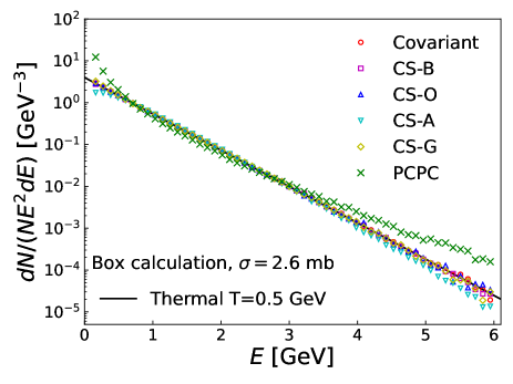
Figure 1: Energy distributions are compared for different collision schemes. The size of the box is 6 fm$\times$6 fm$\times$6 fm. The cross section for the massless gluons is set to 2.6 mb, and an isotropic angular distribution is assumed. The line represents the thermal distribution of temperature $T=0.5$ GeV.

Figure 1 compares the final energy distributions among different collision schemes in a box calculation together with the theoretical curve (44) with the temperature $T=0.5$ GeV. The final energy distributions are obtained after the global time of 5 fm/$c$. The energy distribution from collision scheme CS-G, which uses the average collision time for the ordering time, deviates from the thermal distribution. The results from the other collision schemes are in good agreement with the expected thermal distribution except for the PCPC approach. As explained in the previous section, the PCPC evolution does not have any time correlation between particles; particle times spread without any restriction, which leads to timelike distances between particles. This might be the main reason for unphysical distribution from the PCPC approach. We note that the results of the $6N$-dimensional phase-space cascade schemes of CS-B and CS-G are consistent with the results in Ref. Zhao et al. (2020).

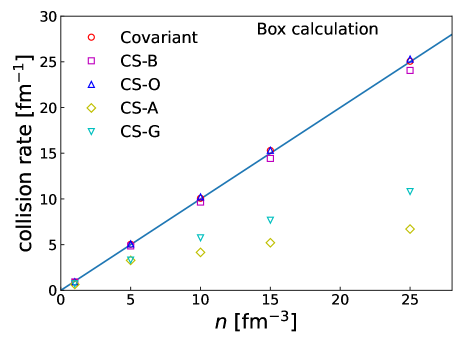
Figure 2: Collision rate per collision pair as a function of density. The size of the box is 6 fm$\times$6 fm$\times$6 fm. The cross section for the massless gluons is set to 10 mb, and an isotropic angular distribution is assumed. The line corresponds to the analytical expectation $\sigma n$.

In Fig. 2, the collision rates per collision pair in a box calculation are plotted as functions of density $n$ for different collision schemes. We use the cross section of $\sigma=10$ mb and isotropic scattering. Collision schemes CS-A and CS-G predict much lower collision rates than the analytical expectation $\sigma n$, which is consistent with the result in Refs. Xu and Greiner (2005); Zhao et al. (2020); the collision rate is significantly suppressed in schemes CS-A and CS-G when the mean free path is smaller than the interaction range because the number of non-causal collisions increases Zhang et al. (1998). The other collision schemes are consistent with the analytical expectation, including our covariant cascade method. As discussed in detail in Ref. Xu and Greiner (2005), the difference in the collision times in the computational frame in collision schemes CS-A and CS-G leads to the lower collision rate. Let us consider the collision of particles 1 and 2 with $t_{1}$ and $t_{2}$ being the times when the last collision of particles 1 and 2 happened. The times of the closest approach are denoted by $t_{c1}$ and $t_{c2}$. In the scheme CS-A, the collision ordering time is defined as the smaller one of the two collision times: $t_{o}=\min(t_{c1},t_{c2})$. In the situation $t_{1}<t_{c1}<t_{2}<t_{c2}$, the collision between particles 1 and 2 occurs at $t=t_{c1}$, which is earlier than $t_{2}$, the time of the collision between particle 2 and another. To forbid such non-causal collisions, we need an additional condition $t_{o}>t_{i},~{}i=1,2$, which reduces the number of collisions since possible collisions of particle 2 during the time interval $|t_{c1}-t_{c2}|$ are not considered. In contrast, collision scheme CS-B assumes the collision time and the ordering time to be the smallest one: $t_{o}=t_{\mathrm{coll1}}=t_{\mathrm{coll2}}=\min(t_{c1},t_{c2})$, which does not suppress possible collisions in the interval $|t_{c1}-t_{c2}|$. The collision rate in the collision scheme CS-B is close to the analytical one in the box simulation as found in Ref. Zhao et al. (2020). The collision scheme CS-O, in which the collision times of particles and the collision ordering time are the same and are determined in the computational frame, correctly reproduces the analytical value since there is no problem arising from the difference in the collision times.

IV.2 One-dimensionally expanding systems

To study the frame dependence of cascade results, we examine a one-dimensionally expanding system that is motivated by the initial conditions at RHIC (Relativistic Heavy Ion Collider). For this purpose, we adopt the same initial condition as in Ref. Zhang and Pang (1997). Specifically, we consider a system consisting of $N=4000$ gluons that are uniformly distributed within a spacetime rapidity interval $\eta\in[-5,5]$. The transverse distribution of particles is assumed to be a disk of radius 5 fm. The momentum distribution of the particles is taken from the Boltzmann distribution with the temperature of 0.5 GeV and boosted with the velocity $\beta=\tanh\eta_{i}$, where $\eta_{i}$ is the spacetime rapidity of the $i$th particle. The times and longitudinal positions of particles are then obtained, assuming the formation time of $\tau_{0}=0.1$ fm/c,

$$t_{i} =\tau_{0}\cosh\eta_{i}, z_{i} =\tau_{0}\sinh\eta_{i}.$$ (45)

The transverse positions $\bm{x}_{Ti}$ are propagated up to the formation time, $\bm{x}_{Ti}(t_{i})=\bm{x}_{Ti}(0)+\bm{v}_{Ti}t_{i}$. To study the frame dependence, we boost the above initial condition defined in the global c.m.s. (the collider frame) using the velocity $\beta=\tanh\eta_{0}$ with $\eta_{0}=5$ (the target frame).

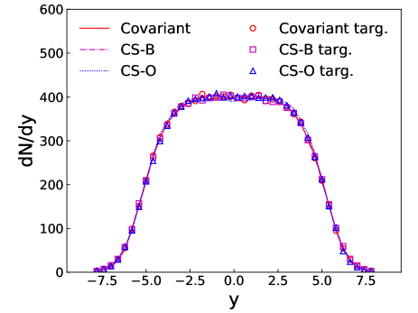
Figure 3: Rapidity distributions are compared for different collision schemes. The cross section for the massless gluons is set to 3.5 mb, and an isotropic angular distribution is assumed. The solid, dashed-dotted, and dotted lines correspond to the results from the covariant collision scheme, CS-B, and CS-O in the collider frame. The results from the target frame are shown by the circles, squares, and triangles for the covariant collision scheme, CS-B, and CS-O, respectively.

In Fig. 3, we compare the rapidity distributions with different collision schemes for different frames. The solid, dashed-dotted, and dotted lines correspond to the results from the covariant cascade, CS-B, and CS-O, respectively. The corresponding results from the calculations in the target frame are expressed by symbols. We do not show collision schemes CS-A and CS-G because the frame dependencies turned out to be the same as that of scheme CS-B. In the one-dimensionally expanding system with elastic collisions, we do not see frame dependence even for the non-covariant collision schemes. In Ref. Zhang and Pang (1997), strong frame dependence is observed in the collision scheme in which both the collision frame and the defining frame of the impact parameter of the two-body scattering are the computational frame. In collision scheme CS-O, the time of the closest approach is computed in the computational frame while the impact parameter is defined in the two-body c.m.s. frame of colliding pair. This is the reason why the frame dependence is greatly suppressed in collision scheme CS-O.

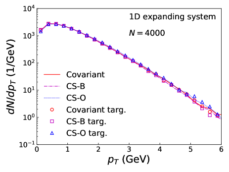
Figure 4: Transverse momentum distributions are compared for different collision schemes The cross section for the massless gluons is set to 3.5 mb, and an isotropic angular distribution is assumed. The meaning of the lines and symbols is the same as in Fig. 3.

The transverse momentum distributions are compared in Fig. 4. The results from three collision schemes in the collider frame are indistinguishable. We see a slight enhancement of the transverse energy in collision scheme CS-O in the target frame.

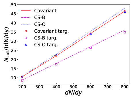
Figure 5: The total number of collisions normalized by the $dN/dy$ as a function of $dN/dy$ for the one-dimensionally expanding initial condition. The cross section for the massless gluons is set to 3.5 mb, and an isotropic angular distribution is assumed. The meaning of the lines and symbols are the same as in Fig. 3.

In Fig. 5, we compare the $dN/dy$ dependence of the total number of collisions per $dN/dy$. We consider three collision schemes: covariant, CS-B, and CS-O (see more details in the previous section). While these schemes exhibit similar behavior in the box calculation, they show noticeable differences in the expanding system. The covariant collision scheme predicts the same number of collisions for both the collider frame and the target frame as it should, while the number of collisions in the target frame is slightly smaller in the non-covariant collision schemes, CS-B and CS-O. This suppression of collision number in the target frame is also reported in Ref. Zhang and Pang (1997). The number of collisions in CS-B becomes very small compared to the covariant scheme in the expanding system, contrary to the static box calculations. Collision scheme CS-O predicts a slightly larger collision number than the covariant scheme in the collider frame, although the difference between the covariant scheme and CS-O is very small. Let us consider a collision of two particles with $t_{1}$ and $t_{2}$ (assuming $t_{1}<t_{2}$ without loss of generality) where the times of the closest approach are given by $t_{c1}$ and $t_{c2}$. In collision scheme CS-B, the collision time is assumed to be the minimum of the times of the closest approach. As discussed in the previous section, CS-B requires the condition $t_{c1}>t_{2}$ to prevent non-causal collisions. The times of all particles are different in the initial condition (45) unlike the box initial conditions, where the initial times of all particles are set to zero. This expanding initial condition might be a part of the reasons for the reduction of the collision number in CS-B. A possible reason for the slight enhancement of the collision number in CS-O may be due to the effects of the flow because CS-O computes the time of the closest approach in the computational frame, while the others compute in the two-body c.m.s.

IV.3 AA and pA collisions

In the preceding section, we examined different collision schemes for a one-dimensionally expanding system assuming only elastic scatterings. In this section, we extend our investigation to include other effects such as particle production, decay, and the compression stages of nuclear collisions, which involve more violent reactions compared to the expanding stages. For this purpose, we examine the central Au + Au (Pb + Pb) and p + Au collisions using the event generator JAM Nara et al. (2000); Nara (2019), in which particle productions are modeled by the excitations of resonances and strings, followed by their decays. The nuclear collisions are simulated from the compression stages to the expanding stages, covering the entire collision process until all the particles freeze out.

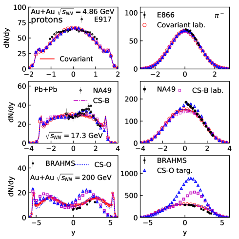
Figure 6: Rapidity distributions of protons and negative pions in central Au + Au collisions at $\sqrt{s_{NN}}=4.86$ GeV (upper panels) $\sqrt{s_{NN}}=200$ GeV (lower panels), and central Pb + Pb collision at $\sqrt{s_{NN}}=17.3$ GeV (middle panels) are compared with different collision schemes. The solid, dashed-dotted, and dotted lines correspond to the results of the calculations from the covariant collision scheme, CS-B, and CS-O in the center-of-mass frame. The results of calculations in the target frame are presented by circles, squares, and triangles in the covariant collision scheme, CS-B, and CS-O, respectively. Experimental data were taken from Back et al. (2002); Ahle et al. (1998); Anticic et al. (2011); Appelshauser et al. (1999); Afanasiev et al. (2002); Bearden et al. (2004, 2005).

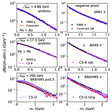
Figure 7: Transverse mass distributions of protons and negative pions in central Au + Au collision at $\sqrt{s_{NN}}=4.86$ GeV (upper panels), in central Pb + Pb collision at $\sqrt{s_{NN}}=17.3$ GeV (middle panels), and in central Au + Au collision at $\sqrt{s_{NN}}=200$ GeV (lower panels). The BRAHMS proton data are divided by factor 2 to correct weak decay contribution roughly. The meaning of the lines and symbols are the same as in Fig. 6. Experimental data were taken from Ahle et al. (1998); Alt et al. (2006); Afanasiev et al. (2002); Bearden et al. (2004, 2005).

Figures 6 and 7 show the rapidity and transverse mass distributions of protons and negative pions in central Au + Au collisions at $\sqrt{s_{NN}}=4.86$ GeV (upper panels), $\sqrt{s_{NN}}=200$ GeV (lower panels), and central Pb + Pb collisions at $\sqrt{s_{NN}}=17.3$ GeV (middle panels) calculated by the JAM2 cascade mode with different collision schemes. The impact parameter $b\leq 3.4$ fm is chosen to approximately simulate the 5% central collisions. The three different collision schemes, covariant, CS-B, and CS-O, are compared including the frame dependence. The three collision schemes yield almost identical rapidity and transverse mass distributions for protons and pions for all three beam energies when simulating in the global c.m.s. However, a weak frame dependence is observed for the collision at $\sqrt{s_{NN}}=4.86$ GeV. The frame dependence becomes more pronounced at $\sqrt{s_{NN}}=17.3$ GeV and even stronger at $\sqrt{s_{NN}}=200$ GeV. The frame dependence of scheme CS-O turned out to be more significant compared with scheme CS-B.

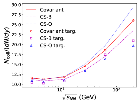
Figure 8: Collision energy dependence of the total number of collisions in central Au + Au collision ($b\leq 3.4$ fm) normalized by the $dN/dy$ for all particles at $|y|<0.2$. Symbols represent the results from the laboratory frame or the target frame, while lines show the results of the simulation in the global c.m.s.

To see the difference in the collision schemes in more detail, we display in Fig. 8 the beam energy dependence of the total number of collisions per $dN/dy$ at mid-rapidity ($|y|<0.2$) for different collision schemes. We observe that the collision number for scheme CS-O is nearly identical to the covariant scheme up to the center-of-mass energy of $\sqrt{s_{NN}}=20$ GeV when a simulation is done in the global c.m.s. On the other hand, the collision number in scheme CS-B consistently appears below the results obtained from the covariant scheme. Furthermore, we observe that the difference in the collision number between the c.m.s. and laboratory (target) frame is more pronounced in scheme CS-O compared with scheme CS-B, which leads to the strong frame dependence seen in the particle spectra.

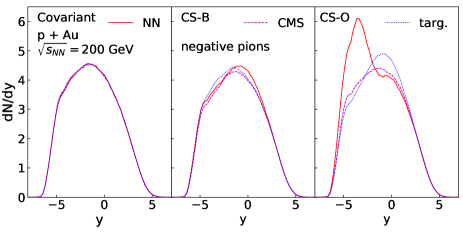
Figure 9: Rapidity dependence of negative pions in p + Au collisions ($b=1$ fm) at $\sqrt{s_{NN}}=200$ GeV from the collision schemes Covariant (left panel), CS-B (middle panel), and CS-O (right panel) are compared for different frames. The equal-speed frame (NN frame), the global c.m.s., and the target frame are plotted by solid, dashed, and dotted lines, respectively.

We now examine asymmetric nuclear collisions. Figure 9 shows the rapidity distribution of negative pions in central p + Au collisions at $\sqrt{s_{NN}}=200$ GeV. The results from the three computational frames—the equal-speed frame of the two colliding nuclei (NN), the global c.m.s., and the target frame—are compared for the collision schemes: covariant, CS-B, and CS-O. It is observed that the results from the three schemes are close to one another in the global c.m.s. The scheme CS-O predictions show strong frame dependence while scheme CS-B does not. The study of the frame dependence in p + Au collisions reveals that non-covariant cascade schemes perform best in the global c.m.s. but not in the equal-speed frame in pA collisions.

IV.4 Cluster separability

In this section, we address the issue of the cluster separability in our covariant cascade scheme. When a system is separated into independent clusters, clusters do not interact with each other in our approach since the timekeeper is a constant vector. However, our scheme does not guarantee the cluster separability in the following sense: When the system is divided into two subsystems with the total momentum of $P_{1}$ and $P_{2}$,

$$P=P_{1}+P_{2},$$ (46)

the cluster separability condition implies that the equations of motion for the system must exhibit two distinct sets of equations,

$$\frac{dq_{i}}{d\tau} =\frac{p_{i}}{\hat{a}_{1}\cdot p_{i}}, \frac{dq_{j}}{d\tau} =\frac{p_{j}}{\hat{a}_{2}\cdot p_{j}},$$ (47)

where $\hat{a}_{1}=P_{1}/\sqrt{P_{1}^{2}}$ and $\hat{a}_{2}=P_{2}/\sqrt{P_{2}^{2}}$. However, this condition is not satisfied in our model. To investigate the effects of cluster separability, we manually impose the cluster separability condition in numerical simulations: when clusters are identified, we incorporate Eq. (47) into the actual simulations. To identify clusters we introduce time steps, and at every time step, we group particles that are close to one another in the coordinate space based on the interaction range.

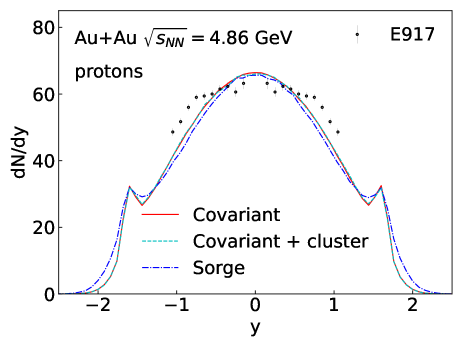
Figure 10: Rapidity distributions in central Au + Au collision at $\sqrt{s_{NN}}=4.86$ GeV are compared with different covariant collision schemes. The solid and dashed lines show the results from the covariant method without and with cluster separation, respectively. The dashed-dotted line corresponds to the results from the covariant method using Sorge’s constraints (19). Experimental data were taken from Back et al. (2002).

The rapidity distribution of protons from our approach is compared with the original covariant method in Fig. 10. We found that our original equations of motion yield the same results as the one that the cluster separability is imposed. As a comparison, the rapidity distribution from the model with Sorge’s constraints (19) is plotted by a dashed-dotted line in Fig. 10, which is in good agreement with our covariant method. Based on these findings, it appears that the issues of cluster separability may not be highly relevant for simulating high-energy nuclear collisions using our approach. However, it is worth noting that when nuclear cluster productions are discussed with the model, such as in the relativistic quantum molecular dynamics, the model incorporating cluster separability may produce more stable clusters. We will leave this topic as a future work.

V Potential interactions

The main ingredients of the QMD model are the Boltzmann-type collision term to simulate hard interactions and the potential interactions for the soft part of the interactions, which play a significant role in determining the collective dynamics of the system. The relativistic version of the QMD (RQMD) model has been developed based on the relativistic constrained dynamics Sorge et al. (1989); Maruyama et al. (1991) using the constraints (19). However, as we mentioned before, accurately solving the constraints (19) is practically infeasible with the current computer capabilities. To address this challenge, RQMD models with the time constraints (33) were proposed Maruyama et al. (1996); Mancusi et al. (2009); Nara and Stoecker (2019); Nara et al. (2020); Nara and Ohnishi (2022), which provide a numerically efficient method. However, these models are limited to the uses in the global c.m.s. We derive covariant equations of motion for the RQMD approach, which allows numerically efficient simulations.

We consider the following mass shell constraints for the particle system interacting through the Lorentz scalar $S_{i}$ and vector $V_{i}$ potentials,

$$H_{i}=p_{i}^{*2}-m_{i}^{*2},\quad i=1,\ldots,N,$$ (48)

where $p_{i}^{*}=p_{i}-V_{i}$ and $m_{i}^{*}=m_{i}-S_{i}$. We use the time constraints of Eqs. (33) and (34). Under the assumption of the approximate commutation of the mass shell constraints $[H_{i},H_{j}]=0$ as in Ref. Sorge et al. (1989), the equations of motions (14) and (15) become

$$\frac{dq^{\mu}_{i}}{d\tau} =\sum_{j=1}^{N}2u_{j}\Pi_{ji}^{\mu}, \frac{dp^{\mu}_{i}}{d\tau} =\sum_{j=1}^{N}2u_{j}Q_{ji}^{\mu},$$ (49)

where

$$\Pi_{ji}^{\mu} =\frac{1}{2}\frac{\partial H_{j}}{\partial p_{i\mu}}=p_{i}^{*\mu}\delta_{ij}-{m_{j}^{*}}\frac{\partial m_{j}^{*}}{\partial p_{i\mu}}-p^{*\nu}_{j}\frac{\partial{V}_{j\nu}}{\partial p_{i\mu}},$$ (50)

$$Q_{ji}^{\mu} =-\frac{1}{2}\frac{\partial H_{j}}{\partial q_{i\mu}}=m_{j}^{*}\frac{\partial m_{j}^{*}}{\partial q_{i\mu}}+p^{*\nu}_{j}\frac{\partial V_{j\nu}}{\partial q_{i\mu}}.$$ (51)

We need to solve the following system of equations for the Lagrangian multipliers $u_{i}$:

$$\sum_{j=1}^{N}(\hat{a}\cdot\Pi_{ji})\,u_{j}=1,\quad i=1,\ldots,N\,.$$ (52)

Let us consider some approximations to avoid solving the system of equations. If we neglect the derivatives of potentials with respect to the energy, we have only the free part, $\hat{a}_{i}\cdot(\partial H_{j}/\partial p_{i})=2p_{i}^{*0}$ in the frame specified by $\hat{a}=(1,0,0,0)$. Thus, the Lagrange multipliers $u_{i}$ are given by $u_{i}=1/(2\hat{a}\cdot p_{i}^{*})$ in any computational frame, and we get the equations of motion

$$\frac{dq^{\mu}_{i}}{d\tau} =\sum_{j=1}^{N}\frac{\Pi_{ji}^{\mu}}{\hat{a}\cdot p_{j}^{*}}, \frac{dp^{\mu}_{i}}{d\tau} =\sum_{j=1}^{N}\frac{Q_{ji}^{\mu}}{\hat{a}\cdot p_{j}^{*}}.$$ (53)

These equations of motion with $\hat{a}=(1,0,0,0)$ are successfully applied in Refs. Nara and Stoecker (2019); Nara et al. (2020); Nara and Ohnishi (2022) for the simulations of heavy-ion collisions.

We expect that the off-diagonal parts of Eq. (52) are small because only one term of the derivatives in the sum of the potentials is non-zero, unlike the diagonal term, in which we need to take the sum for all particles for the derivatives. When we only take the diagonal parts, $u_{i}$ can be obtained trivially as $u_{i}=1/(2\hat{a}\cdot\Pi_{ii})$, and the equations of motion become

$$\frac{dq^{\mu}_{i}}{d\tau} =\sum_{j=1}^{N}\frac{\Pi^{\mu}_{ji}}{\hat{a}\cdot\Pi_{jj}}, \frac{dp^{\mu}_{i}}{d\tau}=\sum_{j=1}^{N}\frac{Q_{ji}^{\mu}}{\hat{a}\cdot\Pi_{jj}}.$$ (54)

We note that the diagonal part $\Pi_{ii}$ is the same as $\tilde{\Pi}_{\mu}$ in Eq. (33) in Ref. Weber et al. (1992). When we take only $j=i$ part of the sum in Eq. (54) in the frame $\hat{a}=(1,0,0,0)$, where all time coordinates of particles are the same as $\tau$, Eq. (54) becomes identical to the equations of motion of the test particles in the relativistic BUU (RBUU) approach Weber et al. (1992). The numerical simulations of the RBUU approach with these equations of motion have been realized for the study of heavy-ion collisions in Ref. Maruyama et al. (1994).

VI Summary

We have presented a Poincaré covariant cascade method that enables efficient numerical simulation of the Boltzmann-type collision term. This method provides an effective approach for accurately modeling and studying collision processes in high energy heavy-ion collisions. We have verified that our covariant cascade method predicts the correct collision rate and the thermal spectrum in a box simulation. Moreover, we have demonstrated the frame independence of our method in a one-dimensionally expanding system as well as actual nuclear collisions, including AA and pA collisions.

Detailed comparisons with the cascade schemes in the $6N$-dimensional phase space have been conducted. It is found that some non-covariant collision schemes can yield reliable results under specific conditions. Specifically, collision scheme CS-O shows reliable results when applied to an expanding system or to the collision of two nuclei with a beam energy less than $\sqrt{s_{NN}}\simeq 20$ GeV. In CS-O, the impact parameter is defined in the two-body c.m.s. of the colliding particles, and the collision time is specified in the computational frame, which is chosen to be the global center-of-mass frame of the two nuclei.

Finally, we proposed numerically efficient covariant equations of motion for $N$-particle systems interacting through potentials, which can be utilized in the QMD simulations at relativistic collision energies.

Appendix A Closest distance approach in $6N$-dimensional phase space

In this appendix, we provide a derivation of the expressions for the impact parameter and the times of the closest approach within a $6N$-dimensional phase space approach. See also Refs. Cheng et al. (2002); Sasaki (2001); Hirano and Nara (2012).

The impact parameter is defined as the minimum distance in the two-body center-of-mass system (c.m.s.),

$$b^{2}=\bm{x}_{\mathrm{cm}}^{2}-\frac{(\bm{x}_{\mathrm{cm}}\cdot\bm{v}_{\mathrm{cm}})^{2}}{\bm{v}_{\mathrm{cm}}^{2}}.$$ (55)

To obtain the Lorentz invariant expression, we define the transverse relative distance $x_{T}$ and the transverse relative momentum $p_{T}$:

$$q_{T} \equiv\Delta^{\mu\nu}q_{\nu}=q-(q\cdot u)u,$$ (56)

$$p_{T} \equiv\Delta^{\mu\nu}p_{\nu}=p-(p\cdot u)u,$$ (57)

where $q=q_{1}-q_{2}$, $p=p_{1}-p_{2}$, $u=\frac{p_{1}+p_{2}}{\sqrt{(p_{1}+p_{2})^{2}}}$, and $\Delta^{\mu\nu}=g^{\mu\nu}-u^{\mu}u^{\nu}$ is the projector to the transverse distances. The impact parameter vector $b$ is orthogonal to the transverse relative momentum $b\cdot p_{T}=0$, which is given by

$$b=q_{T}-\frac{(q_{T}\cdot p_{T})}{p_{T}^{2}}p_{T}=q_{T}-\frac{(q\cdot p_{T})}{p_{T}^{2}}p_{T},$$ (58)

where we used $q_{T}\cdot p_{T}=q\cdot p_{T}$. Then, the square of the invariant impact parameter is evaluated as  Kodama et al. (1984); Sasaki (2001); Hirano and Nara (2012)

$$-b\cdot b=-q_{T}^{2}+\frac{(q\cdot p_{T})^{2}}{p_{T}^{2}}=-q^{2}+(q\cdot u)^{2}+\frac{(q\cdot p_{T})^{2}}{p_{T}^{2}}.$$ (59)

Noting that the relative momentum is proportional to the relative velocity in the c.m.s., this expression is equivalent to Eq. (55) since

$$\bm{x}_{\mathrm{cm}}^{2} =t_{\mathrm{cm}}^{2}-q^{2}=(q\cdot u)^{2}-q^{2},$$ (60)

$$\bm{p}_{\mathrm{cm}}^{2} =E_{\mathrm{cm}}^{2}-p^{2}=(p\cdot u)^{2}-p^{2},$$ (61)

$$\bm{x}_{\mathrm{cm}}\cdot\bm{p}_{\mathrm{cm}} =E_{\mathrm{cm}}t_{\mathrm{cm}}-q\cdot p=q\cdot[(p\cdot u)u-p].$$ (62)

The times of the closest approach are also computed in the two-body c.m.s.:

$$t_{\mathrm{cm}}-t_{\mathrm{cm},1} =-\frac{[\bm{x}_{\mathrm{cm},1}(t_{\mathrm{cm},1})-\bm{x}_{\mathrm{cm},2}(t_{\mathrm{cm},1})]\cdot\bm{v}_{\mathrm{cm}}}{\bm{v}_{\mathrm{cm}}^{2}}$$

$$=-\frac{[\bm{x}_{\mathrm{cm}}-\bm{v}_{\mathrm{cm},2}t_{\mathrm{cm}}]\cdot\bm{v}_{\mathrm{cm}}}{\bm{v}_{\mathrm{cm}}^{2}},$$ (63)

where $t_{\mathrm{cm}}=t_{\mathrm{cm},1}-t_{\mathrm{cm},2}$. Using the relation,

$$\bm{v}_{\mathrm{cm}}=-\bm{p}_{\mathrm{cm},2}\left(\frac{1}{E_{\mathrm{cm},1}}+\frac{1}{E_{\mathrm{cm},2}}\right)$$ (64)

and

$$(\bm{x}_{\mathrm{cm}}-\bm{v}_{\mathrm{cm},2}t_{\mathrm{cm}})\cdot\bm{p}_{\mathrm{cm},2}=x\cdot p_{2}-\frac{t_{\mathrm{cm}}}{E_{\mathrm{cm},2}}p_{2}^{2},$$ (65)

a Lorentz invariant expression of the collision time is obtained as

$$t_{\mathrm{cm}}-t_{\mathrm{cm},1} =\frac{E_{\mathrm{cm},1}}{E_{\mathrm{cm}}}\frac{t_{\mathrm{cm}}p_{2}^{2}-E_{\mathrm{cm},2}(x\cdot p_{2})}{(p_{2}\cdot u)^{2}-p_{2}^{2}}$$

$$=E_{\mathrm{cm},1}\frac{(x\cdot p_{1})p_{2}^{2}-(x\cdot p_{2})(p_{1}\cdot p_{2})}{(p_{1}\cdot p_{2})^{2}-p_{1}^{2}p_{2}^{2}}$$ (66)

where $E_{\mathrm{cm}}=E_{\mathrm{cm},1}+E_{\mathrm{cm},2}=\sqrt{(p_{1}+p_{2})^{2}}$. The times of the closest approach $t_{c1}$ and $t_{c2}$ for the two colliding particles in the computational frame are obtained by Lorentz transforming the collision time

$$t_{c1}-t_{1}=(t_{\mathrm{cm}}-t_{\mathrm{cm},1})\frac{E_{1}}{E_{\mathrm{cm},1}},$$ (67)

which are given by

$$t_{c1} =t_{1}+\frac{p_{2}^{2}(q\cdot p_{1})-(p_{1}\cdot p_{2})(q\cdot p_{2})}{(p_{1}p_{2})^{2}-p_{1}^{2}p_{2}^{2}}E_{1},$$ (68)

$$t_{c2} =t_{2}-\frac{p_{1}^{2}(q\cdot p_{2})-(p_{1}\cdot p_{2})(q\cdot p_{1})}{(p_{1}p_{2})^{2}-p_{1}^{2}p_{2}^{2}}E_{2}.$$ (69)

Appendix B Impact parameter

In this appendix, we show that the impact parameter Eq. (1) is equivalent to the transverse distance at the collision point in the Lorentz covariant cascade method in Eq. (42). From the equations of motion for two particles Eq. (40) and the time of closest approach Eq. (41), the collision point is expressed as

$$q_{c}=q^{\prime}-v_{2}^{\prime}(\tau_{1}-\tau_{2}),$$ (70)

where we have used the relation $v\cdot v_{T}=v_{T}^{2}$, and

$$q^{\prime} =q-\frac{(q\cdot v_{T})}{v_{T}^{2}}v, v^{\prime}_{2} =v_{2}-\frac{(v_{2}\cdot v_{T})}{v_{T}^{2}}v.$$ (71)

The impact parameter vector becomes

$$b =q_{c}-\frac{(q_{c}\cdot P)}{P^{2}}P$$

$$=q_{T}-\frac{(q_{T}\cdot v_{T})}{v_{T}^{2}}v_{T}-v_{2T}^{\prime}\,(\tau_{1}-\tau_{2})$$ (72)

where

$$v_{T2} =v_{2}-\frac{(v_{2}\cdot P)}{P^{2}}P, v_{T2}^{\prime} =v_{T2}-\frac{(v_{T2}\cdot v_{T})}{v_{T}^{2}}v_{T}.$$ (73)

Noting that the transverse relative velocity $v_{T}=v_{T1}-v_{T2}$ is parallel to the transverse velocity of a particle 2 $v_{T2}$,

$$v_{T}\xrightarrow[\text{c.m.}]{}\bm{v}_{\mathrm{cm}}=\bm{v}_{\mathrm{cm},1}-\bm{v}_{\mathrm{cm},2}\approx-\bm{v}_{\mathrm{cm},2},$$ (74)

we can replace $v_{T}$ by $v_{2T}$ in Eq. (73), and one finds $v^{\prime}_{T2}=0$. Furthermore, since $v_{T}$ is also parallel to $p_{T}$, the impact parameter vector becomes

$$b=q_{T}-\frac{(q\cdot v_{T})}{v_{T}^{2}}v_{T}=q_{T}-\frac{(q\cdot p_{T})}{p_{T}^{2}}p_{T},$$ (75)

which is the same expression as the impact parameter vector in the c.m.s. Eq. (58).

References

- Luo et al. (2022) X. Luo, Q. Wang, N. Xu, and P. Zhuang, Properties of QCD Matter at High Baryon Density (Springer Nature Singapore, 2022), ISBN 9789811944406.
- Sorensen et al. (2023) A. Sorensen et al. (2023), eprint 2301.13253.
- Geiger (1997) K. Geiger, Comput. Phys. Commun. 104, 70 (1997), eprint hep-ph/9701226.
- Zhang (1998) B. Zhang, Comput. Phys. Commun. 109, 193 (1998), eprint nucl-th/9709009.
- Molnar and Gyulassy (2000) D. Molnar and M. Gyulassy, Phys. Rev. C 62, 054907 (2000), eprint nucl-th/0005051.
- Xu and Greiner (2005) Z. Xu and C. Greiner, Phys. Rev. C 71, 064901 (2005), eprint hep-ph/0406278.
- Lin et al. (2005) Z.-W. Lin, C. M. Ko, B.-A. Li, B. Zhang, and S. Pal, Phys. Rev. C 72, 064901 (2005), eprint nucl-th/0411110.
- Bertsch and Das Gupta (1988) G. F. Bertsch and S. Das Gupta, Phys. Rept. 160, 189 (1988).
- Aichelin (1991) J. Aichelin, Phys. Rept. 202, 233 (1991).
- Buss et al. (2012) O. Buss, T. Gaitanos, K. Gallmeister, H. van Hees, M. Kaskulov, O. Lalakulich, A. B. Larionov, T. Leitner, J. Weil, and U. Mosel, Phys. Rept. 512, 1 (2012), eprint 1106.1344.
- Sorge et al. (1989) H. Sorge, H. Stoecker, and W. Greiner, Annals Phys. 192, 266 (1989).
- Maruyama et al. (1991) T. Maruyama, S. W. Huang, N. Ohtsuka, G.-Q. Li, A. Faessler, and J. Aichelin, Nucl. Phys. A 534, 720 (1991).
- Xu et al. (2016) J. Xu et al. (TMEP), Phys. Rev. C 93, 044609 (2016), eprint 1603.08149.
- Zhang et al. (2018) Y.-X. Zhang et al. (TMEP), Phys. Rev. C 97, 034625 (2018), eprint 1711.05950.
- Ono et al. (2019) A. Ono et al. (TMEP), Phys. Rev. C 100, 044617 (2019), eprint 1904.02888.
- Colonna et al. (2021) M. Colonna et al. (TMEP), Phys. Rev. C 104, 024603 (2021), eprint 2106.12287.
- Wolter et al. (2022) H. Wolter et al. (TMEP), Prog. Part. Nucl. Phys. 125, 103962 (2022), eprint 2202.06672.
- Zhang and Pang (1997) B. Zhang and Y. Pang, Phys. Rev. C 56, 2185 (1997), eprint nucl-th/9611012.
- Cheng et al. (2002) S. Cheng, S. Pratt, P. Csizmadia, Y. Nara, D. Molnar, M. Gyulassy, S. E. Vance, and B. Zhang, Phys. Rev. C 65, 024901 (2002), eprint nucl-th/0107001.
- Zhao et al. (2020) X.-L. Zhao, G.-L. Ma, Y.-G. Ma, and Z.-W. Lin, Phys. Rev. C 102, 024904 (2020), eprint 2001.10140.
- Kodama et al. (1984) T. Kodama, S. B. Duarte, K. C. Chung, R. Donangelo, and R. A. M. S. Nazareth, Phys. Rev. C 29, 2146 (1984).
- Kortemeyer et al. (1995) G. Kortemeyer, W. Bauer, K. Haglin, J. Murray, and S. Pratt, Phys. Rev. C 52, 2714 (1995), eprint nucl-th/9509013.
- Zhang et al. (1998) B. Zhang, M. Gyulassy, and Y. Pang, Phys. Rev. C 58, 1175 (1998), eprint nucl-th/9801037.
- Welke et al. (1989) G. Welke, R. Malfliet, C. Gregoire, M. Prakash, and E. Suraud, Phys. Rev. C 40, 2611 (1989).
- Lang et al. (1993) A. Lang, H. Babovsky, W. Cassing, U. Mosel, and H. G. Reusch, J. Comp. Phys. 106, 391 (1993).
- Sudarshan et al. (1981) E. C. G. Sudarshan, N. Mukunda, and J. N. Goldberg, Phys. Rev. D 23, 2218 (1981).
- Samuel (1982a) J. Samuel, Phys. Rev. D 26, 3475 (1982a).
- Samuel (1982b) J. Samuel, Phys. Rev. D 26, 3482 (1982b).
- Currie (1963) D. G. Currie, J. Math. Phys. 4, 1470 (1963).
- Currie et al. (1963) D. G. Currie, T. F. Jordan, and E. C. G. Sudarshan, Rev. Mod. Phys. 35, 350 (1963).
- Leutwyler (1965) H. Leutwyler, Nuovo Cim. 37, 556 (1965).
- Maruyama et al. (1996) T. Maruyama, K. Niita, T. Maruyama, S. Chiba, Y. Nakahara, and A. Iwamoto, Prog. Theor. Phys. 96, 263 (1996), eprint nucl-th/9601010.
- Isse et al. (2005) M. Isse, A. Ohnishi, N. Otuka, P. K. Sahu, and Y. Nara, Phys. Rev. C 72, 064908 (2005), eprint nucl-th/0502058.
- Mancusi et al. (2009) D. Mancusi, K. Niita, T. Maruyama, and L. Sihver, Phys. Rev. C 79, 014614 (2009).
- Marty and Aichelin (2013) R. Marty and J. Aichelin, Phys. Rev. C 87, 034912 (2013), eprint 1210.3476.
- Nara and Stoecker (2019) Y. Nara and H. Stoecker, Phys. Rev. C 100, 054902 (2019), eprint 1906.03537.
- Nara et al. (2020) Y. Nara, T. Maruyama, and H. Stoecker, Phys. Rev. C 102, 024913 (2020), eprint 2004.05550.
- Nara and Ohnishi (2022) Y. Nara and A. Ohnishi, Phys. Rev. C 105, 014911 (2022), eprint 2109.07594.
- Nara et al. (2000) Y. Nara, N. Otuka, A. Ohnishi, K. Niita, and S. Chiba, Phys. Rev. C 61, 024901 (2000), eprint nucl-th/9904059.
- Nara (2019) Y. Nara, EPJ Web Conf. 208, 11004 (2019).
- Bass et al. (1998) S. A. Bass et al., Prog. Part. Nucl. Phys. 41, 255 (1998), eprint nucl-th/9803035.
- Sasaki (2001) N. Sasaki, Prog. Theor. Phys. 106, 783 (2001), eprint hep-ph/0009326.
- Hirano and Nara (2012) T. Hirano and Y. Nara, PTEP 2012, 01A203 (2012), eprint 1203.4418.
- Wolf et al. (1990) G. Wolf, G. Batko, W. Cassing, U. Mosel, K. Niita, and M. Schaefer, Nucl. Phys. A 517, 615 (1990).
- Weil et al. (2016) J. Weil et al. (SMASH), Phys. Rev. C 94, 054905 (2016), eprint 1606.06642.
- Danielewicz and Bertsch (1991) P. Danielewicz and G. F. Bertsch, Nucl. Phys. A 533, 712 (1991).
- Cassing (2002) W. Cassing, Nucl. Phys. A 700, 618 (2002), eprint nucl-th/0105069.
- Landau and Lifschits (1975) L. D. Landau and E. M. Lifschits, The Classical Theory of Fields, vol. Volume 2 of Course of Theoretical Physics (Pergamon Press, Oxford, 1975), ISBN 978-0-08-018176-9.
- Staudenmaier et al. (2021) J. Staudenmaier, D. Oliinychenko, J. M. Torres-Rincon, and H. Elfner (SMASH), Phys. Rev. C 104, 034908 (2021), eprint 2106.14287.
- Coci et al. (2023) G. Coci, S. Gläßel, V. Kireyeu, J. Aichelin, C. Blume, E. Bratkovskaya, V. Kolesnikov, and V. Voronyuk, Phys. Rev. C 108, 014902 (2023), eprint 2303.02279.
- Borchers et al. (2000) V. Borchers, J. Meyer, S. Gieseke, G. Martens, and C. C. Noack, Phys. Rev. C 62, 064903 (2000), eprint hep-ph/0006038.
- Peter et al. (1994) G. Peter, D. Behrens, and C. C. Noack, Phys. Rev. C 49, 3253 (1994).
- Behrens et al. (1994) D. Behrens, G. Peter, and C. C. Noack, Phys. Rev. C 49, 3266 (1994).
- Kurkela et al. (2022) A. Kurkela, R. Törnkvist, and K. Zapp (2022), eprint 2211.15454.
- Back et al. (2002) B. B. Back et al., Phys. Rev. C 66, 054901 (2002).
- Ahle et al. (1998) L. Ahle et al. (E-802), Phys. Rev. C 57, R466 (1998).
- Anticic et al. (2011) T. Anticic et al. (NA49), Phys. Rev. C 83, 014901 (2011), eprint 1009.1747.
- Appelshauser et al. (1999) H. Appelshauser et al. (NA49), Phys. Rev. Lett. 82, 2471 (1999), eprint nucl-ex/9810014.
- Afanasiev et al. (2002) S. V. Afanasiev et al. (NA49), Phys. Rev. C 66, 054902 (2002), eprint nucl-ex/0205002.
- Bearden et al. (2004) I. G. Bearden et al. (BRAHMS), Phys. Rev. Lett. 93, 102301 (2004), eprint nucl-ex/0312023.
- Bearden et al. (2005) I. G. Bearden et al. (BRAHMS), Phys. Rev. Lett. 94, 162301 (2005), eprint nucl-ex/0403050.
- Alt et al. (2006) C. Alt et al. (NA49), Phys. Rev. C 73, 044910 (2006).
- Weber et al. (1992) K. Weber, B. Blaettel, W. Cassing, H. C. Doenges, V. Koch, A. Lang, and U. Mosel, Nucl. Phys. A 539, 713 (1992).
- Maruyama et al. (1994) T. Maruyama, W. Cassing, U. Mosel, S. Teis, and K. Weber, Nucl. Phys. A 573, 653 (1994), eprint nucl-th/9307024.