Machine Learning Based Compensation for Inconsistencies in Knitted Force Sensors – Supplement

1 Introduction

This document represents supplementary material for the paper ”Machine Learning Based Compensation for Inconsistencies in Knitted Force Sensors” by Aigner and Stöckl [1]. The following chapters present in-depth plots as well as more detail on transferability of the proposed method to predicting strain instead of force, which was only touched briefly in the paper, to avoid oververbosity.

2 Timeline Plots

We include additional timeline plots, complementary to the ones in the main paper: Figure 1 (top) shows input features $G_{1}$ thru $G_{7}$ for the entirety of our collected data set. It is clearly visible that features with low $\alpha$ increasingly model the long-term drift. The remaining sub-figures show the full timeline plots of both PES and both Lycra test sets, in addition to the close-ups in the full paper.

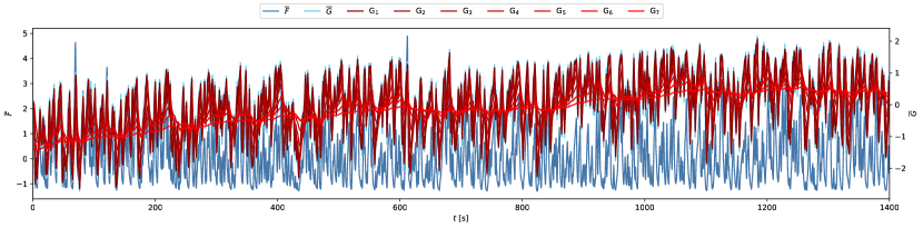
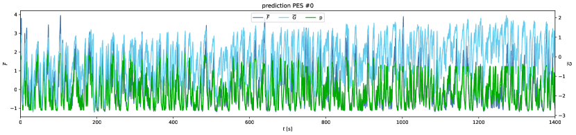
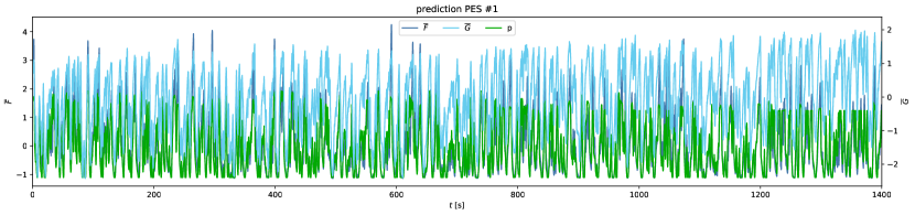
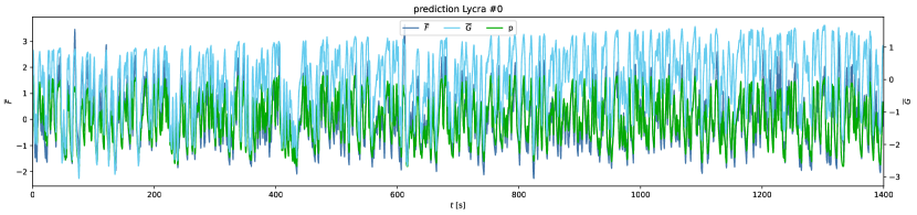
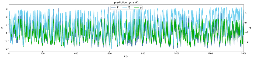
Figure 1: Features $G_{1}$ thru $G_{7}$ of our PES training set (top) and entire prediction results of our test sets.

3 Mapping Sensor Data to Actuator Displacement

As briefly touched in the paper, our technique works for strain/displacement data as well. To achieve the following results we merely trained against normalized displacement $\overline{d}$, by re-sampling actuator displacement (i.e., absolute sensor elongation) $d$ to 20 Hz and then removing mean and scaling to unit variance using the StandardScaler from the scikit learn Python package. We used the exact same pipeline including initialization of $y(0)$ for exponential smoothing filters, as well as neural network hidden layer design, MLPRegressor activation function, etc. Figure 2 shows timeline plots of an exemplary PES (top) and Lycra recordings (bottom).

We can see that $d$ seems to drift along with $G$, however the relative drift differs in between sensor variations. Our method adapts well to these differences: $r^{2}$ values (pre- and post-prediction) can be found in Table 1, which shows considerable gain in mapping between sensor conductivity and elongation when applying our method, with highest gains for PES patches.

Note that the model was not at all manually adapted to the different objective; in preliminary experiments, we found that by changing the NN’s hidden layers, we could slightly improve test scores up to 0.716. However, we believe those minor differences are subject to the training set and do not make a crucial difference in real-world applications.

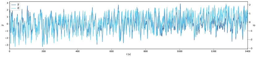
(a)

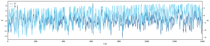
(b)

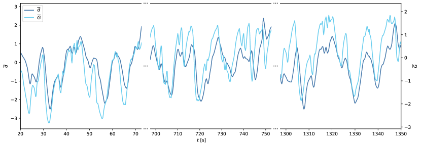
(c)

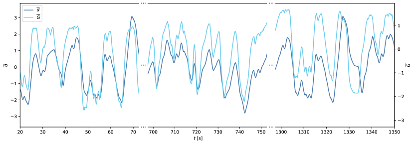
(d)

Figure 2: Plots showing $\overline{d}$ and $\overline{G}$ of PES #0 (a,b) and a Lycra #0 (c,d) test sets.

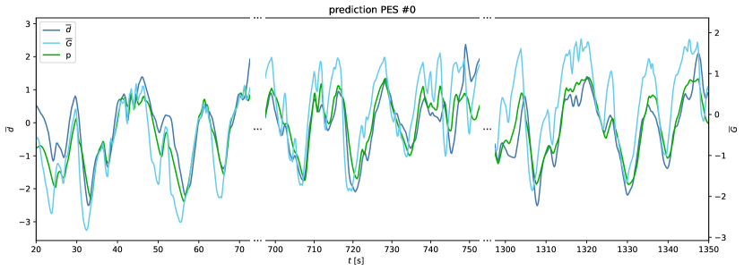
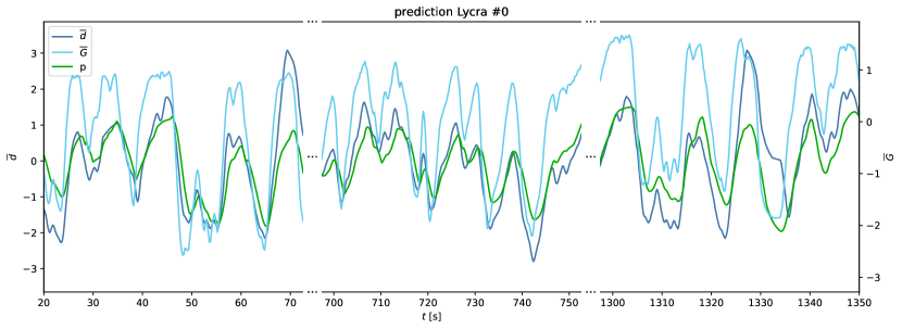
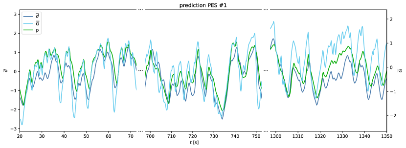
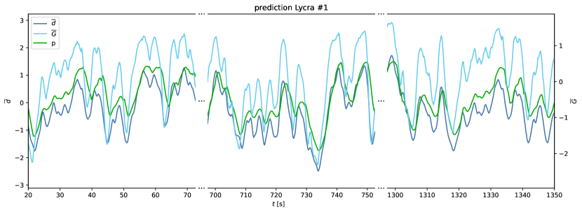
Figure 3: Resulting predictions $p$ show good rectification of the input signals for all of our test sets, although we can observe occasional under-estimations of peak areas in the signal, as is the case when predicting force data (see main paper).

4 Notes on Enclosed Spreadsheet

In order to compare model in terms of their performance on both test sets A and B, we calculated an error metric $E$ from the respective $r^{2}$ scores with

$$E=\frac{(1-r^{2}_{A})^{2}+(1-r^{2}_{B})^{2}}{2}\,.$$

Values reported and color-coded in the enclosed spreadsheet nn-eval.xlsx represent according $E$-values, i.e., values close to 0 indicate better performance.

Table 1: $r^{2}$ of our initial (pre-processed) and predicted data when applied to actuator displacement. We included results of our two test sets (A, B), as well as the training sets (T) for sake of completeness. PES show highest gain from our approach, however, the Lycra patches ultimately yield higher scores.

	r²(d,G)	r²(d,p)	gain
PESt	0.319	(0.705)	(0.386)
PESA	0.319	0.699	0.380
PESB	0.260	0.635	0.375
Lycrat	0.337	(0.687)	(0.350)
LycraA	0.479	0.609	0.130
LycraB	0.490	0.669	0.179

5 Data Processing Pipeline

Figure 4 shows the data processing steps that are involved for both acquiring data from the sensors on the MCU, as well as during pre-processing for training the ANNs in Python. Load cell as well as knitted sensors were sampled using two Delta-Sigma ADCs by a single ESP32 MCU. Resistance values read from the load cell were converted to Newtons already in the firmware. Since resistance readings of the textile sensor were slightly noisier, we supersampled with 128 Hz, buffered values and calculated mean values in the firmware every 25 ms. Since timing on the firmware could not be controlled to achieve periods of 25 ms precisely, we resampled to constant frequency in Python later based on the timestamps that were recorded to the CSV file along the sensor readings. Furthermore, resistance values $R$ were inverted to get conductivity values $G$. To achieve better performace of the machine learning estimators to be used, we normalized both $F$ and $G$ uniform ranges using the scikit learn StandardScaler, which centers data round $\mu$ and scales with $1/\sigma$.

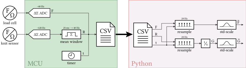
Figure 4: During data recording, values of knitted sensors are super-sampled and in order to reduce measurement noise. Within time windows of 25 ms, mean values are calculated and written to CSV files, along timestamps and data sampled from the load cell. During pre-processing for training our ML models, data is resampled to unified time periods between samples, since our proof-of-concept does not yet take timing into account, for reasons of simplicity.

References

- [1] R. Aigner and A. Stöckl, “Machine learning based compensation for inconsistencies in knitted force sensors,” 2023.