Accelerating Multiframe Blind Deconvolution via Deep Learning

1 Introduction

sec:Introduction

Ground-based solar observations are affected by aberrations caused by the turbulent nature of Earth’s atmosphere. Although moving the telescope to space is feasible, it is expensive. That is the reason why correction methods have been developed to improve ground-based observations. Real-time adaptive optics (AO) measure the distortion of the wavefront using wavefront sensors in real-time and try to compensate for it using deformable mirrors. Once measured, a-posteriori software methods push the quality further.

Although AO systems can remove a substantial amount of aberrations in real-time, they still suffer from limitations. The corrections are not perfect because of the lag between the measurement of the wavefront and the correction. This leads to some perturbations remaining in the science images, which cannot reach the diffraction limit of the telescope. Additionally, single-conjugate AO systems, which are available in the majority of solar telescopes, only correct the turbulence in the pupil of the telescope, whose influence is the same for the whole field-of-view (FoV). The presence of turbulence at higher layers in the Earth’s atmosphere produces differential aberrations in different regions of the FoV.

To achieve the diffraction limit of the telescope, it is crucial to remove residual aberrations, which can only be practically achieved with a-posteriori correction methods. Since neither the instantaneous state of the atmosphere nor the unaberrated object are known, all a-posteriori methods belong to the class of blind deconvolution algorithms. In these algorithms, prior information is used to simultaneously solve for the object and the atmospheric aberrations, a problem that is known to be ill-defined. The application of these methods requires specific observing strategies. The main requisite is to observe a sufficiently large burst of images of low quality that can later be combined to produce an image of improved quality. One requires the exposure time of these individual frames to be faster than the coherence time of the atmosphere in order to freeze the atmosphere. For a typical observing day, the integration time needs to be as small as a few milliseconds. Although of excellent performance, unfortunately, these methods are computationally demanding. They require the maximization of a likelihood (or posterior if priors are used) with respect to the instantaneous point spread functions (PSF) and the object.

Arguably the simplest a-posteriori correction method is that of lucky imaging or frame selection. This requires the definition of a metric measuring the quality of each individual image and only selecting the best one that maximizes the metric. Although effective in some cases (e.g., Oscoz et al., 2008), they make a very limited use of the available information because they do not combine low-quality frames for the sake of producing an improved image. More elaborate techniques, like speckle methods (Labeyrie, 1970; von der Lühe, 1993), do make use of all frames and try to estimate a high-quality image exploiting the statistics of the atmospheric turbulence. Arguably, a step forward happened when Paxman, Schulz, and Fienup (1992) proposed a blind deconvolution method based on three main pillars. The first one is a consistent model for the PSFs, which is of special interest for telescopic observations. This model is obtained by a linear expansion of the wavefront in the pupil in a suitable basis (Zernike polynomials and Karhunen-Loève modes are the two most used basis). The PSF is obtained as the autocorrelation of the pupil function (see section sec:mfbd for more details), which naturally leads to positive defin ite PSFs in which diffraction is automatically taken into account. The second pillar is a proper treatment of the noise through a Bayesian approach. The function to be optimized, the likelihood, depends on the assumed noise statistics. Finally, the third pillar is the use of phase-diversity techniques (Gonsalves and Chidlaw, 1979) to better inform the optimization. The idea behind phase-diversity is to simultaneously acquire an image with a known aberration, which is used to constrain the optimization. Based on this approach, Löfdahl and Scharmer (1994) and Löfdahl et al. (1998) applied the phase-diversity (image correction with only two simultaneous images, one at focus and the other one with a known defocus) approach to solar observations. Later, Löfdahl et al. (2002) proposed to use many short exposure frames (multi-frame approach) to solve the blind deconvolution problem. Each frame is affected by different aberrations although they come from the same object. Both approaches were very successful, and were later combined and expanded by van Noort, Rouppe van der Voort, and Löfdahl (2005). These authors considered, apart from having many frames with phase diversity, the presence of many objects (multiobject), typically made of observations at different wavelengths. These objects are obtained simultaneously and assumed to be affected by the same aberrations. They developed the multiframe multiobject blind deconvolution code (MOMFBD), which is now routinely used in solar observations.

Given the high computational requirements of multi-frame (multi-object) blind deconvolution classical methods, Asensio Ramos, de la Cruz Rodríguez, and Pastor Yabar (2018) investigated the use of learning-based methods that leverage neural networks to correct atmospheric influences quickly. They proposed two large convolutional neural networks (CNNs) to correct a burst of images and produce a frame of higher quality. The CNNs were trained supervisedly with observations of the Swedish 1-m Solar Telescope (SST; Scharmer et al., 2003), which were previously corrected with the MOMFBD code. This approach can correct observations as large as 1k$\times$1k at a cadence of 100 images per second, close to real-time, neglecting the mandatory standard data reduction. Although this approach is promising for real-time image correction, it has two main disadvantages. The first one is that the training requires a previous run of the time-consuming MOMFBD code. The second is that only corrected images are obtained, and no information about the instantaneous wavefront (or PSF) is inferred, which may prevent correcting other simultaneous data obtained at other wavelengths.

Later, Asensio Ramos and Olspert (2021) realized that a neural model can be trained simply from corrupted images by making use of the physics of image formation inside the model. The neural network is then responsible for predicting the instantaneous PSFs, instead of the corrected images. Leveraging the linear theory of image formation and using the loss function utilized in the MOMFBD code, which only depends on observed corrupted images, the training can be done in a fully unsupervised manner. Apart from the advantage of unsupervised training, this approach also allows the PSFs to be reused for correcting other instruments observing in perfect synchronization in the same FoV. With the advent of new telescopes, using several instruments to observe the same FoV at the same time will become widespread.

It seems obvious that machine learning-assisted deconvolution is one of the possible avenues for improving the quality and speed of solar blind deconvolution. This is of special relevance given the large amount of large-scale observations that we are currently gathering with current telescopes like the SST at the Observatorio del Roque de los Muchachos (Spain), the GREGOR telescope (Schmidt et al., 2012; Kleint et al., 2020) at the Observatorio del Teide (Spain), the Goode Solar Telescope (GST) on the Big Bear Observatory (USA) or the Daniel K. Inouye Solar Telescope on the Haleakala Observatory (USA). Future telescopes, like the European Solar Telescope (EST), will produce an even larger amount of data that needs to be corrected quickly.

In this paper, we propose two novel ideas. The first one is a set of improvements over the model proposed by Asensio Ramos and Olspert (2021), which arguably produces better results. The second one is an approach for image reconstruction based on algorithm unrolling. This approach is, in spirit, much closer to the classical MOMFBD optimization approach.

2 Multi-frame Blind Deconvolution

sec:mfbd The formalism followed in this paper is similar to that of Asensio Ramos and Olspert (2021), although with some small but important differences. Let us assume that we collect $J$ short exposure frames with a ground-based instrument of a stationary object outside Earth’s atmosphere. In our case, given our scientific interests, our object is a small region on the surface of the Sun. The exposure time of each individual frame is short enough –of the order of milliseconds– so that one can assume that the atmosphere is “frozen”, i.e., it does not evolve during the integration time. Additionally, the total duration of the burst of exposures has to be shorter than the solar evolution timescales, so that the object can be safely assumed to be the same for all frames. From the linear theory of image formation, for a spatially invariant system, the image $i_{kj}$ registered on a sensor can be expressed as a convolution of the true object $o_{k}$ with the PSF of the optical system and atmosphere, that we denote as $s_{kj}$, plus photon noise $n_{kj}$:

$$i_{kj}(r)=o_{k}(r)*s_{kj}(r)+n_{kj}(r),\ilabel{eq:gen_{m}odel}$$ (1)

where $r=(x,y)$ represents the coordinates on the image plane and $j\in\{1\dots J\}$ labels each individual frame for object $k\in\{1\dots K\}$. We make the assumption that all $K$ objects are observed strictly simultaneously, so that they share the same atmospheric perturbations. In the standard case of photon noise, the noise can be assumed to be Poissonian. However, in the regime of high signal-to-noise ratio (S/N), like in the case of our observations, it rapidly converges to a Gaussian statistics. This assumption greatly simplifies the solution of the problem, as shown below.

The task of MOMFBD is to restore the object $o$ from the measurement of all frames $i_{j}$. However, the problem is indeed blind, since both $o$ and all $s_{j}$ are unknown. Such problem can only be solved in the Bayesian framework. From a Bayesian perspective, our aim is to compute the posterior distribution over the object and the PSFs conditioned on the observations, $p(\mathbf{o},\mathbf{s}|\mathbf{i})$, which can be computed as:

$$p(\mathbf{o},\mathbf{s}|\mathbf{i})\propto p(\mathbf{i}|\mathbf{o},\mathbf{s})p(\mathbf{o},\mathbf{s}),$$ (2)

where $p(\mathbf{i}|o,\mathbf{s})$ is the likelihood function and $p(o,\mathbf{s})$ is the prior distribution. The likelihood function takes into account the information encoded in the data, while the prior encodes all explicit a-priori knowledge about the object and the PSFs. One widespread solution to the blind deconvolution problem is the one that maximizes the posterior, commonly known as maximum a-posteriori (MAP) solution:

$$\arg\max_{\mathbf{o},\mathbf{s}}p(\mathbf{i}|\mathbf{o},\mathbf{s})p(\mathbf{o},\mathbf{s}).\ilabel{eq:map}$$ (3)

Prior information can also be incorporated implicitly. In general, one can define a flat prior in the pixel space and allow the optimization to find the instantaneous PSFs. However, this does not work well in practice because of the enormous freedom. For this reason, it is useful to reduce the space of PSFs in which the optimization will search. Following the standard approach in the solar application of MOMFBD, we regularize the solution by assuming that the PSF is obtained via the wavefront entering the pupil of the telescope. We introduce the generalized pupil function $P_{j}$, so that the PSF can be obtained as the autocorrelation of the generalized pupil function:

$$P_{kj}(v) = A_{k}(v)e^{i\varphi_{kj}(v)},$$ (4)

$$s_{kj} = |\mathcal{F}^{-1}(P_{kj})|^{2},$$ (5)

where $A(v)$ is the mask of the telescope aperture (that includes the shadow of the secondary mirror or any spider if present), $\varphi_{kj}$ is the phase of the wavefront, $v$ is the coordinate on the pupil plane and $\mathcal{F}^{-1}$ denotes the inverse Fourier transform. Note that $i$ refers to the imaginary unit number.

As mentioned above, the wavefronts are parameterized through suitable basis functions. In this study we use the Karhunen-Loève basis (e.g., van Noort, Rouppe van der Voort, and Löfdahl, 2005), which makes the expansion coefficients statistically independent under the assumption of Kolmogorov turbulence. This can potentially help regularize the inversion problem by making the coefficients of the wavefront more independent. The wavefront can be expressed as (van Noort, Rouppe van der Voort, and Löfdahl, 2005):

$$\varphi_{kj}(v)=\sum_{l=1}^{M}\alpha_{jl}{\rm KL}_{l}/\lambda_{k},\ilabel{eq:wavefront}$$ (6)

where $M$ is the number of basis functions and $\alpha_{jl}$ is the coefficient associated with the basis function $\mathrm{KL}_{l}$ of the $j$-th atmospheric frame. In all experiments carried out in this paper, we use $M=44$, which gives excellent results in the recovery of the object. In all the results shown in this paper, all objects are observed very close in wavelength. This simplifies the problem and one can drop the wavelength normalization in Eq. (eq:wavefront).

We assume flat priors for the KL coefficients and the object $o$. We also assume that all measured frames $\mathbf{i}$ are statistically independent, so that the likelihood function factorizes. Taking into account the generative model of Equation (eq:gen_model), the solution of Equation (eq:map) can be obtained by optimizing the following quantity (commonly known as loss):

$$L(o,\mbox{\boldmath$\alpha$})=\sum_{k,j,r}\gamma_{kj}\left[i_{kj}(r)-o_{k}(r)*s_{kj}(r,\bm{\alpha}_{j})\right]^{2},\ilabel{eq:loss}$$ (7)

where $\gamma_{j}$ is the inverse variance of the photon noise and the summation over $r$ is over all pixels of the image. The same log-likelihood can be computed in the Fourier domain, which significantly simplifies it by removing the convolution:

$$L(o,\mbox{\boldmath$\alpha$})=\sum_{k,j,u}\gamma_{kj}\left[I_{kj}(u)-O_{k}(u)S_{kj}(u,\bm{\alpha}_{j})\right]^{2},\ilabel{eq:loss_{f}ourier}$$ (8)

where, in this case, $u$ represents frequencies in the Fourier domain, $I_{kj}=\mathcal{F}(i_{kj})$ and $S_{kj}=\mathcal{F}(s_{kj})$, the latter being known as the optical transfer function (OTF).

The simultaneous optimization of the loss functions of Equations (eq:loss) or (eq:loss_fourier) with respect to the object and the PSFs is complicated because of its nonconvexity. To this end, we use an alternating optimization method, already used in this field by Paxman, Schulz, and Fienup (1992). If the wavefront coefficients are known, the loss function is linear in the object and can be analytically estimated using, for instance, a Wiener filter:

$$\overline{O}_{k}(u)=\frac{\sum_{j}\gamma_{kj}I_{kj}(u)S^{*}_{kj}(u,\bm{\alpha}_{j})}{\sum_{j}\gamma_{kj}|S_{kj}(u,\bm{\alpha}_{j})|^{2}+\frac{S_{n}}{S_{0}(u)}},\ilabel{eq:wiener}$$ (9)

where the overline indicates that this is an estimated quantity, while $S_{n}$ is the noise power spectrum and $S_{0}(u)$ is the estimated power spectrum of the object. Arguably, the simplest version of the Wiener filter assumes that $S_{n}/S_{0}(u)$ is constant and independent of the frequency. Although this gives good results, it was demonstrated by Paxman, Schulz, and Fienup (1992) and Löfdahl and Scharmer (1994) that improved images can be obtained by applying a Fourier filter that is a function of the Fourier coordinates $u$:

$$\overline{O}_{k}(u)=H_{k}(u)\frac{\sum_{j}\gamma_{kj}I_{kj}(u)S^{*}_{kj}(u,\bm{\alpha}_{j})}{\sum_{j}\gamma_{kj}|S_{kj}(u,\bm{\alpha}_{j})|^{2}},\ilabel{eq:object}$$ (10)

being $H$ a filter with the following form:

$$H_{k}(u)=1-\frac{\sum_{j}|S_{kj}(u,\bm{\alpha}_{j})|^{2}}{|\sum_{j}I_{kj}(u)S_{kj}(u,\bm{\alpha}_{j})|^{2}},$$ (11)

where all values below 0.2 are set to zero and all values above 1 are set to one. Finally, all isolated peaks in the filter that are not connected with the peak at $u=0$ are removed after applying a median filter with a $3\times 3$ kernel.

Once the estimated objects are obtained, the loss function of Equation (eq:loss) does only depend on the wavefront coefficients and can be more easily optimized. To this end, one can use any optimizers for a nonlinear scalar function.

3 The Models

sec:models We propose here two neural approaches to accelerate the blind deconvolution problem in extended objects like the Sun. The first one is based on algorithm unrolling. The second one is an improvement over the model proposed by Asensio Ramos and Olspert (2021), in which the recurrent layers are replaced by convolutional layers and a much deeper convolutional encoder is used to extract features from the images. We warn the reader that we do not claim that the architectures described in the following are optimal in terms of simplicity, efficiency, and accuracy.

3.1 Model 1: Algorithm Unrolling

sec:unrolling Algorithm unrolling (Gregor and LeCun, 2010) consists of serializing (or unrolling) any iterative method for a fixed number of iterations and treating it as a deep model. In principle, algorithm unrolling can be applied to any iterative algorithm and is often used with computational purposes in mind, because certain operations can be parallelized or fused depending on the specific hardware in which it is run. However, it can also be used to improve the convergence of the algorithm if neural networks are placed at certain positions in the unrolled algorithm. Since the majority of optimization algorithms and neural networks are differentiable, the resulting model can be trained using backpropagation. This approach provides a transparent way of mixing together classical iterative algorithms and neural networks (see Monga, Li, and Eldar, 2021, for a recent review).

Following the steps described in the previous section, we propose to solve Equation (eq:loss) repeating the following scheme a fixed number of times $K$:

• Assume that the wavefront coefficients are known and estimate the object using Equation (eq:object).

• Assume that the object is known and carry out a correction of the wavefront coefficients using a gradient descent step. This requires the computation of the gradient of the loss function with respect to the wavefront coefficients:

  $$\mbox{\boldmath$\alpha$}_{i+1}=\mbox{\boldmath$\alpha$}_{i}-\eta_{i}\nabla L(o,\mbox{\boldmath$\alpha$}_{i}),\ilabel{eq:gradient_{d}escent}$$ (12)

  where the gradient is taken with respect to $\alpha$ and $\eta_{i}$ acts as a learning rate. This gradient can be computed analytically using the chain rule or using automatic differentiation.

This iterative scheme is known to converge slowly. Following the inspiration of Gregor and LeCun (2010), we propose to modify Equation (eq:gradient_descent) to:

$$\mbox{\boldmath$\alpha$}_{i+1}=\mbox{\boldmath$\alpha$}_{i}-\eta_{i}F_{i}(\mbox{\boldmath$\alpha$}_{i},\nabla L(o,\mbox{\boldmath$\alpha$}_{i})),\ilabel{eq:gradient_{d}escent_{n}eural}$$ (13)

where the $F_{i}$ are (potentially different) $K$ neural networks that take as input the current estimation of the wavefront coefficients and the gradient of the loss function and output the correction to be applied to the wavefront coefficients. We found that the order of magnitude of the coefficients and the gradients were not so different, so that they enter into the neural network without any extra compensation. Anyway, we would like to explore in the future the option of adding a learnable weight to the gradients to see if it improves the results. A graphical representation of the unrolled model is displayed in Fig. fig:nn_unroll. After each iteration, one can compute a loss function $L_{i}$, which is computed with the current estimation of the object $O_{i}$ and the wavefront coefficients $\mbox{\boldmath$\alpha$}_{i}$. Typically, the weights of the neural networks and the values of the learning rates are trained end-to-end by minimizing the sum of these losses for the $K$ steps.

When carrying out the training in acceleration hardware like GPUs, one can potentially find memory limitations. To overcome these limitations, we propose here to use a greedy training of the neural networks, which consists of updating the weights of each individual neural network one after the other. To this end, after the first step of the unrolled gradient descent method and the first neural network, one has all the ingredients to compute the loss function. At this point, one can update the weights of the neural network $F_{1}$ using the gradient of $L_{1}$ with respect to the weights of the neural network. After this step, one can update the weights of the neural network $F_{2}$ using the gradient of $L_{2}$ with respect to the weights of the neural network $F_{2}$ and so on. This process is repeated until the weights of all the neural networks have been updated. The memory footprint of this approach is much lower than the end-to-end approach and it is also much faster to train. Although it can lead to a potentially slightly lower accuracy, we verified in a limited amount of comparisons that this lower accuracy does not significantly impact the results.

In our model, each neural network $F_{i}$ is a 1D convolutional neural network acting on the time direction. The current estimation of the wavefront coefficients and the gradient of the loss function are concatenated producing a tensor of size $B\times 2M\times J$, where $B$ is the batch size, $M$ is the number of coefficients and $J$ is the number of frames. This tensor is then passed through two 1D convolutional layers with $2M$ filters of size $3$ and stride $1$ with Gaussian Error Linear Unit activation functions (GELU; Hendrycks and Gimpel, 2016). At the end, a final convolutional layer produces again a tensor of size $B\times M\times J$ with the wavefront coefficients for all the images in the burst. After a non-exhaustive search for the optimal number of unrolling steps, we stick to $K=10$. This gives a total amount of 816.2k trainable parameters, divided into the ten 1D CNNs.

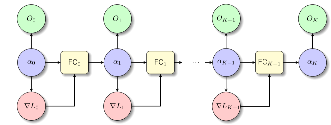
Figure 1.: Scheme of the unrolled model. The estimated wavefront coefficients $\mbox{\boldmath$\alpha$}_{i}$ are used to compute the gradient of the loss function, $\nabla L_{i}$, which also needs the estimated object $O_{i}$. Both the coefficients and the gradients are refined by a neural network that produces updated wavefront coefficients. The training proceeds by forcing these neural networks to produce wavefront coefficients that are as close to the solution as possible at each step of the unrolled algorithm.fig:nn˙unroll

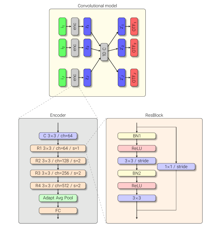
Figure 2.: Convolutional model (upper panel). The Resnet18 encoder architecture is displayed in the gray block. The ResBlock that is part of the Resnet18 model is displayed in the orange block. C: convolutional layer, R: ResBlock, FC: fully connected, BN: batch normalization, ReLU: rectified linear unit.fig:nn˙cnn

3.2 Model 2: Fully Convolutional

sec:unsupervised The second model we investigate in this work is an update of the one proposed by Asensio Ramos and Olspert (2021). The model is displayed in the upper panel of Fig. fig:nn_cnn. The observed $M$ frames are passed through a common convolutional encoder to extract features. We propose to change the relatively simple encoder used by Asensio Ramos and Olspert (2021) to a Resnet18 (He et al., 2015). We found that such a deep network is able to extract relevant features even from single images when a second channel with a phase diversity does not exist. This neural network is in charge of extracting relevant features that allow the model to estimate the wavefront coefficients. Therefore, the specific solar structure that is observed in each case has to be ignored by the neural network. The architecture of the Resnet18 is found in the lower left panel of Fig. fig:nn_cnn. An initial convolutional layer with $64$ filters of size $3\times 3$ is followed by the consecutive application of residual blocks (ResBlock), whose architecture is displayed in the lower right panel of Fig. fig:nn_cnn. The size of the input image is decreased by a factor of $2$ after each ResBlock with a stride of 2. An adaptive average pooling produces an output that is independent of the size of the input images. A final fully connected layer produces the latent vector $z_{i}$ for each image $i$, whose length is equal to the number of KL modes considered in the wavefront. We train the encoder from scratch.

Instead of combining the latent vectors $z_{i}$ using a Gated Recurrent Unit as proposed by Asensio Ramos and Olspert (2021), we prefer to use another convolutional neural network (attention layers are also perfectly good candidates that need to be explored in the future). To this end, all latent vectors $z_{i}$ are combined into a tensor of size $B\times M\times J$. This tensor is then passed through a simple convolutional neural network made by the consecutive application of two 1D convolutional layers with $2M$ filters of size $3$ and stride $1$, followed by GELU activation functions. A final convolutional layer produces again a tensor of size $B\times M\times J$. The role of this CNN is to couple together all wavefront coefficients to partially take into account their temporal correlation for all the frames in a single burst. From these wavefront coefficients, the OTFs and the MOMFBD loss are computed.

The total number of trainable parameters is 11.2M, where roughly 99% of the parameters correspond to the Resnet18 encoder, while the remaining 1% of the parameters belong to the CNN that combines all latent vectors to share temporal information.

3.3 Preprocessing

set:preprocessing The calculation of the deconvolved image with the Wiener filter of Equation (eq:object) requires the Fourier transform of the observed images. Since they are not periodic, and in order to avoid the appearance of spurious high frequencies in the final result, we apodize them with a Hanning window of 12 pixels in each border.

We note that it is crucial to properly normalize the input of the neural networks. In the case of the second model, the input to the Resnet18 encoder are the images themselves. For this reason, we preprocess the images by transforming them to the $[0,1]$ interval using the minimum and maximum brightness in the burst. The images enter into the encoder unapodized. The neural networks of the unrolled model deal directly with the wavefront coefficients. Specifically, these coefficients are never too large in the case of datasets of outstanding quality, so only then can the wavefront coefficients be entered into the neural networks without additional normalization.

In order to avoid dealing with very large tip-tilts, the observed bursts are first destretched. This is done by computing local tip-tilts in a coarse grid using cross-correlation. The frames are realigned by reinterpolation using bilinear interpolation. Once the coarse destretching is complete, additional steps with finer grids deal with the small-scale alignment. Although it is not specially time-consuming and results almost negligible in the case of classical deconvolution algorithms, this prealignment takes a large fraction of the computing time when using our neural approaches. We plan to train neural networks in the future to estimate the optical flow for destretching and to carry out this step as close to real-time as possible.

3.4 Tip-tilt Handling

sec:tip_tilt In general, and specially when the observed objects fill the entire FoV, it is not possible to infer an absolute tip-tilt. The fundamental reason is that tip-tilt enters the OTF as a phase factor, thus it is obvious that only relative tip-tilt between different frames can be estimated. Fortunately, this can be solved using different strategies. If sufficiently long bursts are obtained, one can force the mean tip-tilt to be zero and obtain the relative tip-tilts of all frames with respect to the mean. Another option is to set the tip-tilt of the first (or any) frame to zero and infer the tip-tilt of every frame with respect to the first one (or the one selected as reference). We have chosen the first option, which gives good results.

4 Training

sec:training Both neural models are trained using a combination of data coming from the SST and GREGOR. Since the physics of image formation is part of the loss function, both models can be trained fully unsupervisedly using only observations, following the same strategy described by Asensio Ramos and Olspert (2021) describe the training data in the following.

4.1 SST Data

sec:sst We used high-spatial-resolution observations of diverse structures taken with the SST. These datasets were obtained in common photospheric and chromospheric diagnostics during our 2019 and 2020 campaigns. Table 1 outlines observing details of each dataset.

Table 1.: Observing details of the SST datasets: date, target (QS: Quiet Sun, EN: Enhanced Network, AR: Active Region, PL: Plage), FoV center at the beginning of the observation, observed spectral lines, temporal cadence, and for what the data were used.tab:obs˙sst˙1

Date	Target	Position	Spectral lines	Cadence	Use
		(x, y)		[s]
01–Aug–19	QS	(1”, 0”)	Ca ii 854.2 nm	31	Training
01–Aug–19	QS	(2”, –58”)	Ca ii 854.2 nm	31	Validation
01–Aug–19	EN	(110”, 10”)	Ca ii 854.2 nm	31	Training
26–Jul–20	AR	(-220”, –416”)	Fe i 617.3 nm	60	Training
			Ca ii 854.2 nm	60
			Ca ii K 393.4 nm	6
27–Jul–20	AR	(-20”, –416”)	Ca ii 854.2 nm⋆	20	Validation
			Ca ii K 393.4 nm	6
06–Aug–20	PL	(-115”, 315”)	Fe i 617.3 nm	50	Training
			Ca ii 854.2 nm	50
			Ca ii K 393.4 nm	9

We acquired spectropolarimetric data in the Fe i 617.3 nm and Ca ii 854.2 nm spectral lines with the CRisp Imaging Spectropolarimeter (CRISP; Scharmer, 2006; Scharmer et al., 2008). Among other elements, its optical system includes three synchronized CCD cameras: two cameras collect pairs of narrowband images with orthogonal polarization states while another camera records wideband images that offer context information and act as anchor images during the restoration process with the MOMFBD technique. All cameras obtain images with short time exposure (17 ms) to record data where seeing-induced distortions are frozen. The sampling of each spectral line was narrow at the line core and broader at the line wings (see Table 2). We note that we used two different samplings for the Ca ii 854.2 nm line. The temporal cadences specified in Table 1 thus result from the number of accumulations (in Table 2), the exposure time, and the acquisition of four modulation states. Each CRISP image has a FoV of 55”$\times$55” ($\sim$960$\times$960 pixels) with a plate scale of 0.057”.

Table 2.: Sampling of the spectral lines observed with CRISP and CHROMIS and the number of accumulations. Wavelength positions within the square brackets are indicated from the line center.tab:obs˙sst˙2

Spectral lines	Acc.	Wavelength positions [mÅ]
Fe i 617.3 nm	12	[0, $\pm$30, $\pm$60, $\pm$90, $\pm$120, $\pm$150, $\pm$180]
Ca ii 854.2 nm	12	[0, $\pm$65, $\pm$130, $\pm$195, $\pm$260, $\pm$325, $\pm$390, $\pm$520,
		$\pm$650, $\pm$845, $\pm$1.040, $\pm$1.755]
Ca ii 854.2 nm⋆	12	[0, $\pm$65, $\pm$130, $\pm$260, $\pm$520, $\pm$780, $\pm$1.040, $\pm$1.755]
Ca ii K 393.4 nm	15	[0, $\pm$65, $\pm$130, $\pm$195, $\pm$260, $\pm$325, $\pm$390, $\pm$455,
		$\pm$520, $\pm$585, $\pm$650, $\pm$845, $\pm$1235] + extra point at 400 nm

The Ca ii K data were obtained with the CHROMospheric Imaging Spectrometer (CHROMIS; Scharmer, 2017). In contrast to CRISP, CHROMIS only provides intensity data at different wavelength positions so far. The optical system of CHROMIS also contains three CCD cameras, of which one collects narrowband images while the other two record wideband data. Specifically, one of the wideband cameras also collects data with a defocus (to carry out deconvolution using phase diversity), which turns out to be essential for improving the image restoration quality (Löfdahl et al., 2021). We do not make use of this channel in this work, but the neural models can be trivially modified to include it. CHROMIS images have also a short time exposure (1–2 ms). Their FoV is of 72”$\times$45” ($\sim$1900$\times$1200 pixels) with a pixel size of 0.038”.

We applied a basic data reduction, i.e., images in each dataset are aligned and corrected for dark and flat-field. In the case of the Ca ii 854.2 nm data, we performed additional processing to the flat-field data because these datasets show the imprint of the camera electronics, showing a circuit-like pattern. This pattern is visible in infrared observations acquired until August 2022 because of the decrease in the efficiency of the CCD cameras at such wavelengths. A traditional flat-field correction is insufficient to eliminate this pattern, so flat-field data processed considering the backscatter problem are necessary. More details on the backscatter problem of the CCD cameras can be found in de la Cruz Rodríguez et al. (2013).

4.2 GREGOR Data

sec:gregor High-spatial-resolution H$\alpha$ filtergrams were acquired in 2022 with the improved High-resolution Fast Imager (HiFI; Denker et al., 2023). The instrument consists of two synchronized CMOS cameras with $1368\times 1040$ pixels, one narrow- and one broadband H$\alpha$ filter, which are attached to the GREGOR solar telescope. This setup enables MOMFBD restoration using the information of two imaging channels. The spatial sampling was 0.050” pixel^-1. The images were acquired with a frame rate of 100 Hz and an exposure time of 9 ms. The observing strategy consisted in acquiring bursts of 500 images in about 6 s, followed by a break of 5 s, until the next burst started. Hence, the effective cadence is $\sim$11 s. The images were corrected for dark- and flat-field using sTools (Kuckein et al., 2017), a data reduction pipeline. The sTools pipeline also performed image selection, retaining the best 100 images from each 500-image burst. The resulting 100 images were aligned and restored using MOMFBD to produce one final narrow- and one broadband high-resolution filtergram. The data used for training and validation is shown in Tab. tab:obs_gregor.

Table 3.: Observing details of the HiFI datasets at GREGOR: date, target (F: Filament, AR: Active Region), FoV center at the beginning of the observation, observed wavelength, temporal cadence, and for what the data were used.tab:obs˙gregor

Date	Target	Position	Wavelength	Cadence	Use
		(x, y)		[s]
07–Jun–22	F	($-594$”, $-449$”)	H$\alpha$, H$\alpha$ continuum	11	Training
04–Jul–22	F, AR	($-565$”, $235$”)	H$\alpha$, H$\alpha$ continuum	11	Training
08–Jul–22	F, AR	($-586$”, $201$”)	H$\alpha$, H$\alpha$ continuum	11	Training
28–Nov–22	F	($226$”, $-199$”)	H$\alpha$, H$\alpha$ continuum	11	Validation

4.3 Training Details

A total of 75k patches of $64\times 64$ pixels are randomly extracted from the FoVs of CRISP, CHROMIS, and HiFI. For CRISP and CHROMIS, wavelength position is also chosen randomly. For the polarization observations with CRISP, the camera and modulation states are also chosen randomly. A dedicated training with a much larger training set should be carried out when these neural models are deployed for routine on-site correction of solar images.

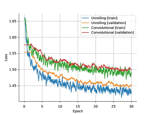
Figure 3.: Training and validation losses for the two models considered in this work. We see no hints of overfitting.fig:losses

The OTFs are computed from the autocorrelation of the generalized pupil function with a wavefront calculated with the KL expansion with 44 modes. The computation of the OTFs and the convolution of the estimated object and the instantaneous PSFs are computed using the Fast Fourier Transform (FFT). The training time for one epoch was $\sim$40 min for the case of the unrolling model and $\sim$28 min for the fully convolutional model. Note that, despite having more than 10 times more free parameters, the convolutional model is faster to evaluate. This is a consequence of the fact that computing the gradient of the loss function with respect to the wavefront coefficients for the unrolling model requires the computation of additional Fourier transforms.

We trained both models for 30 epochs. The training and validation losses are shown in Fig. fig:losses for both models. The validation loss saturates close to the end of the training, showing no signs of overfitting. Consequently, we choose the model parameters at the end of the training. The results show a slightly better training and validation loss for the unrolled model. We did not carry out any hyperparameter tuning because of computational reasons. We argue that the losses of both models can be made more similar and reach lower values after a suitable hyperparameter tuning phase.

The training of our model was performed on a single NVIDIA GeForce RTX 2080 Ti GPU. The neural network, as well as the computation of the loss function, was implemented and run using PyTorch 1.12 (Paszke et al., 2019). We used the Adam optimizer (Kingma and Ba, 2014) with a learning rate of $3\cdot 10^{-4}$.

At test time, the unoptimized correction of a full 1k$\times$1k image carried out in overlapping patches of 64$\times$64 takes only $\sim$8 seconds in a single 2080 Ti GPU for the unrolled model and $\sim$6 seconds for the convolutional model. This includes all I/O operations between the CPU and the GPU. In order to minimize the effect of the apodization while still being computationally efficient, the patches overlap 38 pixels, which is an area slightly larger than the chosen apodization window. The final image is constructed by mosaicking, built by averaging pixels from surrounding patches not taking into account the apodized regions. On average, our models can do the reconstruction of 64$\times$64 patches in $\sim$10 ms.

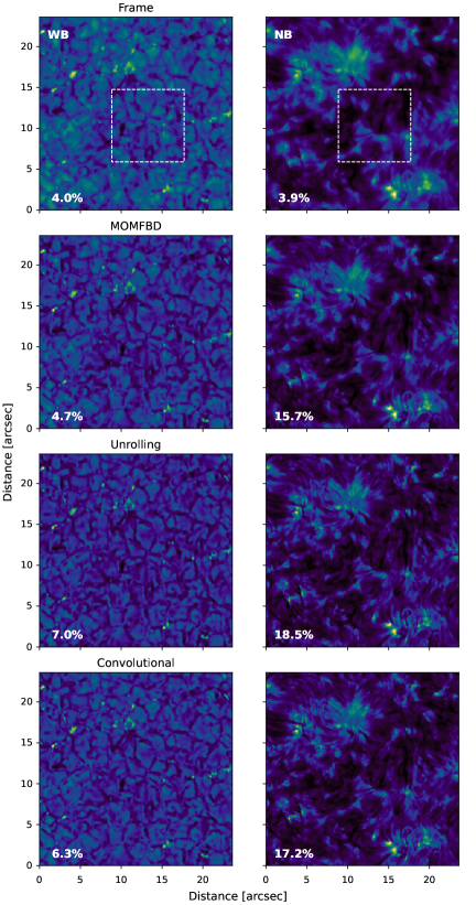
Figure 4.: Results of the restoration of an observation of the quiet Sun with CRISP in the Ca ii 8542 Å line taken on 01-Aug-19. The left column shows wideband images, while the right column displays the narrowband images corresponding to a wavelength displacement of +65 mÅ with respect to line center, which clearly shows conspicuous chromospheric structures. The contrast of the image shown in the image is computed on the displayed rectangle.fig:qs˙8542

5 Restoration

sec:results

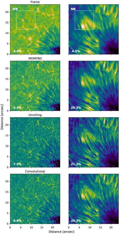
Figure 5.: Same as Fig. fig:qs_8542 but for the active region observed on 27-Jul-20. The narrowband image is chosen at +130 mÅ.fig:spot˙8542

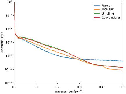
Figure 6.: Spatial azimuthal averaged power spectrum of the quiet Sun data shown in Fig. fig:qs_8542 for the wideband data.fig:qs˙power˙8542

5.1 CRISP

Once the models are trained, we validate our results by applying them to observations that were not part of the training set. We compare the results with the application of the classical MOMFBD code, which is performed in patches of 92$\times$92. Figures fig:qs_8542 and fig:spot_8542 show the results for CRISP observations in a quiet region and in an active region, respectively. Both observations were carried out in the Ca ii 8542 Å line. The figure shows the wideband images in the left column and the narrowband images in the right column. The top row shows the first frame of the burst, which gives an idea of the quality of the observations. The second row displays the results obtained with the classical MOMFBD code, while the remaining two rows show the results of our two models. In general, the restoring capabilities of our models are remarkable. A deeper analysis of some details individually, specially those appearing in the narrowband channel, suggests that our results produce a crispier image. It is well-known that the appearance of spatially correlated noise, inherent to image deconvolution, can lead to apparently crispier images. However, we do not see significant artifacts. It is true that the noise filter of the MOMFBD code has been refined with the passing years and we are simply using the recipe of Löfdahl and Scharmer (1994). Furthermore, we see no significant visual difference between the unrolled and the fully convolutional model. In order to make this comparison more quantitative, we have computed the contrast (rms intensity normalized to the average intensity) of the image in selected rectangles. We see that our neural approaches produce slightly larger contrasts than those of MOMFBD.

Similar conclusions can be extracted from the restoration of the active region observations displayed in Fig. fig:spot_8542 for the Ca ii 8542 Å line. Both the unrolled and the fully convolutional models produce slightly more crispier images than MOMFBD, where the superpenumbral filaments in the narrowband channel sampling the chromosphere show an improved contrast. The wideband images also display slightly more compact structures, with the dark penumbral filaments showing also more contrast.

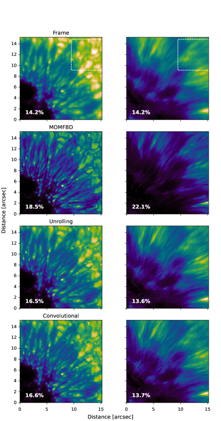
Figure 7.: Same as Fig. fig:qs_8542 but for the active region observed on 27-Jul-20 with the CHROMIS instrument in the Ca ii K line. The monochromatic wavelength is also placed at +65 mÅ from the line center.fig:spot˙3934

The visual impression suggested in the previous paragraphs is made more quantitative by inspecting the azimuthal average spatial power spectrum, as displayed in Fig. fig:qs_power_8542. The original frames contain a significant amount of noise in the large wavenumbers that is suitably filtered by the deconvolution process. A larger enhancement of the power appears in the range between wavenumbers 0.02 px^-1 and 0.3 px^-1. This is a consequence of the deconvolution recovering structures between 0.2” and 3”, which are destroyed in individual frames by the instantaneous PSFs. Our two neural models are almost equivalent and are able to extract a little more power in this range. This is the reason why the neural reconstructions looked crispier. On the contrary, the noise cancellation is similar between MOMFBD and our neural approaches. However, the strong reduction of power at large wavenumbers from MOMFBD suggests that their noise filter is performing slightly better than ours. This is not a fundamental limitation of the neural models and both models would perform similarly to MOMFBD in terms of noise cancellation if they eventually are part of the pipeline (Löfdahl et al., 2021).

5.2 CHROMIS

The results of applying the neural models to CHROMIS observations close to the core of the Ca ii K line are displayed in Fig. fig:spot_3934. The comparison of our results with those obtained with MOMFBD (using patches of size 88$\times$88) is rather unfair. The MOMFBD results are obtained taking into account the phase diversity channel, while ours does not use that channel. It is well-known (e.g., Löfdahl and Scharmer, 1994; van Noort, Rouppe van der Voort, and Löfdahl, 2005) that the addition of the defocused channel strongly constrains the results and produces much improved results, with the disadvantage of having to deal with more data and having a good alignment of the two channels. Even in this unfavorable case, our neural reconstructions produce excellent results although the inferred contrasts are smaller than those found with MOMFBD. Both neural approaches give comparable results. Of relevance, all structures in the umbra are recovered with contrast very similar to that of MOMFBD.

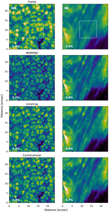
Figure 8.: Same as Fig. fig:qs_8542 but for HiFI for the observations on 28-Nov-22.fig:qs˙hifi

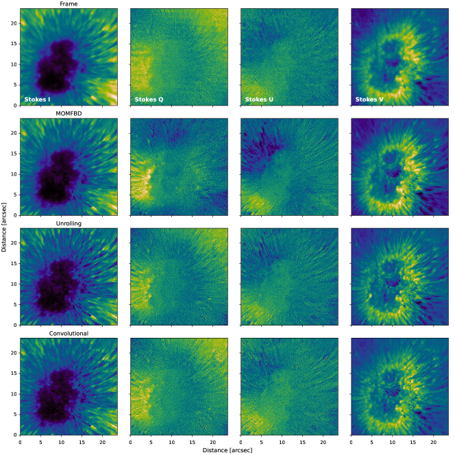
Figure 9.: Comparison of the Stokes parameter maps obtained after the polarimetric demodulation of the original CRISP frames, together with MOMFBD and our two neural models.fig:polarimetry

5.3 HiFI

As a final application of the neural reconstruction, we show in Fig. fig:qs_hifi a portion of a quiet-Sun region and their reconstructions observed with the HiFI instrument compared with that obtained with MOMFBD. The MOMFBD reconstruction was performed using 120 modes with 100 observed frames (note that this value is higher than the number of modes we use in our neural models), which seems to produce slightly over-reconstructed images, mainly visible on the wideband images. The neural reconstruction produces better-defined structures in these images, with filamentary features like those on locations $(x,y)=(1^{\prime\prime},17^{\prime\prime})$ or $(4^{\prime\prime},12^{\prime\prime})$ being much better defined in the neural restorations. This might be a consequence of the strong noise filter imposed in the MOMFBD reconstructions. The inferred contrasts are very similar in all cases, despite using a different number of modes in the MOMFBD reconstruction. Concerning the narrowband images, structures appear with similar quality in both neural reconstructions. One might argue that the MOMFBD reconstructions produce slightly more defined filaments in the upper right corner of the image. A few experiments carried out with this dataset shows that improvements in the image quality are marginal after 10-20 frames, and only noise is reduced.

5.4 Polarimetry

Although image reconstruction produces crispier images where the effect of the atmosphere has been reduced, it might affect the polarimetric properties of the observations. Following the strategy of van Noort and Rouppe van der Voort (2008), polarimetric information is recovered by modulating the measured intensity with the aid of a polarimeter. These measurements are then demodulated by inverting the modulation matrix. As a consequence, the Stokes parameters are recovered as linear combinations of the measured intensities. It is important to remember that each one of the measured modulation states is affected by slightly different atmospheric perturbations and they are all reconstructed independently, both in the classical MOMFBD code and in our neural approach. As a consequence, the addition and subtraction operations applied during the demodulation can produce artificial signals.

We use the calibrated modulation matrix for CRISP@SST to produce Stokes $I$ and Stokes $V$ monochromatic maps from the narrowband camera, which are displayed in Fig. fig:polarimetry. We see again images with a slightly better contrast with the neural approaches when compared with MOMFBD in Stokes $I$, similar to the results of Fig. fig:spot_8542. Concerning the polarimetric information, let us first look at Stokes $V$, which presents larger signals. The neural reconstruction produces more compact structures, especially on the unrolling model. This is clearly visible in the patch at position $(5^{\prime\prime},7^{\prime\prime})$, which corresponds to a penumbral grain clearly seen in Stokes $I$. The same happens for all the opposite polarity features (probably produced by strong Doppler motions) all around the penumbra, in consistency with what we observe in Stokes $I$. Concerning linear polarization, our neural models produce signals that are fundamentally the same signals as MOMFBD but weaker, more in accordance with the amplitudes seen in the original frames. Whether the MOMFBD data is affected in this case by deconvolution-induced crosstalk is something to be investigated in the future. The solution to this problem is difficult given the absence of a ground-truth solution. It is true, though, that our results display a little more spatially correlated noise. We anticipate that this can be alleviated with a slight improvement on the filter used in the Wiener estimation of the object. In general, the unrolling model produces slightly better results.

6 Conclusions

sec:conclusions We have presented two different neural models for the very fast restoration of solar images. The first one is based on algorithm unrolling, while the second one is an architectural improvement over the one published by Asensio Ramos and Olspert (2021). Both models are trained unsupervisedly with observations from the CRISP@SST, CHROMIS@SST and HiFI@GREGOR. Although the number of free parameters is more than an order of magnitude higher in the convolutional model, the gradient of the loss function needs to be computed in the unrolled model, so the evaluation time is similar in both models. In any case, they are several orders of magnitude faster in terms of computing time per anisoplanatic patch when compared with the classic MOMFBD code. Therefore, both approaches can be seen as strong candidates for a near real-time image restoration method for present and future observations.

Despite the promising results shown in this paper, there are still some points that need to be dealt with to fully exploit the capabilities of machine learning in solar image restoration. The first one is adding a phase diversity channel. This channel takes strictly simultaneous images but a known aberration (commonly a defocus) is added. This addition comes with the undesired effect of increasing the size of the observations, although improved reconstructions can be obtained (Löfdahl and Scharmer, 1994; van Noort, Rouppe van der Voort, and Löfdahl, 2005). Our training data does not contain this phase diversity channel, but both models can seamlessly use it. The images of this channel are assumed to have the same aberrations as those of the science camera, but with a known term added to Equation (eq:wavefront). The unrolled model can use a defocused channel by simply taking it into account during the computation of the gradient of the loss function. The convolutional model can deal with the phase diversity channel by stacking this image to the input of the Resnet18 encoder and computing the two OTFs (focused and defocused).

The second point is that, due to a lack of computing capabilities, we did a non-exhaustive search for architectures and training hyperparameters. An exhaustive search, with the aim of producing the most optimal architecture that leads to the best results, is left as work for the future.

The final point is how we can leverage machine learning to produce advances not only in terms of computing speed. In this sense, there are still a few ideas that have never been implemented and would improve image restoration. The first idea is adding time evolution during the reconstruction. Currently, every burst observed at a single scan position is deconvolved in isolation. As a consequence, once all bursts are deconvolved, the time coherence is a byproduct. This happens often for observations under good seeing conditions, but it is not the case when the seeing conditions are worse. Deconvolving all scan positions at once is a possibility, because one can introduce regularity constraints on the deconvolved images. A certain type of smoothness is foreseen in the reconstructed images because one does not expect sudden changes from one image to the next. This is simply a consequence of the limited sound speed in the solar atmosphere, which limits the amount of variability in the solar images obtained with a cadence of tens of seconds. The second idea is how to deal with spatially variant PSFs, a consequence of the small anisoplanatic patches in strong turbulence and/or large telescopes. The current overlap-add (OPA) approach or mosaicking (divide the image into overlapping small patches, which are then reconstructed and stitched back) is routinely used in solar physics (see, e.g., the excellent results of van Noort, Rouppe van der Voort, and Löfdahl, 2005). However, more precise approaches like the widespread method of Nagy and O’Leary (1998) and the recent space-variant OLA (Hirsch et al., 2010) methods can be used (see Denis et al., 2015, for a review). We are currently working on a deep learning approach to the spatially variant deconvolution that can simplify the deconvolution of whole images. When coupled together with the models described in this paper, we will be able to propose spatially variant deconvolution methods that can restore whole images in a single step.

Acknowledgments

The authors thank Michiel van Noort for invaluable advises on solar image restoration and Nigul Olspert for his work on the initial phases of this work. The authors acknowledge Sergio J. González Manrique, who participated in the GREGOR observing campaigns. The authors are also thankful to Andrea Diercke, the PI of the HiFI validation data, for allowing the use of the data. We also acknowledge Javier Trujillo Bueno for participating in the acquisition of the quiet-Sun data during our 2019 campaign at the SST. The Swedish 1-m Solar Telescope is operated on the island of La Palma by the Institute for Solar Physics of Stockholm University in the Spanish Observatorio del Roque de los Muchachos of the Instituto de Astrofísica de Canarias. The Institute for Solar Physics is supported by a grant for research infrastructures of national importance from the Swedish Research Council (registration number 2017-00625). The authors thankfully acknowledge the technical expertise and assistance provided by the Spanish Supercomputing Network (Red Española de Supercomputación), as well as the computer resources used: the La Palma Supercomputer, located at the Instituto de Astrofísica de Canarias. The 1.5-meter GREGOR solar telescope was built by a German consortium under the leadership of the Leibniz Institute for Solar Physics (KIS) in Freiburg with the Leibniz Institute for Astrophysics Potsdam (AIP), the Institute for Astrophysics Göttingen, and the Max Planck Institute for Solar System Research (MPS) in Göttingen as partners, and with contributions by the Instituto de Astrofísica de Canarias (IAC) and the Astronomical Institute of the Academy of Sciences of the Czech Republic (ASU).

Author Contribution

AAR proposed the two neural models, curated the training data, trained the models and analyzed the results. AAR made all figures and wrote the text. SEP observed and reduced the CRISP@SST and CHROMIS@SST data, also producing the MOMFBD restorations. CK observed and reduced the HiFI@GREGOR data, also producing the MOMFBD restorations. NO did some initial experiments on the convolutional model. SEP, CK and NO also contributed to the manuscript.

Funding

AAR acknowledges financial support from the Spanish Ministerio de Ciencia, Innovación y Universidades through project PGC2018-102108-B-I00 and FEDER funds. CK acknowledges funding from the European Union’s Horizon 2020 research and innovation programme under the Marie Skłodowska-Curie grant agreement No 895955. SEP acknowledges the funding received from the European Research Council (ERC) under the European Union’s Horizon 2020 research and innovation program (ERC Advanced grant agreement No. 742265).

Code Availability

The training and evaluation code is freely available in the following repository: https://github.com/aasensio/neural-MFBD. This repository also contains information on how to retrieve the training data.

Declarations

Conflict of interest

The authors declare that they have no conflicts of interest.

References

- Asensio Ramos and Olspert (2021) Asensio Ramos, A., Olspert, N.: 2021, Learning to do multiframe wavefront sensing unsupervised: Applications to blind deconvolution. A&A 646, A100.
- Asensio Ramos, de la Cruz Rodríguez, and Pastor Yabar (2018) Asensio Ramos, A., de la Cruz Rodríguez, J., Pastor Yabar, A.: 2018, Real-time, multiframe, blind deconvolution of solar images. A&A 620, A73.
- de la Cruz Rodríguez et al. (2013) de la Cruz Rodríguez, J., Rouppe van der Voort, L., Socas-Navarro, H., van Noort, M.: 2013, Physical properties of a sunspot chromosphere with umbral flashes. A&A 556, A115.
- Denis et al. (2015) Denis, L., Thiébaut, É., Soulez, F., Becker, J.-M., Mourya, R.: 2015, Fast Approximations of Shift-Variant Blur. International Journal of Computer Vision 115, pp 253.
- Denker et al. (2023) Denker, C.J., Verma, M., Wiśniewska, A., Kamlah, R., Kontogiannis, I., Dineva, E., Rendtel, J., Bauer, S.-M., Dionies, M., Önel, H., Woche, M., Kuckein, C., Seelemann, T., Pal, P.S.: 2023, Improved High-resolution Fast Imager. Journal of Astronomical Telescopes, Instruments, and Systems 9, 015001.
- Gonsalves and Chidlaw (1979) Gonsalves, R.A., Chidlaw, R.: 1979, Wavefront sensing by phase retrieval. In: A. G. Tescher (ed.) Society of Photo-Optical Instrumentation Engineers (SPIE) Conference Series, Presented at the Society of Photo-Optical Instrumentation Engineers (SPIE) Conference 207, 32.
- Gregor and LeCun (2010) Gregor, K., LeCun, Y.: 2010, Learning Fast Approximations of Sparse Coding. In: Proceedings of the 27th International Conference on International Conference on Machine Learning, ICML’10, Omnipress, Madison, WI, USA, 399–406.
- He et al. (2015) He, K., Zhang, X., Ren, S., Sun, J.: 2015, Deep Residual Learning for Image Recognition. CoRR abs/1512.03385. http://arxiv.org/abs/1512.03385.
- Hendrycks and Gimpel (2016) Hendrycks, D., Gimpel, K.: 2016, Gaussian Error Linear Units (GELUs). arXiv e-prints, arXiv:1606.08415.
- Hirsch et al. (2010) Hirsch, M., Sra, S., Schölkopf, B., Harmeling, S.: 2010, Efficient Filter Flow for Space-Variant Multiframe Blind Deconvolution. In: Proceedings of the 23rd IEEE Conference on Computer Vision and Pattern Recognition, IEEE, Piscataway, NJ, USA, 607. Max-Planck-Gesellschaft.
- Kingma and Ba (2014) Kingma, D.P., Ba, J.: 2014, Adam: A Method for Stochastic Optimization. arXiv e-prints, arXiv:1412.6980.
- Kleint et al. (2020) Kleint, L., Berkefeld, T., Esteves, M., Sonner, T., Volkmer, R., Gerber, K., Krämer, F., Grassin, O., Berdyugina, S.: 2020, GREGOR: Optics redesign and updates from 2018-2020. A&A 641, A27.
- Kuckein et al. (2017) Kuckein, C., Denker, C., Verma, M., Balthasar, H., González Manrique, S.J., Louis, R.E., Diercke, A.: 2017, sTools - a data reduction pipeline for the GREGOR Fabry-Pérot Interferometer and the High-resolution Fast Imager at the GREGOR solar telescope. In: Vargas Domínguez, S., Kosovichev, A.G., Antolin, P., Harra, L. (eds.) Fine Structure and Dynamics of the Solar Atmosphere 327, 20.
- Labeyrie (1970) Labeyrie, A.: 1970, Attainment of Diffraction Limited Resolution in Large Telescopes by Fourier Analysing Speckle Patterns in Star Images. Astron. Astrophys. 6, 85.
- Löfdahl and Scharmer (1994) Löfdahl, M.G., Scharmer, G.B.: 1994, Wavefront sensing and image restoration from focused and defocused solar images. Astron. Astrophys.s 107, 243.
- Löfdahl et al. (1998) Löfdahl, M.G., Berger, T.E., Shine, R.S., Title, A.M.: 1998, Preparation of a Dual Wavelength Sequence of High-Resolution Solar Photospheric Images Using Phase Diversity. Astrophys. J. 495, 965.
- Löfdahl et al. (2002) Löfdahl, M.G., Bones, P.J., Fiddy, M.A., Millane, R.P.: 2002, Multi-frame blind deconvolution with linear equality constraints. In: Image Reconstruction from Incomplete Data 4792, 146.
- Löfdahl et al. (2021) Löfdahl, M.G., Hillberg, T., de la Cruz Rodríguez, J., Vissers, G., Andriienko, O., Scharmer, G.B., Haugan, S.V.H., Fredvik, T.: 2021, SSTRED: Data- and metadata-processing pipeline for CHROMIS and CRISP. A&A 653, A68.
- Monga, Li, and Eldar (2021) Monga, V., Li, Y., Eldar, Y.C.: 2021, Algorithm Unrolling: Interpretable, Efficient Deep Learning for Signal and Image Processing. IEEE Signal Processing Magazine 38, 18.
- Nagy and O’Leary (1998) Nagy, J.G., O’Leary, D.P.: 1998, Restoring Images Degraded by Spatially Variant Blur. SIAM Journal on Scientific Computing 19, 1063.
- Noll (1976) Noll, R.J.: 1976, Zernike polynomials and atmospheric turbulence. Journal of the Optical Society of America 66, 207.
- Oscoz et al. (2008) Oscoz, A., Rebolo, R., López, R., Pérez-Garrido, A., Pérez, J.A., Hildebrandt, S., Rodríguez, L.F., Piqueras, J.J., Villó, I., González, J.M., Barrena, R., Gómez, G., García-Hernández, D.A., Montañés, P., Rosenberg, A., Cadavid, E., Calcines, A., Díaz-Sánchez, A., Kohley, R., Martín, Y., Peñate, J., Sánchez, V.: 2008, FastCam: a new lucky imaging instrument for medium-sized telescopes, Society of Photo-Optical Instrumentation Engineers (SPIE) Conference Series 7014, 701447.
- Paszke et al. (2019) Paszke, A., Gross, S., Massa, F., Lerer, A., Bradbury, J., Chanan, G., Killeen, T., Lin, Z., Gimelshein, N., Antiga, L., Desmaison, A., Kopf, A., Yang, E., DeVito, Z., Raison, M., Tejani, A., Chilamkurthy, S., Steiner, B., Fang, L., Bai, J., Chintala, S.: 2019, PyTorch: An Imperative Style, High-Performance Deep Learning Library. In: Wallach, H., Larochelle, H., Beygelzimer, A., d’é-Buc, F., Fox, E., Garnett, R. (eds.) Advances in Neural Information Processing Systems 32, Curran Associates, Inc., 8024.
- Paxman, Schulz, and Fienup (1992) Paxman, R.G., Schulz, T.J., Fienup, J.R.: 1992, Joint estimation of object and aberrations by using phase diversity. Journal of the Optical Society of America A 9, 1072.
- Scharmer (2017) Scharmer, G.: 2017, SST/CHROMIS: a new window to the solar chromosphere. In: SOLARNET IV: The Physics of the Sun from the Interior to the Outer Atmosphere, 85.
- Scharmer (2006) Scharmer, G.B.: 2006, Comments on the optimization of high resolution Fabry-Pérot filtergraphs. A&A 447, 1111.
- Scharmer et al. (2003) Scharmer, G.B., Bjelksjo, K., Korhonen, T.K., Lindberg, B., Petterson, B.: 2003, The 1-meter Swedish solar telescope. In: Keil, S.L., Avakyan, S.V. (eds.) Innovative Telescopes and Instrumentation for Solar Astrophysics, Society of Photo-Optical Instrumentation Engineers (SPIE) Conference Series 4853, 341.
- Scharmer et al. (2008) Scharmer, G.B., Narayan, G., Hillberg, T., de la Cruz Rodriguez, J., Löfdahl, M.G., Kiselman, D., Sütterlin, P., van Noort, M., Lagg, A.: 2008, CRISP Spectropolarimetric Imaging of Penumbral Fine Structure. ApJ 689, L69.
- Schmidt et al. (2012) Schmidt, W., von der Lühe, O., Volkmer, R., Denker, C., Solanki, S.K., Balthasar, H., Bello Gonzalez, N., Berkefeld, T., Collados, M., Fischer, A., Halbgewachs, C., Heidecke, F., Hofmann, A., Kneer, F., Lagg, A., Nicklas, H., Popow, E., Puschmann, K.G., Schmidt, D., Sigwarth, M., Sobotka, M., Soltau, D., Staude, J., Strassmeier, K.G., Waldmann , T.A.: 2012, The 1.5 meter solar telescope GREGOR. Astronomische Nachrichten 333, 796.
- van Noort, Rouppe van der Voort, and Löfdahl (2005) van Noort, M., Rouppe van der Voort, L., Löfdahl, M.G.: 2005, Solar Image Restoration By Use Of Multi-frame Blind De-convolution With Multiple Objects And Phase Diversity. Sol. Phys. 228, 191.
- van Noort and Rouppe van der Voort (2008) van Noort, M.J., Rouppe van der Voort, L.H.M.: 2008, Stokes imaging polarimetry using image restoration at the Swedish 1-m solar telescope. A&A 489, 429.
- von der Lühe (1993) von der Lühe, O.: 1993, Speckle imaging of solar small scale structure. I - Methods. Astron. Astrophys. 268, 374.