Learning Latent Dynamics via Invariant Decomposition and (Spatio-)Temporal Transformers

Abstract

We propose a method for learning dynamical systems from high-dimensional empirical data that combines variational autoencoders and (spatio-)temporal attention within a framework designed to enforce certain scientifically-motivated invariances. We focus on the setting in which data are available from multiple different instances of a system whose underlying dynamical model is entirely unknown at the outset. The approach rests on a separation into an instance-specific encoding (capturing initial conditions, constants etc.) and a latent dynamics model that is itself universal across all instances/realizations of the system. The separation is achieved in an automated, data-driven manner and only empirical data are required as inputs to the model. The approach allows effective inference of system behaviour at any continuous time but does not require an explicit neural ODE formulation, which makes it efficient and highly scalable. We study behaviour through simple theoretical analyses and extensive experiments on synthetic and real-world datasets. The latter investigate learning the dynamics of complex systems based on finite data and show that the proposed approach can outperform state-of-the-art neural-dynamical models. We study also more general inductive bias in the context of transfer to data obtained under entirely novel system interventions. Overall, our results provide a promising new framework for efficiently learning dynamical models from heterogeneous data with potential applications in a wide range of fields including physics, medicine, biology and engineering.

1 Introduction

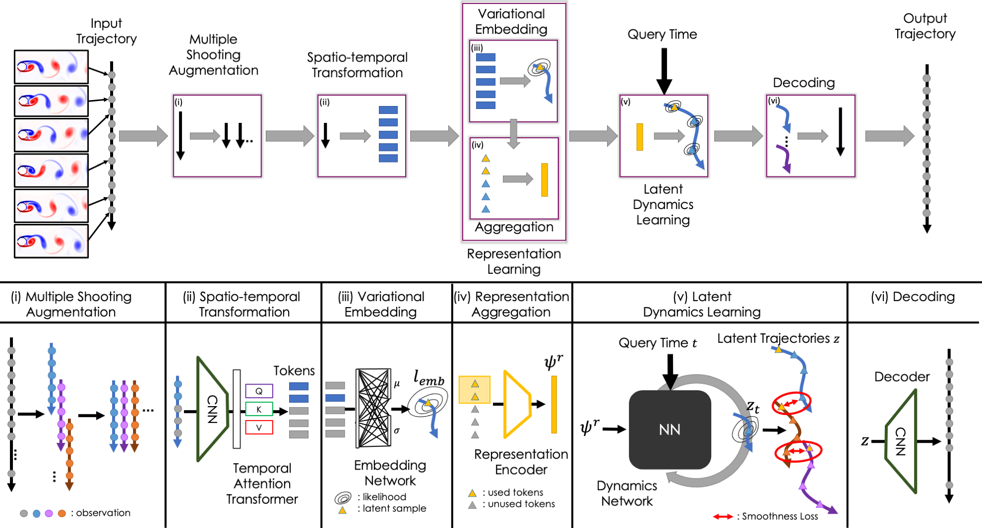
Figure 1: Architecture: Learning of Latent Dynamics via Invariant Decomposition (LaDID). Top half: general flow chart of the compute steps (i)-(v) of LaDID; lower half: more detailed representation of the compute steps. A set of high-dimensional snapshots of a system on a regular or irregular time-grid serves as the empirical input to LaDID. The trajectory is split into subpatches using Multiple Shooting Augmentation (i). The first time-points of each subpatch are used to compute a subtrajectory representation: features of the selected snapshots are re-weighted wrt time and spatial location (ii), transformed to low-dimensional variational embedding (iii), and aggregated into one trajectory representation $\psi_{r}$ (iv). During inference, the latent dynamical model is conditioned on the specific representation $\psi_{r}$. Prediction is possible at any continuous time by querying the latent state of any time point of interest (v). Latent subtrajectories are sewn together by a smoothness loss. Finally, the entire latent trajectory is decoded to the observation space (vi).

Dynamical models are central to our ability to understand and predict natural systems. For many systems of interest in fields like biology, medicine and engineering, high-dimensional observations can reasonably be thought of as obtained via dynamics operating in a lower dimensional space and this assumption (related to the manifold hypothesis [15]) is a common one in many settings. Machine learning (ML) approaches for learning dynamical systems have been an important area of recent research, including in particular neural ordinary differential equations [9] and a wider class of related neural-dynamical models ([46, 16, 12, 10, 8, 27]). These models define layers as differential equations and in that sense incorporate an informative (and often appropriate) inductive bias for physical systems.

In this paper, we propose a new framework for learning latent dynamics from observed data. Our approach, called “Latent Dynamics via Invariant Decomposition” (LaDID), combines variational autoencoders and spatio-temporal attention within a learning framework motivated by certain scientifically-motivated invariances. The LaDID framework exploits these invariances and provides model output at any continuous time but does not require an explicit ODE formulation (details below). Although the focus of this paper is primarily on methodology, the research we present is motivated by real-world applications, particularly in the fields of biomedicine and health. In these domains, it is often the case that explicit dynamical models are not initially accessible; however we expect that the unknown dynamical models should nevertheless satisfy the very general invariances outlined below (see also Discussion).

The methods we propose build on two observations concerning classical scientific models:

• First, the notion that every output from a class of scientific systems should be explainable via a single model despite differences between individual instances within a class. In this sense, the model is considered universal, even if there are large differences in observed data across instances. For instance, in the case of mechanical systems, one set of equations can effectively describe diverse instances (e.g. by accounting for dissimilar initial conditions or constants). This is intriguing from an ML perspective since the distribution of data can vary greatly between instances, leading to significant shifts.

• Second, instance/realization-specific factors (such as initial conditions or constants) tend to remain unchanged throughout the entire duration of a given realization. In this regard, these factors exhibit time invariance, as they maintain their values consistently over time.

Our approach and the derived transformer-based architecture builds directly on these notions of invariance. We describe the network in detail below, but in brief the set-up is as follows: From an available trajectory – thought of as representing a specific instance/realization $r$ of a more general model class $\mathcal{M}$ – we learn an encoding $\psi^{r}$ of the realization-specific information. This is intended to implicitly capture information (such as initial conditions or constants) that are specific to the instance or realization $r$, but the information should remain valid for all times within a realization/instance; hence the encoding has a superscript indicating the realization but no time index. This encoding $\psi^{r}$ is treated as an input to a “universal” model $f$ to enable prediction of system output at any time $t$. The model $f$ itself is learned across multiple realizations $r$ of the system defined by the model class but the same function is always used for prediction (for the system $\mathcal{M}$). In other words, $f$ is intended to be universal (across all queries concerning the system $\mathcal{M}$) with realization-specific information provided only by the input $\psi^{r}$. We argue that under certain conditions, this decomposition into realisation-specific (RS) and realization-invariant (RI) information allows for definition of a simple and convenient learning framework. We propose a deep neural architecture for this purpose, showing how learning of universal latent dynamics and realization-specific information can be done jointly, in an end-to-end manner. This enables prediction of system behaviour at any continuous time $t$, for any realization $r$ (for which minimal data are available).

We empirically validate our proposed method on spatio-temporal systems with dynamics governed by ordinary or partial differential equations. These systems are ubiquitous in nature and include physical phenomena in rigid body motion, fluid dynamics and turbulent flows, electromagnetism and molecular dynamics. Our work is related to a large body of previous work on neural learning of dynamical models, which we discuss in detail below. A key distinction of our approach is that by leveraging the framework outlined above, we do not require an explicit neural ODE (NODE) at all; rather we can carry out learning within a simple, broadly supervised framework that, as we show, can in fact outperform existing neural-dynamical models over a range of challenging tasks on both regular and irregular time grids.

Thus, the main contributions of this paper are:

• We present a novel framework, and associated transformer-based network, for the separation and learning of realization-specific information and (realization-invariant) latent dynamical systems.

• We systematically study performance on short- and longer-horizon prediction of a wide range of complex temporal and spatio-temporal problems, comparing against a range of state-of-the-art neural-dynamical methods.

• We study the challenging case of transfer to data obtained under entirely novel system interventions via a few-shot learning approach.

The remainder of the paper is organized as follows. We first introduce the problem statement, basic conceptual ideas and assumptions and the proposed architecture. We then present empirical work, spanning a wide range of different, challenging dynamical systems. We close with comments on limitations and future directions.

2 Related Work

We begin with a short survey of the rich body of recent work on ML-based approaches aimed at learning dynamical models from data. [6, 25] access Koopman theory to learn coefficients of a finite set of non-linear functions to approximate the observed dynamics. Other approaches [11, 33, 19, 17, 47, 1] induce Hamiltonian and Lagrangian priors into neural networks exploiting the reformulations of Newton’s equations of motion in energy-conservative dynamics. This inductive bias allows for accurate predictions over a significantly wider time-horizon but involves strong assumptions. Purely data-driven ML approaches have attracted much recent attention and have shown strong performance in many areas. [22] learn a data-driven approximation of a dynamical system via a Gaussian Processes and [30] formulates a new neural operator by parameterizing the integral kernel directly in Fourier space to allow zero-shot prediction for an entire family of PDEs.

In a recent line of research, the ability of NNs to approximate arbitrary functions has been exploited for unknown dynamical models, with connections drawn between deep architectures and numerical solvers for ODEs, PDEs and SDEs [9, 14, 32, 43, 20, 41]. This has given rise to new algorithms rooted in neural differential equations that have been shown to provide improved modeling of a variety of dynamical systems relative to standard recurrent neural networks (RNNs) and their variants. Improvements for neural ODEs have been proposed: [13] put forward a simple augmentation to the state space to broaden the range of dynamical systems that can be learned; [26] propose neural controlled differential equations; [37] incorporate concepts of rough theory to extend applicability to trajectories spanning thousands of steps, and [24] explore extensions to account for interrupting stochastic events. The work of [42] combines an autoregressive RNN updated at irregularly sampled time points with an NODE model that computes inter-observation states in continuous time. Their work also includes a variational autoencoder (VAE) extension to uncover latent processes based on high-dimensional observations. In related work, [44] proposed a VAE for sequential data with a latent space governed by a continuous-time probabilistic ODE. [34] transferred the concept of multiple shooting to solve differential equations to the conceptual space of NODEs and [23] extended this concept to sparse Bayesian multiple shooting, with both works evaluating latent NODEs.

Our approach is inspired by this body of work in that we also use neural networks to learn latent dynamical models. However, two key differences are as follows. First, our models are specifically designed to exploit certain invariances that are important in classical scientific models (as detailed below). From this point of view, we leverage a particular kind of scientifically-motivated inductive bias from the outset. Second, exploiting these invariances allows us to eschew explicit neural ODEs altogether, providing an arguably simpler, transformer-based scheme that can be trained in a straightforward fashion, but that, as we show, is effective across a range of dynamical problems and that can even be leveraged for few-shot learning to generalize to nontrivial system interventions.

3 Methods

We first provide a high-level problem statement. We then consider some simple arguments to support the idea that a relatively straightforward learning framework can be applied in this setting. These simple but general arguments are intended to shed light on the learning problem and provide conceptual background. We then put forward a specific architecture to permit learning in practice, i.e. a concrete learning framework that we implement and study empirically.

3.1 Problem statement

We focus on settings in which available training data corresponds to multiple instances or realizations of a system class of interest. We seek to learn a model that allows prediction of the system at any continuous time for any realization/instance (this set-up is common in many areas of science, engineering and medicine, and we study several specific examples in results below). Let $X_{r,j,t}\!\in\!\mathbb{R}^{p}$ denote observed data for realization $r$ at time $t$, with $j$ indexing the dimension. In the training phase, we assume that for each of $R$ different realizations we have access to an observed trajectory of $T$ time points. We need to know the sampling times themselves, but these need not be evenly spaced. Hence, the input $X$ is of size $R{\times}p{\times}T$. We treat the $p$-dimensional observations as arising from an underlying process $f^{*}$ operating in $q{<}p$ dimensions coupled with a time-independent observation process $g:\mathbb{R}^{q}\rightarrow\mathbb{R}^{p}$. Our goal is to learn a latent dynamical model $f$ that allows prediction of $X_{r,j,t}$ at any time $t$ and for any realization $r$. For realizations that were not represented in the training data at all, we assume availability of some data specific to the realization at inference-time.

3.2 From invariances to a simple learning framework

In this Section, we consider an abstract version of the problem of interest, aimed at clarifying the specific invariances that will be needed and gaining understanding of how learning can be conveniently performed in this setting. The notation in this Section is self-contained but (in the interests of expositional clarity) differs from the following Sections providing architectural and implementation details.

General formulation. Consider an entirely general system $f$ which may be deterministic or stochastic (with all random components absorbed for convenience into $f$). We are interested in settings in which some aspects of the model are realisation-specific (RS) while others remain realisation-invariant (RI). Let

$$x^{r}_{t}{=}f(t;\Theta_{r}),\,x^{r}_{t}{\in}\mathbb{R}^{p}$$

denote the fully general model. Here, $\Theta_{r}$ is the complete parameter needed to specify the time-evolution, including both RS and RI parts. To make the separation clear, we write the two parts separately as $x^{r}_{t}{=}f(t;\theta_{r},\theta)$, where $\theta_{r}$, $\theta$ are respectively the RS and RI parameters (together comprising $\Theta_{r}$).

We call this a generalized initial condition formulation, as it generalizes the idea of an initial condition in ODEs. In the case of an ODE, the initial conditions and relevant constants are the information needed, in addition to the model equations themselves, to fully specify the time evolution of any specific instance/realization of the model. In our terms, if a problem/dataset has one model but many such “initial conditions” (more precisely this can be any RS aspect, including constants), then the model itself is RI, while the initial conditions/constants are the RS part. Note that although we do not assume any specific knowledge about the system (other than the motivating invariances), we do assume that we can at the outset block datasets into instances arising from a shared system (whose details are entirely unknown); in this paper we do not consider the task of learning the system classification itself from data.

Fully observed case. In the model $f$ above, the true parameter $\Theta_{r}=(\theta_{r},\theta)$ comprises RS and RI parts. We now provide conditions under which learning of the system state at any continuous time $t$ is possible without explicit knowledge of either the model $f$ or the true parameter $\Theta_{r}$. We start with the simplest case of fully observed data (i.e. no latent dynamics) and then consider the latent case. The idea is to work from a candidate encoding $\hat{\theta}_{r}$ of the RS information. In practice this would be the output of a neural network (NN) based on initial data from a realization $r$ and itself learned end-to-end jointly with other model components; see subsequent Sections for architectural and implementation details. The encoding $\hat{\theta}_{r}$ is intended to be a representation of RS information that, as we will see below, under certain assumptions can be combined with a universal model to allow effective prediction.

Specifically, we assume that the encoding $\hat{\theta}_{r}$, while possibly incorrect (i.e. such that $\hat{\theta}_{r}{\neq}\theta_{r}$) satisfies the property

$$\exists m,\exists\theta_{m}:\theta_{r}{=}m(\hat{\theta}_{r};\theta,\theta_{m}),$$

where $m$ is a function that “corrects” $\hat{\theta}_{r}$ to give the correct RS parameter. Note that the correction function $m$ can potentially use the RI parameter of the system and possibly additional parameters $\theta_{m}$. This essentially demands that while the encoding $\hat{\theta}_{r}$ might be very different from the true value (and may even diverge from it in a complicated way that depends on unknown system parameters), there exists an RI transformation that recovers the true RS parameter from it, and in this sense the encoding contains all RS information. We call this the sufficient encoding assumption (SEA). Note that the function $m$ has an oracle-like property in that it may depend on the true RI parameter $\theta$ and we will not have access to $m$ in practice.

We would like to learn a mapping that takes as input the RS encoding $\hat{\theta}_{r}$ and query time point $t$ and yields the correct system output (for any realization and any time). That is, the input to the mapping would be the pair $(t,\hat{\theta}_{r})$ and the output intended to predict $x_{t}^{r}$. To this end, consider the candidate prediction

$$\hat{x}_{t}^{r}{=}f(t;m(\hat{\theta}_{r};\theta,\theta_{m}),\theta),$$

and observe that we can always write the RHS as $h(t,\hat{\theta}_{r};\Xi)$ where $\Xi=(\theta,\theta_{m})$ is a RI parameter and $h$ is a function (obtained by combining $f$ and $m$ as above). This latter formulation emphasizes the fact that the RHS is in fact a function (here, $h$) of only the inputs $(t,\hat{\theta}_{r})$, and therefore potentially learnable from training pairs. Note that the parameters of $h$ are entirely RI and hence the only RS information is carried by the encoding $\hat{\theta}_{r}$. It is easy to see that under SEA this construction provides the correct output since we can write the RHS as $f(t;m(\hat{\theta}_{r};\theta,\theta_{m}),\theta)=f(t;\theta_{r},\theta)=x_{t}^{r}$. Thus, combining encoding $\hat{\theta}_{r}$ and function $h$ allows prediction of the time evolution of any realisation. In other words, even if the RS encoding is distant from the true RS parameter, under SEA there exists a RI function that can correct it, and we can therefore seek to train a NN aimed at learning a function $h$ which combines these RI elements to provide the desired mapping.

Latent dynamics. In line with the manifold hypothesis, consider now dynamics at the level of latent variables $z\in\mathbb{R}^{q}$ and again consider a model with RS and RI parts but at the level of the latents, i.e. $z^{r}_{t}=f(t,\hat{\theta}_{r};\theta_{r},\theta)$. We assume that the observables are given by (an unknown) function of the hidden state $z$. We first consider the case in which the latent-to-observed mapping is RI, and then the more general case of a RS mapping.

Case I: RI mapping. Assume the observable is given as $x^{r}_{t}=g(z^{r}_{t};\theta_{g})$, where $g:\mathbb{R}^{q}\rightarrow\mathbb{R}^{p}$ is the (true) observation process and $\theta_{g}$ is an RI parameter. Further, assume that we have an estimate $\hat{\theta}_{r}$ of the RS encoding that satisfies the sufficient encoding assumption (SEA). In a similar fashion, assume we have an estimate $\hat{\theta}_{g}$, which may be incorrect (in the sense of $\hat{\theta}_{g}\neq\theta_{g}$) but that satisfies: $\exists m_{g},\exists\theta_{m_{g}}:\theta_{g}=m_{g}(\hat{\theta}_{g};\theta,\theta_{m_{g}})$. That is, $\hat{\theta}_{g}$ admits an RI correction. As above, the correction is oracle-like and may potentially depend on true RS parameters. Note also that subject to the existence of a correction the estimate (and implied mapping) may be potentially arbitrarily incorrect. In analogy to SEA, we call this the sufficient mapping assumption (SMA).

Now, consider training of a NN, with training (input, output) pairs of the form $\{(t,\hat{\theta}_{r}),x_{t}^{r}\}_{(t,r)\in Train}$. We want to understand whether supervised learning of a universal model to predict output for arbitrary queries $(t,r)$ is possible. This is not obvious, since we now have training data only at the level of the observables, but the actual dynamics operate at the level of latents. Consider the following function $h_{SMA}$:

$$h_{SMA}(t,\hat{\theta}_{r};\Xi)=g(f(t;m(\hat{\theta}_{r};\theta,\theta_{m});m_{g}(\hat{\theta}_{g};\theta,\theta_{m_{g}}))$$

where $\Xi=(\theta,\theta_{m},\theta_{m_{g}})$ is an RI parameter.

Under SEA and SMA it is easy to see that $h_{SMA}$ provides the correct output, since:

$$h_{SMA}(t,\hat{\theta}_{r};\Xi) =g(f(t;m(\hat{\theta}_{r};\theta,\theta_{m});m_{g}(\hat{\theta}_{g};\theta,\theta_{m_{g}}))$$

$$=g(f(t;\theta_{r},\theta);\theta_{g})$$

$$=g(z^{r}_{t};\theta_{g})$$

$$=x^{r}_{t}$$

That is, under SEA and SMA there exists a function of $t$ and $\hat{\theta}_{r}$ that provides the correct output and that is universal in the sense that (i) the same function applies to any query $(t,r)$ and (ii) its parameter is itself RI and hence the same for all realizations.

Case II: RS mapping. Suppose now the mapping is RS, with the model specification as above but with the observation step $x^{r}_{t}=g(z^{r}_{t};\theta^{r}_{g})$, where $\theta^{r}_{g}$ is an RS parameter. This means that the latent-observable relationship is itself non-constant and instead varies between realizations.

Assume we have a candidate estimate $\hat{\theta}^{r}_{g}$ which may be incorrect in the sense of $\hat{\theta}^{r}_{g}\neq\theta^{r}_{g}$ but that satisfies: $\exists m_{g},\exists\theta_{m_{g}}:\theta_{g}=m_{g}(\hat{\theta}^{r}_{g};\theta,\theta_{m_{g}})$. In analogy to SMA, we call this the realization-specific sufficient mapping assumption or RS-SMA. Now to create training sets, we extend the formulation to require input triples, as: $\{(t,\hat{\theta}_{r},\hat{\theta}_{g}^{r}),x_{t}^{r}\}_{(t,r)\in Train}$. In a similar spirit to the RS encoding above, $\hat{\theta}_{g}^{r}$ in the input triples may be incorrect, but only needs to satisfy RS-SMA. As in Case I, we have training data only at the level of observables (not latents) but want to understand whether supervised learning of a model to predict output for arbitrary queries $(t,r)$ is possible. Consider the function $h_{RS-SMA}$:

$$h_{RS-SMA}(t,\hat{\theta}_{r},\hat{\theta}_{g}^{r};\Xi)=g(f(t;m(\hat{\theta}_{r};\theta,\theta_{m}),\theta);m_{g}(\hat{\theta}_{g}^{r};\theta,\theta_{m_{g}}))$$

where $\Xi=(\theta,\theta_{m},\theta_{m_{g}})$ is an RI parameter. In a similar manner to Case I, it is easy to see that $h_{RS-SMA}$ provides the correct output under SEA and RS-SMA, since:

$$h_{RS-SMA}(t,\hat{\theta}_{r},\hat{\theta}_{g}^{r};\Xi) =g(f(t;m(\hat{\theta}_{r};\theta,\theta_{m}),\theta);m_{g}(\hat{\theta}_{g}^{r};\theta,\theta_{m_{g}}))$$

$$=g(f(t;\theta_{r},\theta);\hat{\theta}_{g}^{r})$$

$$=g(z^{r}_{t};\hat{\theta}_{g}^{r})$$

$$=x^{r}_{t}$$

The foregoing arguments are based on an abstract view of the task at hand and show that under the assumptions above, there exist universal mappings from the available inputs to the desired outputs whose parameters are themselves RI. As a result, subject to the assumptions above, it may be possible to learn suitable mapping functions from data (without requiring prior access to the various components). We now put forward a specific architecture aimed at learning such a mapping in practice.

3.3 Neural architecture

In this Section we provide details on the NN architecture and implementation. Additional notation is required to clarify the relevant details; the exposition below is self-contained and intended to be concise, however the notation differs from that in Section 3.2 above. We note also that the architecture introduced in this Section is only one approach by which to instantiate the general ideas above.

We seek to learn a model able to predict future observations $x_{t:T}^{r}$ based on a sequence of $k$ past time points $x_{t-k:t-1}^{r}$. To this end, we use a variational autoencoder (VAE) [28, 40] within our model. From a high-level point of view, it consists of an encoder network that learns to embed a set of observations of different realisations $X_{1:T}^{r}$ to a low-dimensional embedding $z_{1:T}^{r}\sim q_{\Phi_{L}}(\cdot|X_{1:T}^{r})$ and $\Phi_{L}$ being the parameter set of the transformation to the latent space. The dynamics are modelled in this inferred state space stochastically. Finally, a decoder network maps the position coordinates in the state space back to the image/observation space $p(X_{1:T}^{r})=\mathcal{D}_{\phi_{dec}}(z_{1:T}^{r})$.

In more details, the encoder is a collection of three NNs. First, features from the input observations $x_{t-k:t-1}^{r}$ are extracted using a convolutional neural network (CNN) parameterized by $\phi_{enc}$ shared across all representations and patches (see multiple shooting augmentation below). Our CNN encoder transforms the sequence of input observations to a sequence of feature vectors, $z^{(enc),r}_{t-k:T}{=}f_{\phi_{enc}}(x^{r}_{t-k:T})$. Then, we compute the trajectory representation and the latent embedding as follows. Each input patch is split into two disjoint sets by time. The first $k$ data points $\mathcal{M}_{R}{=}\{z^{(enc),r}_{t-k:t}\}$ are used to compute a trajectory specific representation distribution $\psi^{r}{\sim}q_{\Phi_{R}}(x_{t-k:t-1}^{r})=\mathcal{N}(\mu_{r},\sigma_{r})$ and $\mu_{r},\sigma_{r}{=}f_{\Phi_{R}}(z^{(enc),r}_{t-k:t})$. In cases of irregularly sampled trajectories, we use a time threshold $\tau$ to define the representation set, $\mathcal{M}_{R}{=}\{z^{(enc),r}_{t_{i}}\},\,t_{i}{\in}\{t{<}\tau\}$. We model $f_{\phi_{R}}$ as a transformer network with temporal attention. In other words, we consider the sequence feature vectors $z^{(enc),r}_{t-k:t}$ as an time-ordered sequence of tokens and transform each token according to the temporal distance to the other tokens. The trajectory representation $\psi^{r}$ is the mean-aggregation of the temporally transformed representation tokens. With initial density given by the encoder networks $q_{\Phi_{L}}(z_{t}|x^{r}_{t-k:T},\psi^{r})$, the density for all queried latent points (on a continuous time grid) can be predicted by $z_{t_{q}}^{r}{\sim}\mathcal{N}(\mu_{t_{q}}^{r},\sigma_{t_{q}}^{r})$ with $\mu_{t_{q}}^{r},\sigma_{t_{q}}^{r}{=}f_{\phi_{dyn}}(t_{q},z_{t},\psi^{r})$. Note that this approach allows for latent state predictions at any time since the learned dynamics module $f_{\phi_{dyn}}$ is continuous in time and our variational model utilizes encoders only for obtaining the initial latent distribution. We also make use of the reparameterization trick to tackle uncertanties in both the latent states and in the trajectory representations [28]. Finally, the decoder maps the latent state to the output. In summary, our variational model is defined as follows:

Encoder $\mu_{r},\sigma_{r}=f_{\phi_{R}}((f_{\phi{enc}}(x^{r}_{t-k:t})$ Reparameterization $\psi^{r}\sim q_{\Phi_{R}}(\psi^{r}|x^{r}_{t-k:t})$ $\mu_{t},\sigma_{t}=f_{\phi_{dyn}}(f_{\phi_{enc}}(x^{r}_{t})$ $z_{t}\sim q_{\Phi_{L}}(z_{t}|x^{r}_{t},\psi^{r})$ Posterior $q_{\Phi_{R}}(\psi^{r}|x^{r}_{t-k:t})=\mathcal{N}(\mu_{r},\sigma_{r})$ Decoder $\hat{x}_{t_{q}}^{r}=f_{\phi_{dec}}(f_{\phi_{dyn}}(t_{q},z_{t},\psi^{r})~{}t_{q}>t$ $q_{\Phi_{L}}(z_{t}|x^{r}_{t},\psi^{r})=\mathcal{N}(\mu_{t},\sigma_{t})$

Multiple shooting augmentation.

To effectively process longer-horizon time series data, we apply a variant of multiple shooting. However, since our model does not rely on explicit ODE formulation, we are not concerned with turning an initial value problem into a boundary value problem [34]. Instead, our method decomposes each realisation $x_{t:T}^{r}$ into a set of $N$ overlapping subtrajectories, independently reduces each patch to a latent representation, and learns to model the dynamics on each patch using neural networks. The patches are sewn together by a Bayesian smoothness prior to obtain a global trajectory. We set the time of the start point of each patch to $t_{n,1:T_{n}}=0$ and recompute the timings of the remaining observations relatively wrt $t_{n,1}$. We define the prior for our model as

$$p(z_{1:N},\psi_{1:N})=p(z_{1:N}|\psi_{1:N})p(\psi_{1:N})$$ (1)

where $p(\psi_{1:N})$ are Gaussians, and $p(z_{1:N}|\psi_{1:N})$ denotes the smoothness prior defined as $p(z_{1:N}|\psi_{1:N})=p(z_{1}|\psi_{1})p(\psi_{1})\prod_{n=2}^{N}p(z_{n}|z_{n-1},\psi_{n})p(\psi_{n})$. Intuitively, this prior stitches the first point of each patch to the last point of the previous patch given the corresponding representation.

Optimization.

We optimize our model by variational inference meaning that we maximize the evidence lower bound (ELBO):

$$\max_{\Phi}~{} \underbrace{\mathbb{E}_{\psi^{r}\sim q_{\Phi_{R}},z_{t}\sim q_{\Phi_{L}}}\sum_{n=1}^{N}\text{log}~{}p_{n}(\hat{x}_{n})}_{\text{(i) likelihood term}}-\underbrace{\sum_{n=1}^{N}\text{KL}(q_{\Phi_{R}}\|\mathcal{N}(0,1))}_{\text{(ii) representation prior}}$$

$$-\underbrace{\sum_{n=2}^{N}\mathbb{E}_{\psi^{r}\sim q_{\Phi_{R}},z_{t}\sim q_{z_{n-1},\psi^{n}}}\left[\text{KL}[q(z_{n})\|p(z_{n}|z_{n-1},\psi_{n})]\right]}_{\text{(iii) smoothness prior}},$$ (2)

with $\Phi_{R}$ and $\Phi_{L}$ denoting collections of corresponding parameters for computing representations and latent dynamics. The expectations are approximated by single-sample Monte Carlo integration.

4 Datasets

To study the capabilities of LaDID relative to existing models, we consider several physical systems ranging from relatively simple ODE-based datasets to complex turbulence driven fluid flows. Specifically, we evaluate LaDID on high-dimensional observations ($p{=}16,384$) of a nonlinear swinging pendulum, the chaotic motion of a swinging double pendulum, and realistic simulations of the two-dimensional wave equation, a lambda-omega reaction-diffusion system, the two-dimensional incompressible Navier-Stokes equations, and the fluid flow around a blunt body solved via the latticed Boltzmann equations. This extensive range of applications covers datasets which are frequently used in literature for dynamical modeling and therefore enable fair comparisons to state-of-the-art baselines and at the same time study effectiveness in the context of complex datasets relevant to real-world use-cases. To this end, we evaluate LaDID on regular and irregular time grids and further transfer a learned model prior to a completely unknown setting obtained by intervention on the system. That is, we generate small datasets on intervened dynamical systems (either via modifying the underlying systems, for example by changing the gravitational constant or the mass of a pendulum, or via augmenting the realisation-specific observation, e.g. by changing the length of the pendulum or the location of the simulated cylinder) and fine-tune a pre-trained model on a fraction of the initially seen training data. Please refer to Appendix B for further details on the datasets.

5 Experimental Setup

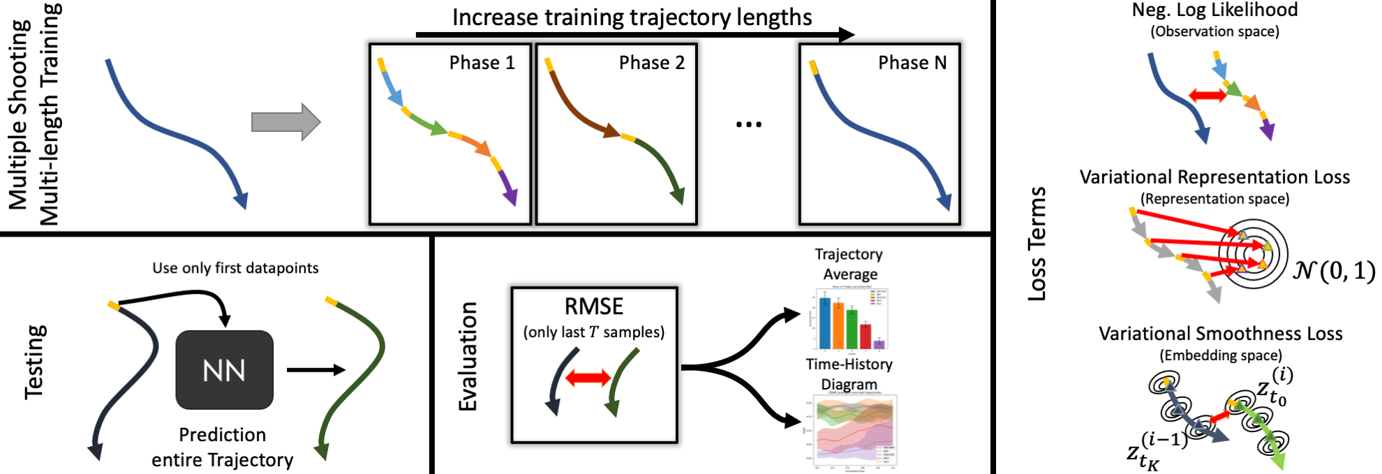
Figure 2: Training scheme with losses, and test/evaluation procedure. Top left: Multiple Shooting Multi-length Training. An input trajectory is split into subpatches. Subtrajectory length is increased in multiple phases to the length of the input trajectory. Bottom left: Testing: only the first few points are used to roll-out the latent trajectory and transformed to the observational space. Evaluation: Last $T$ samples of the predicted trajectory are used to compute the evaluation metrics, the average of the summed normalized mean squared error and a time history diagram showing the error evolution. Right: Loss consisting of three parts: negative log likelihood loss to penalize reconstruction errors, representation loss to define a gradient field between representations, smoothness loss to penalize jumps between latent subpatches.

Training.

We train all experiments in a multi-phase schedule wrt the multiple shooting loss in eq. 2. In the different phases, we split the input trajectory into overlapping patches and start learning by predicting one step ahead. We double the number of prediction steps per patch every 3000 epochs meaning that learning is done on longer patches with decreased number of patches per trajectory. In cases where the trajectory length is not divisible by the number of prediction steps, we drop the last patch and scale the loss accordingly. In the final phase, training is carried out on the entire trajectory. All network architectures are implemented in the open source framework PyTorch [38]. Further training details and hyperparameters can be found in Appendix A.

Testing. We test the trained models on entirely unseen trajectories. During testing, we only provide the first $k{=}10$ trajectory points to the learned model. Based on these samples, we compute a trajectory representation $\psi^{r}$ followed by rolling out the latent trajectory at the time points of interest. Finally, we compare predictions and ground truth observations by evaluation metrics.

Evaluation metrics. Our experiments focus on two key metrics. Firstly, we calculate the mean squared error (MSE) for extrapolated trajectories, where we evaluate the model’s performance over a total of $2T$ steps and measure the MSE over the last $T$ timesteps. This approach allows us to assess whether extrapolation over future time periods can better predict the model’s ability to extrapolate further in time, compared to reconstruction MSE. The value of $T$ is set to 60 for all our experiments, and we normalize the MSE value by dividing it with the average intensity of the ground truth observation, as recommended in [48, 4]. Additionally, we provide time history diagrams that plot the root mean square error (RMSE) against the normalized time, which maps the time interval $[T,2T]$ to the interval $[0,1]$. All evaluation metrics presented are averaged across all test trajectories and five runs, with mean and $75\%$ inter-quartile range (IQR) reported on all metrics. Last, we also provide subsampled predictions and the pixelwise $L_{2}$ error of one trajectory for visual inspection but we emphasize that one trajectory might not be representative for the overall performance (the trajectory shown is chosen at random). Please see Figure 2 for visual intuition on the training and testing procedure and how evaluation metrics are applied.

6 Results

We report on a series of increasingly challenging experiments to test LaDID. First, we examined whether our model generalizes well on synthetic data for which the training and test data come from the same dynamical system. This body of experiments test whether the model can learn to map from a finite, empirical dataset to an effective latent dynamical model. Second, we examined few-shot generalization to data obtained from systems subject to nontrivial intervention (and in that sense strongly out-of-distribution). In particular, we train our model on a set of trajectories under interventions, i.e. interventions upon the mass or length of the pendulum, changes to the Reynolds number, or variations to the camera view on the observed system, and apply the learned inductive bias to new and unseen interventional regimes in a few-shot learning setting. This tests the hypothesis that the inductive bias of our learned latent dynamical models can be a useful proxy for dynamical systems exposed to a number of interventions.

6.1 Benchmark comparisons to state-of-the-art models for ODE and PDE problems

We begin by investigating whether our approach can learn latent dynamical models in the conventional case in which the training and test data come from the same system. We evaluate the performance of ODE-RNN, ODE2VAE, NODEP, MSVI and LaDID on data described in Sec. 4 and Sec. B of the Appendix with increasing order of difficulty, starting with the non-linear mechanical swing systems with underlying ODEs, before moving to non-linear cases based on PDEs (reaction-diffusion system, 2D wave equation, von Kármán vortex street at the transition from laminar to turbulent flows, and Naiver-Stokes equations). We only present results for a subset of performed experiments here but refer the interested reader to Appendix C for a detailed presentation of all results.

Applications to ODE-based systems. For visual inspection and intuition, Figure 3(c) provides predicted observations $\hat{x}_{t}^{r}$ of a few time points of one test trajectory of the single pendulum dataset for all tested algorithms, followed by the ground truth trajectory and the pixelwise $L_{2}$-error. In addition, Figure 3(a) presents the normalized MSE over entire trajectories averaged across the entire test dataset and the evolution of the RMSE over time for the second half of the predicted observations averaged over all test trajectories (see Sec. 5) is provided in Fig. 3(b). First, we see that across all ODE-based datasets LaDID achieves consistently the lowest normalized MSE. Second, the time history diagram (see Fig. 3 in the Appendix) shows that LaDID predicts future time points with lower mean RMSE and lower standard deviation for long-horizon predictions relative to the other algorithms tested.

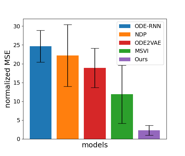
(a) Normalized MSE

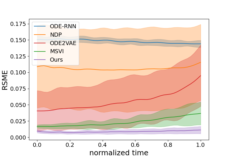
(b) RMSE distribution over time

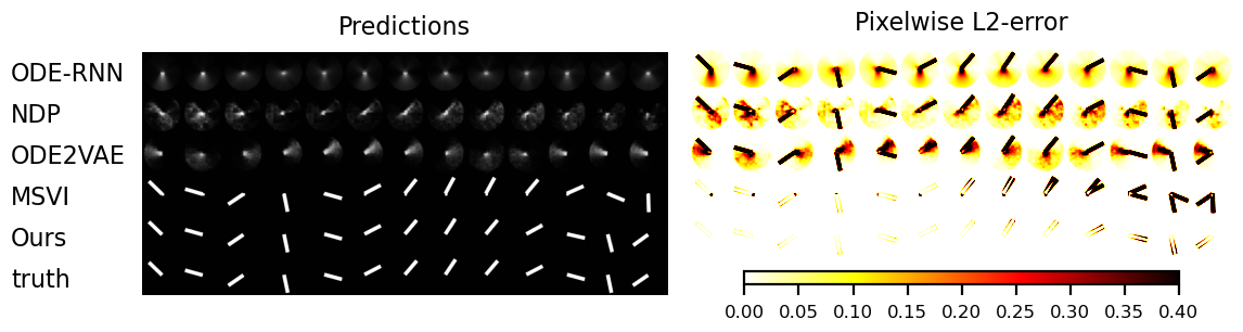
(c) Example trajectory

Figure 3: Test errors and exemplary test trajectories of different models for the single pendulum test case.

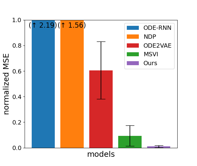
(a) Normalized MSE

(b) RMSE distribution over time

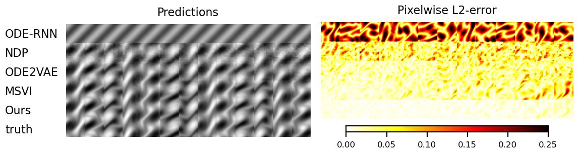
(c) Example trajectory

Figure 4: Test errors and exemplary test trajectories of different models for the Navier-Stokes equations test case.

This can also seen by visual inspection in Figure 3(c) as for other approaches the predicted states at later time points deviate from the ground truth trajectory substantially while LaDID’s predictions follow the ground truth. Considering only the baselines, one can observe that MSVI (a recent and sophisticated approach), achieves the best results and predicts accurately within a short-term horizon but fails on long-horizon predictions. The results for the challenging double pendulum test case can be found in the Appendix.

Applications to PDE-based processes. We additionally evaluated all baselines and our proposed method on PDE-based processes. Due to space restrictions, we focus our analysis on the flow evolution characterized by the Navier-Stokes equation in the two dimensional case, which is of importance in many engineering tasks, e.g. the analysis of internal air flow in a combustion engine [5, 29], drag reduction concepts in the transportation and energy sector [18, 36, 35], and many more. Results in Figure 4 show that LaDID clearly outperforms all considered comparators in terms of normalized MSE and averaged RMSE. This is echoed in the other experiments whose results are presented in detail in Sec. C in the Appendix.

Overall, the results shown (see also Sec. C for the complete collection of experimental results) support the notion that LaDID can achieve state-of-the-art performance for ODE and PDE based systems.

Performance on regular and irregular time grids. Here, we study the performance of LaDID on regular and irregular time grids and compare it to other neural-dynamical models (which are able to deal with irregular time series data). As shown in Fig. 5, the proposed LaDID performs very similarly on both types of the time grids relative to both ODE-based benchmark examples and challenging PDE-based real-world systems, outperforming existing methods in these test cases with irregularly sampled data.

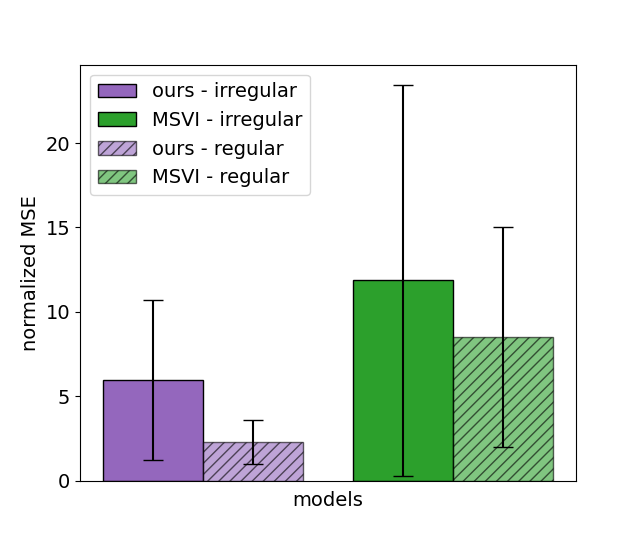
(a) Single pendulum: Normalized MSE

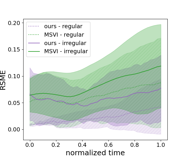
(b) Sigle pendulum: RMSE distribution over time

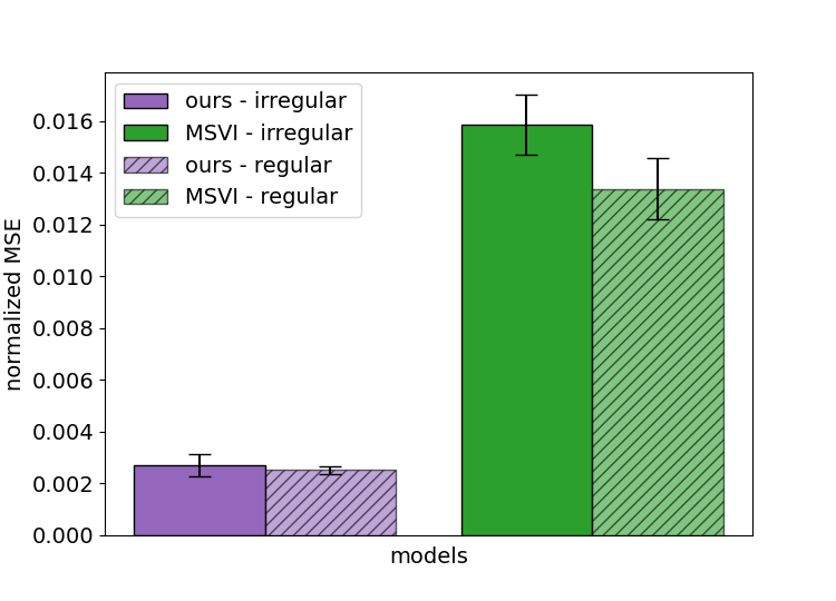
(c) Lambda-omega reaction-diffusion system: Normalized MSE

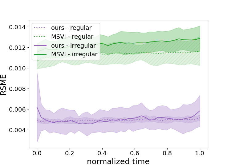
(d) Lambda-omega reaction-diffusion systemRMSE distribution over time

Figure 5: Test errors of different models for regular and irregular time grids: (a) Normalized MSE for single pendulum dataset, (b) RMSE over time for single pendulum dataset, (c) Normalized MSE for lambda-omega reaction-diffusion system, (d) RMSE over time for lambda-omega reaction-diffusion system.

Table 1: Errors for ablated LaDID models trained on the single pendulum test case.

loss heuristics			attention mechanism			representation encoding
ablation	mean	IQR	ablation	mean	IQR	ablation	mean	IQR
reconstruction	2.66	1.04	no attention	7.79	6.84	w./o. encoding	2.83	2.02
reconstruction & representation	2.17	0.99	spatial attention	2.81	1.47	w. encoding	2.02	0.88
reconstruction & smoothness	2.04	0.92	temporal attention	2.41	0.92
full loss	2.02	0.88	spatio-temporal attention	2.02	0.88

Effects of relevant network modules. As discussed above, our model leverages three key features: a reconstruction embedding, a spatio-temporal attention module and a specifically designed loss heuristic to learn temporal dynamics from empirical data. Here, we show that each of these network modules is indeed relevant for the performance of LaDID (see Tab. 1). First, we compare LaDID with counterparts trained on ablated loss heuristics, e.g. a pure reconstruction loss and loss combinations either using the described representation or smoothness loss. Overall, the proposed loss heuristic appears to stabilize training and yields the lowest MSE and IQR values. Second, we compare LaDID to counterparts trained on ablated attention modules. Tab. 1 highlights that the applied spatio-temporal attention helps to extract key dynamical patterns. Finally, Tab. 1 further shows the usefulness of the proposed representation encoding. This representation encoding can be thought of a learning-enhanced initial value stabilizing the temporal evolution of latent trajectory dynamics.

6.2 Generalizing to novel systems via few-shot learning

Here, we assess LaDID’s ability to generalize to a novel system obtained by nontrivial intervention on the system coefficients themselves (e.g., mass, length, Reynolds number). Such changes can induce large changes to data distributions (and can also be viewed through a causal lens). In this context, we aim to transfer the inductive bias learned from a set of training systems to a new set of systems with limited data availability in a few-shot learning setup. In particular, we train a dynamical model on a set of interventions and fine-tune it to new intervention regimes with only a few samples, finally evaluating performance on an entirely unseen dataset. We compare the performance of our prior-based few-shot learning model with a model trained solely on the fine-tuning dataset (“scratch” trained model). In our first experiment, we use the single pendulum dataset and test the transferability hypothesis on fine-tuning datasets of varying sizes. The results show that the prior-based model outperforms the scratch-trained model at all fine-tuning dataset sizes, and achieves comparable performance to the model trained on the full dataset with a fine-tuning dataset size of $32\%$. At a fine-tuning dataset size of $8\%$, LaDID produces partially erroneous but still usable predictions, only slightly worse than the predictions of a recent NODE based model, MSVI, trained on the full dataset.

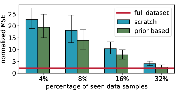
(a) single pendulum

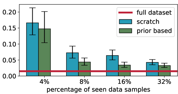
(b) vortex street

Figure 6: Test errors for a set of experiments involving transfer to nontrivial interventions (see text for details).

In the second experiment, we investigate the effect of interventions on the observation process by testing the transferability of our model to new observation settings on the von Kármán vortex street dataset. We re-simulate different cylinder locations (shifted the cylinder to the left, right, up, and down) and evaluate performance with different fine-tuning dataset sizes. We find that the prior-based model outperforms the scratch-trained model and produces accurate and usable predictions under new conditions with a fine-tuning dataset size of as small as $8\%$. These findings support the notion that LaDID is capable of extracting generalizable dynamical models from training data.

7 Discussion

In this paper, we presented a novel approach called LaDID aimed at end-to-end learning of latent dynamical models from empirical data. LaDID uses a novel transformer-based architecture that leverages certain scientifically-motivated invariances to allow separation of a universal dynamics module and encoded realization-specific information. We demonstated state-of-the-art performance on several new and challenging test cases and well-known benchmarks. Additionally, we showed that LaDID can generalize to systems under nontrivial intervention (when trained on the un-intervened system) using few-shot learning, and in that sense provides a potentially useful way to model systems under novel interventions.

However, despite good performance relative to NODE-based methods, for complex models prediction over very long time horizons remains challenging and further modifications and possibly additional inductive bias will be needed for improved performance. At present, data sampled on an irregular spatial grid cannot be considered. Future work using graph-based approaches will address this point.

Our work was motivated by the broad range of examples in contemporary science and engineering in which data are available from different experiments/pipelines that are plausibly underpinned by a unified model but where the model itself cannot be directly specified from first principles or is too complex to work with. A key motivation for our work is problems in the biomedical and health domains, where we expect the invariances underpinning LaDID to hold, but where explicit dynamical models are often not available at the outset. In ongoing work we are exploring the use of LaDID and related schemes in these challenging settings, e.g. for the modelling of complex longitudinal observations. In such settings, an implicit yet universal model is useful as a way to capture system behaviour and to generalize, in a data efficient manner, to new realizations/instances where only limited data may be available.

Appendix A Training details and hyperparameters

Our implementation uses the PyTorch framework [38]. All modules are initialized from scratch using random weights. During training, an AdamW-Optimizer [31] is applied starting at an initial learning rate $\varepsilon_{0}=0.0003$. An exponential learning rate scheduler is applied showing the best results in the current study. Every network is trained for 30 000 epochs. At initialization, we start training at a subpatch length of 1 which is doubled every 3000 epochs. After the CNN encoder, 8 attention layers are stacked each using 4 attention heads. A relative Sin/Cos embedding is used as position encoding followed by a linear layer. The input resolution of the observational image data is $128\times 128$ px. All computations are run on a single GPU node equipped with one NVidia A100 (40 GB) and a global batch size of 16 is used. A full training run on the single pendulum, the double pendulum, the wave equation and the Navier-Stokes equation dataset requires approx. 14 h. A full training run on the reaction-diffusion system and the von Kármán vortex street requires approx. 8 h.

Table 2: Training hyperparameters

Hyperparameter	Value
LR schedule	Exp. decay
Initial LR	3e-4
Weight Decay	0.01
Global batch size	16
Parallel GPUs	1
Input resolution	$128\times 128$ px
Number of input timesteps	10
Initial subpatch length	1
Number of epochs per subpatch length	3000
Latent dimension	32
attention mechanism	spatio-temporal
Number of attention blocks	8
Number of attention heads	4
Position Encoding	relative Sin/Cos encoding

Appendix B Dataset details

Here, we provide details about the datasets used in this work, their underlying mathematical formulations and their implementation details. Partially, some of the datasets we selected are used in literature to demonstrate the effectiveness of neural based temporal modeling approaches, e.g., a swinging pendulum or a reaction-diffusion system. However, we also consider more unknown test cases which represent complex real-world applications such as the chaotic double-pendulum or fluid flow applications driven by a complex set of PDEs, i.e., the Navier-Stokes equations.

B.1 Swinging pendulum

For the first dataset we consider synthetic videos of a nonlinear pendulum simulated in two spatial dimensions. Typically, a nonlinear swinging pendulum is governed by the following second order differential equation:

$$\frac{d^{2}z}{dt^{2}}=-\sin z$$ (3)

with $z$ denoting the angle of the pendulum. Overall, we simulated 500 trajectories with different initial conditions. For each trajectory, the initial angle $z$ and its angular velocity $\frac{dz}{dt}$ is sampled uniformly from $z\sim\mathcal{U}(0,2\pi)$ and $\frac{dz}{dt}\sim\mathcal{U}(-\pi/2,\pi/2)$. All trajectories are simulated for $t=3$ seconds. The training, validation and test dataset is split into 400, 50 and 50 trajectories, respectively. The swinging pendulum is rendered in black/white image space over 128 pixels for each spatial dimension. Hence, each observation is a high-dimensional image representation (16384 dimensions - flattened $128\times 128\,\textrm{px}^{2}$ image) of an instantaneous state of the second-order ODE.

B.2 Swinging double pendulum

To increase the complexity of the second dataset, we selected the kinematics of a nonlinear double pendulum motion. The pendulums are treated as two point masses with the upper pendulum being denoted by the subscript ”1” and the lower one by subscript ”2”. The kinematics of this nearly chaotic system is governed by the following set of ordinary differential equations:

$$\frac{d^{2}z_{1}}{dt^{2}}=\frac{-g(2m_{1}+m_{2})\sin z_{1}-m_{2}g\sin(z_{1}-2z_{2})-2\sin(z_{1}-z_{2})m_{2}(\frac{dz_{1}}{dt}^{2}L_{2}+\frac{dz_{1}}{dt}^{2}L_{1}\cos(z_{1}-z_{2}))}{L_{1}(2m_{1}+m_{2}-m_{2}\cos(2z_{1}-2z_{2}))}$$ (4)

$$\frac{d^{2}z_{2}}{dt^{2}}=\frac{2\sin(z_{1}-z_{2})(\frac{dz_{1}}{dt}^{2}L_{1}(m_{1}+m_{2})+g(m_{1}+m_{2})\cos z_{1}+\frac{dz_{2}}{dt}^{2}L_{2}m_{2}\cos(z_{1}-z_{2}))}{L_{2}(2m_{1}+m_{2}-m_{2}\cos(2z_{1}-2z_{2}))}$$ (5)

with $m_{i}$ denoting the mass and the length of each pendulum respectively, and $g$ is the gravitational constant. Again, we simulated 500 trajectories split in sets of 400, 50 and 50 samples for training, validation and testing. The initial condition for $(z_{1},z_{2})$ and $(\frac{dz_{1}}{dt},\frac{dz_{2}}{dt})$ are uniformly sampled in the range $\mathcal{U}(0,2\pi)$ and $\mathcal{U}(-\pi/2,\pi/2)$. The double pendulum is rendered in a RGB color space over 128 pixels for each spatial dimension with the first pendulum colored in red and the second one in green. Hence, each observation is a high-dimensional image representation ($16384\times 3$ dimensions - flatted $128\times 128\,\textrm{px}^{2}$ RGB image) of an instantaneous double pendulum state.

B.3 Reaction-diffusion equation

Many real-world applications of interest originate from dynamics governed by partial differential equations with more complex interactions between spatial and temporal dynamics. One such set of PDEs we selected as test case is based on a lambda-omega reaction-diffusion system which is described by the following equations:

$$\frac{du}{dt}=(1-(u^{2}+v^{2}))u+\beta(u^{2}+v^{2})v+d_{1}(\frac{d^{2}u}{dx^{2}}+\frac{d^{2}u}{dy^{2}})$$ (6)

$$\frac{dv}{dt}=-\beta(u^{2}+v^{2})u+(1-(u^{2}+v^{2}))v+d_{2}(\frac{d^{2}v}{dx^{2}}+\frac{d^{2}v}{dy^{2}})$$ (7)

with $(d_{1},d_{2})=0.1$ denoting diffusion constants and $\beta=1$. This set of equations generates a spiral wave formation which can be approximated by two oscillating spiral modes. The system is simulated from a single initial condition from $t=0$ to $t=10$ in $\Delta t=0.05$ time intervals for a total number of 10 000 samples. The initial conditions is defined as

$$u(x,y,0)=\mathrm{tanh}\left(\sqrt{x^{2}+y^{2}}\cos\left((x+iy)-\sqrt{x^{2}-y^{2}}\right)\right)$$ (8)

$$v(x,y,0)=\mathrm{tanh}\left(\sqrt{x^{2}+y^{2}}\sin\left((x+iy)-\sqrt{x^{2}-y^{2}}\right)\right).$$ (9)

The simulation is performed over a spatial domain of $(x\in[-10,10]$ and $y\in[-10,10]$ on grid with 128 points in each spatial dimension. We split this simulation into trajectories of 50 consecutive samples resulting in 200 in dependant realisations. We use 160 randomly sampled trajectories for training, 20 trajectories for validation and the remaining 20 trajectories for testing. Source code of the simulation can be found in [7].

B.4 Two-dimensional wave equation

A classical example of a hyperbolic PDE is the two-dimensional wave equation describing the temporal and spatial propagation of waves such as sound or water waves. Wave equations are important for a variety of fields including acoustics, electromagnetics and fluid dynamics. In two dimensions, the wave equation can be described as follows:

$$\frac{\partial^{2}u}{\partial t^{2}}=c^{2}\triangledown^{2}u,$$ (10)

with $\triangledown^{2}$ denoting the Laplacian operator in $\mathcal{R}^{2}$ and $c$ is a constant speed of the wave propagation. The initial displacement $u_{0}$ is a Gaussian function

$$u_{0}=a\exp\left(-\frac{(x-b)^{2}}{2r^{2}}\right),$$ (11)

where the amplitude of the peak displacement $a$, the location of the peak displacement $b$ and the standard deviation $r$ are uniformly sampled from $a\sim\mathcal{U}(2,4)$, $b\sim\mathcal{U}(-1,1)$, and $r\sim\mathcal{U}(0.25,0.30)$, respectively. Similar to [45], the inital velocity gradient $\frac{\partial u}{\partial t}$ is set to zero. The wave simulations are performed over a spatial domain of $(x\in[-1,1]$ and $y\in[-1,1]$ on a grid with 128 points in each spatial dimension. Overall, 500 independent trajectories (individual initial conditions) are computed which are split in 400 randomly sampled trajectories for training, 50 trajectories for validation and the remaining 50 trajectories for testing.

B.5 Navier-Stokes equations

To ultimately test the performance of our model on complex real-world data, we simulated fluid flows governed by a complex set of partial differential equations called Navier-Stokes equations. Overall, two flow cases of different nature are considered, e.g., the temporal evolution of generic initial vorticity fields and the flow around an obstacle characterized by the formations of dominant vortex patterns also known as the von Kármán vortex street.
Due to the characteristics of the selected flow fields, we consider the incompressible two-dimensional Navier-Stokes equations given by

$$\frac{\partial u}{\partial t}+(u\cdot\triangledown)u-\nu\triangledown^{2}u=-\frac{1}{\rho}\triangledown p.$$ (12)

Here, $u$ denotes the velocity in two dimensions, $t$ and $p$ are the time and pressure, and $\nu$ is the kinematic viscosity. For the generic test case, we solve this set of PDEs in its vorticity form and chose initial conditions as described in [30]. Simulations are performed over a spatial domain of $(x\in[-1,1]$ and $y\in[-1,1]$ on a grid with 128 points in each spatial dimension. Overall, 500 independent trajectories (individual initial vorticity fields) are computed which are split in 400 randomly sampled trajectories for training, 50 trajectories for validation and the remaining 50 trajectories for testing.

B.6 Flow around a blunt body

The second fluid flow case mimics an engineering inspired applications and captures the flow around a blunt cylinder body, also known as von Kármán vortex street. von Kármán vortices manifest in a repeating pattern of swirling vortices caused by the unsteady flow separation around blunt bodies and occur when the inertial forces in a flow are significantly greater than the viscous forces. A large dynamic viscosity of a fluid suppresses vortices, whereas a higher density, velocity, and larger size of the flowed object provide for more dynamics and a less ordered flow pattern. If the factors that increase the inertial forces are put in relation to the viscosity, a dimensionless measure - the Reynolds number - is obtained that can be used to characterize a flow regime. If the Reynolds number is larger than $Re>80$, the two vortices in the wake of the body become unstable until they finally detach periodically. The detached vortices remain stable for a while until they slowly dissociate again in the flow due to friction, and finally disappear. The incompressible vortex street is simulated using an open-source Lattice-Boltzmann solver due to computational efficiency. The governing equation is the Boltzmann equation with the simplified right-hand side (RHS) Bhatnagar-Gross-Krook (BGK) collision term [3]:

$$\frac{\partial f}{\partial t}+\zeta_{k}\frac{\partial f}{\partial x_{k}}=-\frac{1}{\tau}(f-f^{eq})$$ (13)

These particle probability density functions (PPDFs) $f=f(\vec{x},\vec{\zeta},t)$ describe the probability to find a fluid particle around a location $\vec{x}$ with a particle velocity $\vec{\zeta}$ at time $t$ [2]. The left-hand side (LHS) describes the evolution of fluid particles in space and time, while the RHS describes the collision of particles. The collision process is governed by the relaxation parameter $1/\tau$ with the relaxation time $\tau$ to reach the Maxwellian equilibrium state $f^{eq}$. The discretized form of equation 13 yield the lattice-BGK equation

$$f_{k}(\vec{x}+\zeta_{k}\Delta t,t+\Delta t)=f_{k}(\vec{x},t)-\frac{1}{\tau}(f_{k}(\vec{x},t)-f_{k}^{eq}(\vec{x},t)).$$ (14)

The standard $D_{2}Q_{9}$ discretization scheme with nine PPDFs [39] is applied. The equilibrium PPDF is given by

$$f_{k}^{eq}=w_{k}\rho\left(1+\frac{\zeta_{k}\vec{u}}{c_{s}^{2}}+\frac{(\zeta_{k}\vec{u})^{2}}{2c_{s}^{4}}-\frac{\vec{u}^{2}}{2c_{s}^{2}}\right)$$ (15)

where the quantities $w_{k}$ are weighting factors for the $D_{2}Q_{9}$ scheme given by $4/9$ for $k\in{0}$, $1/9$ for $k\in{1,\dots,4}$, and $1/36$ for $k\in{5,\dots 9}$, and $\vec{u}$ is the fluid velocity. $c_{s}$ denotes the speed of sound. The makroscopic variables can be obtained from the moments of the PPDFs. Within the continuum limit, i.e., for small Knudsen numbers, the Navier-Stokes equations can directly be derived from the Boltzmann equation and the BGK model [21]. We simulated three different Reynolds numbers $Re=100,250,500$ for 425 000 iterations with a mesh size of 128 point in vertical and 256 points in horizontal direction. We skipped the first 25 000 iterations to ensure a developed flow field and extracted velocity snapshot every 100 iterations. The simulation is performed over a spatial domain of $(x\in[-20,20]$ and $y\in[-10,10]$. We split this simulation into trajectories of 50 consecutive samples resulting in 200 in dependant realisations. We use 160 randomly sampled trajectories for training, 20 trajectories for validation and the remaining 20 trajectories for testing.

Appendix C Additional results

C.1 Swinging double pendulum

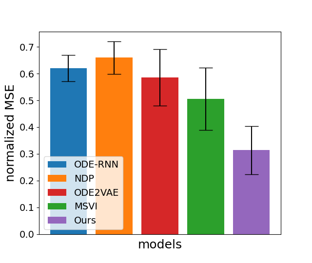
(a) Normalized MSE

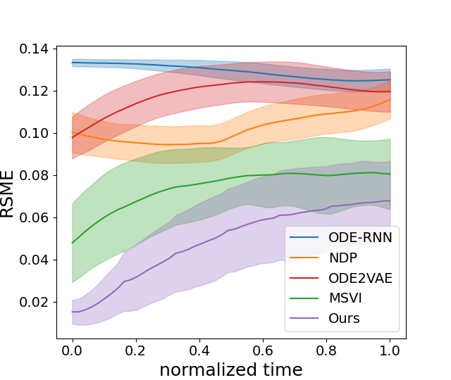
(b) RMSE distribution over time

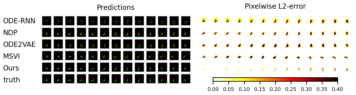
(c) Example trajectory

Figure C.1: Test errors and exemplary test trajectories of different models for the double pendulum test case.

C.2 Lambda-omega reaction-diffusion system

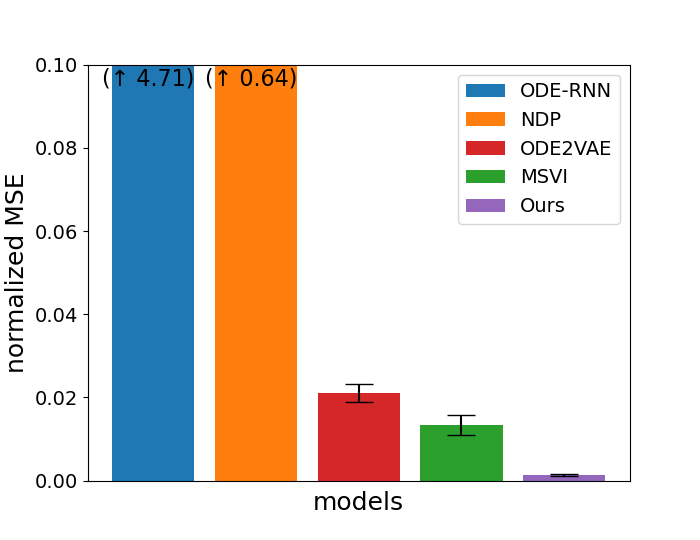
(a) Normalized MSE

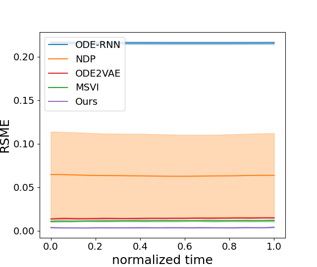
(b) RMSE distribution over time

(c) Example trajectory

Figure C.2: Test errors and exemplary test trajectories of different models for the lambda-omega reaction-diffusion system.

C.3 Two-dimensional wave equation

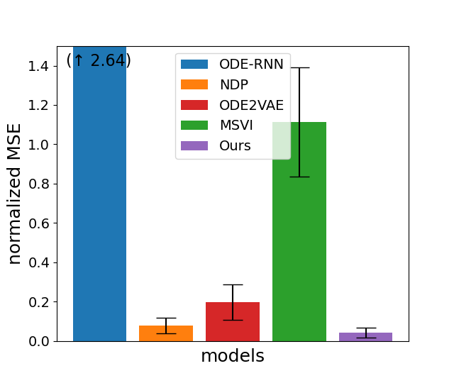
(a) Normalized MSE

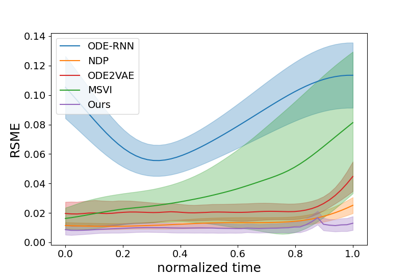
(b) RMSE distribution over time

(c) Example trajectory

Figure C.3: Test errors and exemplary test trajectories of different models for the wave equation test case.

C.4 Latticed Boltzmann equations

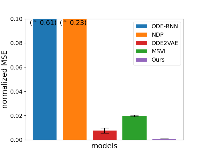
(a) Normalized MSE

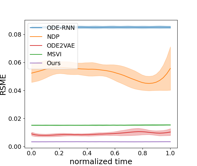
(b) RMSE distribution over time

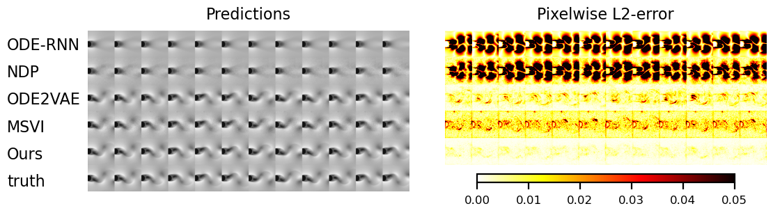
(c) Example trajectory

Figure C.4: Test errors and exemplary test trajectories of different models for the von Kármán vortex street test case.

References

- [1] Shaojie Bai, J Zico Kolter, and Vladlen Koltun. Deep equilibrium models. Advances in Neural Information Processing Systems, 32, 2019.
- [2] Roberto Benzi, Sauro Succi, and Massimo Vergassola. The lattice boltzmann equation: theory and applications. Physics Reports, 222(3):145–197, 1992.
- [3] Prabhu Lal Bhatnagar, Eugene P Gross, and Max Krook. A model for collision processes in gases. i. small amplitude processes in charged and neutral one-component systems. Physical review, 94(3):511, 1954.
- [4] Aleksandar Botev, Andrew Jaegle, Peter Wirnsberger, Daniel Hennes, and Irina Higgins. Which priors matter? benchmarking models for learning latent dynamics. Advances in Neural Information Processing Systems, 34, 2021.
- [5] Marco Braun, Wolfgang Schröder, and Michael Klaas. High-speed tomographic PIV measurements in a DISI engine. Experiments in Fluids, 60(9):146, 2019.
- [6] Steven L. Brunton, Joshua L. Proctor, and J. Nathan Kutz. Discovering governing equations from data by sparse identification of nonlinear dynamical systems. Proceedings of the National Academy of Sciences, 113(15):3932–3937, 2016.
- [7] Kathleen Champion, Bethany Lusch, J Nathan Kutz, and Steven L Brunton. Data-driven discovery of coordinates and governing equations. Proceedings of the National Academy of Sciences, 116(45):22445–22451, 2019.
- [8] Ricky T. Q. Chen, Brandon Amos, and Maximilian Nickel. Learning neural event functions for ordinary differential equations. International Conference on Learning Representations, 2021.
- [9] Ricky TQ Chen, Yulia Rubanova, Jesse Bettencourt, and David K Duvenaud. Neural ordinary differential equations. Advances in Neural Information Processing Systems, 31, 2018.
- [10] Matthew Choi, Daniel Flam-Shepherd, Thi Ha Kyaw, and Alán Aspuru-Guzik. Learning quantum dynamics with latent neural ordinary differential equations. Physical Review A, 105(4):042403, 2022.
- [11] Miles Cranmer, Sam Greydanus, Stephan Hoyer, Peter Battaglia, David Spergel, and Shirley Ho. Lagrangian neural networks. arXiv preprint arXiv:2003.04630, 2020.
- [12] Thai Duong and Nikolay Atanasov. Hamiltonian-based Neural ODE Networks on the SE(3) Manifold For Dynamics Learning and Control. In Proceedings of Robotics: Science and Systems, 2021.
- [13] Emilien Dupont, Arnaud Doucet, and Yee Whye Teh. Augmented neural odes. Advances in Neural Information Processing Systems, 32, 2019.
- [14] Weinan E. A proposal on machine learning via dynamical systems. Communications in Mathematics and Statistics, 5(1):1–11, 2017.
- [15] Charles Fefferman, Sanjoy Mitter, and Hariharan Narayanan. Testing the manifold hypothesis. Journal of the American Mathematical Society, 29(4):983–1049, 2016.
- [16] Chris Finlay, Jörn-Henrik Jacobsen, Levon Nurbekyan, and Adam Oberman. How to train your neural ode: the world of jacobian and kinetic regularization. In International conference on machine learning, pages 3154–3164. PMLR, 2020.
- [17] Marc Finzi, Ke Alexander Wang, and Andrew G Wilson. Simplifying hamiltonian and lagrangian neural networks via explicit constraints. Advances in Neural Information Processing Systems, 33, 2020.
- [18] Erwin R Gowree, Chetan Jagadeesh, Edward Talboys, Christian Lagemann, and Christoph Brücker. Vortices enable the complex aerobatics of peregrine falcons. Communications biology, 1(1):27, 2018.
- [19] Samuel Greydanus, Misko Dzamba, and Jason Yosinski. Hamiltonian neural networks. Advances in Neural Information Processing Systems, 32, 2019.
- [20] Eldad Haber and Lars Ruthotto. Stable architectures for deep neural networks. Inverse Problems, 34(1):014004, 2017.
- [21] Dieter Hänel. Molekulare Gasdynamik: Einführung in die kinetische Theorie der Gase und Lattice-Boltzmann-Methoden. Springer-Verlag, 2006.
- [22] Markus Heinonen, Cagatay Yildiz, Henrik Mannerström, Jukka Intosalmi, and Harri Lähdesmäki. Learning unknown ODE models with Gaussian processes. In International Conference on Machine Learning, pages 1959–1968. PMLR, 2018.
- [23] Valerii Iakovlev, Cagatay Yildiz, Markus Heinonen, and Harri Lähdesmäki. Latent neural ODEs with sparse bayesian multiple shooting. In The Eleventh International Conference on Learning Representations, 2023.
- [24] Junteng Jia and Austin R Benson. Neural jump stochastic differential equations. Advances in Neural Information Processing Systems, 32, 2019.
- [25] Kadierdan Kaheman, J. Nathan Kutz, and Steven L. Brunton. SINDy-PI: a robust algorithm for parallel implicit sparse identification of nonlinear dynamics. Proceedings of the Royal Society A: Mathematical, Physical and Engineering Sciences, 476(2242), 2020.
- [26] Patrick Kidger, James Morrill, James Foster, and Terry Lyons. Neural controlled differential equations for irregular time series. Advances in Neural Information Processing Systems, 33, 2020.
- [27] Timothy D Kim, Thomas Z Luo, Jonathan W Pillow, and Carlos D Brody. Inferring latent dynamics underlying neural population activity via neural differential equations. In International Conference on Machine Learning, pages 5551–5561. PMLR, 2021.
- [28] Diederik P Kingma and Max Welling. Auto-encoding variational bayes. arXiv preprint arXiv:1312.6114, 2013.
- [29] Christian Lagemann, Kai Lagemann, Sach Mukherjee, and Wolfgang Schroeder. Generalization of deep recurrent optical flow estimation for particle-image velocimetry data. Measurement Science and Technology, 2022.
- [30] Zongyi Li, Nikola Kovachki, Kamyar Azizzadenesheli, Burigede Liu, Kaushik Bhattacharya, Andrew Stuart, and Anima Anandkumar. Fourier neural operator for parametric partial differential equations. In The Eighth International Conference on Learning Representations, 2020.
- [31] Ilya Loshchilov and Frank Hutter. Decoupled weight decay regularization. arXiv preprint arXiv:1711.05101, 2017.
- [32] Yiping Lu, Aoxiao Zhong, Quanzheng Li, and Bin Dong. Beyond finite layer neural networks: Bridging deep architectures and numerical differential equations. In International Conference on Machine Learning, pages 3276–3285. PMLR, 2018.
- [33] Michael Lutter, Christian Ritter, and Jan Peters. Deep lagrangian networks: Using physics as model prior for deep learning. In International Conference on Learning Representations, 2019.
- [34] Stefano Massaroli, Michael Poli, Sho Sonoda, Taiji Suzuki, Jinkyoo Park, Atsushi Yamashita, and Hajime Asama. Differentiable multiple shooting layers. Advances in Neural Information Processing Systems, 34:16532–16544, 2021.
- [35] Esther Mäteling, Marian Albers, and Wolfgang Schröder. How spanwise travelling transversal surface waves change the near-wall flow. Journal of Fluid Mechanics, 957:A30, 2023.
- [36] Esther Mäteling and Wolfgang Schröder. Analysis of spatiotemporal inner-outer large-scale interactions in turbulent channel flow by multivariate empirical mode decomposition. Physical Review Fluids, 7(3):034603, 2022.
- [37] James Morrill, Cristopher Salvi, Patrick Kidger, and James Foster. Neural rough differential equations for long time series. In International Conference on Machine Learning, pages 7829–7838. PMLR, 2021.
- [38] Adam Paszke, Sam Gross, Francisco Massa, Adam Lerer, James Bradbury, Gregory Chanan, Trevor Killeen, Zeming Lin, Natalia Gimelshein, Luca Antiga, Alban Desmaison, Andreas Köpf, Edward Yang, Zach DeVito, Martin Raison, Alykhan Tejani, Sasank Chilamkurthy, Benoit Steiner, Lu Fang, Junjie Bai, and Soumith Chintala. Pytorch: An imperative style, high-performance deep learning library, 2019.
- [39] Yue-Hong Qian, Dominique d’Humières, and Pierre Lallemand. Lattice BGK models for Navier-Stokes equation. Europhysics letters, 17(6):479, 1992.
- [40] Danilo Jimenez Rezende, Shakir Mohamed, and Daan Wierstra. Stochastic backpropagation and approximate inference in deep generative models. In International conference on machine learning, pages 1278–1286. PMLR, 2014.
- [41] Jack Richter-Powell, Yaron Lipman, and Ricky T. Q. Chen. Neural Conservation Laws: A Divergence-Free Perspective. In Advances in Neural Information Processing Systems, volume 35, 2022.
- [42] Yulia Rubanova, Ricky T. Q. Chen, and David K Duvenaud. Latent ordinary differential equations for irregularly-sampled time series. In Advances in Neural Information Processing Systems, volume 32, 2019.
- [43] Lars Ruthotto and Eldad Haber. Deep neural networks motivated by partial differential equations. Journal of Mathematical Imaging and Vision, 62:352–364, 2020.
- [44] Cagatay Yildiz, Markus Heinonen, and Harri Lahdesmaki. ODE2VAE: Deep generative second order ODEs with Bayesian neural networks. In Advances in Neural Information Processing Systems, volume 32, 2019.
- [45] Yuan Yin, Matthieu Kirchmeyer, Jean-Yves Franceschi, Alain Rakotomamonjy, and Patrick Gallinari. Continuous PDE Dynamics Forecasting with Implicit Neural Representations. In International Conference on Learning Representations, 2023.
- [46] Weiming Zhi, Tin Lai, Lionel Ott, Edwin V Bonilla, and Fabio Ramos. Learning efficient and robust ordinary differential equations via invertible neural networks. In International Conference on Machine Learning, pages 27060–27074. PMLR, 2022.
- [47] Yaofeng Desmond Zhong, Biswadip Dey, and Amit Chakraborty. Symplectic ODE-Net: Learning Hamiltonian Dynamics with Control. In International Conference on Learning Representations, 2020.
- [48] Yaofeng Desmond Zhong, Biswadip Dey, and Amit Chakraborty. Benchmarking energy-conserving neural networks for learning dynamics from data. In Proceedings of the 3rd Conference on Learning for Dynamics and Control, pages 1218–1229. PMLR, 2021.