End-to-End Augmentation Hyperparameter Tuning for Self-Supervised Anomaly Detection

Abstract

Self-supervised learning (SSL) has emerged as a promising paradigm that presents self-generated supervisory signals to real-world problems, bypassing the extensive manual labeling burden. SSL is especially attractive for unsupervised tasks such as anomaly detection, where labeled anomalies are often nonexistent and costly to obtain. While self-supervised anomaly detection (SSAD) has seen a recent surge of interest, the literature has failed to treat data augmentation as a hyperparameter. Meanwhile, recent works have reported that the choice of augmentation has significant impact on detection performance. In this paper, we introduce ST-SSAD (Self-Tuning Self-Supervised Anomaly Detection), the first systematic approach to SSAD in regards to rigorously tuning augmentation. To this end, our work presents two key contributions. The first is a new unsupervised validation loss that quantifies the alignment between the augmented training data and the (unlabeled) test data. In principle we adopt transduction, quantifying the extent to which augmentation mimics the true anomaly-generating mechanism, in contrast to augmenting data with arbitrary pseudo anomalies without regard to test data. Second, we present new differentiable augmentation functions, allowing data augmentation hyperparameter(s) to be tuned end-to-end via our proposed validation loss. Experiments on two testbeds with semantic class anomalies and subtle industrial defects show that systematically tuning augmentation offers significant performance gains over current practices.

1 Introduction

Anomaly detection (AD) finds many applications in security, finance, manufacturing, and surveillance, to name a few. Thanks to its popularity, the literature is abound with numerous detection techniques [1], while deep neural network-based AD models have attracted the most attention recently [2]. Especially for adversarial or dynamically-changing settings in which the anomalies are to be identified, it is important to design unsupervised techniques. While supervised detection can be employed for label-rich settings, unsupervised detection becomes critical to remain alert to emerging phenomena or the so-called “unknown unknowns”. Lack of ground-truth labels, however, makes it notoriously difficult to tune modern deep AD models with various hyperparameters [3].

Recently, self-supervised learning (SSL) has emerged as a promising paradigm that offers supervisory signals to real-world problems while avoiding the extensive cost of manual labeling, leading to great success in advancing NLP [4, 5] as well as computer vision tasks [6, 7]. SSL has become particularly attractive for unsupervised tasks such as AD, where labeled data is either nonexistent, costly to obtain, or nontrivial to simulate in the face of unknown anomalies. Thus, the literature has seen a recent surge of SSL-based AD (SSAD) techniques [8, 9, 10, 11, 12, 13].

The typical approach to SSAD involves incorporating self-generated pseudo anomalies into training, and then learning to separate those from the inliers. The pseudo anomalies are most often synthesized artificially by transforming inliers through a data augmentation function, such as masking, blurring, etc. (there is also work that “outlier-expose” the inliers to real samples from external data repos [9]).

In this paper, we address a fundamental challenge with SSAD, to which recent works seem to have turned a blind eye: recognizing and tuning augmentation as a hyperparameter. As shown recently by Yoo et al. [14], the choice of the augmentation function, as well as its associated argument(s) such as the masking amount, blurring level, etc., have tremendous impact on detection performance. This may come across as no surprise, or trivial to state, since the supervised learning community has long (and appropriately) integrated “data augmentation hyperparameters” into model selection [15, 16]. Meanwhile, there exists no such attempt in the SSAD literature (!). Although model selection without ground-truth labels is admittedly a much harder problem, turning a blind eye to the challenge may mislead by overstating the (unreasonable) effectiveness of SSL for unsupervised AD.

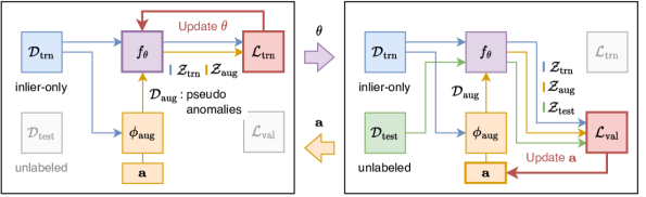
Figure 1: (left) Training and (right) validation (i.e. augmentation tuning) stages of ST-SSAD, which alternates between: (left) Given aug. function $\phi_{\mathrm{aug}}(\cdot;\mathbf{a})$, estimate the parameters $\theta$ of detector $f_{\theta}$ on inliers $\mathcal{D}_{\mathrm{trn}}$ and pseudo anomalies $\mathcal{D}_{\mathrm{aug}}$ via the training loss; (right) Given $f_{\theta}$ and (unlabeled) test data $\mathcal{D}_{\mathrm{test}}$, gradient-update the aug. hyperparameters $\mathbf{a}$ via our differentiable unsupervised validation loss that measures the agreement between $\mathcal{D}_{\mathrm{trn}}\cup\mathcal{D}_{\mathrm{aug}}$ and $\mathcal{D}_{\mathrm{test}}$ in the embedding space.

Our work introduces the first systematic approach to SSAD in regards to rigorously tuning augmentation. The key idea is to capitalize on transductive learning [17], where we leverage the unlabeled test data during self-supervised AD model tuning. Intuitively, SSL-based AD would work well as long as the augmentation-generated pseudo anomalies resemble the true anomalies (put differently, when the augmentation function well mimics the true anomaly-generating mechanism). To capture this insight, (1) we first design a novel, unsupervised validation loss for SSAD toward quantifying the alignment between the augmented training data and test data. Then, we propose to tune augmentation through our differentiable validation loss end-to-end (see Fig. 1). This necessitates the augmentation function to be differentiable as well. To this end, (2) we propose new differentiable formulations for popular augmentations such as CutOut (local) [18] and Rotation (global) [8] as proof of concept.

We argue that the use of (unlabeled) test data, containing the anomalies to be identified, during model tuning transductively is indeed exceedingly important for “success”. It is fundamentally different from existing SSAD approaches that “imagine” how the actual anomalies would look like or otherwise haphazardly choose augmentation that corresponds to some arbitrary notion of anomalies, which may not well align or agree with what is to be detected. Surely, one can incorporate expert/prior knowledge of anomalies in choosing augmentation, but in the absence thereof (recall unknown-unknowns), SSAD would likely fail as the recent study by Yoo et al. [14] documents.

Our extensive experiments on 41 anomaly detection tasks including both local and global anomalies show that ST-SSAD significantly outperforms both unsupervised and self-supervised baselines which rely on manual hyperparameter search without labels. Our qualitative analysis visually supports that ST-SSAD is capable of learning different augmentation hyperparameters for different anomaly types, even when they share the same normal data, by leveraging the anomalies in unlabeled test data. While in this paper we focus on image anomaly detection, our ST-SSAD framework is generally applicable to other input data modalities, provided such augmentation functions can be learned or designed.

2 Preliminaries

Notation    Let $\mathcal{D}_{\mathrm{trn}}$ denote a set of training normal (i.e. inlier) data, and $\mathcal{D}_{\mathrm{test}}$ be a set of test data containing both normal and anomalous samples. Let $\mathbf{x}\in\mathbb{R}^{d}$ denote a data sample in $\mathcal{D}_{\mathrm{trn}}\cup\mathcal{D}_{\mathrm{test}}$, where $d$ represents its dimension. Let $\phi_{\mathrm{aug}}(\mathbf{x},\mathbf{a})\in\mathbb{R}^{d}\times\mathcal{A}\mapsto\mathbb{R}^{d}$ depict a data augmentation function conditioned on hyperparameters $\mathbf{a}\in\mathcal{A}$, where $\mathcal{A}$ denotes possible values of the hyperparameters. For example, for $\phi_{\mathrm{aug}}$: rotation of an image, $\mathcal{A}=[0,360)$ is the domain of possible rotation angles. Let $f_{\theta}\in\mathbb{R}^{d}\mapsto\mathbb{R}^{h}$ be a detector parameterized by $\theta$, and $s\in\mathbb{R}^{h}\mapsto\mathbb{R}^{+}$ be an anomaly score function. Specifically, $f_{\theta}$ returns a low-dimensional embedding $\mathbf{z}\in\mathbb{R}^{h}$ for each sample $\mathbf{x}$, which is then fed into $s$ to compute the anomaly score of $\mathbf{x}$. We assume that $f_{\theta}$ is trained in a self-supervised fashion by creating a set $\mathcal{D}_{\mathrm{aug}}=\{\phi_{\mathrm{aug}}(\mathbf{x};\mathbf{a})\mid\mathbf{x}\in\mathcal{D}_{\mathrm{trn}}\}$ of pseudo anomalies using $\phi_{\mathrm{aug}}$.

Problem definition    Given $\mathcal{D}_{\mathrm{trn}}$ and $\mathcal{D}_{\mathrm{test}}$, how can we find $\mathbf{a}^{*}$ (along with the model parameters $\theta$) that maximizes the accuracy of the detector $f_{\theta}$ with score function $s$?

There is no trivial solution to the problem, since the labeled anomalies are not given at training time, but the problem is crucial for the success of SSAD in real-world tasks where the labels are hard to obtain or even nonexistent. To the best of our knowledge, this problem has not been studied in the literature, and our work is the first to propose a systematic solution to the problem.

3 Proposed Framework for End-to-End Augmentation Tuning

We propose ST-SSAD (Self-Tuning Self-Supervised Anomaly Detection), a framework for augmentation hyperparameter tuning in SSAD. Given test data $\mathcal{D}_{\mathrm{test}}$ which contains unlabeled anomalies, ST-SSAD automatically finds the best augmentation hyperparameter $\mathbf{a}^{*}$ that maximizes the semantic alignment between the augmentation function and the underlying anomaly-generating mechanism hidden in $\mathcal{D}_{\mathrm{test}}$. The search process is performed in an end-to-end fashion thanks to two core novel engines of ST-SSAD: (1) an unsupervised validation loss $\mathcal{L}_{\mathrm{val}}$ and (2) a differentiable augmentation function $\phi_{\mathrm{aug}}$, which we describe in detail in Sec. 3.1 and 3.2, respectively.

Fig. 1 shows an overall structure of ST-SSAD, which updates the parameters $\theta$ of the detector $f_{\theta}$ and the augmentation hyperparameters $\mathbf{a}$ through alternating stages for training and validation. Let $\mathcal{Z}_{\mathrm{trn}}=\{f_{\theta}(\mathbf{x})\mid\mathbf{x}\in\mathcal{D}_{\mathrm{trn}}\}$ be the embeddings of $\mathcal{D}_{\mathrm{trn}}$, $\mathcal{Z}_{\mathrm{aug}}=\{f_{\theta}(\phi_{\mathrm{aug}}(\mathbf{x};\mathbf{a}))\mid\mathbf{x}\in\mathcal{D}_{\mathrm{trn}}\}$ be the embeddings of augmented data, and $\mathcal{Z}_{\mathrm{test}}=\{f_{\theta}(\mathbf{x})\mid\mathbf{x}\in\mathcal{D}_{\mathrm{test}}\}$ be the embeddings of $\mathcal{D}_{\mathrm{test}}$. In the training stage, ST-SSAD updates $\theta$ to minimize the training loss based on the pretext task of SSAD as determined by augmentation function $\phi_{\mathrm{aug}}$ with given $\mathbf{a}$. In the validation stage, ST-SSAD updates $\mathbf{a}$ to reduce the unsupervised validation loss based on the embeddings generated by the updated $f_{\theta}$. The framework halts when $\mathbf{a}$ reaches a local optimum, typically after a few iterations.

The detailed process of ST-SSAD is shown in Algo. 1. Line 3 denotes the training stage, and Lines 4 to 8 represent the validation stage. $\theta$ is updated in Line 9 after the validation stage because of the second-order optimization (Sec. 3.3). Due to its gradient-based solution to a bilevel optimization problem, Algo. 1 is executed for multiple random initializations of $\mathbf{a}$ in Line 1 (Sec. 3.3).

3.1 Unsupervised Validation Loss

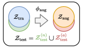
Figure 2: Illustration of $\mathcal{L}_{\mathrm{val}}$.

The unsupervised validation loss $\mathcal{L}_{\mathrm{val}}$ is one of the core components of ST-SSAD, which guides the direction of hyperparameter optimization. The main goal of $\mathcal{L}_{\mathrm{val}}$ is to quantify the agreement between the augmentation $\phi_{\mathrm{aug}}$ and the anomaly-generating mechanism yielding $\mathcal{D}_{\mathrm{test}}$ without labels. Our idea is to measure the distance between $\mathcal{D}_{\mathrm{trn}}\cup\mathcal{D}_{\mathrm{aug}}$ and $\mathcal{D}_{\mathrm{test}}$ in the embedding space, based on the intuition that the two sets will become similar, the more $\mathcal{D}_{\mathrm{aug}}$ resembles the true anomalies in $\mathcal{D}_{\mathrm{test}}$. Fig. 2 illustrates the intuition: we aim to find $\phi_{\mathrm{aug}}$ that creates $\mathcal{Z}_{\mathrm{aug}}$ similar to the set $\mathcal{Z}_{\mathrm{test}}^{{\scriptscriptstyle(}a{\scriptscriptstyle)}}$ of true anomalies (in red), while matching $\mathcal{Z}_{\mathrm{trn}}$ with the set $\mathcal{Z}_{\mathrm{test}}^{{\scriptscriptstyle(}n{\scriptscriptstyle)}}$ of normal data in $\mathcal{D}_{\mathrm{test}}$ (in green). By using the embeddings, we can effectively avoid the high dimensionality of raw data and focus on their semantic representation.

Based on the idea, we present the basic form of our validation loss as follows:

$$\smash{\mathcal{L}_{\mathrm{val}}^{(b)}}(\mathcal{Z}_{\mathrm{trn}},\mathcal{Z}_{\mathrm{aug}},\mathcal{Z}_{\mathrm{test}})=\mathrm{dist}(\mathcal{Z}_{\mathrm{trn}}\cup\mathcal{Z}_{\mathrm{aug}},\mathcal{Z}_{\mathrm{test}}),$$ (1)

where $\mathrm{dist}(\cdot,\cdot)$ is a distance function between sets of vectors. Effectiveness of $\smash{\mathcal{L}_{\mathrm{val}}^{(b)}}$ is determined by how the distance is defined, which we carefully design to address two notable challenges:

1. Scale invariance: The scale of distances between embeddings can arbitrarily change as $\mathbf{a}$ is updated, which makes the value of $\mathcal{L}_{\mathrm{val}}$ inconsistent. Thus, $\mathcal{L}_{\mathrm{val}}$ should be robust to the scale of distances as long as the (relative) distribution of embeddings is preserved.

2. Ratio invariance: Let $\gamma=|\mathcal{D}_{\mathrm{aug}}|/|\mathcal{D}_{\mathrm{trn}}|$ denote the ratio of augmented data, which means the number of times we apply $\phi_{\mathrm{aug}}$ to $\mathcal{D}_{\mathrm{trn}}$. Since the exact anomaly ratio in $\mathcal{D}_{\mathrm{test}}$ is unknown, $\mathcal{L}_{\mathrm{val}}$ should be robust to the value of $\gamma$ which we manually set prior to training.

Algorithm 1 ST-SSAD: Self-Tuning Self-Supervised Anomaly Detection

1:Training data $\mathcal{D}_{\mathrm{trn}}$, test data $\mathcal{D}_{\mathrm{test}}$, augmentation function $\phi_{\mathrm{aug}}$, training loss $\mathcal{L}_{\mathrm{trn}}$, validation loss $\mathcal{L}_{\mathrm{val}}$, detector $f_{\theta}$ with parameters $\theta$, number of epochs $T$, and step sizes $\alpha$ and $\beta$

2:Optimized augmentation hyperparameters $\mathbf{a}^{(T)}$

3:$\mathbf{a}^{(0)}\leftarrow$ Initialize augmentation hyperparameters

4:for $t\in\{0,1,\cdots,T-1\}$ do

5:    Let $\theta^{\prime}=\theta-\alpha\nabla_{\theta}\mathcal{L}_{\mathrm{trn}}(\theta,\mathbf{a}^{(t)})$ $\triangleright$ Get new parameters as a function of $\mathbf{a}^{(t)}$

6:    $\mathcal{Z}_{\mathrm{trn}}\leftarrow\{f_{\theta^{\prime}}(\mathbf{x})\mid\mathbf{x}\in\mathcal{D}_{\mathrm{trn}}\}$ $\triangleright$ Generate training embeddings

7:    $\mathcal{Z}_{\mathrm{aug}}\leftarrow\{f_{\theta^{\prime}}(\phi_{\mathrm{aug}}(\mathbf{x};\mathbf{a}^{(t)}))\mid\mathbf{x}\in\mathcal{D}_{\mathrm{trn}}\}$ $\triangleright$ Generate augmented embeddings

8:    $\mathcal{Z}_{\mathrm{test}}\leftarrow\{f_{\theta^{\prime}}(\mathbf{x})\mid\mathbf{x}\in\mathcal{D}_{\mathrm{test}}\}$ $\triangleright$ Generate test embeddings

9:    $\mathcal{Z}_{\mathrm{trn}},\mathcal{Z}_{\mathrm{aug}},\mathcal{Z}_{\mathrm{test}}\leftarrow\mathrm{normalize}(\mathcal{Z}_{\mathrm{trn}},\mathcal{Z}_{\mathrm{aug}},\mathcal{Z}_{\mathrm{test}})$ $\triangleright$ Normalize embeddings as in Eq. (2)

10:    $\mathbf{a}^{(t+1)}\leftarrow\mathbf{a}^{(t)}-\beta\nabla_{\mathbf{a}}\mathcal{L}_{\mathrm{val}}(\mathcal{Z}_{\mathrm{trn}},\mathcal{Z}_{\mathrm{aug}},\mathcal{Z}_{\mathrm{test}})$ $\triangleright$ Update the augmentation hyperparameters

11:    $\theta\leftarrow\theta^{\prime}$ $\triangleright$ Update the detector network parameters

12:end for

Total distance normalization    For scale invariance, we propose total distance normalization to unify the total pairwise squared distance (TPSD) [19] of embeddings. Let $\mathbf{Z}$ be an embedding matrix that concatenates all embedding vectors in $\mathcal{Z}_{\mathrm{trn}}$, $\mathcal{Z}_{\mathrm{aug}}$, and $\mathcal{Z}_{\mathrm{test}}$. Then, TPSD is defined as $\mathrm{TPSD}(\mathbf{Z})=\sum_{ij}\|\mathbf{z}_{i}-\mathbf{z}_{j}\|_{2}^{2}$, where $\mathbf{z}_{i}$ denotes the $i$-th row of $\mathbf{Z}$. Although the naïve computation of TPSD is slow, we can transform any $\mathbf{Z}$ to have the unit TPSD in linear time [19] via

$$\mathbf{z}_{i}^{\prime}=\frac{\sqrt{N}}{\|\mathbf{Z}^{c}\|_{\mathrm{F}}}\mathbf{z}_{i}^{c}\quad\textrm{where}\quad\mathbf{z}_{i}^{c}=\mathbf{z}-\frac{1}{N}\sum_{i=1}^{N}\mathbf{z}_{i}\;,$$ (2)

where $\|\cdot\|_{\mathrm{F}}$ is the Frobenius norm of a matrix, and $N$ is the number of rows in $\mathbf{Z}$.

By using $\mathbf{Z}^{\prime}$ instead of $\mathbf{Z}$ for computing the distances, we can focus on the relative distances between embeddings while maintaining the overall variance. It is noteworthy that the vector normalization, i.e., $\mathbf{z}_{i}\leftarrow\mathbf{z}_{i}/\|\mathbf{z}_{i}\|_{2}\ \forall i$, does not solve the problem since the scale of distances can still be arbitrary even with the upper bound of individual distances forced by the unit vectors. Another advantage that total distance normalization offers is that it steers away from the trivial solution of the distance minimization problem, which is to set all embeddings to the zero vector.

Mean distance loss    For ratio invariance, we use the asymmetric mean distance as the $\mathrm{dist}$ function to separate $\mathrm{dist}(\mathcal{Z}_{\mathrm{trn}}\cup\mathcal{Z}_{\mathrm{aug}},\mathcal{Z}_{\mathrm{test}})$ into $(\mathrm{dist}(\mathcal{Z}_{\mathrm{trn}},\mathcal{Z}_{\mathrm{test}})+\mathrm{dist}(\mathcal{Z}_{\mathrm{aug}},\mathcal{Z}_{\mathrm{test}}))/2$ as follows.

$$\mathcal{L}_{\mathrm{val}}(\mathcal{Z}_{\mathrm{trn}},\mathcal{Z}_{\mathrm{aug}},\mathcal{Z}_{\mathrm{test}})=\frac{1}{2}\sum_{\mathbf{z}^{\prime}\in\mathcal{Z}_{\mathrm{test}}^{\prime}}\|\mathbf{z}^{\prime}-\mathrm{mean}(\mathcal{Z}_{\mathrm{trn}}^{\prime})\|_{2}+\|\mathbf{z}^{\prime}-\mathrm{mean}(\mathcal{Z}_{\mathrm{aug}}^{\prime})\|_{2}\;,$$ (3)

where $\mathcal{Z}_{\mathrm{trn}}^{\prime}$, $\mathcal{Z}_{\mathrm{aug}}^{\prime}$, and $\mathcal{Z}_{\mathrm{test}}^{\prime}$ are the embeddings after the total distance normalization, and $\mathrm{mean}(\cdot)$ is the (elementwise) mean of a set of vectors. The mean operation allows $\mathcal{L}_{\mathrm{val}}$ to be invariant to the individual (or internal) distributions of $\mathcal{Z}_{\mathrm{trn}}$ and $\mathcal{Z}_{\mathrm{aug}}$, including their sizes, while focusing on their global relative positions with respect to the test embeddings in $\mathcal{Z}_{\mathrm{test}}$. This is another desired property for $\mathcal{L}_{\mathrm{val}}$, since we want to avoid minimizing $\mathcal{L}_{\mathrm{val}}$ only by decreasing the variance of $\mathcal{Z}_{\mathrm{aug}}$. More detailed discussion on the properties of $\mathcal{L}_{\mathrm{val}}$ under various scenarios is given in Appendix A.

3.2 Differentiable Augmentation

The second driving engine is a differentiable augmentation function that enables ST-SSAD to conduct end-to-end optimization. There are two main approaches to making augmentation differentiable. The first is to train a neural network that mimics the augmentation function, mapping input samples to augmented counterparts, which can be done offline regardless of the detector network $f_{\theta}$. However, such a neural network is required to have a large capacity to be able to learn the augmentation function accurately, especially for high dimensional target samples, which demands considerable training cost.

The second approach is to directly formulate an augmentation function in a differentiable way. Some functions are inherently differentiable if implemented in a correct way, while others require differentiable surrogate functions that provide a similar functionality. As proof of concept, we take this approach to introduce two differentiable augmentation functions; one representative of local and another representative of global augmentation. Specifically, we propose the novel CutDiff (§3.2.1) as a differentiable variant of CutOut [18] that is originally designed for localized anomalies. We also utilize a differentiable formulation of Rotation (§3.2.2), which is a popular augmentation that transforms the input globally and has been widely used for semantic anomaly detection [8, 10, 12].

3.2.1 CutDiff for Local Augmentation

Algorithm 2 Proposed CutDiff Augmentation

1:Image $\mathbf{x}$ and augmentation hyperparameters $\mathbf{a}\in\mathbb{R}^{3}$

2:Augmented image $\tilde{\mathbf{x}}$

3:$\mathbf{X}\leftarrow$ Reshape $\mathbf{x}$ as a tensor of size $m\times m\times 3$, assuming an RGB image

4:$\mathbf{L}\leftarrow$ Reshape $\mathbf{a}$ as a lower triangular matrix of size $2\times 2$

5:$\mathbf{G}\leftarrow$ Create a grid tensor of size $m\times m\times 2$ such that $\mathbf{g}_{ij}=(i/m,j/m)\ \forall i,j\in[1,m]$

6:$\bm{\mu}\leftarrow$ Sample a position vector of size $2$ such that $\mu_{1},\mu_{2}\sim\mathrm{uniform}(0,1)$

7:$\mathbf{P}\leftarrow$ Create a patch matrix such that $p_{ij}=\exp(-(\mathbf{g}_{ij}-\bm{\mu})^{\top}(\mathbf{L}\mathbf{L}^{\top})^{-1}(\mathbf{g}_{ij}-\bm{\mu}))$

8:$\tilde{\mathbf{x}}\leftarrow$ Reshape $\tilde{\mathbf{X}}$ where $\tilde{x}_{ijk}=\min(\max(x_{ijk}-p_{ij},0),1)\ \forall i,j,k$

Local augmentation functions such as CutOut [18], CutPaste [11], and patch-wise cloning [20] mimic subtle local anomalies such as textural defects by modifying a partial region in an image. CutOut removes a small patch from an image and fills in it with a black patch, while CutPaste copies a small patch and pastes it into a different random location of the same image. However, all of these functions are not differentiable, and thus cannot be directly used for our end-to-end ST-SSAD framework.

We propose CutDiff in Algo. 2, which creates a smooth round patch and extracts it from the given image in a differentiable manner. The main idea is to model the shape of the patch as a function of hyperparameters $\mathbf{a}\in\mathbb{R}^{3}$ by computing the scaled distance between each image pixel and the randomly selected center of the patch. The three elements in $\mathbf{a}$ represent the patch shape including its width, height, and orientation. Let $\mathbf{R}$ and $\mathbf{S}$ respectively denote the rotation and scale matrices for a patch, as $\mathbf{R}=\left[\begin{matrix}\cos(g)&-\sin(g)\\ \sin(g)&\cos(g)\end{matrix}\right]{\;\;\;\text{and}\;\;\;}\mathbf{S}=\left[\begin{matrix}s/r&0\\ 0&sr\end{matrix}\right]$, where $g$, $s$, and $r$ represent the rotated angle, size, and ratio, respectively. These three elements can be associated with those in $\mathbf{a}$ through $\mathbf{L}=\mathbf{R}\mathbf{S}$, where $\mathbf{L}$ is a lower triangular matrix of $\mathbf{a}$ as given in Line 2 of Algo. 2. By directly learning $\mathbf{L}$, we in effect tune the rotation and scale of the patch. We provide visualization of CutDiff compared with CutOut and CutPaste, as well as implementation details in Appendix B.

3.2.2 Rotation for Global Augmentation

Geometric augmentation functions such as rotation, translation, and flipping have been widely used for image anomaly detection [8, 10]. Unlike the local augmentation functions such as CutOut, many geometric transformations are differentiable as they are represented by matrix-vector operations. In this work, we use the differentiable image rotation function proposed by Jaderberg et al. [21], which consists of two main steps. First step is the creation of a rotation matrix, which is the same as the $\mathbf{R}$ matrix except that zeros are padded as the third column. Second step is to create a sampling function that selects a proper pixel position from the given image for each pixel position of the target image based on the computed rotation matrix and the affine grid. The resulting operation is differentiable, since it is a mapping from the original pixels to the output through a parameterized sampling.

3.3 Implementation Details

Second-order optimization    ST-SSAD updates augmentation hyperparameters $\mathbf{a}$ and the parameters $\theta$ of the detection network $f_{\theta}$ through alternating stages at each training iteration. That is, we expect the following to hold:

$$\mathcal{L}_{\mathrm{val}}(\mathbf{a}^{(t+1)},\theta^{\prime})\;<\;\mathcal{L}_{\mathrm{val}}(\mathbf{a}^{(t)},\theta)\;,$$ (4)

where $t$ is the current number of epochs, and $\theta^{\prime}$ denotes the updated parameters of the detector $f_{\theta}$ derived by using $\smash{\mathbf{a}^{(t)}}$ to generate pseudo anomalies for its training.

However, the first-order optimization of $\mathbf{a}$ cannot take into account that the parameters $\theta^{\prime}$ and $\theta$ are different between both sides of Eq. (4), as it treats $\theta^{\prime}$ as a constant. As a solution, ST-SSAD considers $\theta^{\prime}$ as a function of $\mathbf{a}^{(t)}$ and conducts second-order optimization as follows:

$$\mathbf{a}^{(t+1)}=\mathbf{a}^{(t)}-\beta\nabla_{\mathbf{a}^{(t)}}\mathcal{L}_{\mathrm{val}}(\mathbf{a}^{(t)},\theta-\alpha\nabla_{\theta}\mathcal{L}_{\mathrm{trn}}(\theta,\mathbf{a}^{(t)}))\;.$$ (5)

In this way, the optimization process can accurately track the change in $\theta$ caused by the update of $\mathbf{a}$, resulting in a stable minimization of $\mathcal{L}_{\mathrm{val}}$. Note that Eq. (5) is the same as in Line 8 of Algorithm 1, except we assume that $\mathcal{L}_{\mathrm{val}}$ takes $(\mathbf{a},\theta)$ as its inputs in Eq.s (4) and (5).

Initialization    The result of ST-SSAD is affected by the initialization of augmentation hyperparameters $\mathbf{a}$, since it conducts gradient-based updates toward local optima. A natural way to address initialization is to pick a few random starting points and select the best one. However, it is difficult to fairly select the best from multiple initialization choices, since our $\mathcal{L}_{\mathrm{val}}$ is designed to locally improve the current $\mathbf{a}$, rather than to compare different models; e.g., it is possible that a less-aligned model can produce lower $\mathcal{L}_{\mathrm{val}}$ if the augmented data are distributed more sparsely in the embedding space.

As a solution, we propose a simple yet effective measure to enable the comparison between models from different initialization points. Let $s$ denote the anomaly score function as presented in the problem definition in Sec. 2. Then, we define the score variance of the test data as

$$\mathcal{S}(\theta)=\frac{\sum_{s\in\mathcal{C}}(s-\mathrm{mean}(\mathcal{C}))^{2}}{|\mathcal{D}_{\mathrm{test}}|-1}\textrm{ \;\; where \;\; }\mathcal{C}=\{s(f_{\theta}(\mathbf{x}))\mid\mathbf{x}\in\mathcal{D}_{\mathrm{test}}\}.$$ (6)

We use $\mathcal{S}$ (the larger, the better) to select the best initialization point after training completes. The idea is that the variance of test anomaly scores is likely to be large under a good augmentation, as it generally reflects a better separability between inliers and anomalies in the test data, and it offers a fair evaluation since ST-SSAD does not observe the score function $s$ at all during optimization.

4 Experiments

Datasets    We evaluate ST-SSAD on 41 different anomaly detection tasks, which include 23 subtle (local) anomalies in MVTec AD [22] and 18 semantic (gross) anomalies in SVHN [23]. MVTec AD is an image dataset of industrial objects, where the anomalies are local defects such as scratches. We use four types of objects in our experiments: Cable, Carpet, Grid, and Tile, each of which contains five to eight anomaly types. SVHN is a digits image dataset from house numbers in Google Street View. We use digits 2 and 6 as normal classes and treat the remaining digits as anomalies, generating 18 different anomaly detection tasks for all pairs of digits (2 vs. others and 6 vs. others).

Model settings    We use a detector network $f_{\theta}$ based on ResNet-18 [24] that was used in previous work for unsupervised anomaly detection [11]. We use the binary cross entropy as the training loss $\mathcal{L}_{\mathrm{trn}}$ for classifying between normal and augmented data, applying an MLP head to the embeddings to produce prediction outputs. The anomaly score $s(\textbf{x})$ of each data $\mathbf{x}$ is defined as the negative log likelihood of a Gaussian density estimator learned on the embeddings of training data as in previous works [25, 11]. For ST-SSAD, we use four uniformly sampled initializations for each augmentation function: $\{0.0001,0.001,0.01,0.1\}$ for CutDiff patch size, and $\{45^{\circ},135^{\circ},225^{\circ},315^{\circ}\}$ for Rotation angle. We set both the initial patch angle and ratio to zero. We employ CutDiff and Rotation for defect and semantic anomaly detection tasks, respectively. The sum of training and validation losses is used as the stopping criterion for the updates to hyperparameters $\mathbf{a}$.

Evaluation metrics    The accuracy of each model is measured by the area under the ROC curve (AUC) on the anomaly scores computed for $\mathcal{D}_{\mathrm{test}}$. We run all experiments 5 times and report the average and standard deviation. For statistical comparison between different models on all tasks and random seeds, we also run the paired Wilcoxon signed-rank test [26]. The one-sided test with $p$-values smaller than $0.05$ represents that our ST-SSAD is statistically better than the other.

Baselines    To the best of our knowledge, there are no direct competitors on augmentation hyperparameter tuning for self-supervised anomaly detection. Thus, we compare ST-SSAD with various types of baselines: SSL without hyperparameter tuning—(1) random dynamic selection (RD) that selects $\mathbf{a}$ randomly at each training epoch, and (2) random static selection (RS) that selects $\mathbf{a}$ once before the training begins. Unsupervised learning—(3) autoencoder (AE) [8] and (4) DeepSVDD [27]. Variants of our ST-SSAD with naïve choices—(5) using maximum mean discrepancy (MMD) [28] as $\mathcal{L}_{\mathrm{val}}$, (6) MMD without the total distance normalization, and (7) using first-order optimization. RD and RS are used with either of CutOut, CutPaste, CutDiff, or Rotation, which we denote CO, CP, CD, and RO for brevity. We also depict baselines (5)–(7) as MMD1, MMD2, and FO, respectively. Additional details on experiments are given in Appendix C.

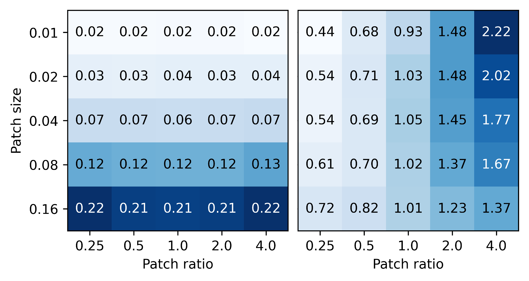
(a) Learned values of patch size (left) & ratio (right)

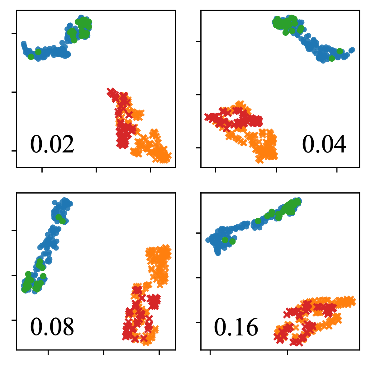
(b) $t$-SNE embeddings

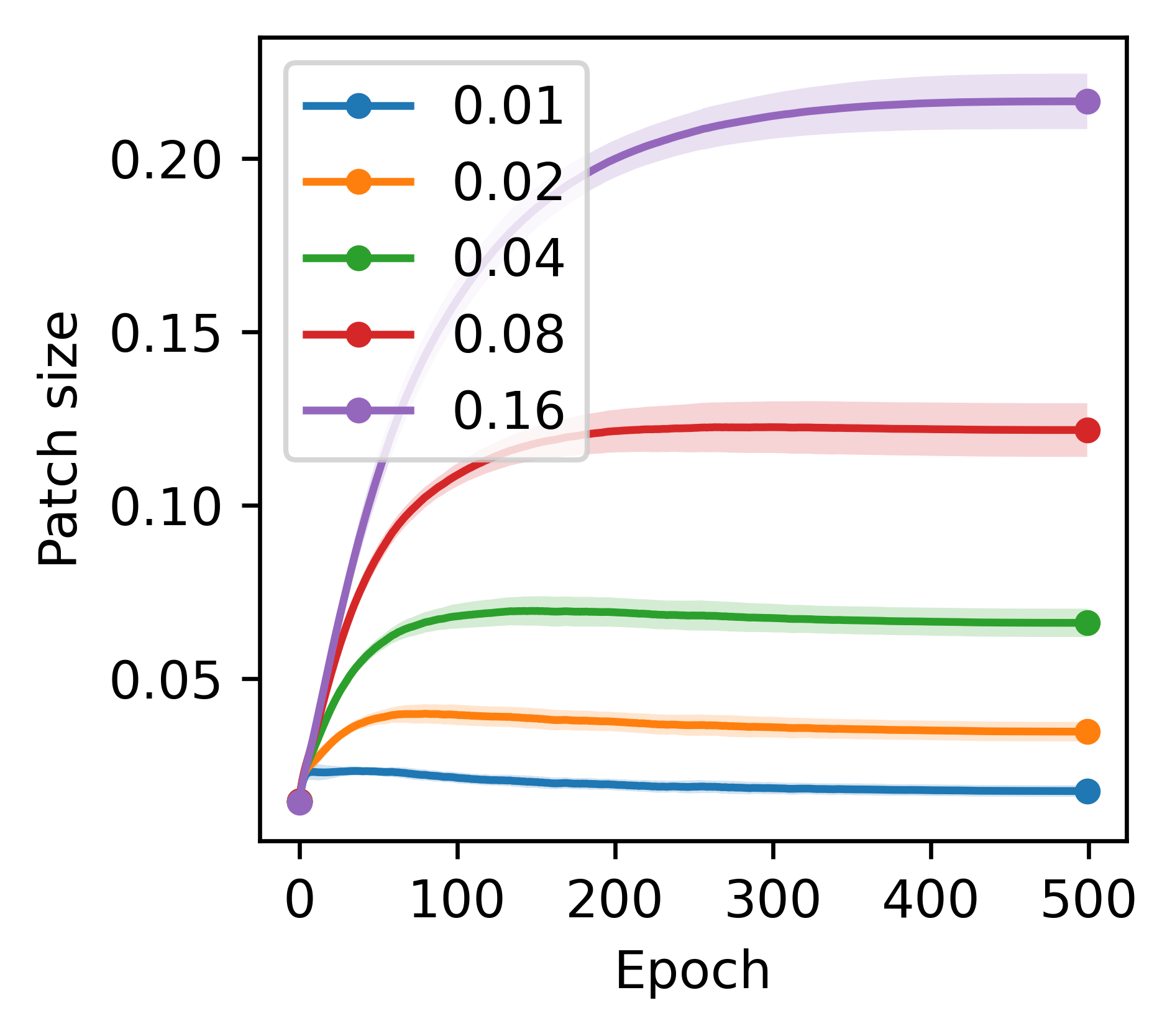
(c) Patch size during training

Figure 3: Experimental results on demonstrative examples, where we create anomalies using CutDiff with different hyperparameters. (a) ST-SSAD learns $\mathbf{a}$ differently for each anomaly type, following the true values shown in the $x$- and $y$-axes, until (b) the embedding distributions are matched between $\mathcal{Z}_{\mathrm{trn}}\cup\mathcal{Z}_{\mathrm{aug}}$ and $\mathcal{Z}_{\mathrm{test}}$, showing a learning trajectory like (c). AUC is $1.00$ in all 25 tasks.

4.1 Demonstrative Examples

We first present experimental results on demonstrative datasets, where we create anomalies using CutDiff with different augmentation hyperparameters. Specifically, given images of the Carpet object in MVTec AD, we create 25 types of anomalies with the patch size in $\{0.01,0.02,0.04,0.08,0.16\}$ and the aspect ratio in $\{0.25,0.5,1.0,2.0,4.0\}$, where the angle is fixed to $0$. Our goal is to demonstrate that ST-SSAD is able to learn different $\mathbf{a}$ for different anomaly types in these controlled settings.

Fig. 3 shows the results of learning. In Fig. 3(a), ST-SSAD learns different values of $\mathbf{a}$ depending on the properties of anomalies, demonstrating the ability of ST-SSAD to adapt to varying anomalies. Nevertheless, there exists slight difference between the learned $\mathbf{a}$ and the true values in some cases, as embedding distributions can be matched as in Fig. 3(b) even with such a difference. This difference is typically larger for patch ratio than for patch size, suggesting that patch size impacts the embeddings more than the ratio does. Fig. 3(c) depicts the training process of ST-SSAD for five anomaly types with different patch sizes, where the patch ratio is $1.0$. We visualize the average and standard deviation from five runs with different random seeds. ST-SSAD accurately adapts to different patch sizes even from the same initialization point, updating $\mathbf{a}$ through iterations to minimize the validation loss.

4.2 Testbed Evaluation

Next, we perform quantitative evaluation of ST-SSAD on both industrial-defect anomalies and semantic class anomalies, covering 41 different anomaly detection tasks. Table 1 provides the results on 23 tasks for industrial-defect anomalies. ST-SSAD achieves the best AUC in 9 different tasks, and it outperforms 7 baselines with most $p$-values smaller than $0.01$, representing strong statistical significance. Table 2 shows the results on 18 detection tasks for semantic class anomalies, where ST-SSAD significantly outperforms all baselines with all $p$-values smaller than $0.0001$.

The ablation studies between ST-SSAD and its three variants in Tables 1 and 2 show the effectiveness of our ideas that compose ST-SSAD: total distance normalization, mean distance loss, and second-order optimization. Especially, the two MMD-based models are significantly worse than our ST-SSAD, showing that MMD is not suitable for augmentation tuning even though it is widely used as a set distance measure, due to the challenges we aim to address with $\mathcal{L}_{\mathrm{val}}$. The difference between ST-SSAD and the first-order baseline is smaller, meaning that the first-order optimization can still be used for ST-SSAD when the computational efficiency needs to be prioritized.

Table 1: Test AUC on 23 different tasks for subtle anomaly detection. Each number is the average from five runs, and the best in each row is in bold. ST-SSAD outperforms most baselines, which is supported by the $p$-values in the last row derived from the Wilcoxon signed rank test.

Main Result											Ablation Study
Object	Anomaly Type	AE	D-SVDD	RS-CO	RD-CO	RS-CP	RD-CP	RS-CD	RD-CD	ST-SSAD	MMD1	MMD2	FO
Cable	Bent wire	0.515	0.432	0.556	0.560	0.703	0.756	0.527	0.580	0.490	0.581	0.643	0.579
Cable	Cable swap	0.639	0.295	0.483	0.625	0.618	0.683	0.574	0.696	0.532	0.510	0.562	0.545
Cable	Combined	0.584	0.587	0.879	0.857	0.880	0.949	0.901	0.879	0.925	0.939	0.962	0.882
Cable	Cut inner insulation	0.758	0.591	0.630	0.737	0.766	0.833	0.623	0.732	0.667	0.633	0.649	0.689
Cable	Cut outer insulation	0.989	0.343	0.695	0.815	0.787	0.871	0.703	0.790	0.516	0.428	0.461	0.527
Cable	Missing cable	0.920	0.466	0.953	0.961	0.755	0.801	0.935	0.945	0.998	0.855	0.772	0.999
Cable	Missing wire	0.433	0.494	0.781	0.655	0.501	0.546	0.708	0.620	0.863	0.547	0.477	0.699
Cable	Poke insulation	0.287	0.471	0.469	0.527	0.645	0.672	0.489	0.503	0.630	0.692	0.816	0.676
Carpet	Color	0.578	0.716	0.669	0.508	0.412	0.287	0.643	0.639	0.938	0.761	0.741	0.918
Carpet	Cut	0.198	0.758	0.439	0.608	0.403	0.411	0.490	0.767	0.790	0.353	0.401	0.595
Carpet	Hole	0.626	0.676	0.379	0.613	0.404	0.389	0.470	0.765	0.590	0.438	0.229	0.630
Carpet	Metal contamination	0.056	0.739	0.198	0.304	0.240	0.167	0.255	0.474	0.076	0.392	0.134	0.392
Carpet	Thread	0.394	0.742	0.494	0.585	0.469	0.517	0.508	0.679	0.483	0.492	0.541	0.642
Grid	Bent	0.849	0.168	0.456	0.322	0.421	0.433	0.337	0.354	0.771	0.780	0.650	0.602
Grid	Broken	0.806	0.183	0.397	0.312	0.487	0.502	0.340	0.392	0.869	0.845	0.887	0.884
Grid	Glue	0.704	0.143	0.634	0.568	0.674	0.732	0.681	0.578	0.906	0.966	0.974	0.721
Grid	Metal contamination	0.851	0.229	0.421	0.380	0.499	0.514	0.425	0.613	0.858	0.861	0.665	0.732
Grid	Thread	0.583	0.209	0.612	0.494	0.500	0.549	0.654	0.611	0.973	0.962	0.969	0.964
Tile	Crack	0.770	0.728	0.872	0.993	0.743	0.636	0.837	0.999	0.749	0.740	0.820	0.595
Tile	Glue strip	0.697	0.509	0.693	0.836	0.665	0.700	0.675	0.831	0.767	0.585	0.649	0.561
Tile	Gray stroke	0.637	0.785	0.845	0.642	0.583	0.657	0.856	0.802	0.974	0.653	0.706	0.973
Tile	Oil	0.414	0.690	0.708	0.745	0.464	0.576	0.683	0.837	0.554	0.548	0.614	0.555
Tile	Rough	0.724	0.387	0.606	0.725	0.631	0.661	0.568	0.657	0.690	0.700	0.549	0.605
$p$-value		.0000	.0000	.0000	.0012	.0000	.0000	.0000	.0728	Ours	.0268	.0073	.1332

Table 2: Test AUC on 18 different tasks for semantic anomaly detection. The format is the same as in Table 1. ST-SSAD outperforms all baselines with the $p$-values smaller than $0.0001$ in all cases.

Main Result							Ablation Study
Object	Anomaly	AE	D-SVDD	RS-RO	RD-RO	ST-SSAD	MMD1	MMD2	FO
Digit 2	Digit 0	0.602	0.472	0.672	0.734	0.816	0.519	0.518	0.506
Digit 2	Digit 1	0.544	0.499	0.601	0.609	0.743	0.499	0.501	0.498
Digit 2	Digit 3	0.604	0.503	0.664	0.730	0.832	0.508	0.510	0.511
Digit 2	Digit 4	0.561	0.511	0.679	0.746	0.790	0.531	0.530	0.530
Digit 2	Digit 5	0.625	0.502	0.709	0.824	0.877	0.512	0.514	0.517
Digit 2	Digit 6	0.616	0.496	0.726	0.826	0.887	0.511	0.507	0.510
Digit 2	Digit 7	0.541	0.496	0.584	0.639	0.823	0.521	0.520	0.518
Digit 2	Digit 8	0.616	0.498	0.673	0.738	0.805	0.524	0.524	0.522
Digit 2	Digit 9	0.588	0.485	0.625	0.687	0.659	0.516	0.523	0.518
Digit 6	Digit 0	0.531	0.480	0.586	0.606	0.777	0.503	0.514	0.504
Digit 6	Digit 1	0.517	0.498	0.621	0.610	0.854	0.516	0.528	0.511
Digit 6	Digit 2	0.594	0.503	0.735	0.807	0.916	0.525	0.531	0.529
Digit 6	Digit 3	0.570	0.507	0.686	0.750	0.823	0.518	0.520	0.521
Digit 6	Digit 4	0.525	0.508	0.659	0.703	0.709	0.527	0.521	0.530
Digit 6	Digit 5	0.544	0.502	0.615	0.661	0.658	0.516	0.513	0.509
Digit 6	Digit 7	0.567	0.505	0.699	0.729	0.861	0.540	0.551	0.541
Digit 6	Digit 8	0.546	0.500	0.575	0.641	0.732	0.512	0.523	0.512
Digit 6	Digit 9	0.579	0.495	0.708	0.817	0.944	0.527	0.519	0.524
$p$-value		.0000	.0000	.0000	.0000	Ours	.0000	.0000	.0000

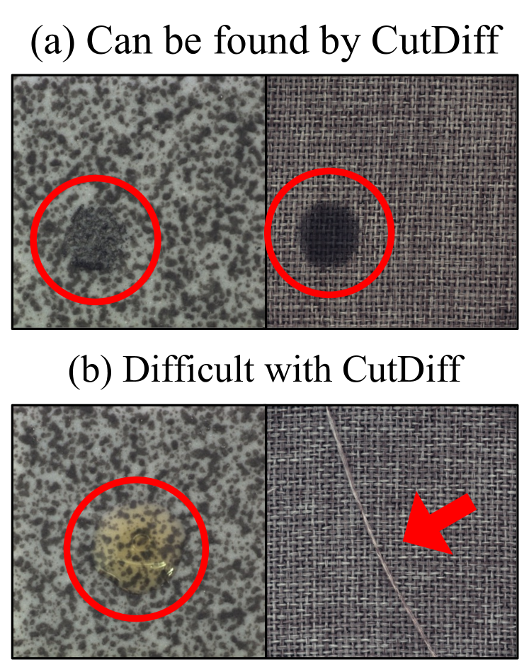
Figure 4: Some anomaly types are hard to detect with CutDiff. See Sec. 4.4 for discussion.

4.3 Qualitative Analysis

We also perform qualitative analysis as shown in Fig.s 5 and 6, visualizing the augmentation functions learned by ST-SSAD for different types of anomalies. Fig. 5 illustrates three types of anomalies in the Cable object and one type of anomaly in the Carpet object. These four anomaly types all have their own sizes and aspect ratios of defected regions, which are accurately learned by ST-SSAD. Note that the three types of Cable anomalies share the training data $\mathcal{D}_{\mathrm{trn}}$; ST-SSAD captures their difference only from the unlabeled test data. The locations of patches created by CutDiff are chosen randomly at each run, since the locations of local defects are different for each anomalous image.

Fig. 6 illustrates images in the SVHN dataset and the embedding distributions after the training of ST-SSAD is completed. Fig.s 6a and 6c show that ST-SSAD learns $180^{\circ}$ as the angle of Rotation, since the anomalies in both tasks can be resembled by the $180^{\circ}$-rotated normal images. After the training is done, the embedding distributions between $\mathcal{Z}_{\mathrm{trn}}\cup\mathcal{Z}_{\mathrm{aug}}$ and $\mathcal{Z}_{\mathrm{test}}$ are matched as shown in Fig.s 6b and 6d, achieving high average AUC of $0.944$ and $0.887$, respectively (see Table 2).

4.4 Discussion

As Table 1 shows, ST-SSAD cannot always improve detection across tasks. In some tasks like Rough anomalies in Tile, a simple baseline like random CutOut shows higher AUC than other models. This is because some anomaly types are hard to mimic with CutDiff due to the inherent mismatch of the augmentation function. Fig. 4 shows two example anomaly types, Tile-Oil and Carpet-Thread, where ST-SSAD cannot improve over the baselines. Local defects of Oil are brighter than the background, whereas CutDiff rather darkens the chosen patch. Anomalies of Thread type contain long thin threads, which are also hard to represent with CutDiff regardless of hyperparameter values.

As a general framework, the performance of ST-SSAD is affected by the detector model and augmentation function used. As the first systematic study for unsupervised augmentation tuning, we propose two differentiable augmentation functions for local and semantic anomalies, respectively, and show the success of ST-SSAD on two types of testbeds as proof of concept. We leave it as a future work to design a broader family of differentiable augmentations which can deal with more diverse types of anomalies, that also apply to data modalities other than images.

5 Related Work

Self-supervised learning (SSL) has seen a surge of attention for pre-training foundation models [29], like LLMs that can generate remarkable human-like text [30]. Self-supervised representation learning has also offered astonishing boost to a variety of tasks in NLP, vision, and recommender systems [31]. In fact, SSL has been argued as the key toward “unlocking the dark matter of intelligence” [32].

Self-supervised anomaly detection (SSAD): Most SSL methods can be categorized as generative versus contrastive. Generative SSAD can further be organized based on (denoising) autoencoders [33, 34, 35, 36], adversarial learning [37, 38], as well as flow-based models [39, 40]. Contrastive SSAD, on the other hand, relies on data augmentation that generates pseudo anomalies by transforming inliers, and a supervised loss that is trained to distinguish between inliers and the pseudo anomalies [41]. Many augmentation strategies are designed for contrastive SSAD including geometric [8, 10], localized cut-paste [11], patch-wise cloning [20], masking [42], distribution-shifting transformation [43], and learnable neural network-based transformation [13]. Beyond synthesizing pseudo anomalies via augmentation, outlier exposure augments inlier-only data from external repos [44, 9].

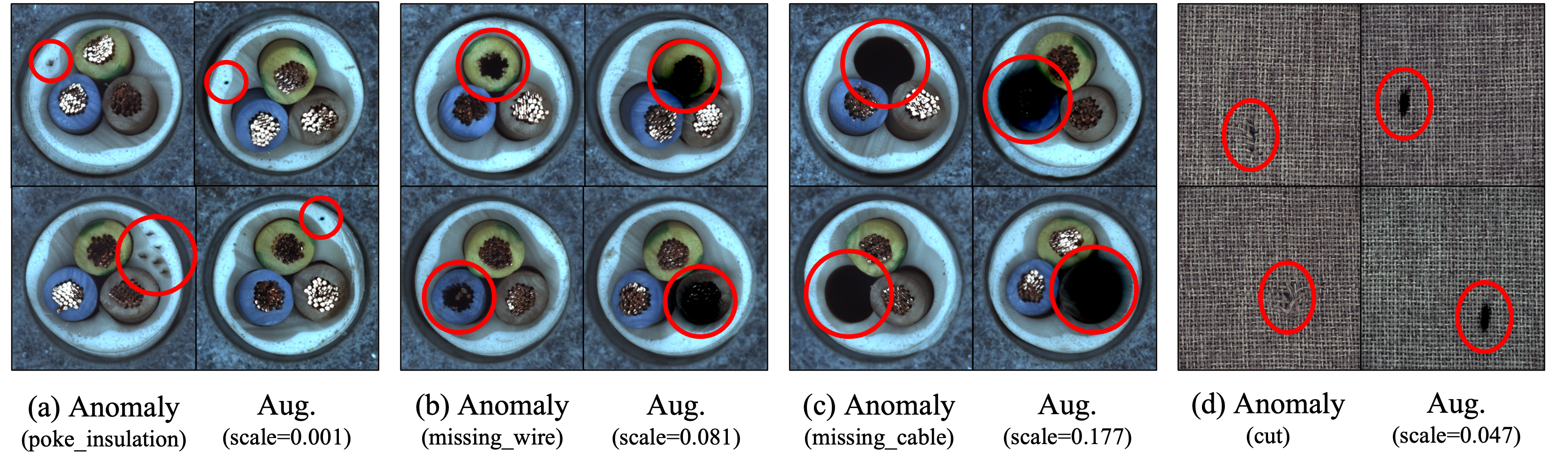
Figure 5: Illustrations of four anomaly types for the Cable and Carpet objects and the corresponding augmentations learned by ST-SSAD. Different hyperparameters of CutDiff are learned to resemble the true anomalies, including both the size and the aspect ratio of a patch.

Figure 6: Illustrations of learned augmentations on the SVHN dataset and the corresponding distributions of embeddings. The three rows in (a, c) represent normal images, augmented images, and anomalies, respectively. ST-SSAD successfully learns the rotation of $180^{\circ}$ for both tasks, achieving a match also visually between the distributions of $\mathcal{Z}_{\mathrm{trn}}\cup\mathcal{Z}_{\mathrm{aug}}$ and $\mathcal{Z}_{\mathrm{test}}$.

Automating augmentation: Recent work in computer vision (CV) have shown that the success of SSL relies heavily on well-designed data augmentation strategies [45, 46]. Sensitivity to the choice of augmentation has also been shown for SSAD recently [14]. While augmentation in CV plays a key role in improving generalization by accounting for invariances (e.g. mirror reflection of a dog is still a dog), augmentation in SSAD plays the key role of presenting the classifier with specific kinds of pseudo anomalies. While the supervised CV community proposed methods toward automating augmentation [15, 47], our proposed work is the first attempt toward rigorously tuning data augmentation for SSAD. The key difference is that the former sets aside a labeled validation set to measure generalization, whereas we address the arguably more challenging setting for fully unsupervised anomaly detection without any labels.

6 Conclusion

Our work presented ST-SSAD, the first framework for self-tuning self-supervised anomaly detection, which automatically tunes the augmentation hyperparameters in an end-to-end fashion. To this end, we addressed two key challenges: unsupervised validation and differentiable augmentation. We proposed a smooth validation loss that quantifies the agreement between augmented and test data in a tranductive fashion. We introduced two differentiable formulations for both local and global augmentation, while ST-SSAD can flexibly accommodate any other differentiable augmentation. Experiments on two large testbeds validated the superiority of ST-SSAD over existing practices. Future work will design differentiable formulations for other augmentation families and then also incorporate the discrete selection of augmentation as part of self-tuning for SSAD.

Appendix A Deeper Analysis on the Validation Loss

A.1 Theoretical Properties on Point Data

We study the theoretical properties of $\mathcal{L}_{\mathrm{val}}$ on simple scenarios, where the embeddings $\mathcal{Z}_{\mathrm{trn}}$, $\mathcal{Z}_{\mathrm{aug}}$, $\mathcal{Z}_{\mathrm{test}}^{{\scriptscriptstyle(}n{\scriptscriptstyle)}}$, and $\mathcal{Z}_{\mathrm{test}}^{{\scriptscriptstyle(}a{\scriptscriptstyle)}}$ are all sets of size one. Lemma 1 shows that $\mathcal{L}_{\mathrm{val}}(\cdot)=1$ when the perfect alignment is achieved, i.e., $\mathcal{Z}_{\mathrm{trn}}\cup\mathcal{Z}_{\mathrm{aug}}=\mathcal{Z}_{\mathrm{test}}$. Lemma 2 shows that $\mathcal{L}_{\mathrm{val}}(\cdot)=1$ is the local minimum which we aim to find through gradient-based optimization (see also Appendix A.2).

Lemma 1.

$\mathcal{L}_{\mathrm{val}}(\mathcal{Z}_{\mathrm{trn}},\mathcal{Z}_{\mathrm{aug}},\mathcal{Z}_{\mathrm{test}})=1$ if $|\mathcal{Z}_{\mathrm{trn}}|=|\mathcal{Z}_{\mathrm{aug}}|=1$, $\mathcal{Z}_{\mathrm{trn}}=\mathcal{Z}_{\mathrm{test}}^{{\scriptscriptstyle(}n{\scriptscriptstyle)}}$, and $\mathcal{Z}_{\mathrm{aug}}=\mathcal{Z}_{\mathrm{test}}^{{\scriptscriptstyle(}a{\scriptscriptstyle)}}$.

Proof.

Let $\mathcal{Z}_{\mathrm{trn}}=\mathcal{Z}_{\mathrm{test}}^{{\scriptscriptstyle(}n{\scriptscriptstyle)}}=\{\mathbf{z}_{1}\}$ and $\mathcal{Z}_{\mathrm{aug}}=\mathcal{Z}_{\mathrm{test}}^{{\scriptscriptstyle(}a{\scriptscriptstyle)}}=\{\mathbf{z}_{2}\}$. Then, the embedding matrix $\mathbf{Z}\in\mathbb{R}^{h\times 4}$ before the total distance normalization is given as

$$\mathbf{Z}=\left[\begin{matrix}\mathbf{z}_{1}&\mathbf{z}_{1}&\mathbf{z}_{2}&\mathbf{z}_{2}\end{matrix}\right].$$

Let $\bar{\mathbf{z}}=(\mathbf{z}_{1}+\mathbf{z}_{2})/2$ be the center of the two vectors, and $\bar{\mathbf{Z}}\in\mathbb{R}^{4\times h}$ be a matrix where each column is $\bar{\mathbf{z}}$. Then, $\mathbf{Z}$ is transformed into $\tilde{\mathbf{Z}}$ as a result of the normalization:

$$\tilde{\mathbf{Z}} =\frac{2}{\sqrt{2\sum_{i}(z_{1i}-\bar{z}_{i})^{2}+2\sum_{i}(z_{2i}-\bar{z}_{i})^{2}}}(\mathbf{Z}-\bar{\mathbf{Z}})$$

$$=\frac{2}{\sqrt{2\sum_{i}((z_{1i}-\bar{z}_{i})^{2}+(z_{2i}-\bar{z}_{i})^{2})}}(\mathbf{Z}-\bar{\mathbf{Z}})$$

$$=\frac{2}{\sqrt{2\sum_{i}((z_{1i}-z_{2i})^{2}/4+(z_{2i}-z_{1i})^{2}/4)}}(\mathbf{Z}-\bar{\mathbf{Z}})$$

$$=\frac{2}{\sqrt{\sum_{i}(z_{1i}-z_{2i})^{2}}}(\mathbf{Z}-\bar{\mathbf{Z}})$$

$$=\frac{2}{\|\mathbf{z}_{1}-\mathbf{z}_{2}\|_{2}}(\mathbf{Z}-\bar{\mathbf{Z}}).$$

The validation loss $\mathcal{L}_{\mathrm{val}}$ is computed on $\tilde{\mathbf{Z}}$ as follows:

$$\mathcal{L}_{\mathrm{val}}(\mathcal{Z}_{\mathrm{trn}},\mathcal{Z}_{\mathrm{aug}},\mathcal{Z}_{\mathrm{test}}) =\frac{1}{4}\left(\|\tilde{\mathbf{z}}_{1}-\tilde{\mathbf{z}}_{1}\|_{2}+\|\tilde{\mathbf{z}}_{1}-\tilde{\mathbf{z}}_{2}\|_{2}+\|\tilde{\mathbf{z}}_{2}-\tilde{\mathbf{z}}_{1}\|_{2}+\|\tilde{\mathbf{z}}_{2}-\tilde{\mathbf{z}}_{2}\|_{2}\right)$$

$$=\frac{1}{2}\|\tilde{\mathbf{z}}_{1}-\tilde{\mathbf{z}}_{2}\|_{2}$$

$$=\frac{1}{2}\left\|\frac{2}{\|\mathbf{z}_{1}-\mathbf{z}_{2}\|_{2}}((\mathbf{z}_{1}-\bar{\mathbf{z}})-(\mathbf{z}_{2}-\bar{\mathbf{z}}))\right\|_{2}$$

$$=1.$$

As a result, the lemma is proved. ∎

Lemma 2.

Assuming that $|\mathcal{Z}_{\mathrm{trn}}|=|\mathcal{Z}_{\mathrm{aug}}|=|\mathcal{Z}_{\mathrm{test}}^{{\scriptscriptstyle(}n{\scriptscriptstyle)}}|=|\mathcal{Z}_{\mathrm{test}}^{{\scriptscriptstyle(}a{\scriptscriptstyle)}}|=1$, let $\mathcal{Z}_{\mathrm{trn}}=\{\mathbf{z}_{1}\}$, $\mathcal{Z}_{\mathrm{aug}}=\{\mathbf{z}_{2}\}$, $\mathcal{Z}_{\mathrm{test}}^{{\scriptscriptstyle(}n{\scriptscriptstyle)}}=\{\mathbf{z}_{1}+\mathbf{u}_{1}\}$, and $\mathcal{Z}_{\mathrm{test}}^{{\scriptscriptstyle(}n{\scriptscriptstyle)}}=\{\mathbf{z}_{2}+\mathbf{u}_{2}\}$, there exists $\delta>0$ that makes $\mathcal{L}_{\mathrm{val}}(\mathcal{Z}_{\mathrm{trn}},\mathcal{Z}_{\mathrm{aug}},\mathcal{Z}_{\mathrm{test}})=1$ if and only if $\mathbf{u}_{1}=\mathbf{u}_{2}=0$ when $\|\mathbf{u}_{1}\|_{2}\leq\delta$ and $\|\mathbf{u}_{2}\|_{2}\leq\delta$.

Proof.

Without loss of generality, we assume the simplest scalar embeddings of size one as $\mathcal{Z}_{\mathrm{trn}}=\{0\}$, $\mathcal{Z}_{\mathrm{test}}^{{\scriptscriptstyle(}n{\scriptscriptstyle)}}=\{u_{1}\}$, $\mathcal{Z}_{\mathrm{aug}}=\{2\}$, $\mathcal{Z}_{\mathrm{test}}^{{\scriptscriptstyle(}a{\scriptscriptstyle)}}=\{u_{2}+2\}$. Then, we show that $\mathcal{L}_{\mathrm{val}}(\mathcal{Z}_{\mathrm{trn}},\mathcal{Z}_{\mathrm{aug}},\mathcal{Z}_{\mathrm{test}})=1$ if and only if $u_{1}=u_{2}=0$ when $\delta=1$. First, we represent the embedding vector (which is used to be a matrix) $\mathbf{z}\in\mathbb{R}^{4}$ before the total distance normalization as

$$\mathbf{z}=(0,u_{1},2,u_{2}+2).$$

Let $\bar{z}=(u_{1}+u_{2}+4)/4$ be the center, and $\bar{\mathbf{z}}\in\mathbb{R}^{4}$ be a vector where each element is $\bar{z}$. Then, $\mathbf{z}$ is transformed into $\tilde{\mathbf{z}}$ as a result of the normalization:

$$\tilde{\mathbf{z}} =\frac{2}{\sqrt{\bar{z}^{2}+(u_{1}-\bar{z})^{2}+(2-\bar{z})^{2}+(u_{2}+2-\bar{z})^{2}}}(\mathbf{z}-\bar{\mathbf{z}})$$

$$=\frac{2}{\sqrt{4\bar{z}^{2}-2(u_{1}+u_{2}+4)\bar{z}+u_{1}^{2}+u_{2}^{2}+4u_{2}+8}}(\mathbf{z}-\bar{\mathbf{z}})$$

$$=\frac{2}{\sqrt{u_{1}^{2}+u_{2}^{2}+4u_{2}+8-4\bar{z}^{2}}}(\mathbf{z}-\bar{\mathbf{z}})$$

$$=\frac{4}{\sqrt{3u_{1}^{2}+3u_{2}^{2}-8u_{1}+8u_{2}-2u_{1}u_{2}+16}}(\mathbf{z}-\bar{\mathbf{z}}).$$

The validation loss $\mathcal{L}_{\mathrm{val}}$ is computed on $\tilde{\mathbf{z}}$ as follows:

$$\mathcal{L}_{\mathrm{val}}(\mathcal{Z}_{\mathrm{trn}},\mathcal{Z}_{\mathrm{aug}},\mathcal{Z}_{\mathrm{test}}) =\frac{|u_{1}|+|u_{1}-2|+|u_{2}|+|u_{2}+2|}{\sqrt{3u_{1}^{2}+3u_{2}^{2}-8u_{1}+8u_{2}-2u_{1}u_{2}+16}}.$$

Then, we can consider four cases based on whether $u_{1}\geq 0$ and $u_{2}\geq 0$. To show that the inequality $\mathcal{L}_{\mathrm{val}}(\mathcal{Z}_{\mathrm{trn}},\mathcal{Z}_{\mathrm{aug}},\mathcal{Z}_{\mathrm{test}})\geq 1$ holds, we represent $\mathcal{L}_{\mathrm{val}}^{2}(\mathcal{Z}_{\mathrm{trn}},\mathcal{Z}_{\mathrm{aug}},\mathcal{Z}_{\mathrm{test}})-1$ as follows:

$$\mathcal{L}_{\mathrm{val}}^{2}(\mathcal{Z}_{\mathrm{trn}},\mathcal{Z}_{\mathrm{aug}},\mathcal{Z}_{\mathrm{test}})-1=\begin{cases}-3u_{1}^{2}+u_{2}^{2}+8u_{1}+8u_{2}+2u_{1}u_{2}&\textrm{if }u_{1}\geq 0\textrm{ and }u_{2}\geq 0\\ -3u_{1}^{2}-3u_{2}^{2}+8u_{1}-8u_{2}+2u_{1}u_{2}&\textrm{if }u_{1}\geq 0\textrm{ and }u_{2}\leq 0\\ u_{1}^{2}+u_{2}^{2}-8u_{1}+8u_{2}-6u_{1}u_{2}&\textrm{if }u_{1}\leq 0\textrm{ and }u_{2}\geq 0\\ u_{1}^{2}-3u_{2}^{2}-8u_{1}-8u_{2}+2u_{1}u_{2}&\textrm{if }u_{1}\leq 0\textrm{ and }u_{2}\leq 0\end{cases}$$

It is straightforward to see that $\mathcal{L}_{\mathrm{val}}^{2}(\mathcal{Z}_{\mathrm{trn}},\mathcal{Z}_{\mathrm{aug}},\mathcal{Z}_{\mathrm{test}})-1\geq 0$ in all four cases if $-1\leq u_{1}\leq 1$ and $-1\leq u_{2}\leq 1$, and the equality holds if and only if $u_{1}=u_{2}=0$. Since $\mathcal{L}_{\mathrm{val}}(\mathcal{Z}_{\mathrm{trn}},\mathcal{Z}_{\mathrm{aug}},\mathcal{Z}_{\mathrm{test}})\geq 0$ by its definition, we prove the lemma for the scalar case. The extension to multi-dimensional cases is trivial, since all operations in $\mathcal{L}_{\mathrm{val}}$ can be generalized to arbitrary dimensions. ∎

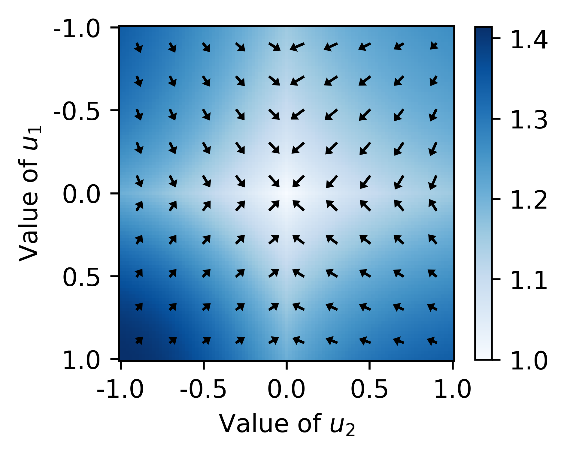
Figure 7: Our validation loss $\mathcal{L}_{\mathrm{val}}$ (as color) for different values of $u_{1}$ and $u_{2}$, which determine the distance between $\mathcal{Z}_{\mathrm{trn}}\cup\mathcal{Z}_{\mathrm{aug}}$ and $\mathcal{Z}_{\mathrm{test}}$, and the negative gradients of $\mathcal{L}_{\mathrm{val}}$ with respect to $u_{1}$ and $u_{2}$ (as arrows). It is satisfied that $\mathcal{Z}_{\mathrm{trn}}\cup\mathcal{Z}_{\mathrm{aug}}=\mathcal{Z}_{\mathrm{test}}$ when $u_{1}=u_{2}=0$. The figure shows that $\mathcal{L}_{\mathrm{val}}$ achieves its minimum when $u_{1}=u_{2}=0$, as claimed in Lemma 2, and the negative gradients consistently point the optimum, supporting the use of gradient-based optimization.

A.2 Demonstrative Example on Point Data

We conduct experiments on actual examples to empirically demonstrate Lemma 2. Assume that every embedding is a scalar, and $\mathcal{Z}_{\mathrm{trn}}=\{0\}$, $\mathcal{Z}_{\mathrm{aug}}=\{2\}$, $\mathcal{Z}_{\mathrm{test}}^{{\scriptscriptstyle(}n{\scriptscriptstyle)}}=\{u_{1}\}$, and $\mathcal{Z}_{\mathrm{test}}^{{\scriptscriptstyle(}a{\scriptscriptstyle)}}=\{u_{2}+2\}$. Our goal is to observe how $\mathcal{L}_{\mathrm{val}}$ changes depending on the values of $u_{1}$ and $u_{2}$, and see if it is minimized only when $u_{1}=u_{2}=0$ as claimed in Lemma 2. Fig. 7 shows how $\mathcal{L}_{\mathrm{val}}$ changes by $u_{1}$ and $u_{2}$. The value of $\mathcal{L}_{\mathrm{val}}$ achieves its minimum when there is the perfect alignment ($u_{1}=u_{2}=0$) in the embedding space. Moreover, the negative gradients with respect to $(u_{1},u_{2})$ denoted as the arrows show that our gradient-based optimization can guide us to the optimum through iterations. This demonstrates that $\mathcal{L}_{\mathrm{val}}$ can effectively measure the semantic alignment in an unsupervised differentiable manner.

Appendix B Detailed Information of CutDiff

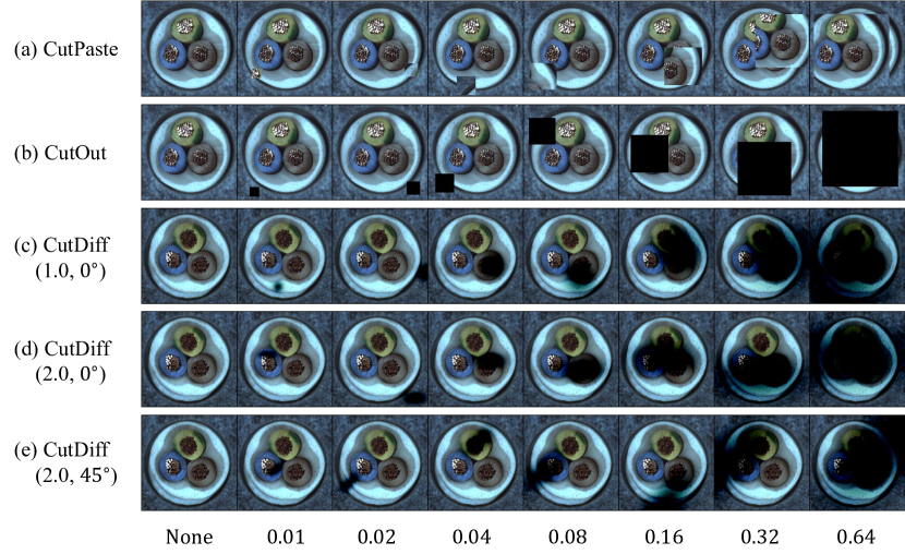
Figure 8: Comparison between three local augmentation functions: (a) CutPaste, (b) CutOut, and (c - e) CutDiff with different hyperparameter choices. Each column represents a different patch size in $[0.01,0.64]$, and the two numbers in (c - e) represent the aspect ratio and the rotated angle of a patch, respectively. CutDiff creates a smooth differentiable boundary unlike the other two functions.

B.1 Visualization with Different Hyperparameters

Fig. 8 shows the images generated from CutPaste, CutOut, and CutDiff, respectively, with different hyperparameter choices. CutDiff is similar to CutOut, except that it generates a smooth circular patch which supports gradient-based updates of its hyperparameters. It is clear from the figure that the two other augmentations, CutPaste and CutOut, are not differentiable as they replace the original pixels with new ones (either black for CutOut or a copied patch for CutPaste).

B.2 Detailed Explanation on the CutDiff Algorithm

We provide more details of CutDiff in Alg. 2 and discuss what makes it differentiable unlike existing augmentation functions like CutOut. Recall that image augmentation is a function of pixel positions, rather than pixel values; although the output is determined also by the input image, the pixel values do not change how the augmentation performs. The main idea of CutDiff is to introduce a grid $\mathbf{G}$ of pixel locations as in Line 3 of Alg. 2 and design a differentiable function that takes $\mathbf{G}$ as an input and determines how to augment each pixel location based on the augmentation hyperparameters $\mathbf{a}$.

The process contains three steps. First, we sample the center position $\mu$ as in Line 4 of Alg. 2, which is a constant with respect to $\mathbf{a}$. Then, for each position $(i,j)$, we determine the amount of change to make with augmentation based on the distance from $\mu$ scaled by $\mathbf{a}$ (in Line 5). In other words, the amount of change is small if $(i,j)$ is far from $\mu$, where the exact value is affected also by $\mathbf{a}$. Lastly, we replace the assignment (or replacement) operation in CutOut (and CutPaste) with the subtract operation (in Line 6). The $\mathrm{min}$ and $\mathrm{max}$ operations are used to ensure that the output pixels are in $[0,1]$. Thanks to the subtraction, the information of the original pixels, not only the pixel locations, is passed to the output image, allowing the gradient to flow to both the given image $\mathbf{x}$ and $\mathbf{a}$.

It is notable that we can also model the patch location $\mu$ as a hyperparameter in $\mathbf{a}$. The problem is that it makes a too strong assumption that a defect is located similarly in all images, which may not be true in many cases. The randomness of $\mu$ does not harm the gradient-based optimization of ST-SSAD, because the validation loss $\mathcal{L}_{\mathrm{val}}$ is computed on a set of embeddings at once, rather than on each individual sample, which may cause the instability of optimization process.

Appendix C Detailed Experimental Setup

C.1 Implementation Details

ST-SSAD has two techniques in its implementation which are not introduced in the main paper due to the lack of space. The first is a warm start, which means that we train the detector $f_{\theta}$ for a fixed number of epochs before starting the alternating updates of $\theta$ and the augmentation hyperparameters $\mathbf{a}$. The warm start is required since the gradient-based update of $\mathbf{a}$ is ineffective if the detector $f_{\theta}$ does not perform well on the current $\mathbf{a}$; in such a case, the validation loss $\mathcal{L}_{\mathrm{val}}$ can have an arbitrary value which is not related to the true alignment of $\mathbf{a}$. The number of training epochs for warm start is chosen to sufficiently minimize the training loss $\mathcal{L}_{\mathrm{trn}}$ for the initial $\mathbf{a}$.

The second technique is to update $\theta$ multiple times for each update of $\mathbf{a}$. This is based on the same motivation as in the first technique; we need to ensure the reasonable performance of $f_{\theta}$ during the iterative updates. The default choice is only one update of $\theta$, but when the training loss $\mathcal{L}_{\mathrm{trn}}$ does not decrease enough at each iteration, one needs to consider increasing the number of updates.

C.2 Hyperparameter Choices

We choose the model and training hyperparameters of ST-SSAD mostly based on a previous work [11], including the detector network $f_{\theta}$ and the score function $s$, and use them across all tasks in our experiments. On the other hand, we tune some of the hyperparameters that affect the effectiveness of training and need to be controlled based on the property of each dataset:

• Batch size: 32 (in MVTecAD) and 256 (in SVHN)

• Number of epochs for warm start: 20 (in MVTecAD) and 40 (in SVHN)

• Number of updates for detector parameters $\theta$: 1 (in MVTec) and 5 (in SVHN)

• Number of maximum iterations: 500 (in MVTecAD) and 100 (in SVHN)

Batch size is set to a small number in MVTecAD, since the images in the dataset have high resolution $256\times 256$, causing high memory cost, while the number of samples is small in both training and test data. The number of epochs for warm start and the number of updates for $\theta$ are set large in SVHN, since it has more diverse images than in MVTecAD and requires more updates of $\theta$ to decrease the training loss $\mathcal{L}_{\mathrm{trn}}$ sufficiently. The number of maximum iterations is set differently so that the total number of updates for $\theta$ is the same in both datasets.

It is noteworthy that the choice of those hyperparameters is done by observing the training process, especially the speed that the training loss $\mathcal{L}_{\mathrm{trn}}$ is minimized before and during the iterations, rather than the actual performance of ST-SSAD, which is not accessible in unsupervised AD tasks.

C.3 Computational Environment

All our experiments were done in a shared computing center containing NVIDIA Tesla V100 GPUs, Intel Xeon Gold 6248 CPUs, and 512GB DDR4-2933 memory.

References

- Aggarwal [2016] Charu C. Aggarwal. Outlier Analysis. Springer Publishing Company, Incorporated, 2nd edition, 2016. ISBN 3319475770.
- Pang et al. [2021] Guansong Pang, Chunhua Shen, Longbing Cao, and Anton Van Den Hengel. Deep learning for anomaly detection: A review. ACM computing surveys (CSUR), 54(2):1–38, 2021.
- Ding et al. [2022a] Xueying Ding, Lingxiao Zhao, and Leman Akoglu. Hyperparameter sensitivity in deep outlier detection: Analysis and a scalable hyper-ensemble solution. In Advances in Neural Information Processing Systems, 2022a.
- Conneau et al. [2020] Alexis Conneau, Kartikay Khandelwal, Naman Goyal, Vishrav Chaudhary, Guillaume Wenzek, Francisco Guzmán, Edouard Grave, Myle Ott, Luke Zettlemoyer, and Veselin Stoyanov. Unsupervised cross-lingual representation learning at scale. In ACL, 2020.
- Brown et al. [2020] Tom Brown, Benjamin Mann, Nick Ryder, Melanie Subbiah, Jared D Kaplan, Prafulla Dhariwal, Arvind Neelakantan, Pranav Shyam, Girish Sastry, Amanda Askell, et al. Language models are few-shot learners. Advances in neural information processing systems, 33:1877–1901, 2020.
- Goyal et al. [2021] Priya Goyal, Mathilde Caron, Benjamin Lefaudeux, Min Xu, Pengchao Wang, Vivek Pai, Mannat Singh, Vitaliy Liptchinsky, Ishan Misra, Armand Joulin, and Piotr Bojanowski. Self-supervised pretraining of visual features in the wild. CoRR, abs/2103.01988, 2021.
- He et al. [2022] Kaiming He, Xinlei Chen, Saining Xie, Yanghao Li, Piotr Dollár, and Ross Girshick. Masked autoencoders are scalable vision learners. In Proceedings of the IEEE/CVF Conference on Computer Vision and Pattern Recognition, pages 16000–16009, 2022.
- Golan and El-Yaniv [2018] Izhak Golan and Ran El-Yaniv. Deep anomaly detection using geometric transformations. In NeurIPS, 2018.
- Hendrycks et al. [2019] Dan Hendrycks, Mantas Mazeika, and Thomas G. Dietterich. Deep anomaly detection with outlier exposure. In ICLR, 2019.
- Bergman and Hoshen [2020] Liron Bergman and Yedid Hoshen. Classification-based anomaly detection for general data. In ICLR, 2020.
- Li et al. [2021] Chun-Liang Li, Kihyuk Sohn, Jinsung Yoon, and Tomas Pfister. Cutpaste: Self-supervised learning for anomaly detection and localization. In CVPR, 2021.
- Sehwag et al. [2021] Vikash Sehwag, Mung Chiang, and Prateek Mittal. SSD: A unified framework for self-supervised outlier detection. In ICLR, 2021.
- Qiu et al. [2021] Chen Qiu, Timo Pfrommer, Marius Kloft, Stephan Mandt, and Maja Rudolph. Neural transformation learning for deep anomaly detection beyond images. In ICML, 2021.
- Yoo et al. [2022] Jaemin Yoo, Tiancheng Zhao, and Leman Akoglu. Understanding the effect of data augmentation in self-supervised anomaly detection. arXiv preprint arXiv:2208.07734, 2022.
- Cubuk et al. [2019] Ekin D. Cubuk, Barret Zoph, Dandelion Mané, Vijay Vasudevan, and Quoc V. Le. Autoaugment: Learning augmentation strategies from data. In CVPR, 2019.
- Ottoni et al. [2023] André Luiz C Ottoni, Raphael M de Amorim, Marcela S Novo, and Dayana B Costa. Tuning of data augmentation hyperparameters in deep learning to building construction image classification with small datasets. International Journal of Machine Learning and Cybernetics, 14(1):171–186, 2023.
- Vapnik [2006] Vladimir Vapnik. Estimation of dependences based on empirical data. Springer Science & Business Media, 2006.
- Devries and Taylor [2017] Terrance Devries and Graham W. Taylor. Improved regularization of convolutional neural networks with cutout. CoRR, abs/1708.04552, 2017. URL http://arxiv.org/abs/1708.04552.
- Zhao and Akoglu [2020] Lingxiao Zhao and Leman Akoglu. Pairnorm: Tackling oversmoothing in gnns. In ICLR. OpenReview.net, 2020. URL https://openreview.net/forum?id=rkecl1rtwB.
- Schlüter et al. [2021] Hannah M. Schlüter, Jeremy Tan, Benjamin Hou, and Bernhard Kainz. Self-supervised out-of-distribution detection and localization with natural synthetic anomalies (nsa). ArXiv, abs/2109.15222, 2021.
- Jaderberg et al. [2015] Max Jaderberg, Karen Simonyan, Andrew Zisserman, and Koray Kavukcuoglu. Spatial transformer networks. In Corinna Cortes, Neil D. Lawrence, Daniel D. Lee, Masashi Sugiyama, and Roman Garnett, editors, NIPS, pages 2017–2025, 2015. URL https://proceedings.neurips.cc/paper/2015/hash/33ceb07bf4eeb3da587e268d663aba1a-Abstract.html.
- Bergmann et al. [2019] Paul Bergmann, Michael Fauser, David Sattlegger, and Carsten Steger. Mvtec AD - A comprehensive real-world dataset for unsupervised anomaly detection. In CVPR, 2019.
- Netzer et al. [2011] Yuval Netzer, Tao Wang, Adam Coates, Alessandro Bissacco, Bo Wu, and Andrew Y Ng. Reading digits in natural images with unsupervised feature learning. 2011.
- He et al. [2016] Kaiming He, Xiangyu Zhang, Shaoqing Ren, and Jian Sun. Deep residual learning for image recognition. In CVPR, 2016.
- Rippel et al. [2020] Oliver Rippel, Patrick Mertens, and Dorit Merhof. Modeling the distribution of normal data in pre-trained deep features for anomaly detection. In ICPR, 2020.
- Groggel [2000] David J. Groggel. Practical nonparametric statistics. Technometrics, 42(3):317–318, 2000. doi: 10.1080/00401706.2000.10486067. URL https://doi.org/10.1080/00401706.2000.10486067.
- Ruff et al. [2018] Lukas Ruff, Nico Görnitz, Lucas Deecke, Shoaib Ahmed Siddiqui, Robert A. Vandermeulen, Alexander Binder, Emmanuel Müller, and Marius Kloft. Deep one-class classification. In ICML, 2018.
- Gretton et al. [2006] Arthur Gretton, Karsten M. Borgwardt, Malte J. Rasch, Bernhard Schölkopf, and Alexander J. Smola. A kernel method for the two-sample-problem. In Bernhard Schölkopf, John C. Platt, and Thomas Hofmann, editors, NIPS, 2006.
- Bommasani et al. [2021] Rishi Bommasani, Drew A Hudson, Ehsan Adeli, Russ Altman, Simran Arora, Sydney von Arx, Michael S Bernstein, Jeannette Bohg, Antoine Bosselut, Emma Brunskill, et al. On the opportunities and risks of foundation models. arXiv preprint arXiv:2108.07258, 2021.
- Zhou et al. [2023] Ce Zhou, Qian Li, Chen Li, Jun Yu, Yixin Liu, Guangjing Wang, Kai Zhang, Cheng Ji, Qiben Yan, Lifang He, et al. A comprehensive survey on pretrained foundation models: A history from Bert to Chatgpt. arXiv preprint arXiv:2302.09419, 2023.
- Liu et al. [2021] Xiao Liu, Fanjin Zhang, Zhenyu Hou, Li Mian, Zhaoyu Wang, Jing Zhang, and Jie Tang. Self-supervised learning: Generative or contrastive. IEEE Transactions on Knowledge and Data Engineering, 35(1):857–876, 2021.
- LeCun and Misra [2021] Yann LeCun and Ishan Misra. Self-supervised learning: The dark matter of intelligence, 2021. URL https://ai.facebook.com/blog/self-supervised-learning-the-dark-matter-of-intelligence.
- Zhou and Paffenroth [2017] Chong Zhou and Randy C. Paffenroth. Anomaly detection with robust deep autoencoders. In KDD, 2017.
- Zong et al. [2018] Bo Zong, Qi Song, Martin Renqiang Min, Wei Cheng, Cristian Lumezanu, Dae-ki Cho, and Haifeng Chen. Deep autoencoding gaussian mixture model for unsupervised anomaly detection. In ICLR, 2018.
- Cheng et al. [2021] Zhen Cheng, En Zhu, Siqi Wang, Pei Zhang, and Wang Li. Unsupervised outlier detection via transformation invariant autoencoder. IEEE Access, 9:43991–44002, 2021.
- Ye et al. [2022] Fei Ye, Chaoqin Huang, Jinkun Cao, Maosen Li, Ya Zhang, and Cewu Lu. Attribute restoration framework for anomaly detection. IEEE Trans. Multim., 24:116–127, 2022.
- Akcay et al. [2018] Samet Akcay, Amir Atapour Abarghouei, and Toby P. Breckon. GANomaly: Semi-supervised anomaly detection via adversarial training. In ACCV, 2018.
- Zenati et al. [2018] Houssam Zenati, Manon Romain, Chuan-Sheng Foo, Bruno Lecouat, and Vijay Chandrasekhar. Adversarially learned anomaly detection. In ICDM, 2018.
- Rudolph et al. [2022] Marco Rudolph, Tom Wehrbein, Bodo Rosenhahn, and Bastian Wandt. Fully convolutional cross-scale-flows for image-based defect detection. In WACV, 2022.
- Gudovskiy et al. [2022] Denis A. Gudovskiy, Shun Ishizaka, and Kazuki Kozuka. CFLOW-AD: real-time unsupervised anomaly detection with localization via conditional normalizing flows. In WACV, 2022.
- Hojjati et al. [2022] Hadi Hojjati, Thi Kieu Khanh Ho, and Narges Armanfard. Self-supervised anomaly detection: A survey and outlook. arXiv preprint arXiv:2205.05173, 2022.
- Cho et al. [2021] Hyunsoo Cho, Jinseok Seol, and Sang-goo Lee. Masked contrastive learning for anomaly detection. In IJCAI, pages 1434–1441. International Joint Conferences on Artificial Intelligence Organization, 2021.
- Tack et al. [2020] Jihoon Tack, Sangwoo Mo, Jongheon Jeong, and Jinwoo Shin. CSI: novelty detection via contrastive learning on distributionally shifted instances. In NeurIPS, 2020.
- Ding et al. [2022b] Choubo Ding, Guansong Pang, and Chunhua Shen. Catching both gray and black swans: Open-set supervised anomaly detection. CoRR, abs/2203.14506, 2022b.
- Steiner et al. [2022] Andreas Peter Steiner, Alexander Kolesnikov, Xiaohua Zhai, Ross Wightman, Jakob Uszkoreit, and Lucas Beyer. How to train your vit? data, augmentation, and regularization in vision transformers. Transactions on Machine Learning Research, 2022. ISSN 2835-8856.
- Touvron et al. [2022] Hugo Touvron, Matthieu Cord, and Hervé Jégou. Deit iii: Revenge of the vit. In ECCV 2022, pages 516–533, 2022.
- Cubuk et al. [2020] Ekin D Cubuk, Barret Zoph, Jonathon Shlens, and Quoc V Le. Randaugment: Practical automated data augmentation with a reduced search space. In Proceedings of the IEEE/CVF conference on computer vision and pattern recognition workshops, pages 702–703, 2020.