A Deep Learning Model for Heterogeneous Dataset Analysis - Application to Winter Wheat Crop Yield Prediction

Abstract

Western countries rely heavily on wheat, and yield prediction is crucial. Time-series deep learning models, such as Long Short Term Memory (LSTM), have already been explored and applied to yield prediction. Existing literature reported that they perform better than traditional Machine Learning (ML) models. However, the existing LSTM cannot handle heterogeneous datasets (a combination of data which varies and remains static with time). In this paper, we propose an efficient deep learning model that can deal with heterogeneous datasets. We developed the system architecture and applied it to the real-world dataset in the digital agriculture area. We showed that it outperforms the existing ML models.

1 Introduction

Crop yield prediction is a nonlinear process and usually involves analysing several features coming from multiple heterogeneous datasets. Time series deep learning models like LSTM [18, 19] are proven to be good models in case of time series data however, when dealing with mixed type datasets like soil and weather, integrating them into an LSTM model can be challenging. Also, heterogeneous datasets may contain different types of data which would require different pre-processing methods to be effectively used in a LSTM model. It is designed specifically to work well only for time series datasets, however there is a need to build a system architecture into it to incorporate the ability of handling heterogeneous datasets more effectively.

In a LSTM model, various optimisation techniques such as gradient descent, momentum, and Adam are most commonly used in neural networks to minimise the error. Gradient descent [18, 19, 25, 5] is one optimisation technique which measures the change in weights and finds the parameters values to minimise a cost function. Another approach momentum [5] incorporates the information about gradient’s previous direction and accumulates the gradient values over time to accelerate optimisation by introducing a new variable momentum. The Adam approach [21, 23, 11, 25, 5] combines two parameters: momentum and adaptive learning rate. It adjusts the learning rate dynamically based on the loss function gradient.

While using time series deep learning models, hyper-parameters play a major role and should be tuned for optimal performance of the model. The hyper-parameters used in this study are epochs, learning rate, the number of hidden units. Selecting appropriate hyper-parameters’ values is not straightforward. It is usually based on trial and error. The LSTM optimal hyper-parameter values depend on the specific task, dataset, complexity of the model and the amount of training data available. In this paper, we develop a system architecture to modify the existing LSTM model to be able to handle both time-series and non times-series data effectively.

The paper is structured as follows: Literature is presented in Section 2, followed by data description in Section 3. pre-processing information is provided in Section 4, followed by “experiment setup” and “results” in Section 6 and 7, respectively. Section 8 summarizes the study.

2 Literature

Data-driven agricultural crop yield utilizing several types of datasets, including soil and weather has been addressed by many researchers, mainly from the agriculture point of view. Therefore, we focus on the studies related to crop yield predictions using ML including deep learning approaches  [22, 17, 3]. Hybrid models which are a combination of ML models have been proven to perform better than individual ML models for crop yield predictions [21, 23]. The most commonly used deep learning models are the convolutional neural networks (CNN) and LSTM. Mathieu et. al [12] assessed agro-climatic indices over medium and low production areas. They concluded that agro-climatic indices can significantly improve crop yield modelling in comparison with direct weather variables and highlighted temperature and precipitation as the most crucial weather factors affecting crop yield. Agro-climatic indices usually provide guidance on the types of crops that are best suited for a particular region, as well as the optimal times for planting and harvesting those crops. This is very important in agriculture because by understanding the agro-climatic conditions of a particular region, farmers can better manage their crops and improve their yields while minimising the risks associated with climate variability.

A full review of the use of machine learning models to crop management can be found in  [6]. In  [10], a random forest (RF) model was used to predict wheat production, with multiple linear regression (MLR) serving as the standard of comparison. All performance data indicate that RF outperforms MLR. A similar study conducted by [16] compared RF, XGBoost, and KNN for crop yield prediction on rainfall and temperature data and found that RF performed the best. Another study [23] use ML including neural models to estimate winter wheat production on soil and weather data and found that neural models outperformed other models.  [7] conducted more relevant research, indicating that RF is a superior ML predictor than other ML models.

Other studies  [1, 8] utilised ensemble ML models and compared them to a single ML model and noted that ensemble ML models align more towards making predictions close to actual yield values.  [18] introduces a model for performing in-season soybean yield predictions utilizing Long-Short Term Memory (LSTM) and traditional ML models on weather and satellite data.

Sun et. al [21] proposed a deep CNN-LSTM model for both end-of-season and in-season soybean yield prediction based on county-level weather data. The proposed CNN-LSTM model outperformed either the CNN or LSTM model in terms of prediction performance. They assert that this form of model architecture may significantly enhance yield prediction for more crops, including corn, wheat, and potatoes. In a similar study representing hybrid models,  [23] developed a LSTM-CNN to estimate winter wheat yield at the county level in Chin using weather and remote sensing data. Results demonstrated that LSTM-CNN enhanced the model’s yield prediction ability. In another study [11], an LSTM model is built that combines crop phenology, weather, and remote sensing data to predict county-level corn yields. The results showed that LSTM model outperformed other ML methods for estimating end-of-season yield.

In one of the studies conducted in India [19], an LSTM model was proposed to estimate agricultural yields using satellite data at the block level across many states. The proposed strategy surpassed classical ML approaches by more than $50\%$. They also demonstrate that the incorporation of contextual information, such as the location of farms, water sources, and metropolitan areas, improves yield estimations.

[5] presented a more accurate optimiser function (IOF) and used it along with LSTM model. The proposed model is compared to NN, RNN, and LSTM, and the results indicate that the proposed IOF minimises training error by addressing under-fitting and overfitting. The findings indicate that the recommended IOFLSTM has the benefit of accurate crop yield prediction. The decrease in RMSE for the proposed model implies that the proposed IOFLSTM can beat the CNN, RNN, and LSTM when predicting crop yield.

Several strategies for estimating crop yields using soil and environmental characteristics was explored in  [9]. It compared LSTM with other ML models and concluded that LSTM is effective in comparison to the others for all the evaluation metrics used in the study.  [2] presented the RNN-LSTM model to estimate the wheat crop yield of India’s northern area using a 43-year benchmark dataset and compared it with artificial neural networks, RF, and multivariate linear regression. The performance of RNN-LSTM model came out to be much better than the other models utilised.

Another combination of LSTM-RF framework was introduced in  [20] for forecasting wheat yield using vegetation indicators and canopy water stress indices at several growth stages. In comparison to LSTM, the LSTM-RF model produced more accurate predictions. The findings demonstrated that LSTM-RF evaluated both the time-series features of winter wheat development and the non-linear characteristics between remote sensing data and crop yield data, therefore offering an alternate method for yield prediction in contemporary agricultural production. Regarding data pre-processing, Ngo et al. [14] utilised neighbouring fields to fill in missing values for soil properties such as pH. Bansal et al. [4] indicated the importance of weather data in crop yield predictions. They demonstrated statistically that the addition of weather data to soil data improves yield prediction. This study is considered as the benchmark study because of the same dataset and same train/test splits for training and testing. The experimental results obtained from the proposed models are compared with the best-performing ML model in this study [4].

The trend from the literature showed that for mixed-type datasets that have geographical and temporal dimensions, researchers rely on the hybrid models i.e., combining time-series model with either traditional ML or neural models but there does not exist any model in the literature which could effectively handle mixed-type datasets with geographical and temporal dimensions.

3 Data Description

The datasets utilised include soil and weather information for numerous farms across several years. Multiple fields make up a farm, and each field is further subdivided into zones. In the context of crop management, a "zone" refers to a sub-region within a field [22]. Let $Z$ be a set of zones: $Z=\{z_{1},z_{2},\ldots,z_{n}\}$. For each zone $z_{i}$ by year, the following features are grouped into two categories: soil data and weather data. The soil data has been collected from various farms along with the weather data for those farms for 6 years i.e., 2013-2018. Moreover, we have done significant work in organising and integrating the datasets we have collected so far, and these were reported in [15, 13]

The data on the soil comprises information regarding the results of soil testing carried out in the agricultural zones. Because of their high cost and the fact that the values do not change much over relatively short spans of time, these soil tests are only performed on a very rare basis (usually every three to four years). As we are just examining one year’s worth of data for each instance, we will assume that the soil’s attributes will not vary dramatically over the course of this time period and hence treat them as constants. In the event that a zone does not have a soil test in a particular year, the soil is mapped based on the results of the most recent test that was performed in the same zone the year before. Data about the weather, on the other hand, is a collection of different points in time. An instance $I$ in the dataset can be represented as follows:

$$I=[Z,S,W,T,Y]$$ (1)

where $S=\{s_{1},s_{2},\cdots,s_{x}\}$ is the set of x soil variables. $W=\{w_{1},w_{2},\cdots,w_{y}\}$ is the set of y weather variables, T is time in weeks, and Y is yield.

In this study soil and weather data characteristics cover the period from 2013 to 2018. It includes soil nutrients (P, K, Mg), physical features (soil type, stone content), chemical properties (organic matter, $CaCO_{3}$, pH), yield for a zone, and sowing and harvesting dates. The multiple soil type classifications in the dataset include shallow, medium, deep clay, and deep fertile; stone content is stoneless, low, moderate, and high; organic matter is low, moderate, and extremely high; and $CaCO_{3}$ is slightly calcium, medium calcium, high calcium, and acidic. The weather data includes air temperature, precipitation, solar radiation, and humidity.

4 Data pre-processing

The original soil and weather data contain discrepancies, noise, missing values, and errors. Identifying and correcting data errors, employing feature engineering to extract new features  [24] from weather data, integrating mixed-type soil and weather datasets, mapping soil categorical variables to numerical variables, and filtering the integrated data from the growth period till the end of the season to make it model-ready are all components of the data preparation process. Figure 1 illustrates the pre-processing steps used for soil and weather data.

In the case of soil data, we begin with crop, farm, and zone datasets containing zone yield information. These several datasets have been pre-processed and integrated to create a master dataset on the soil. Winter wheat was taken from the original soil dataset, which included a variety of other crops. Several duplicate soil testing and yield values for the same zone and year were removed. Many soil nutrient and yield data values were identified to be erroneous or unattainable with the aid of agricultural domain experts. Those are almost certainly due to human mistakes. These were eliminated from the data.

The mapping of soil categorical variables i.e., soil type, stone content, organic matter, and $CaCO_{3}$ is also done to numerical variables for modelling. After pre-processing the crop, farm, and zone information, they are integrated to create a pre-processed soil dataset. The principal component analysis (PCA) is applied to the pre-processed soil dataset to reduce its dimensionality and further used as a bias by the proposed deep learning model. The motivation behind using PCA is that due to the heterogeneity and a large number of features, it extracts the features that can be used to train our proposed deep learning models in an efficient and compact manner. Moreover, the extracted features are uncorrelated which are useful in eliminating multicollinearity issues in the data, and help in improving the stability and performance of the deep learning model. A bias is a parameter that is added to the inputs and the LSTM internal state to allow the network to better capture the relationship between inputs and outputs.

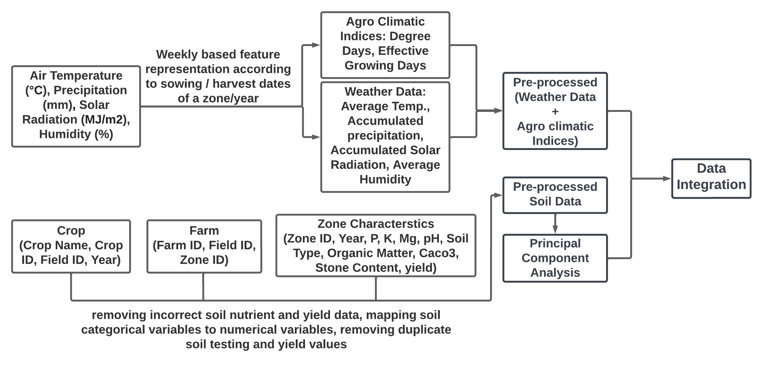
Figure 1: Data pre-processing

The weather variables i.e., air temperature, precipitation, solar radiation, and humidity are represented into weekly based features i.e., each week of all years studied (2013–2018) according to the dynamic sowing and harvest dates of zones/year. After pre-processing of weather data and extracting Two Agro-climatic indices i.e., degree days, and effective growing days are fetched from air temperature weather variables and, used with other weather attributes i.e., average temperature, accumulated precipitation, accumulated solar radiation, and average humidity.

Degree days [12] are calculated as the maximum of 0 and the average of maximum and minimum daily temperature, summed over a week. The total number of days in a week when the average temperature is greater than 5°C is referred to as effective growing days [12]. The average temperature is calculated by averaging the temperature (T) over a week. The accumulated precipitation is calculated by summing precipitation (P) over a week. Solar radiation is summed over a week to get accumulated solar radiation. Humidity (H) is averaged over the week to get average humidity.

After soil and weather data have been pre-processed according to weekly based representation, data integration of weather and soil begins.

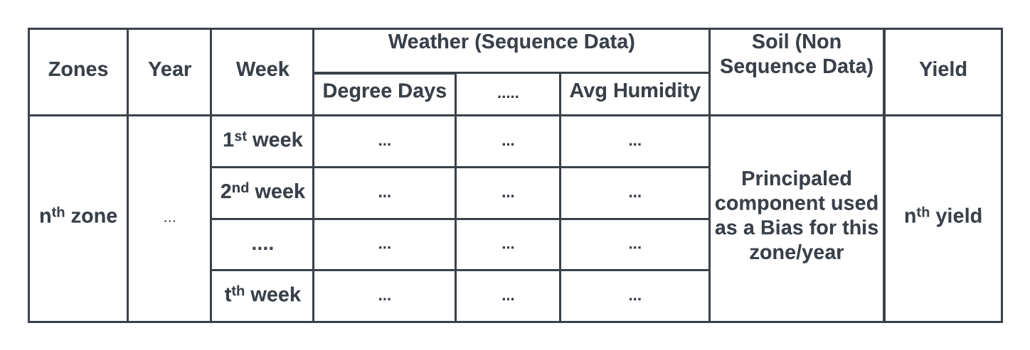
Figure 2: Data pre-processing

Figure 2 illustrates the weekly-based representation i.e., $1^{st}$ week, $2^{nd}$ week, …, $t^{th}$ week of weather data and soil data which is used as a bias for a particular zone and year). This integrated data is further filtered from the growth period of a zone i.e., from $17^{th}$ week till the harvesting period of that zone.

5 Proposed Approach

This study presents a novel approach to handling both sequence and non-sequence data at the same time. We develop a deep learning model to make yield predictions on multiple zones which have different sowing and harvest dates. An epoch is complete when the proposed model in this study is trained on every zone in the dataset exactly once. The applications of classical LSTM are constrained by the requirement that it should have a sequence, i.e., time-series data. However, when we have a mixture of sequence and non-sequence data, a variation is required. Thus, we propose a variant of the classical LSTM that is capable of processing both sequence and non-sequence data. The following proposed approach entails a description of time steps, forward and backward propagation in training, and the steps in testing.

5.1 Training: Description of time steps

Figure 3 shows the time steps in the proposed model. Each time step represents a week i.e., $1\textsuperscript{st}$ time step is $1\textsuperscript{st}$ week; $2\textsuperscript{nd}$ time step is $2\textsuperscript{nd}$ week; and $t\textsuperscript{th}$ time step is $t\textsuperscript{th}$ week. Initially, at the start of $1\textsuperscript{st}$ week, the cell state and hidden state is initialised to 0 which gets updated at each time step based on the input and the previous hidden state. A cell state is the memory of the LSTM which gets updated by the other gates. A hidden state is an output that summarizes the information from the input processed by the LSTM cells.

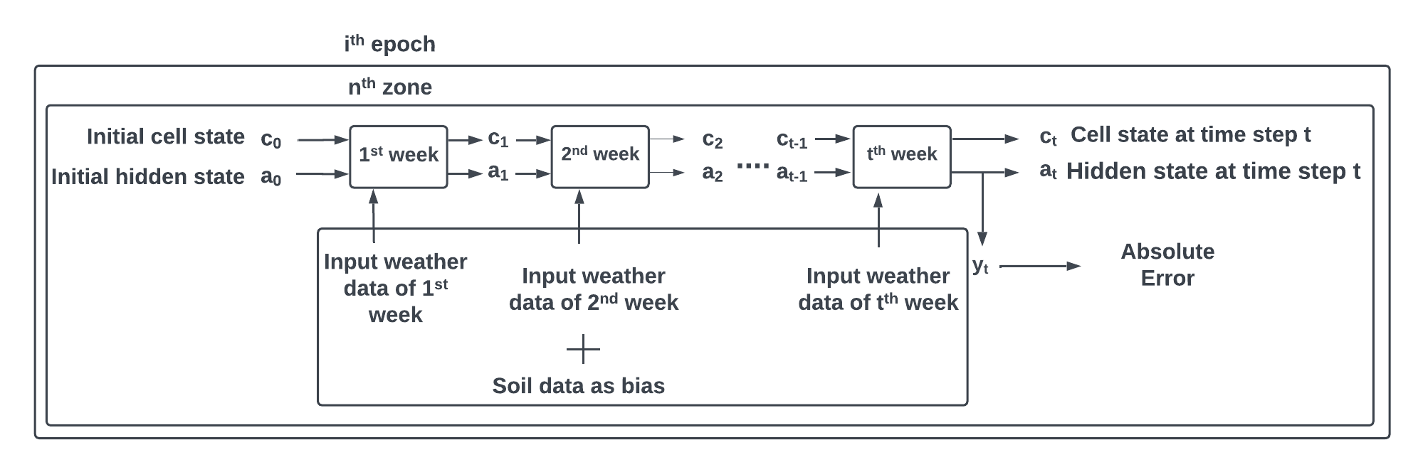
Figure 3: Training Steps (Description of time steps)

Each zone has different weeks because of different sowing and harvesting dates which means the proposed model is trained according to the weeks present in a particular zone. In the forward time step, weather data for each respective week along with bias which is constant over the time steps for a zone is propagated from $1\textsuperscript{st}$ week to $t\textsuperscript{th}$ week of that zone. After $t$ time steps, a yield prediction is computed which is a real number, $y\in\mathbb{R}$. It is then compared with the actual yield to find an absolute error for that zone.

In the backward time step, gradients of weight parameters related to only sequence data i.e., weather data are generated. Here, the parameters are the weights of the network, while the gradients are the derivatives of the loss function with respect to these parameters. Since non-sequence data i.e., the soil remains constant throughout the year for a zone, it is considered as a bias and its gradients are not computed.

5.2 Training: Description of Forward/Backward Propagation

Figure 4 illustrates the forward and backward propagation steps of a proposed deep learning model. It is similar to LSTM architecture except where only gradients of sequence weather data are computed and soil Data is inputted as bias. This figure illustrates one LSTM cell, which corresponds to one zone in one week. Below are the notations used:

• $f_{t}$, $u_{t}$, and $o_{t}$ represents forget, update and output gate respectively. $\int f_{t}$, $\int u_{t}$, and $\int o_{t}$ are the respective derivatives. A forget gate determines which information from the previous cell state should be discarded. An update gate controls how much information from the candidate state should be added to the cell state. An output gate determines which information from the current cell state should be output.

• $w_{fa}$, $w_{ua}$, and $w_{oa}$ are the weight parameters related to the hidden state of forget, update and output gate respectively. $\int w_{fa}$, $\int w_{ua}$, $\int w_{oa}$ are the respective derivatives.

• $w_{fx}$, $w_{ux}$, and $w_{ox}$ are the weight parameters related to weather data of forget, update and output gate respectively. $\int w_{fx}$, $\int w_{ux}$, $\int w_{ox}$ are the respective derivatives.

• $a_{t-1}$, $a_{t}$ represents previous and current hidden state. Similarly, $c_{t-1}$, $c_{t}$ represents previous and current cell state. $\int a_{t-1}$, $\int a_{t}$, $\int c_{t-1}$, $\int c_{t}$ are the respective derivatives.

The description of Forward/Backward Propagation is as follows:-

• In forward propagation, weight parameters of forget gate, update gate, candidate state, output gate and input comprising of weather and soil data are propagated. Here, a candidate state updates the cell state based on the input and the previous hidden state.

• After each time step/week/LSTM cell, cell state and hidden state are updated.

• Calculate the gradients of sequence weather data only by back propagation through time at time step $t$ using the chain rule. No gradients of soil data are computed during back propagation.

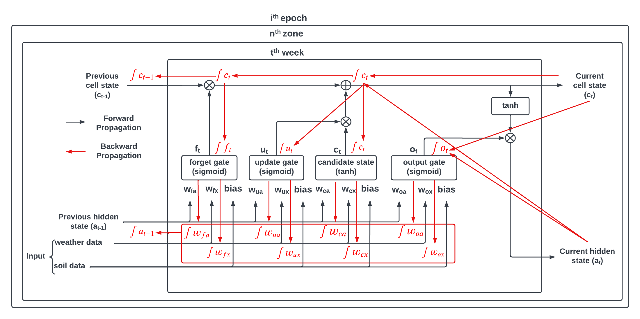
Figure 4: Training (Description of Forward/Backward Propagation)

5.2.1 Training and Testing

Figure 5 shows the training and testing steps of the proposed approach.

The steps in the training stage are as follows:

• Firstly, we set the seed and randomly initialize the weight parameters. The seed is set to ensure that the generated random numbers are reproducible.

• Start the outer loop for the number of epochs the proposed model is trained.

  • For each epoch, there is an inner loop for the number of zones present in the training set. For each zone, do the following:-

    • Do a forward propagation using available parameters from $1\textsuperscript{st}$ week to $t\textsuperscript{th}$ week to generate yield prediction.

    • Compute the absolute error.

    • Do a backward propagation to generate the gradients of weight parameters of different gates. These gradients are the derivatives of the loss function with respect to each of the parameters in the LSTM network.

    • The gradients obtained from the backward propagation are based only on the sequence weather data and are used in the optimisation algorithm to adjust the model parameters during training to minimise the loss function and improve the model’s ability to make accurate predictions on new data. This is where the proposed deep learning model differs from classical LSTM where there was no way to segregate the gradients of heterogeneous data.

    • Absolute errors for all the zones are computed.

  • After the completion of an epoch, mean absolute error is computed and the updated weight parameters are passed from the last zone of the previous epoch to the first zone of the next epoch.

• After the proposed model is trained for all the epochs, we get a training error and the updated weight parameters will be used to evaluate the test set.

The steps in the testing stage are as follows:

• For the test set, the updated weight parameters obtained from the trained model are passed through forward propagation to make a yield prediction.

• Then, absolute error is calculated for a zone.

• After absolute errors for all zones are computed, the mean is taken to find the overall mean absolute error for the test set.

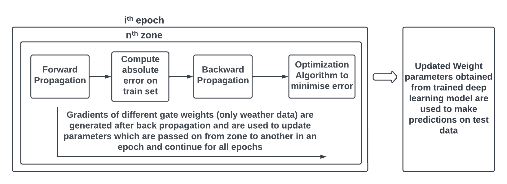
Figure 5: Training and Testing Steps

6 Experiment Setup

The data utilised in this study covers the years 2013 to 2018. We train the proposed deep learning models from 2013 to 2017 and then test it on 2018 dataset. MAE is used as the evaluation metric.

To compare proposed deep learning models with the traditional ML models used in this study [4], we present the weather data in the same two forms: common weather attributes (i.e., temperature, humidity, precipitation, solar radiation), and agro-climatic indices (i.e., degree days, effective growing days). Also, we consider only the growth period weeks beginning from week 17 till the end of the season for modelling.

We have developed 3 deep learning models using the proposed approach which are independent of each other. The first model is using gradient descent [18] optimiser. Second model is using momentum [5] optimiser, and the third model is using Adam [21] optimiser to predict winter wheat yield.

The learning rate is a hyper-parameter that determines the step size while moving towards a minimum of a loss function during the training of a model. During the training process, the goal is to optimize the model parameters to minimize the error between the predicted yield and the actual yield. Hidden units are the intermediate computational units within a neural network that are responsible for processing and transforming the input data into useful representations that can be used to make predictions. Hidden units are the nodes within the neural network that receive input from the previous layer and perform a computation on that input. More hidden units can enable the network to capture more complex patterns in the data, but may also increase the risk of over-fitting, while fewer hidden units may lead to underfitting and poor performance.

To find the best hyper-parameter values for our problem of yield prediction, we performed an exhaustive hyper-parameter search for each model separately using these specific values of hyper-parameters i.e., hidden units from 10, 20, 30, 40; learning rate from 0.001, 0.005, 0.01, 0.05; epochs from 10, 20, 30, 40, 50, 60, 70, 80, 90, 100; Though the optimal hyper-parameter values for an LSTM model depend on the specific task and dataset, however, these are the most commonly used by the authors in the literature who used LSTM on their specific datasets.

For each of these models separately, the proposed approach is applied to the training dataset to get a trained deep learning model and the updated parameters obtained from a trained model are used to make a prediction on the test set.

A comparison is made between the proposed deep learning models and the best-performing ML model i.e., gradient boosting in this study [4]. In addition, the proposed deep learning models are compared among themselves to determine which provides the most accurate yield prediction performance. Statistical significance tests are also done to evaluate if the differences between the MAE values of proposed deep learning models and gradient boosting are significant or not.

7 Experimental Results

This section presents the results for three proposed deep learning models. a) Proposed Deep Learning Model using Gradient Descent optimiser with best hyper-parameters, b) Proposed Deep Learning Model using Momentum optimiser with best hyper-parameters c) Proposed Deep Learning Model using Adam optimiser with best hyper-parameters.

Table 1 shows the MAE of yield prediction in t/h by three proposed models developed in this study and the best performing traditional ML model i.e., Gradient Boosting from the baseline study [4]. Alongside, it also shows the statistical significance tests to measure whether the proposed models improve yield prediction over baseline, our alternative hypothesis is that the MAE of the proposed models is less than the MAE of gradient boosting in the baseline study. Here, p-values are calculated using a one-tailed paired t-test by comparing the absolute errors from a) proposed deep learning models and b) gradient boosting.

Table 1: Winter wheat yield predictions comparison of proposed deep learning model and best ML model from baseline study [4]. Best Hyper-parameters ($h$=Hidden units, $lr$=Learning rate, $e$=Epochs).

Gradient Boosting Model (MAE) - Baseline [4]	Proposed Deep Learning Model (MAE)
	Gradient Descent	Momentum	Adam
	$h$=20,	$h$=10,	$h$=10,
	$lr$=0.01	$lr$=0.005	$lr$=0.005
	$e$=40	$e$=40	$e$=20
1.48	1.31	1.36	1.22
p value	3.2e-5	5.5e-6	9e-4

It is noted that each of the proposed deep learning models surpasses the yield prediction performance of Gradient Boosting. The best set of hyper-parameter values in the first proposed model using gradient descent optimiser is found to be $h$=20, $lr$=40, $e$=0.01. It gives an MAE of 1.31 t/h whereas gradient boosting gives an MAE of 1.48 t/h.

For the second proposed model using momentum optimiser, best hyper-parameters are found to be $h$=10, $lr$=40, $e$=0.005 and it gives an MAE of 1.36 t/h whereas gradient boosting gives an MAE of 1.48 t/h.

The third proposed model using Adam optimiser gives the least MAE of all proposed models with 1.22 t/h with its best hyper-parameters as $h$=10, $lr$=20, $e$=0.005 whereas gradient boosting gives an MAE of 1.48 t/h.

It is noted from the statistical significance tests that p-values for all the proposed models are below the $5\%$ threshold, and thus the alternative hypothesis can be accepted. Consequently, it can be said that yield prediction performances of proposed deep learning models are better than traditional ML models i.e., gradient boosting in the baseline study [4].

8 Conclusion

The purpose of the proposed deep learning models is to predict winter wheat crop yield and determine whether it performs better than the best performing ML model (i.e., Gradient Boosting in the baseline study [4]). We showed that the proposed hybrid approach is able to make better yield predictions than Gradient Boosting. Among the three proposed deep learning models, the hybrid LSTM-Adam model returned the least MAE of 1.22 t/h on the test set, while the gradient Boosting model returned an MAE of 1.48 t/h. As future work, further improvement can be done to these proposed models by adding more feature-engineered agro-climatic indices and by adding more data using spatial interpolation techniques which will be the focus of our next study.

References

- [1] Narayanan Balakrishnan and Govindarajan Muthukumarasamy. Crop production-ensemble machine learning model for prediction. International Journal of Computer Science and Software Engineering, 5(7):148, 2016.
- [2] Nishu Bali and Anshu Singla. Deep learning based wheat crop yield prediction model in punjab region of north india. Applied Artificial Intelligence, 35(15):1304–1328, 2021.
- [3] Nishu Bali and Anshu Singla. Emerging trends in machine learning to predict crop yield and study its influential factors: a survey. Archives of computational methods in engineering, 29(1):95–112, 2022.
- [4] Yogesh Bansal, David Lillis, and Tahar Kechadi. Winter Wheat Crop Yield Prediction on Multiple Heterogeneous Datasets using Machine Learning. In 2022 International Conference on Computational Science and Computational Intelligence (CSCI’22), December 2022.
- [5] Usharani Bhimavarapu, Gopi Battineni, and Nalini Chintalapudi. Improved optimization algorithm in lstm to predict crop yield. Computers, 12(1):10, 2023.
- [6] Nabila Chergui and Mohand Tahar Kechadi. Data analytics for crop management: a big data view. Journal of Big Data, 9(1):1–37, 2022.
- [7] Jichong Han, Zhao Zhang, Juan Cao, Yuchuan Luo, Liangliang Zhang, Ziyue Li, and Jing Zhang. Prediction of winter wheat yield based on multi-source data and machine learning in china. Remote Sensing, 12(2):236, 2020.
- [8] Bing Quan Huang, CJ Du, YB Zhang, and M Tahar Kechadi. A hybrid hmm-svm method for online handwriting symbol recognition. In Intelligent Systems Design and Applications, International Conference on, volume 3, pages 887–891. IEEE Computer Society, 2006.
- [9] S Iniyan, V Akhil Varma, and Ch Teja Naidu. Crop yield prediction using machine learning techniques. Advances in Engineering Software, 175:103326, 2023.
- [10] Jig Han Jeong, Jonathan P Resop, Nathaniel D Mueller, David H Fleisher, Kyungdahm Yun, Ethan E Butler, Dennis J Timlin, Kyo-Moon Shim, James S Gerber, Vangimalla R Reddy, et al. Random forests for global and regional crop yield predictions. PloS one, 11(6):e0156571, 2016.
- [11] Hao Jiang, Hao Hu, Renhai Zhong, Jinfan Xu, Jialu Xu, Jingfeng Huang, Shaowen Wang, Yibin Ying, and Tao Lin. A deep learning approach to conflating heterogeneous geospatial data for corn yield estimation: A case study of the us corn belt at the county level. Global change biology, 26(3):1754–1766, 2020.
- [12] Jordane A Mathieu and Filipe Aires. Assessment of the agro-climatic indices to improve crop yield forecasting. Agricultural and forest meteorology, 253:15–30, 2018.
- [13] Quoc Hung Ngo, Tahar Kechadi, and Nhien-An Le-Khac. Knowledge representation in digital agriculture: A step towards standardised model. Computers and Electronics in Agriculture, 199:107127, 2022.
- [14] Quoc Hung Ngo, Nhien-An Le-Khac, and Tahar Kechadi. Predicting soil ph by using nearest fields. In International Conference on Innovative Techniques and Applications of Artificial Intelligence, pages 480–486. Springer, 2019.
- [15] Vuong M Ngo and M-Tahar Kechadi. Electronic farming records–a framework for normalising agronomic knowledge discovery. Computers and Electronics in Agriculture, 184:106074, 2021.
- [16] Aruvansh Nigam, Saksham Garg, Archit Agrawal, and Parul Agrawal. Crop yield prediction using machine learning algorithms. In 2019 Fifth International Conference on Image Information Processing (ICIIP), pages 125–130. IEEE, 2019.
- [17] Alexandros Oikonomidis, Cagatay Catal, and Ayalew Kassahun. Deep learning for crop yield prediction: a systematic literature review. New Zealand Journal of Crop and Horticultural Science, pages 1–26, 2022.
- [18] Raí A Schwalbert, Telmo Amado, Geomar Corassa, Luan Pierre Pott, PV Vara Prasad, and Ignacio A Ciampitti. Satellite-based soybean yield forecast: Integrating machine learning and weather data for improving crop yield prediction in southern brazil. Agricultural and Forest Meteorology, 284:107886, 2020.
- [19] Sagarika Sharma, Sujit Rai, and Narayanan C Krishnan. Wheat crop yield prediction using deep lstm model. arXiv preprint arXiv:2011.01498, 2020.
- [20] Yulin Shen, Benoît Mercatoris, Zhen Cao, Paul Kwan, Leifeng Guo, Hongxun Yao, and Qian Cheng. Improving wheat yield prediction accuracy using lstm-rf framework based on uav thermal infrared and multispectral imagery. Agriculture, 12(6):892, 2022.
- [21] Jie Sun, Liping Di, Ziheng Sun, Yonglin Shen, and Zulong Lai. County-level soybean yield prediction using deep cnn-lstm model. Sensors, 19(20):4363, 2019.
- [22] Thomas Van Klompenburg, Ayalew Kassahun, and Cagatay Catal. Crop yield prediction using machine learning: A systematic literature review. Computers and Electronics in Agriculture, 177:105709, 2020.
- [23] Xinlei Wang, Jianxi Huang, Quanlong Feng, and Dongqin Yin. Winter wheat yield prediction at county level and uncertainty analysis in main wheat-producing regions of china with deep learning approaches. Remote Sensing, 12(11):1744, 2020.
- [24] Bo Wu, Chongcheng Chen, Tahar Mohand Kechadi, and Liya Sun. A comparative evaluation of filter-based feature selection methods for hyper-spectral band selection. International Journal of Remote Sensing, 34(22):7974–7990, 2013.
- [25] Zijun Zhang. Improved adam optimizer for deep neural networks. In 2018 IEEE/ACM 26th international symposium on quality of service (IWQoS), pages 1–2. Ieee, 2018.