Efficient Dynamics Modeling in Interactive Environments with Koopman Theory

Abstract

The accurate modeling of dynamics in interactive environments is critical for successful long-range prediction. Such a capability could advance Reinforcement Learning (RL) and Planning algorithms, but achieving it is challenging. Inaccuracies in model estimates can compound, resulting in increased errors over long horizons. We approach this problem from the lens of Koopman theory, where the nonlinear dynamics of the environment can be linearized in a high-dimensional latent space. This allows us to efficiently parallelize the sequential problem of long-range prediction using convolution while accounting for the agent’s action at every time step. Our approach also enables stability analysis and better control over gradients through time. Taken together, these advantages result in significant improvement over the existing approaches, both in the efficiency and the accuracy of modeling dynamics over extended horizons. We also show that this model can be easily incorporated into dynamics modeling for model-based planning and model-free RL and report promising experimental results.

1 Introduction

The ability to predict the outcome of an agent’s action over long horizons is a crucial unresolved challenge in Reinforcement Learning (RL) [1, 2, 3, 4]. This is especially important in model-based RL and planning, where deriving a policy from the learned dynamics models allows one to efficiently accomplish a wide variety of tasks in an environment [5, 6, 7, 8, 9]. In fact, state-of-the-art model-free techniques also rely on dynamics models to learn a better representation for downstream value prediction tasks [30]. Thus, obtaining accurate long-range dynamics models in the presence of input and control is crucial. In this work, we leverage techniques and perspectives from Koopman theory [10, 11, 12] to address this key problem in long-range dynamics modeling of interactive environments. The application of Koopman theory allows us to linearise a nonlinear dynamical system by creating a bijective mapping to linear dynamics in a possibly infinite dimensional space of observables.

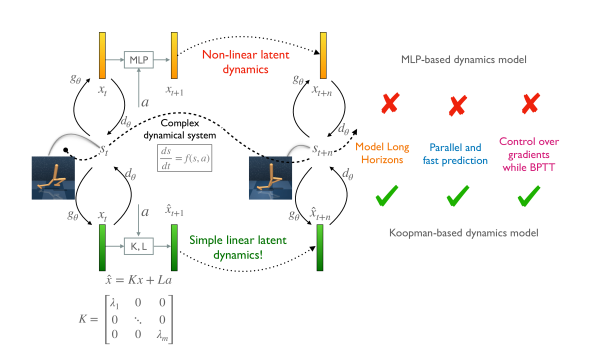
Figure 1: A comparison of our Koopman-based linear dynamics model with a non-linear MLP-based dynamics model. The Diagonal Koopman formulation allows for modeling longer horizons efficiently with control over gradients. Here BPTT stands for Backpropagation Through Time.

Conveniently, a deep neural network can learn to produce such a mapping, enabling a reliable approximation of the non-linear dynamics in the finite dimension of a linear latent space so that only a finite subset of the most relevant (complex-valued) Koopman observables need to be tracked.

We show that this linearization has two major benefits: 1) The eigenvalues of the linear latent-space operator are directly related to the stability and expressive power of the controlled dynamics model. Furthermore, spectral Koopman theory provides a unifying perspective over several existing directions, including long-range sequence modeling using state-space models [13], and the use of unitary matrices [14] in latent dynamic models; 2) This can help to avoid a computational bottleneck due to the sequential nature of dynamics. This is achieved by diagonalization of the linear operator and a reformulation using convolution. In other words, one can perform efficient parallel training of the model over time steps, despite dealing with a controlled dynamical system.

Our experimental results in offline-RL datasets demonstrate the effectiveness of our approach for reward and state prediction over a long horizon. In particular, we report competitive results against dynamics modeling baselines that use Multi-Layer Perceptrons (MLPs), Gated Recurrent Units (GRUs), and Transformers with a similar number of parameters. Finally, we also present encouraging results for model-based planning and model-free RL with our Koopman-based dynamics model.

In summary, our contributions are:

1. The formulation of an efficient linear latent dynamics model from Koopman theory for long-range dynamics modeling in interactive environments.

2. The use of the spectral decomposition of the Koopman matrix showing that this leads to better control over gradients and faster training.

3. The easy integration of our model with existing model-based planning and model-free RL that uses dynamics modeling, leading to enhanced performance and efficiency.

2 Preliminaries

2.1 Koopman Theory for Dynamical Systems

In the context of non-linear dynamical systems, the Koopman operator, a.k.a. the Koopman-von Neumann operator, is a linear operator for studying the system’s dynamics. The Koopman operator is defined as a linear transformation that acts on the space of functions or observables of the system, known as the observables space $\mathcal{F}$. For a non-linear discrete or continuous time dynamical system

$$x_{t+1}=F(x_{t})\quad\text{or}\quad\frac{dx}{dt}=f(x)$$

the Koopman operator $\mathcal{K}:\mathcal{F}\to\mathcal{F}$, is defined as $\mathcal{K}g\cong g\circ F$ where $\mathcal{F}$ is the set of all functions or observables that form an infinite-dimensional Hilbert space. In other words, for every function $g:X\to\mathbb{R}$ belonging to $\mathcal{F}$, where $x_{t}\in X\subset\mathbb{R}^{n}$, we have

$$(\mathcal{K}g)(x_{t})=g(F(x_{t}))=g(x_{t+1}).$$

The infinite dimensionality of the Koopman operator is a limitation in practice, and thus an invariant subspace $\mathcal{G}\subset\mathcal{F}$ is often used, so that $\mathcal{K}g\in\mathcal{G}$. $\mathcal{G}$ is spanned by a finite set of observables ${g_{1},\ldots,g_{m}}$, where often we assume $m\gg n$.

Constraining the Koopman operator on this invariant subspace results in a finite-dimensional linear operator $K\in\mathds{C}^{m\times m}$, called the Koopman matrix, which satisfies $g(x_{t+1})=Kg(x_{t}).$ Usually, the base observation functions $\{g_{i}\}_{i}$ are hand-crafted using knowledge of the system’s underlying physics. However, data-driven methods have recently been proposed to learn the Koopman operator by representing the base observations or their eigenfunction basis using deep neural networks, where a decoder reconstructs the input from linear latent dynamics [e.g.,  15, 16]. Linearizing the dynamics allows for closed-form solutions for the predictions of the dynamical system, as well as stability analysis based on the eigendecomposition of the Koopman matrix.

The observation functions $\{g_{i}\}_{i}$ spanning an invariant subspace can always be chosen to be eigenfunctions $\{{\phi}_{i}\}_{i}$ of the Koopman operator, i.e., $\mathcal{K}\phi_{i}(x)=\lambda_{i}\phi_{i}(x),\forall x$. With this choice of observation functions, the Koopman matrix becomes diagonal,

$$K_{D}=\mathrm{diag}(\lambda_{1},\ldots,\lambda_{m}),\quad\lambda_{i}\in\mathds{C}\quad\forall i.$$ (1)

By using a diagonal Koopman matrix, we are effectively offloading the task of learning the suitable eigenfunctions of the Koopman operator that form an invariant subspace to the neural network encoder. Additionally, for a continuous time input, to be able to model higher-order frequencies in the eigenspectrum and provide better approximations, one could adaptively choose the most relevant eigenvalues and eigenfunctions for the current state [17]. This means $g(x_{t+1})=K_{D}(\lambda(g(x_{t})))g(x_{t}),$ where $\lambda:\mathcal{G}\to\mathds{C}^{m}$ can be a neural network.

2.2 Approximate Koopman with Control Input

The Koopman operator can be extended to non-linear control systems, where the state of the system is influenced by an external control input $u_{t}$ such that $x_{t+1}=F(x_{t},u_{t})$ or $\frac{dx}{dt}=f(x,u)$. Simply treating the pair $(x,u)$ as the input $x$, the Koopman operator becomes $(\mathcal{K}g)(x_{t},u_{t})=g(F(x_{t},u_{t}),u_{t+1})=g(x_{t+1},u_{t+1}).$ For a control affine setting, where

$$f(x,u)=f_{0}(x)+\sum_{i=1}^{m}f_{i}(x)u_{i}$$

one could show that the Koopman operator is bilinearized [12]:

$$g(x_{t+1})=\mathcal{K}(u)g(x_{t})=(\mathcal{K}_{0}+\sum_{i=1}^{m}u_{i}\mathcal{K}_{i})g(x_{t}).$$

More generally, one could make the Koopman operator a function of $u_{t}$, so that the resulting Koopman matrix satisfies $g(x_{t+1})=K(u_{t})g(x_{t})$. This is the approach taken by [18] to model symmetries of dynamics in offline RL. When combined with the diagonal Koopman matrix of Eq. 1, and fixed modulus $|\lambda_{i}|=1\,\forall i$, the Koopman matrix becomes a product of $SO(2)$ representations, and the resulting latent dynamics model, resembles a special setting of the symmetry-based approach of [19], where group representations are used to encode states and state-dependent actions.

An alternate approach to simplifying the Koopman operator with a control signal assumes a decoupling of state and control observables $g(x,u)=[g(x),f(u)]=[g_{1}(x),...,g_{m}(x),f_{1}(u),...,f_{n}(u)]$. This gives rise to a simple linear evolution:

$$g(x_{t+1})=Kg(x_{t})+Lf(u_{t})$$ (2)

where $K\in\mathds{C}^{m\times m}$ and $L\in\mathds{C}^{m\times l}$ are matrices representing the linear dynamics of the state observables and control input, respectively. We build on this approach in our proposed methodology. Although, as shown in [20, 21], even assuming a linear control term $Lu_{t}$ can perform well in practice, we use neural networks for both $f$ and $g$. Our rationale for choosing this formulation is that the additive form of Eq. 2 combined with the diagonalized Koopman matrix of Eq. 1, enable fast parallel training across time-steps using a convolution operation where the convolution kernel can be computed efficiently. Moreover, this setting is amenable to the analysis of gradient behaviour, as discussed in Section 3.2.1.

2.3 Reinforcement Learning

The RL setting can be formalized as a Markov Decision Process (MDP), where an agent learns to make decisions by interacting with an environment. The agent’s goal is to maximize a cumulative reward signal, where a reward function $r(s,a)$ assigns a scalar value to each state-action pair $(s,a)$. The agent’s policy, denoted by $\pi(a|s)$, defines the probability distribution over actions at a given state. The agent’s objective is to learn a policy that maximizes the expected discounted sum of rewards over time, also known as the return: $J(\pi)=\mathbb{E}_{\pi}\left[\sum_{t=0}^{\infty}\gamma^{t}r(s_{t},a_{t})\right]$ where $\gamma\in[0,1]$ is the discount factor and $s_{t}$ and $a_{t}$ are the state and action at time step $t$, respectively. The agent’s expected cumulative reward can also be represented by the Value function, which is defined as the expected cumulative reward starting from a given state and following a given policy.

Value-based RL algorithms have two steps of policy evaluation and policy improvement. For example, $Q$-learning estimates the optimal action-value function, denoted by $Q^{*}(s,a)$, that represents the maximum expected cumulative reward achievable by taking action $a$ in state $s$ and improves the policy by setting it to $arg\max_{a}Q^{*}(s,a)$ [2, 22]. A policy-based RL algorithm directly optimizes the policy to maximize the expected return. Policy gradient methods update the policy by adjusting the policy function’s parameters by estimating the gradient of $J$. Actor-critic methods combine Q-learning and policy gradient ones, such that the Q-network (critic) learns the action value under the current policy, and the policy network (actor) tries to maximize it [23, 24, 25].

2.4 Forward dynamics modeling in RL

Dynamics models have been instrumental in attaining impressive results on various tasks such as Atari [9, 6] and continuous control [6, 26, 27, 28]. By building a model of environment dynamics, model-based RL can generate trajectories used for training the RL algorithm. This can significantly reduce the sample complexity in comparison to model-free techniques. However, in model-based RL, inaccurate long-term predictions can generate poor trajectory rollouts and lead to incorrect expected return calculations, resulting in misleading policy updates. Forward dynamics modeling has also been successfully applied to model-free RL to improve the sample efficiency of the existing model-free algorithms. These methods use it to design self-supervised auxiliary losses for representation learning using consistency in forward dynamics in the latent and the observation space [29, 30, 31].

2.5 Model-based Planning

Model Predictive Control (MPC) is a control strategy that uses a dynamics model $s_{t+1}=f(s_{t},a_{t})$ to plan for a sequence of actions ${a_{t},a_{t+1},\ldots,a_{t+\tau-1}}$ that maximizes the expected return over a finite horizon. The optimization problem is:

$$\arg\max_{a_{t:t+\tau-1}}\mathbb{E}\left[\sum_{i=t}^{t+\tau-1}\gamma^{i}r(s_{i},a_{i})\right]$$ (3)

where $\gamma$ is typically set to 1, that is, there is no discounting. Heuristic population-based methods, such as a cross entropy method [32] are often used for dynamic planning. These methods perform a local trajectory optimization problem, corresponding to the optimization of a cost function up to a certain number of time steps in the future [33, 34, 35]. In contrast to Q-learning, this is myopic and can only plan up to a certain horizon, which is predetermined by the algorithm.

One can also combine MPC with RL to approximate long-term returns of trajectories that can be calculated by bootstrapping the value function of the terminal state. In particular, methods like TD-MPC [8] and LOOP [7] combine value learning with planning using MPC. The learned value function is used to bootstrap the trajectories that are used for planning using MPC. Additionally, they learn a policy using the Deep Deterministic Policy Gradient [36] or Soft Actor-Critic (SAC) [23] to augment the planning algorithm with good proposal trajectories. Alternative search method such as Monte Carlo Tree search [37] is used for planning in discrete action spaces. The performance of the model-based planning method heavily relies on the accuracy of the learned model.

3 Proposed Model

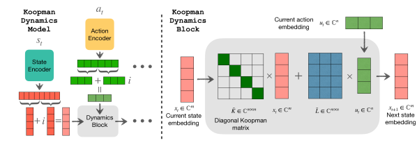
Figure 2: A schematic of the latent Koopman dynamics model. Both actions and initial state embedding are encoded into a latent space in complex ($\mathbb{C}$) domain before passing through the Koopman dynamics block. (see Appendix I for an efficient Jax implementation of the model)

3.1 Linear Latent Dynamics Model

Our task in dynamics modeling is to predict the sequence of future states ${s_{t+1},....,s_{t+\tau}}$ given a starting state $s_{t}$ and some action sequence ${a_{t},a_{t+1},...,a_{t+\tau-1}}$, assuming a Markovian system. Following the second approach described in Section 2.2, we assume that state and control observables are decoupled, and use neural network encoders to encode both states and actions

$$x_{t}=g_{\theta}(s_{t})\quad\text{and}\quad u_{t}=f_{\phi}(a_{t}).$$ (4)

Due to this decoupling, the continuous counterpart of latent space dynamics Eq. 2 is

$$\frac{\mathrm{d}x}{\mathrm{d}t}=Kx(t)+Lu(t),$$ (5)

and the solution is given by $x(s)=e^{Ks}x(0)+\int_{0}^{s}e^{K(s-t)}Lu(t)\mathrm{d}t$ where $e^{Ks}$ is a matrix exponential. One could discretize this to get $\hat{x}_{t+1}=\bar{K}x_{t}+\bar{L}u_{t}$, where $\bar{K}$ and $\bar{L}$ are obtained by Zero-Order Hold (ZOH) discretization of the continuous-time equation [38]:

$$\bar{K}=\exp(\Delta tK)\quad\quad\quad\bar{L}=(K)^{-1}(\exp(\Delta tK)-1)L$$

In practice, we assume that observations are sampled uniformly in time and use a learnable time step parameter $\Delta t$. Unrolling the discrete version of the dynamics for $\tau$ steps, we get:

$$[\hat{x}_{t+1},\cdots,\hat{x}_{t+\tau}]=[\bar{K},\cdots,\bar{K}^{\tau}]x_{t}+[c_{t},\cdots,c_{t+\tau-1}]\underbrace{\begin{bmatrix}I&\bar{K}&\dots&\bar{K}^{\tau-1}\\ 0&I&\cdots&\bar{K}^{\tau-2}\\ \vdots&\vdots&\ddots&\vdots\\ 0&0&\cdots&I\end{bmatrix}}_{\Gamma},$$ (6)

where $c_{t+k}=\bar{L}u_{t+k}$, $\Gamma$ encodes the effect of each input on all future observables, and the $\hat{}$ in $\hat{x}$ distinguishes the prediction from the ground truth observable $x$. (see Appendix B)

We can then recover the predicted state sequence by inverting the function $g_{\theta}$, using a decoder network $\hat{s}_{t+k}=d_{\xi}(\hat{x}_{t+k})$. Loss functions in both input and latent space can be used to learn the encoder, decoder, and latent dynamics model. We refer to these loss functions as the Koopman consistency loss and the state-prediction loss, respectively:

$$\mathcal{L}_{\text{consistency}}=\sum_{k=1}^{\tau}\|\hat{x}_{t+k}-x_{t+k}\|^{2}_{2}\quad\quad\mathcal{L}_{\text{state-pred}}=\sum_{k=1}^{\tau}\|d_{\xi}(\hat{x}_{t+k})-s_{t+k}\|^{2}_{2}$$ (7)

3.2 Diagonalization, Efficiency and Stability of the Koopman Operator

Since the set of diagonalizable matrices is dense in $\mathds{C}^{m\times m}$ and has a full measure, we can always diagonalize the Koopman matrix as shown in Eq. 1. Next, we show that this diagonalization can be leveraged for efficient and parallel forward evolution and training.

To unroll the latent space using Eq. 6 we need to perform matrix exponentiation and dense multiplication. Using a diagonal Koopman matrix $\bar{K}=\mathrm{diag}(\bar{\lambda}_{1},\ldots,\bar{\lambda}_{m})$, this calculation is reduced to computing an $m\times(\tau+1)$ complex-valued Vandermonde matrix:

$$\Lambda=\begin{bmatrix}1&\bar{\lambda}_{1}&\bar{\lambda}_{1}^{2}&\dots&\bar{\lambda}_{1}^{\tau}\\ 1&\bar{\lambda}_{2}&\bar{\lambda}_{2}^{2}&\dots&\bar{\lambda}_{2}^{\tau}\\ \vdots&\vdots&\vdots&\ddots&\vdots\\ 1&\bar{\lambda}_{m}&\bar{\lambda}_{m}^{2}&\dots&\bar{\lambda}_{m}^{\tau}\end{bmatrix}$$ (8)

and doing a row-wise circular convolution of this matrix with a sequence of vectors.

Recall that $x,c\in\mathds{C}^{m}$ are complex vectors. We use superscript to index their elements – i.e., $x_{t}=[x_{t}^{1},\ldots,x_{t}^{m}]$. With this notation, the $i$-th element of the predicted Koopman observables for future time steps is given by (see Appendix B for the derivation):

$$[\hat{x}_{t+1}^{i},\ldots,\hat{x}_{t+\tau}^{i}]=[\bar{\lambda}_{i},\ldots,\bar{\lambda}_{i}^{\tau}]x_{t}^{i}+[1,\bar{\lambda}_{i},\ldots,\bar{\lambda}_{i}^{\tau-1}]\circledast[c_{t}^{i},...,c_{t+\tau-1}^{i}]$$ (9)

where $\circledast$ is circular convolution with zero padding. The convolution can be efficiently computed for longer time steps using Fast Fourier Transform. [39] (see Appendix I)

3.2.1 Gradients Through Time

We show how we can control the behavior of gradients through time by constraining the real part of the eigenvalues of the Diagonal Koopman matrix. Let $\mu$ and $\omega$ refer to the real and imaginary part of the Koopman eigenvalues – that is $\bar{\lambda}_{j}=\mu_{j}+i\omega_{j}$.

Theorem 3.1.

For every time step $k\in\{1,..,\tau\}$ in the discrete dynamics, the norm of the gradient of any loss at $k$-step given by $\mathcal{L}_{k}$ with respect to latent representation at time step $t$ given by $x_{t}$ is a scaled version of the norm of the gradient of the same loss by $x_{t+k}$, where the scaling factor depends on the exponential of the real part of the Koopman eigenvalues, that is:

$$|\frac{\partial\mathcal{L}_{k}}{\partial x_{t}^{j}}|=e^{k\Delta t\mu_{j}}|\frac{\partial\mathcal{L}_{k}}{\partial x_{t+k}^{j}}|\quad\forall j\in\{1,..,m\}.$$

and similarly, for all $l\leq k$, the norm of the gradient of $\mathcal{L}_{k}$ with respect to the control input at time step $t+l-1$ given by is $c_{t+l-1}^{j}$ is a scaled version of the norm of the gradient of $\mathcal{L}_{k}$ by $x_{t+k}$, where the scaling factor depends on the exponential of the real part of the Koopman eigenvalues, that is:

$$|\frac{\partial\mathcal{L}_{k}}{\partial c_{t+l-1}^{j}}|=e^{(k-l)\Delta t\mu_{j}}|\frac{\partial\mathcal{L}_{k}}{\partial\hat{x}_{t+k}^{j}}|\quad\forall j\in\{1,..,m\}$$

A proof of this theorem is provided in Appendix A. The theorem implies that the amplitude of the gradients from a future time step scales exponentially with the real part of each diagonal Koopman eigenvalue. We use this theorem for better initialization of the diagonal Koopman matrix as explained in the next section.

3.2.2 Initialization of the Eigenspectrum

The imaginary part of the eigenvalues of the diagonal Koopman matrix captures different frequency modes of the dynamics. Therefore, it is helpful to initialize them using increasing order of frequency, that is, $\omega_{j}:=\alpha j\pi$, for some constant $\alpha$, to cover a wide frequency range.

From Theorem A.1, we know that the real part of the eigenvalues impacts the gradient’s behavior through time. To avoid vanishing gradients and account for prediction errors over longer horizons, one could eliminate the real part $\mu_{j}:=0$. This choice turns the latent transformations into blocks of 2D rotations [40]. This is also related to using Unitary Matrices to avoid vanishing or exploding gradients in Recurrent Neural Networks [14]. However, intuitively, we might prefer to prioritize closer time steps. This can be done using small negative values e.g., $\mu_{j}\in\{-0.1,-0.2,-0.3\}$. An alternative to having a fixed real part is to turn it into a bounded learnable parameter $\mu_{j}\in[-0.3,-0.1]$. We empirically found $\mu_{j}:=-0.2\;\forall j$, and $\omega_{j}:=j\pi$ to be good choices and use this as our default initialization. In Appendix G we report the results of an ablation study with different initialization schemes.

4 Experiments

While Koopman theory primarily focuses on state prediction, in reinforcement learning (RL) and planning tasks, the model needs to predict various other quantities as well, including rewards, value functions, and policies. These predictions are obtained by adding MLP heads on top of the latent representations. Hence, we give the dynamics model additional flexibility to learn useful representations. This is achieved by relaxing the consistency constraint of Eq. 7 using a loss coefficient that controls its contribution.

Section 4.1 presents our main empirical evaluation on long-range state and reward prediction, in interactive dynamics modeling tasks. Next, Section 4.2 presents the results of experiments on model-free RL and planning.

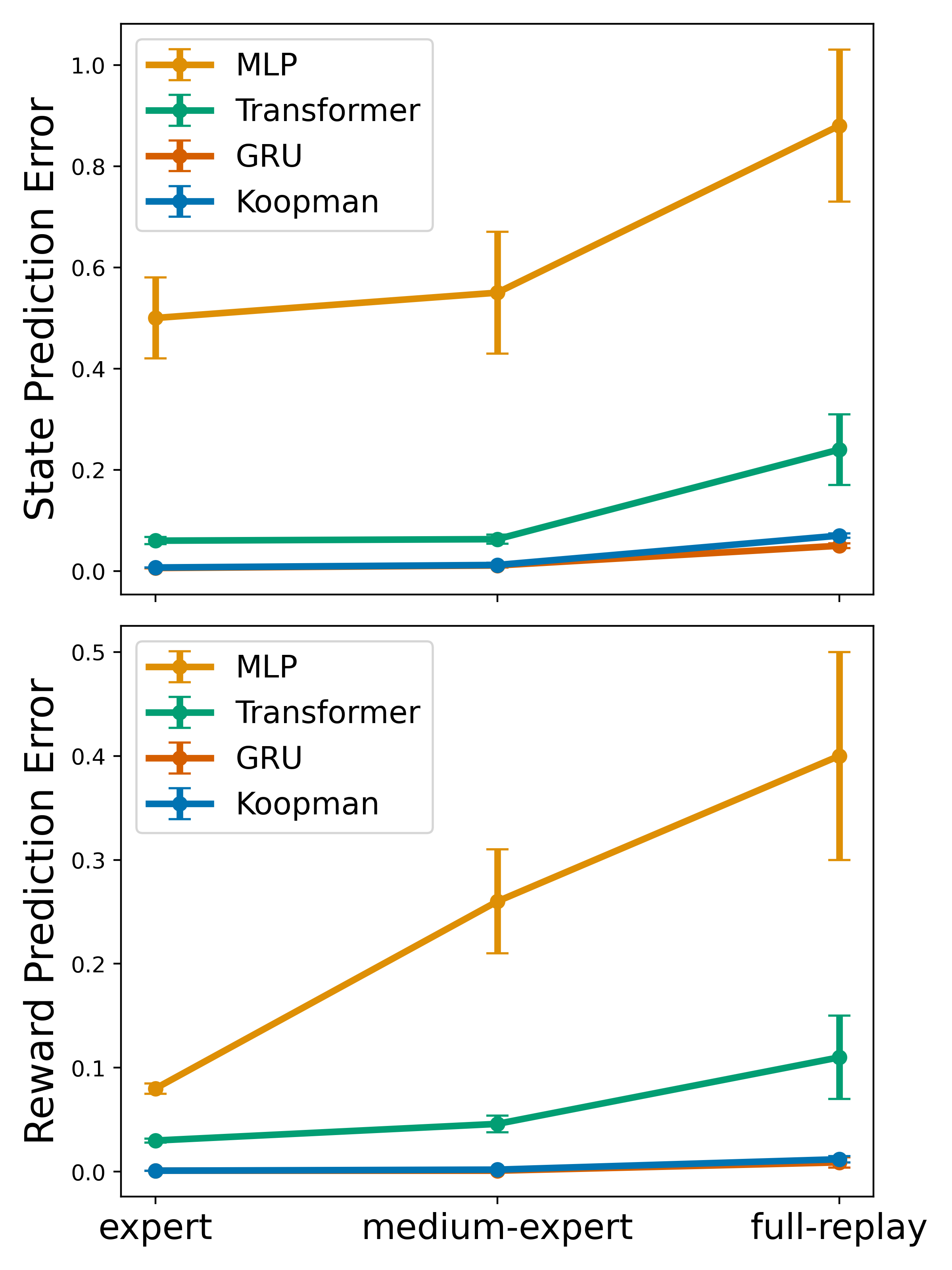
(a) hopper-v2

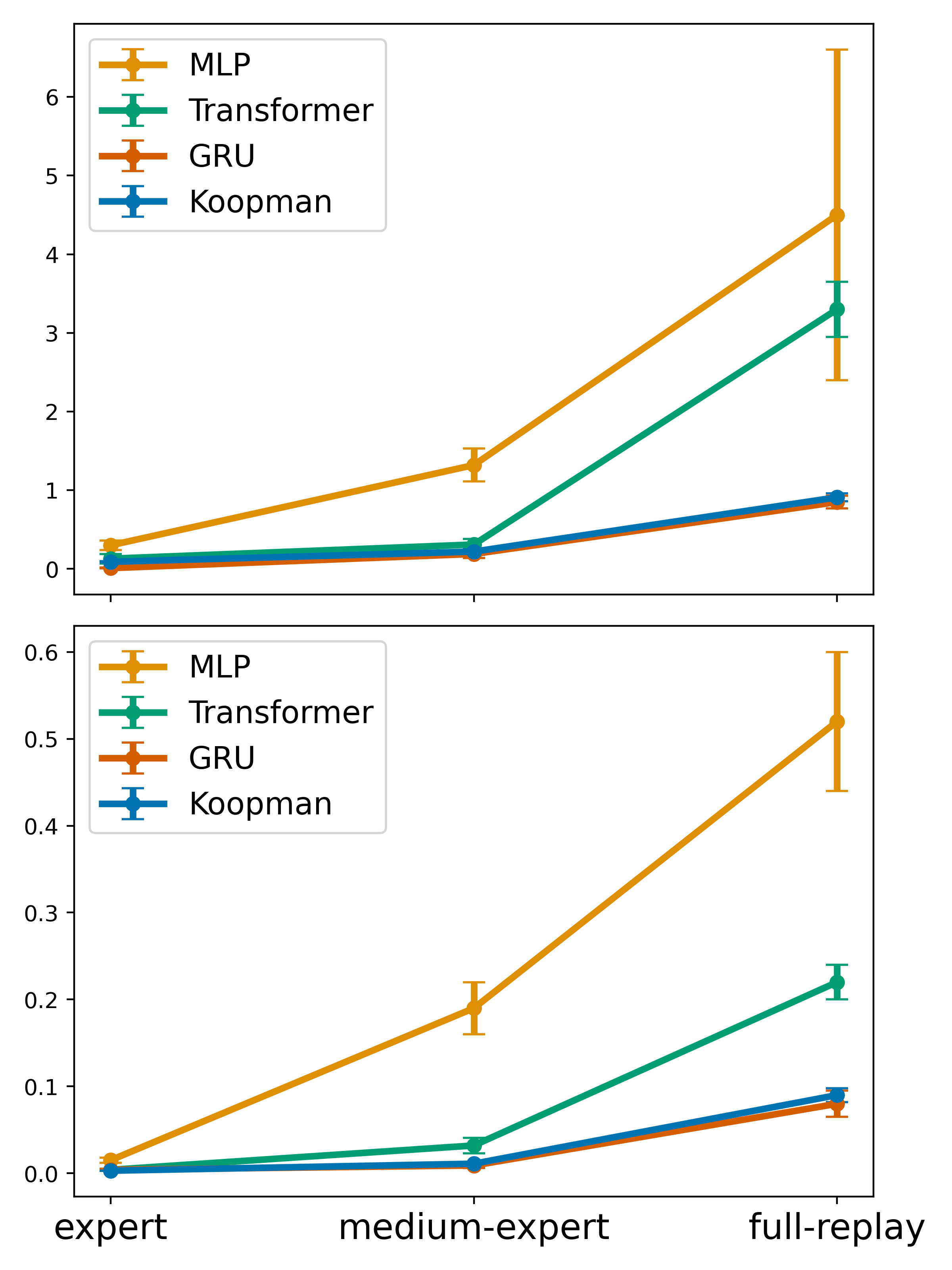
(b) walker2d-v2

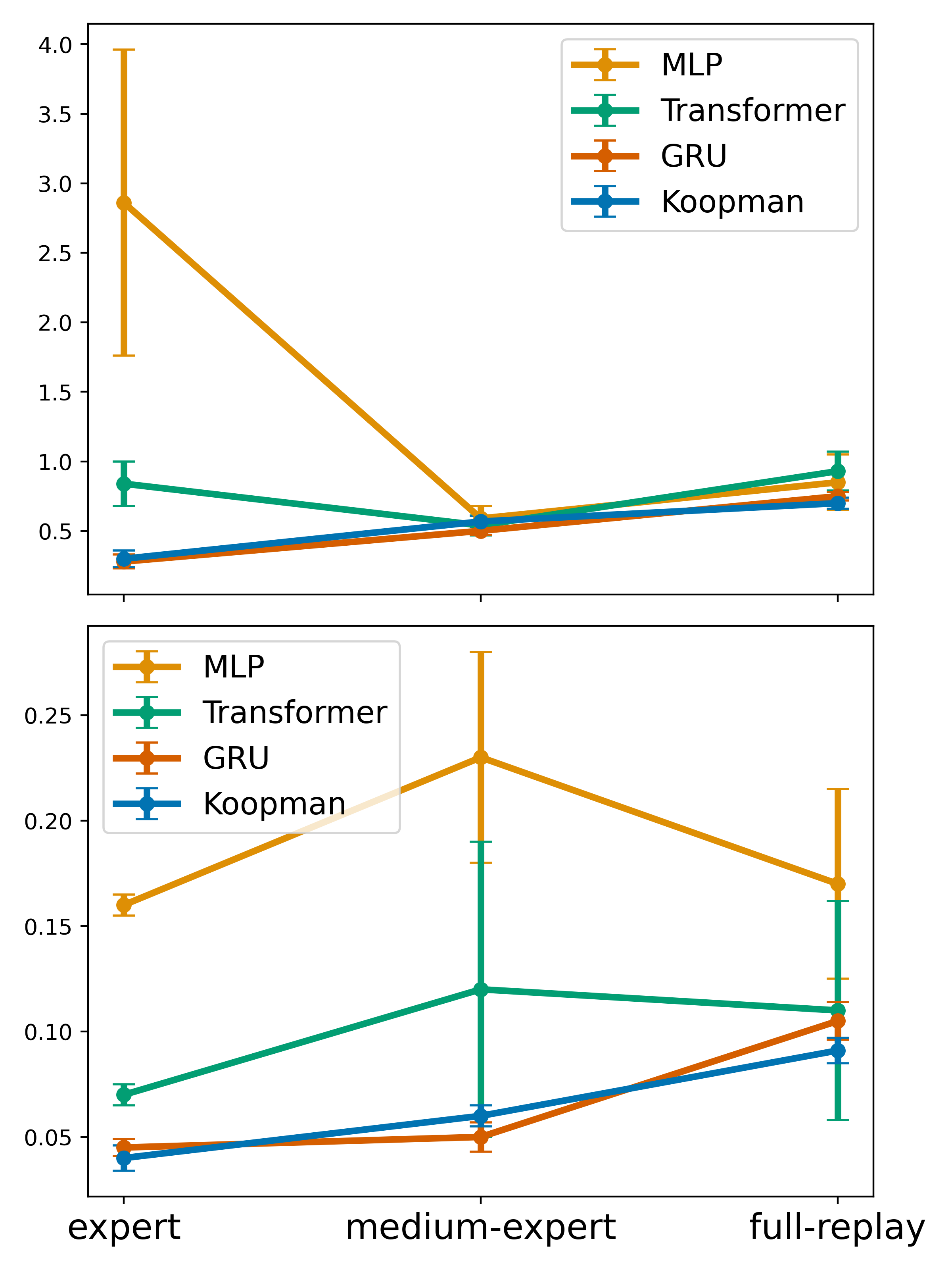
(c) halfcheetah-v2

Figure 3: Forward state and reward prediction error in Offline Reinforcement Learning environments. We consider four dynamics modeling techniques and perform this prediction task over a horizon of 100 environment steps. The results are over 3 runs. See Appendix E for exact numerical values.

4.1 Long-Range Forward Dynamics Modeling with Control

We model the non-linear controlled dynamics of MuJoCo environments [41] using our Koopman operator. We choose a standard MLP-based latent non-linear dynamics model with two linear layers followed by a $\mathrm{ReLU}$ non-linearity as one of our baselines. To make it easier to compare with Koopman dynamics model, we use state embeddings of the same dimensionality using $g_{\theta}$, as described in Section 3.1. This embedding is then fed to the MLP-based latent dynamics model or the diagonal Koopman operator. This approach is widely used in RL for dynamics modeling [7, 8, 9, 30]. To further compare our model with more expressive alternatives that can be trained in parallel, we design a causal Transformer [42, 43] based dynamics model, which takes a masked sequence of state-actions and outputs representations that are used to predict next states and rewards. Finally, following the success of [6], we also design a GRU-based dynamics model that also takes a masked sequence of state-actions to output representations for state and reward prediction. To ensure a fair comparison in terms of accuracy and runtime, we maintain an equal number of trainable parameters for all the aforementioned models. (see Appendix F for more details)

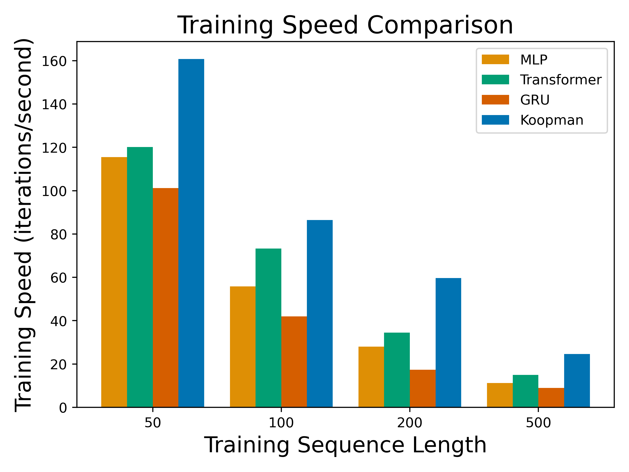
Figure 4: Training speed in iterations/second ($\uparrow$) for a state prediction task using an MLP, a Transformer, a GRU, and our Koopman-based dynamics model on halfcheetah-expert-v2. Each iteration consists of one gradient update of the entire model using a mini-batch of size 256 in one A100 GPU. See Appendix E for exact numerical values.

For the forward dynamics modeling experiments, we use the D4RL [44] dataset, which is a popular offline-RL environment. We select offline datasets of trajectories collected from three different popular Gym-MuJoCo control tasks: hopper, walker, and halfcheetah. These trajectories are obtained from three distinct quality levels of policies, offering a range of data representing various levels of expertise in the task: expert, medium-expert, and full replay. We divide the dataset of 1M samples into 80:20 splits for training and testing, respectively. To train the dynamics model, we randomly sample trajectories of length $\tau$ from the training data, where $\tau$ is the horizon specified during training. We test our learned dynamics model for a horizon length of 100 by randomly sampling 50,000 trajectories of length 100 from the test set. We use our learned dynamics model to predict the ground truth state sequence given the starting state and a sequence of actions.

Training stability

We can only train the MLP-based dynamics model for 10-time steps across all environments. Using longer sequences often results in exploding gradients and instability in training due to backpropagation through time [45]. The alternative of using ${\tanh}$ in MLP-based models can lead to vanishing gradients. In contrast, our diagonal Koopman operator handles long trajectories without encountering vanishing or exploding gradients, in agreement with our discussion in Section 3.2.1.

4.1.1 State and Reward Prediction

In Fig. 3, we evaluate our model’s accuracy in state and reward prediction over long horizons involving 100 environment steps. For this experiment, we add a reward predictor and jointly minimize the reward prediction loss and the state prediction loss. We set the weight of the consistency loss in the latent space to $0.001$. We see that for longer horizon prediction, our model is significantly better in predicting rewards and states accurately for hopper, walker, and halfcheetah in comparison to MLP and Transformer based model while being competitive with GRU-based model. Furthermore, Fig. 4 empirically verifies that our proposed Koopman dynamics model is around twice as fast as an MLP, GRU or Transformer based dynamics model in learning from longer trajectories. The results also reveal the trend that our model’s relative speed-up over baselines grows with the length of the horizon.

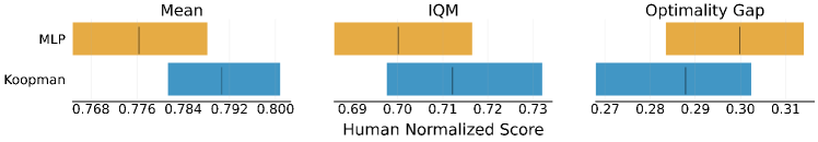
Figure 5: Comparison of our Koopman-based dynamics model (with a horizon of 20) and an MLP-based dynamics model of vanilla TD-MPC [8]. The results are over 5 random seeds for each environment and are presented using the evaluation protocol from [46].

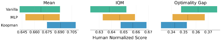
Figure 6: Comparison of vanilla SAC [23] and its integration with an MLP-based (SPR) and a Koopman-based dynamics model for incorporating self-predictive representations in the DeepMind Control Suite. The results are over 5 random seeds for each environment and are presented using the evaluation protocol from [46].

4.2 Koopman Dynamics Model for RL and Planning

We now present promising results in integrating the diagonal Koopman model into (I) model-based planning, and (II) model-free RL, where in the latter, the dynamics model is used for improved representation learning. While the same dynamics model can also be used for (III) model-based RL, we leave that direction for future work.

Evaluation Metric

To assess the performance of our algorithm, we calculate the average episodic return at the conclusion of training and normalize it with the maximum score, i.e., 1000. However, due to significant variance over different runs, relying solely on mean values may not provide reliable metrics. To address this, [46] suggests using bootstrapped confidence intervals (CI) with stratified sampling, which is particularly suitable for small sample sizes, such as the five runs per environment in our case. By utilizing bootstrapped CI, we obtain interval estimates indicating the range within which an algorithm’s aggregate performance is believed to fall and report the Interquartile Mean (IQM). The IQM represents the mean across the middle $50\%$ of the runs, providing a robust measure of central tendency. Furthermore, we calculate the Optimality Gap (OG), which quantifies the extent to which the algorithm falls short of achieving a normalized score of 1.0.

4.2.1 Model-Based Planning

We utilize TD-MPC [8] as the baseline for our model-based planning approach. TD-MPC combines the benefit of a model-free approach in long horizons by learning a value function while using an MLP-based “Task-Oriented Latent Dynamics” (TOLD) model for planning over shorter horizons. To assess the effectiveness of our proposed dynamics model, we replace TOLD with our diagonal Koopman operator. Subsequently, we trained the TD-MPC agent from scratch using this modified Koopman TD-MPC approach. See Section C.1 for details on this adaptation. To evaluate the performance of our variation, we conducted experiments in four distinct environments: Quadruped Run, Quadruped Walk, Cheetah Run, and Acrobot Swingup. We run experiments in the state space and compare them against vanilla TD-MPC.

Our Koopman dynamics model was trained with a horizon of 20-time steps. We observe that TD-MPC suffers from training instability, performance degradation and high variance when using 20-time steps. Consequently, we opted to use a horizon of 5-time steps for the vanilla approach. Fig. 5 suggests that the Koopman TD-MPC outperforms the MLP-based baseline while being more stable.

4.2.2 Model-Free RL

Next, we apply our dynamics model in model-free RL, where we use an adaptation of Self-Predictive Representations [SPR; 30] as our baseline. This adaptation uses an MLP-based dynamics model rather than the original CNN used in SPR in order to eliminate the advantage of the original SPR for image inputs. SPR uses an auxiliary consistency loss similar to Eq. 7, as well as augmentations and other techniques from [47] to prevent representation collapse. It also improves the encoder’s representation quality by making it invariant to the transformations that are not relevant to the dynamics using augmentation; see also [31, 48]. To avoid overconstraining the latent space using the dynamics model, SPR uses projection heads. Similarly, we encode the Koopman observables using a projection layer above the representations used for Q-learning. We provide more details on the integration of the Koopman dynamics model into the SPR framework in Section C.2. The dynamics model is trained to predict representations up to $5$-time steps.

We perform experiments on five different environments from the DeepMind Control (DMC) Suite [49, 50] (Ball in Cup Catch, Cartpole Swingup, Cheetah Run, Finger Spin, and Walker Walk) in pixel space and compare it with an MLP-based dynamics model (SPR) and no dynamics model, i.e., SAC [51] as baselines. Figure 6 demonstrates that Koopman-based model outperforms the SAC plus MLP-based dynamics model baseline while being more efficient.

5 Related Work

Diagonal state space models (DSSMs). DSSMs [13, 53, 54] have been shown to be an efficient alternative to Transformers for long-range sequence modeling. DSSMs with certain initializations have been shown [13] to approximate convolution kernels derived for long-range memory using the HiPPO [55] theory. This explains why DSSMs can perform as well as structured state space models (S4) [56], as pointed out by [53]. Inspired by the success of gating in transformers [57], [54] introduced a gating mechanism in DSS to increase its efficiency further. However, a DSSM is a non-linear model used for sequence modeling and functions differently from our Koopman-based dynamics model, as explained in the comparison with DSSM section in Appendix D.

Probabilistic latent spaces. Several early papers use approximate inference with linear and non-linear latent dynamics so as to provide probabilistic state representations [58, 59, 60, 57, 61]. A common theme in several of these articles is the use of Kalman filtering, using variational inference or MCMC, for estimating the posterior over the latents and mechanisms for disentangled latent representations. While these methods vary in their complexity, scalability, and representation power, similar to an LSTM or a GRU, they employ recurrence and, therefore, cannot be parallelized.

6 Conclusion

Dynamics modeling has a key role to play in sequential decision-making: at training time, having access to a model can lead to sample-efficient training, and at deployment, the model can be used for planning. Koopman theory is an attractive foundation for building such a dynamics model in Reinforcement Learning. The present article shows that models derived from this theoretical foundation can be made computationally efficient. We also demonstrate how this view gives insight into the stability of learning through gradient descent in these models. Empirically, we show the remarkable effectiveness of such an approach in long-range dynamics modeling and provide some preliminary yet promising results for model-based planning and model-free RL.

7 Limitations and Future Work

Although our proposed Koopman-based dynamics model has produced promising results, our current treatment has certain limitations that motivate further investigation. Our current model is tailored for deterministic environments or tasks, overlooking stochastic dynamics modeling. We intend to expand our research in this direction, based on developments around stochastic Koopman theory [52], where Koopman observables become random variables, enabling uncertainty estimation in dynamics. Secondly, although our state prediction task yielded impressive results, we have identified areas for further growth, particularly in enhancing the applications of RL and planning.

We hypothesize that the distribution shift during training and the objective change in training and evaluation hurt the performance of our Koopman dynamics model. We also plan to conduct a more comprehensive study involving a wider range of tasks and environments. Additionally, we aim to explore the compatibility of our model with different reinforcement learning algorithms to showcase its adaptability. Finally, we believe that the diagonal Koopman operator holds promise for model-based RL, where robust dynamics modeling over long horizons is precisely what is currently missing. We intend to investigate this direction, potentially unlocking new avenues for advancement.

Appendix A Proof of Theorem 3.1

Theorem A.1.

For every time step $k\in\{1,..,\tau\}$ in the discrete dynamics, the norm of the gradient of any loss at $k$-step given by $\mathcal{L}_{k}$ with respect to latent representation at time step $t$ given by $x_{t}$ is a scaled version of the norm of the gradient of the same loss by $x_{t+k}$, where the scaling factor depends on the exponential of the real part of the Koopman eigenvalues, that is:

$$|\frac{\partial\mathcal{L}_{k}}{\partial x_{t}^{j}}|=e^{k\Delta t\mu_{j}}|\frac{\partial\mathcal{L}_{k}}{\partial x_{t+k}^{j}}|\quad\forall j\in\{1,..,m\}.$$

and similarly, for all $l\leq k$, the norm of the gradient of $\mathcal{L}_{k}$ with respect to the control input at time step $t+l-1$ given by is $c_{t+l-1}^{j}$ is a scaled version of the norm of the gradient of $\mathcal{L}_{k}$ by $x_{t+k}$, where the scaling factor depends on the exponential of the real part of the Koopman eigenvalues, that is:

$$|\frac{\partial\mathcal{L}_{k}}{\partial c_{t+l-1}^{j}}|=e^{(k-l)\Delta t\mu_{j}}|\frac{\partial\mathcal{L}_{k}}{\partial\hat{x}_{t+k}^{j}}|\quad\forall j\in\{1,..,m\}$$

Proof.

We now provide a proof sketch of Theorem 3.1. As ${\lambda}_{j}=\mu_{j}+i\omega_{j}$, discretizing the diagonal matrix (using ZOH) and taking its $k$-th power gives us $\bar{K}_{j}^{k}=e^{k\Delta t\mu_{j}}e^{ik\Delta t\omega_{j}}$. Using this we can write

$$\hat{x}^{j}_{t+k}=\bar{K}_{j}^{k}x_{t}^{j}+\sum_{l=1}^{k}\bar{K}_{j}^{k-l}c_{t+l-1}^{j}$$

Now applying the chain rule, we get derivatives of the loss with respect to $x_{t}^{j}$ and $c_{t+l-1}^{j}$:

$$\implies\frac{\partial\mathcal{L}_{k}}{\partial x_{t}^{j}}=\frac{\partial\hat{x}_{t+k}^{j}}{\partial x_{t}^{j}}\frac{\partial\mathcal{L}_{k}}{\partial\hat{x}_{t+k}^{j}}=\bar{K}_{j}^{k}\frac{\partial\mathcal{L}_{k}}{\partial\hat{x}_{t+k}^{j}}=e^{k\Delta t\mu_{j}}e^{ik\Delta t\omega_{j}}\frac{\partial\mathcal{L}_{k}}{\partial\hat{x}_{t+k}^{j}}$$

$$\implies\frac{\partial\mathcal{L}_{k}}{\partial c_{t+l-1}^{j}}=\frac{\partial\hat{x}_{t+k}^{j}}{\partial c_{t+l-1}^{j}}\frac{\partial\mathcal{L}_{k}}{\partial\hat{x}_{t+k}^{j}}=\bar{K}_{j}^{k-l}\frac{\partial\mathcal{L}_{k}}{\partial\hat{x}_{t+k}^{j}}=e^{(k-l)\Delta t\mu_{j}}e^{i(k-l)\Delta t\omega_{j}}\frac{\partial\mathcal{L}_{k}}{\partial\hat{x}_{t+k}^{j}}$$

As $|e^{i\theta}|=1$, we get the result of partial derivatives given in Theorem 3.1. ∎

Appendix B Additional Details on the Derivations

We first provide additional steps for the derivation of Eq. 6. As $\hat{x}_{t+1}=\bar{K}x_{t}+\bar{L}u_{t}$, we can unroll it to get future predictions up to $\tau$ time steps that is:

$$\hat{x}_{t+1}=\bar{K}x_{t}+\bar{L}u_{t}$$

$$\hat{x}_{t+2}=\bar{K}\hat{x}_{t+1}+\bar{L}u_{t+1}=\bar{K}(\bar{K}x_{t}+\bar{L}u_{t})+\bar{L}u_{t+1}=\bar{K}^{2}x_{t}+\bar{K}\bar{L}u_{t}+\bar{L}u_{t+1}$$

$$\hat{x}_{t+3}=\bar{K}\hat{x}_{t+2}+\bar{L}u_{t+2}=\bar{K}(\bar{K}^{2}x_{t}+\bar{K}\bar{L}u_{t}+\bar{L}u_{t+1})+\bar{L}u_{t+2}=\bar{K}^{3}x_{t}+\bar{K}^{2}\bar{L}u_{t}+\bar{K}\bar{L}u_{t+1}+\bar{L}u_{t+2}$$

$$\cdots$$

$$\hat{x}_{t+\tau}=\bar{K}^{\tau}x_{t}+\bar{K}^{\tau-1}\bar{L}u_{t}+\bar{K}^{\tau-2}\bar{L}u_{t+1}+\cdots+\bar{L}u_{t+\tau-1}$$

Writing the above equations in a matrix form and using $c_{t+k}=\bar{L}u_{t+k}$ we get Eq. 6. Now to derive Eq. 9, we use the property of matrix exponential of diagonal matrices. In particular, we have $\bar{K}=\mathrm{diag}(\bar{\lambda}_{1},\ldots,\bar{\lambda}_{m})$ implies that $\bar{K}^{\tau}=\mathrm{diag}(\bar{\lambda}_{1}^{\tau},\ldots,\bar{\lambda}_{m}^{\tau})$. Using the notations from Section 3.2, we get that for $i$-th index of predicted vectors $\hat{x}_{t+k}$ s the following equations hold:

$$\hat{x}_{t+1}^{i}=\bar{\lambda_{i}}x_{t}^{i}+c_{t}^{i}$$

$$\hat{x}_{t+2}^{i}=\bar{\lambda_{i}}^{2}x_{t}^{i}+\bar{\lambda_{i}}c_{t}^{i}+c_{t+1}^{i}$$

$$\cdots$$

$$\hat{x}_{t+\tau}^{i}=\bar{\lambda}_{i}^{\tau}x_{t}^{i}+\bar{\lambda}_{i}^{\tau-1}c_{t}^{i}+\bar{\lambda}_{i}^{\tau-2}c_{t+1}^{i}+\cdots+c_{t+\tau-1}^{i}$$

The above equations can be denoted by an expression using the circular convolution operator as written in Eq. 9.

Appendix C Proposed modified dynamics model in RL and Planning

C.1 Koopman TDMPC

TDMPC uses an MLP to design a Task-oriented Latent Dynamica (TOLD) model, which learns to predict the latent representations of the future time steps. The learnt model can then be used for planning. To stabilize training TOLD, the weights of a target encoder network $g_{{\theta}^{-}}$, are updated with the exponential moving average of the online network $g_{\theta}$.

Since dynamics modeling is no longer the only objective, in addition to the latent consistency of Eq. 7, the latent $x^{t}$ is also used to predict the reward and $Q$-function, which takes the latent representations as input. Hence, the dynamics model learns to jointly minimize the following:

$$\mathcal{L}_{\text{TOLD}}=c_{1}\sum_{k=1}^{\tau}\lambda^{k}\| \hat{x}_{t+k}-g_{\theta^{-}}(s_{t+k})\|^{2}_{2}+c_{2}\sum_{k=0}^{\tau}\lambda^{k}\|R_{\theta}(\hat{x}_{t+k},a_{t+k})-r_{t+k}\|^{2}_{2}$$

$$+c_{3}\sum_{k=0}^{\tau}\lambda^{k}\|Q_{\theta}(\hat{x}_{t+k},a_{t+k})-y_{t+k}\|^{2}_{2}$$ (10)

where $R_{\theta}$, $\pi_{\theta}$, $Q_{\theta}$ are respectively reward, policy and Q prediction networks, where $y_{t+k}=r_{t+k}+Q_{\theta^{-}}(\hat{x}_{t+k+1},\pi_{\theta}(\hat{x}_{t+k}))$ is the 1-step bootstrapped TD target. Moreover, the policy network is learned from the latent representation by maximizing the Q value at each time step. This additional policy network helps to provide the next action for the TD target and a heuristic for planning. For details on the planning algorithm and its implementation, see [8].

C.2 Koopman Self-Predictive Representations

To avoid overconstraining the latent space using the dynamics model, SPR uses projection heads. Similarly, we encode the Koopman observables using a projection layer above the representations used for Q-learning. Using $s_{t}$ for the input pixel space, the representation space for the Q-learning is given by $z_{t}=e_{\theta}(s_{t})$ where $e_{\theta}$ is a CNN. The Koopman observables $x_{t}$ is produced by encoding $z_{t}$ using a projector $p_{\theta}$ such that $x_{t}=p_{\theta}(z_{t})$. Moreover, it can be decoded into $z_{t}$ using the decoder $d_{\theta}(\hat{x}_{t})$. Loss functions are the prediction loss Eq. 7 and TD-error

$$\mathcal{L}_{\text{SSL}}=\sum_{k=1}^{\tau}\|d_{\theta}(\hat{x}_{t+k})-e_{\theta^{-}}(s_{t+k})\|^{2}_{2}+\|Q_{\theta}(z_{t},a_{t})-(r_{t}+Q_{\theta^{-}}(e_{\theta^{-}}(s_{t+1}),a_{t+1}))\|^{2}_{2}.$$ (11)

Here, $a_{t+1}$ is sampled from the policy $\pi$. The policy is learned from the representations using Soft Actor-Critic [SAC; 51]. As opposed to SPR, we do not use moving averages for the target encoder parameters and simply stop gradients through the target encoders and denote it as $e_{\theta^{-}}$. Moreover, we drop the consistency term in the Koopman space in Eq. 11 as we empirically observed adding consistency both in Koopman observable ($x$), and Q-learning space ($z$) promotes collapse and makes training unstable, resulting in a higher variance in the model’s performance.

Appendix D Comparison with DSSM

While our proposed Koopman model may look similar to a DSSM [13, 53, 54], there are four major differences. First, our model is specifically derived for dynamics modeling with control input using Koopman theory and not for sequence or time series modeling. Our motivation is to make the dynamics and gradients through time stable, whereas, for DSSMs, it is to approximate the 1D convolution kernels derived from HiPPO [55] theory. Second, a DSSM gives a way to design a cell that is combined with non-linearity and layered to get a non-linear sequence model. In contrast, our Koopman-based model shows that simple linear latent dynamics can be sufficient to model complex non-linear dynamical systems with control. Third, DSSMs never explicitly calculate the latent states and even ignore the starting state. Our model works in the state space, where the starting state is crucial to backpropagate gradients through the state encoder. Fourth, a DSSM learns structured convolution kernels for 1D to 1D signal mapping so that for higher dimensional input, it has multiple latent dynamics models running under the hood, which are implemented as convolutions. In contrast to this, our model runs a single linear dynamics model for any dimensional input.

Appendix E Detailed results from the main text

In this section, we provide the numerical values in Table 1 and Table 2 of the results used in Fig. 3. Table 3 provides the numerical values for training speed used in Fig. 4. In Fig. 7 and Fig. 8, we further provide the environment-wise returns evaluated after every $5000$ training steps for the planning and RL experiments used in Fig. 5 and Fig. 6.

Table 1: Forward state prediction error in Offline Reinforcement Learning environments. The reported number is the mean square error of the state prediction over a horizon of 100 environment steps. The results include standard deviation over 3 runs.

Offline Datasets	State Prediction Error ($\downarrow$)
	MLP	Transformer	GRU	Koopman
hopper-expert-v2	0.500 $\pm$ 0.080	0.060 $\pm$ 0.007	0.006 $\pm$ 0.001	0.007 $\pm$ 0.000
hopper-medium-expert-v2	0.550 $\pm$ 0.120	0.063 $\pm$ 0.009	0.011 $\pm$ 0.004	0.012 $\pm$ 0.004
hopper-full-replay-v2	0.880 $\pm$ 0.150	0.240 $\pm$ 0.070	0.050 $\pm$ 0.005	0.070 $\pm$ 0.004
walker2d-expert-v2	0.300 $\pm$ 0.060	0.130 $\pm$ 0.060	0.010 $\pm$ 0.005	0.090 $\pm$ 0.008
walker2d-medium-expert-v2	1.320 $\pm$ 0.210	0.310 $\pm$ 0.070	0.190 $\pm$ 0.050	0.220 $\pm$ 0.040
walker2d-full-replay-v2	4.500 $\pm$ 2.100	3.300 $\pm$ 0.350	0.850 $\pm$ 0.080	0.910 $\pm$ 0.050
halfcheetah-expert-v2	2.860 $\pm$ 1.100	0.840 $\pm$ 0.160	0.280 $\pm$ 0.050	0.300 $\pm$ 0.060
halfcheetah-medium-expert-v2	0.590 $\pm$ 0.090	0.540 $\pm$ 0.071	0.501 $\pm$ 0.031	0.568 $\pm$ 0.040
halfcheetah-full-replay-v2	0.850 $\pm$ 0.200	0.930 $\pm$ 0.140	0.750 $\pm$ 0.030	0.700 $\pm$ 0.040

Table 2: Forward reward prediction error in Offline Reinforcement Learning environments. The reported number is the mean square error of the reward prediction over a horizon of 100 environment steps. The results include standard deviation over 3 runs.

Offline Datasets	Reward Prediction Error ($\downarrow$)
	MLP	Transformer	GRU	Koopman
hopper-expert-v2	0.080 $\pm$ 0.005	0.030 $\pm$ 0.002	0.001 $\pm$ 0.000	0.001 $\pm$ 0.000
hopper-medium-expert-v2	0.260 $\pm$ 0.050	0.046 $\pm$ 0.008	0.001 $\pm$ 0.000	0.002 $\pm$ 0.000
hopper-full-replay-v2	0.400 $\pm$ 0.100	0.110 $\pm$ 0.040	0.009 $\pm$ 0.005	0.012 $\pm$ 0.003
walker2d-expert-v2	0.015 $\pm$ 0.003	0.004 $\pm$ 0.001	0.004 $\pm$ 0.001	0.003 $\pm$ 0.000
walker2d-medium-expert-v2	0.190 $\pm$ 0.030	0.032 $\pm$ 0.009	0.009 $\pm$ 0.003	0.011 $\pm$ 0.002
walker2d-full-replay-v2	0.520 $\pm$ 0.080	0.220 $\pm$ 0.020	0.080 $\pm$ 0.015	0.090 $\pm$ 0.008
halfcheetah-expert-v2	0.160 $\pm$ 0.050	0.070 $\pm$ 0.005	0.045 $\pm$ 0.004	0.040 $\pm$ 0.006
halfcheetah-medium-expert-v2	0.230 $\pm$ 0.050	0.120 $\pm$ 0.070	0.050 $\pm$ 0.007	0.060 $\pm$ 0.005
halfcheetah-full-replay-v2	0.170 $\pm$ 0.045	0.110 $\pm$ 0.052	0.105 $\pm$ 0.009	0.091 $\pm$ 0.006

Table 3: Training speed (iterations/second) for a state prediction task using an MLP, a Transformer, and a diagonal-Koopman dynamics model on halfcheetah-expert-v2. Each iteration consists of one gradient update of the entire model.

Dynamics Model Type Training sequence length 10 50 100 200 500 MLP 478.00 115.54 55.85 28.02 11.20 Transformer 418.00 120.20 73.34 34.48 14.92 GRU 420.00 101.20 42.02 17.40 08.91 Koopman 565.43 160.76 86.49 59.65 24.56

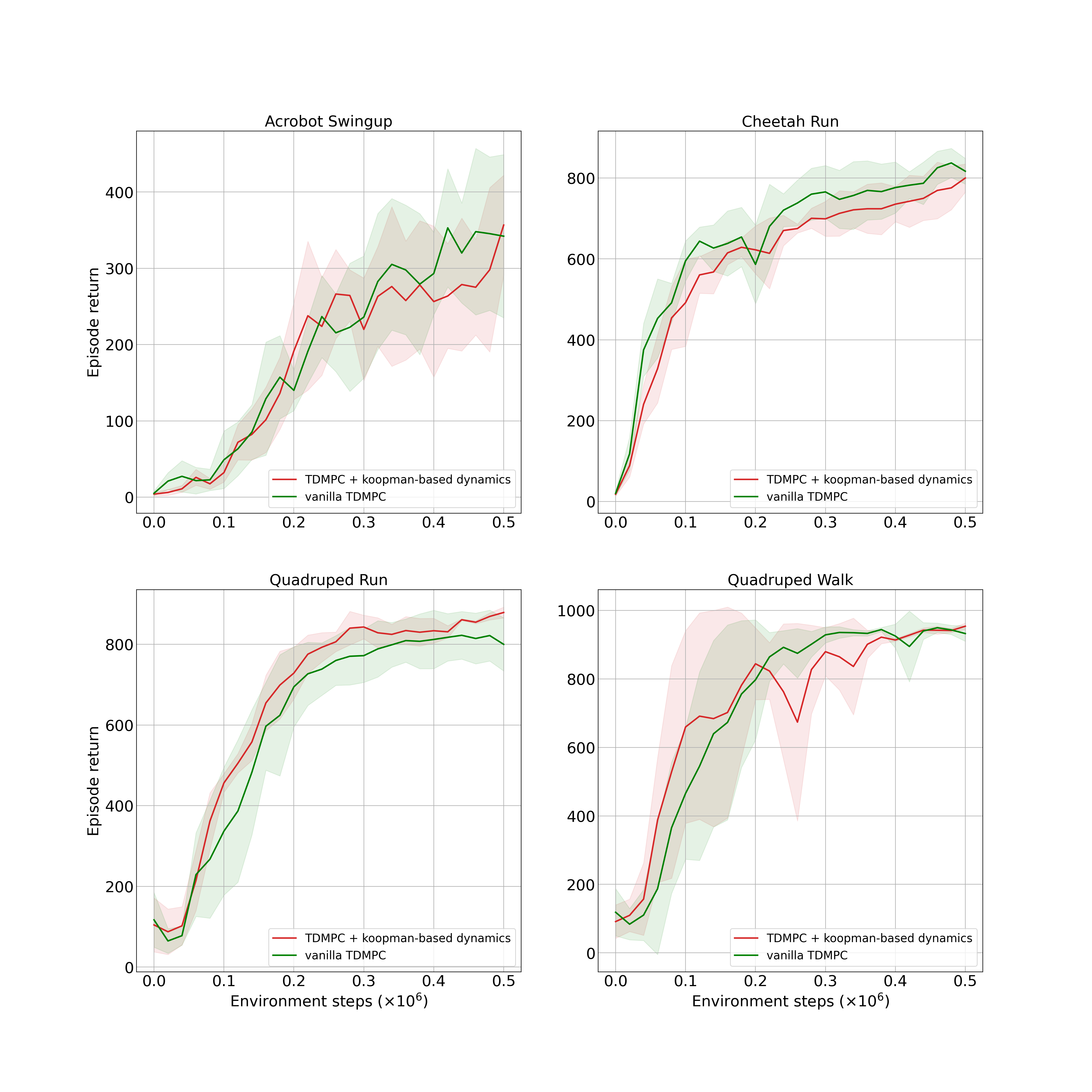
Figure 7: Comparison of our Koopman-based dynamics model (with a horizon of 20) with an MLP-based dynamics model of vanilla TD-MPC [8]. The results are shown with 5 random seeds with the standard deviation shown using the shaded regions.

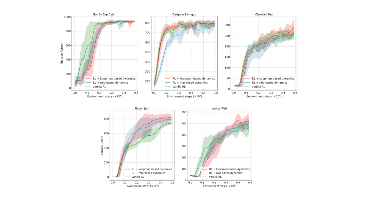
Figure 8: Comparison of vanilla RL (SAC [23]) and its integration with an MLP-based (SPR [30]) and a Koopman-based dynamics model for incorporating self-predictive representations in the DeepMind Control Suite. Shaded regions represent the standard deviation.

Appendix F More details on the baseline dynamics models

For all the experiments, we used a model with around $\sim 500k$ trainable parameters to ensure that the improved compute efficiency during training is not due to the model having fewer parameters. To incorporate the causal transformer architecture with that many parameters, we reduced the embedding dimension of both the state and action embedding to $64$. We further reduced the number of heads to $4$ to design a causal Transformer model that matches the size of our Koopman model. For the GRU and MLP-based model, we keep these dimensions the same as the Koopman one. We use a hidden dimension size of 64 for the GRU based-model in order to keep the parameters similar. Moreover, all our experiments in Table 3 use one Nvidia A100 GPU for training.

Appendix G Ablation study on Initialization

We now perform an ablation study on the different possible initialization methods presented in Section 3.2.2. We report the results for halfcheetah-expert-v2, walker-2d-expert-v2 and hopper-expert-v2, in Table 4, 5 and 6 respectively. We see a constant value of $-0.2$ for $\mu_{i}$, and increasing the order of frequency for $\omega_{i}$ gives a consistent performance boost over different environments.

Table 4: Ablation on initialization of the eigenvalues of the diagonal Koopman matrix: $\lambda_{i}=\mu_{i}+j\omega_{i}$ for halfcheetah-expert-v2. The results are over three seeds.

$\mu_{i}$ $\omega_{i}$ State Prediction Error ($\downarrow$) Reward Prediction Error ($\downarrow$) constant increasing 0.300 $\pm$ 0.060 0.040 $\pm$ 0.006 constant random 0.340 $\pm$ 0.047 0.041 $\pm$ 0.005 learnable increasing 0.320 $\pm$ 0.024 0.048 $\pm$ 0.003 learnable random 0.360 $\pm$ 0.040 0.042 $\pm$ 0.007

Table 5: Ablation on initialization of the eigenvalues of the diagonal Koopman matrix: $\lambda_{i}=\mu_{i}+j\omega_{i}$ for walker-2d-expert-v2. The results are over three seeds.

$\mu_{i}$ $\omega_{i}$ State Prediction Error ($\downarrow$) Reward Prediction Error ($\downarrow$) constant increasing 0.090 $\pm$ 0.008 0.003 $\pm$ 0.000 constant random 0.104 $\pm$ 0.008 0.004 $\pm$ 0.001 learnable increasing 0.102 $\pm$ 0.003 0.004 $\pm$ 0.000 learnable random 0.096 $\pm$ 0.007 0.003 $\pm$ 0.002

Table 6: Ablation on initialization of the eigenvalues of the diagonal koopman matrix: $\lambda_{i}=\mu_{i}+j\omega_{i}$ for hopper-expert-v2. The results are over three seeds.

$\mu_{i}$ $\omega_{i}$ State Prediction Error ($\downarrow$) Reward Prediction Error ($\downarrow$) constant increasing 0.007 $\pm$ 0.000 0.001 $\pm$ 0.000 constant random 0.010 $\pm$ 0.007 0.014 $\pm$ 0.005 learnable increasing 0.008 $\pm$ 0.006 0.002 $\pm$ 0.004 learnable random 0.008 $\pm$ 0.004 0.003 $\pm$ 0.001

Appendix H Ablation on the dimensionality of Linear latent space

We also ablate the dimensionality of the Koopman state observables: $m$ in Table 7 and show that a $512$ is enough for most of the environments, as the performance saturates there.

Table 7: Forward state prediction error in Offline Reinforcement Learning environments. The reported number is the mean square error of the state prediction in halfcheetah-expert-v2 over a horizon of 100 environment steps. We observe a general trend of a decrease in the error values with an increase in the state embedding dimension which is aligned with the Koopman theory. We have selected an embedding dimension of 512 for all our experiments as it has the lowest error value.

State Embedding Dim. ($m$) State Prediction Error ($\downarrow$) 128 0.0097 256 0.0081 512 0.0073 1024 0.0075

Appendix I Koopman dynamics model in jax

We provide the Jax code snippet to efficiently implement our Koopman-based dynamics model.

Algorithm 1 Diagonal Koopman Dynamics model

⬇

import jax

import jax.numpy as jnp

from jax.nn.initializers import normal

from flax import linen as nn

# Main class to implement Diagonal Koopman Dynamics model

class BatchedDiagonalKoopmanDynamicsModel(nn.Module):

state_dim: int

action_emb_dim: int

real_init_type: str = ’constant’

real_init_value: float = -0.5

im_init_type: str = ’increasing_freq’

activations: Callable[[jnp.ndarray], jnp.ndarray] = nn.relu

def init_koopman_imaginary_params(self):

if self.im_init_type == ’increasing_freq’:

self.K_im = self.param(

"K_im", increasing_im_init(), (self.state_dim // 4,)

)

elif self.im_init_type == ’random’:

self.K_im = self.param(

"K_im", random_im_init(), (self.state_dim // 4,)

)

else:

raise ValueError

def init_koopman_real_params(self):

if self.real_init_type == ’constant’:

self.K_real = self.real_init_value

elif self.real_init_type == ’learnable’:

self.K_r = self.param(

"K_real", nn.initializers.ones, (self.state_dim // 4,)

) * self.real_init_value

self.K_real = jnp.clip(self.K_r, -0.4, -0.1)

else:

raise ValueError

def setup(self):

# model parameters

self.init_koopman_real_params()

self.init_koopman_imaginary_params()

self.action_encoder = MLP(

[128, self.action_emb_dim * 2],

activations=self.activations

)

self.L = self.param(

"L", normal(0.1), (self.action_emb_dim, self.state_dim // 2, 2)

)

# Step parameter

self.step = jnp.exp(self.param("log_step", log_step_init(), (1,)))

self.K_complex = jnp.concatenate(

[self.K_real + 1j * self.K_im,

self.K_real - 1j * self.K_im],

axis=-1

)

self.L_complex = self.L[:, :, 0] + 1j * self.L[:, :, 1]

self.K_dis, self.L_dis = discretize(

self.K_complex, self.L_complex, self.step

)

def __call__(self, actions, start_state_rep):

if len(actions.shape) == 2:

return koopman_forward_single(

self.K_dis, self.L_dis,

self.action_encoder(actions), start_state_rep

)

else:

Vand_K = jnp.vander(

self.K_dis, actions.shape[1] + 1, increasing=True

)

return koopman_forward(

Vand_K, self.L_dis,

self.action_encoder(actions), start_state_rep

)

Algorithm 2 Helper functions for Diagonal Koopman Dynamics model

⬇

def causal_convolution(u, K):

assert K.shape[0] == u.shape[0]

ud = jnp.fft.fft(jnp.pad(u, (0, K.shape[0])))

Kd = jnp.fft.fft(jnp.pad(K, (0, u.shape[0])))

out = ud * Kd

return jnp.fft.ifft(out)[: u.shape[0]]

def compute_measurement_block(Ker, action_emb, init_state):

return causal_convolution(action_emb, Ker[:-1]) + Ker[1:] * init_state

def compute_measurement(Ker, action_emb, init_state):

return jax.vmap(

compute_measurement_block,

in_axes=(0, 1, 0),

out_axes=1

)(Ker, action_emb, init_state)

def discretize(K, L, step):

return jnp.exp(step*K), (jnp.exp(step*K)-1)/K * L

def log_step_init(dt_min=0.001, dt_max=0.1):

def init(key, shape):

return jax.random.uniform(key, shape) * (

jnp.log(dt_max) - jnp.log(dt_min)

) + jnp.log(dt_min)

return init

def increasing_im_init():

def init(key, shape):

return jnp.pi * jnp.arange(shape[0])

return init

def random_im_init():

def init(key, shape):

return jax.random.uniform(key, shape)

return init

@jit

def koopman_forward(Vand_K, L, actions_emb, start_state_rep):

action_emb_dim = actions_emb.shape[-1]

state_dim = start_state_rep.shape[-1]

actions_emb_complex = actions_emb[:, :, :action_emb_dim//2] \

+ 1j * actions_emb[:, :, action_emb_dim//2:]

start_state_rep_complex = start_state_rep[:, :state_dim // 2] \

+ 1j * start_state_rep[:, state_dim // 2:]

predicted_state_rep_complex = jax.vmap(

compute_measurement,

in_axes=(None, 0, 0),

out_axes=0

)(Vand_K, actions_emb_complex @ L, start_state_rep_complex)

predicted_state_rep = jnp.concatenate([

jnp.real(predicted_state_rep_complex),

jnp.imag(predicted_state_rep_complex)

], -1)

return predicted_state_rep

@jit

def koopman_forward_single(K, L, action_emb, start_state_rep):

action_emb_dim = action_emb.shape[-1]

state_dim = start_state_rep.shape[-1]

action_emb_complex = action_emb[:, :action_emb_dim//2] \

+ 1j * action_emb[:, action_emb_dim//2:]

start_state_rep_complex = start_state_rep[:, :state_dim // 2] \

+ 1j * start_state_rep[:, state_dim // 2:]

predicted_state_rep_complex = K[None, :] * start_state_rep_complex + \

.action_emb_complex @ L

predicted_state_rep = jnp.concatenate([

jnp.real(predicted_state_rep_complex),

jnp.imag(predicted_state_rep_complex)

], -1)

return predicted_state_rep

References

- [1] Richard S Sutton and Andrew G Barto. Reinforcement learning: An introduction. MIT press, 2018.
- [2] Volodymyr Mnih, Koray Kavukcuoglu, David Silver, Andrei A. Rusu, Joel Veness, Marc G. Bellemare, Alex Graves, Martin Riedmiller, Andreas K. Fidjeland, Georg Ostrovski, Stig Petersen, Charles Beattie, Amir Sadik, Ioannis Antonoglou, Helen King, Dharshan Kumaran, Daan Wierstra, Shane Legg, and Demis Hassabis. Human-level control through deep reinforcement learning. Nature, 518(7540):529–533, 2015.
- [3] David Silver, Aja Huang, Chris J Maddison, Arthur Guez, Laurent Sifre, George Van Den Driessche, Julian Schrittwieser, Ioannis Antonoglou, Veda Panneershelvam, and Marc Lanctot. Mastering the game of go with deep neural networks and tree search. Nature, 550:354–359, 2017.
- [4] Volodymyr Mnih, Adria Puigdomenech Badia, Mehdi Mirza, Alex Graves, Timothy Lillicrap, Tim Harley, David Silver, and Koray Kavukcuoglu. Asynchronous methods for deep reinforcement learning. ICML, 2016.
- [5] Yilun Du and Karthic Narasimhan. Task-agnostic dynamics priors for deep reinforcement learning. In International Conference on Machine Learning, pages 1696–1705. PMLR, 2019.
- [6] Danijar Hafner, Timothy Lillicrap, Jimmy Ba, and Mohammad Norouzi. Dream to control: Learning behaviors by latent imagination. In International Conference on Learning Representations, 2020.
- [7] Harshit Sikchi, Wenxuan Zhou, and David Held. Learning off-policy with online planning. In 5th Annual Conference on Robot Learning, 2021.
- [8] Nicklas A Hansen, Hao Su, and Xiaolong Wang. Temporal difference learning for model predictive control. In Kamalika Chaudhuri, Stefanie Jegelka, Le Song, Csaba Szepesvari, Gang Niu, and Sivan Sabato, editors, Proceedings of the 39th International Conference on Machine Learning, volume 162 of Proceedings of Machine Learning Research, pages 8387–8406. PMLR, 17–23 Jul 2022.
- [9] Julian Schrittwieser, Ioannis Antonoglou, Thomas Hubert, Karen Simonyan, Laurent Sifre, Simon Schmitt, Arthur Guez, Edward Lockhart, Demis Hassabis, Thore Graepel, et al. Mastering atari, go, chess and shogi by planning with a learned model. Nature, 588(7839):604–609, 2020.
- [10] Bernard O Koopman. Hamiltonian systems and transformation in hilbert space. Proceedings of the National Academy of Sciences, 17(5):315–318, 1931.
- [11] Bernard O Koopman and J v Neumann. Dynamical systems of continuous spectra. Proceedings of the National Academy of Sciences, 18(3):255–263, 1932.
- [12] Steven L Brunton, Marko Budišić, Eurika Kaiser, and J Nathan Kutz. Modern koopman theory for dynamical systems. arXiv preprint arXiv:2102.12086, 2021.
- [13] Albert Gu, Karan Goel, Ankit Gupta, and Christopher Ré. On the parameterization and initialization of diagonal state space models. In Alice H. Oh, Alekh Agarwal, Danielle Belgrave, and Kyunghyun Cho, editors, Advances in Neural Information Processing Systems, 2022.
- [14] Martin Arjovsky, Amar Shah, and Yoshua Bengio. Unitary evolution recurrent neural networks. In International conference on machine learning, pages 1120–1128. PMLR, 2016.
- [15] Bethany Lusch, J Nathan Kutz, and Steven L Brunton. Deep learning for universal linear embeddings of nonlinear dynamics. Nature communications, 9(1):1–10, 2018.
- [16] Kathleen Champion, Bethany Lusch, J Nathan Kutz, and Steven L Brunton. Data-driven discovery of coordinates and governing equations. Proceedings of the National Academy of Sciences, 116(45):22445–22451, 2019.
- [17] Bethany Lusch, J. Nathan Kutz, and Steven L. Brunton. Deep learning for universal linear embeddings of nonlinear dynamics. Nature Communications, 9, 2017.
- [18] Matthias Weissenbacher, Samarth Sinha, Animesh Garg, and Kawahara Yoshinobu. Koopman q-learning: Offline reinforcement learning via symmetries of dynamics. In Kamalika Chaudhuri, Stefanie Jegelka, Le Song, Csaba Szepesvari, Gang Niu, and Sivan Sabato, editors, Proceedings of the 39th International Conference on Machine Learning, volume 162 of Proceedings of Machine Learning Research, pages 23645–23667. PMLR, 17–23 Jul 2022.
- [19] Arnab Kumar Mondal, Vineet Jain, Kaleem Siddiqi, and Siamak Ravanbakhsh. EqR: Equivariant representations for data-efficient reinforcement learning. In Kamalika Chaudhuri, Stefanie Jegelka, Le Song, Csaba Szepesvari, Gang Niu, and Sivan Sabato, editors, Proceedings of the 39th International Conference on Machine Learning, volume 162 of Proceedings of Machine Learning Research, pages 15908–15926. PMLR, 17–23 Jul 2022.
- [20] Steven L Brunton, Joshua L Proctor, and J Nathan Kutz. Discovering governing equations from data by sparse identification of nonlinear dynamical systems. Proceedings of the national academy of sciences, 113(15):3932–3937, 2016.
- [21] Daniel Bruder, Brent Gillespie, C David Remy, and Ram Vasudevan. Modeling and control of soft robots using the koopman operator and model predictive control. arXiv preprint arXiv:1902.02827, 2019.
- [22] Volodymyr Mnih, Koray Kavukcuoglu, David Silver, Alex Graves, Ioannis Antonoglou, Daan Wierstra, and Martin A. Riedmiller. Playing atari with deep reinforcement learning. CoRR, 2013.
- [23] Tuomas Haarnoja, Aurick Zhou, Pieter Abbeel, and Sergey Levine. Soft actor-critic: Off-policy maximum entropy deep reinforcement learning with a stochastic actor, 2018.
- [24] Timothy P. Lillicrap, Jonathan J. Hunt, Alexander Pritzel, Nicolas Heess, Tom Erez, Yuval Tassa, David Silver, and Daan Wierstra. Continuous control with deep reinforcement learning. In Yoshua Bengio and Yann LeCun, editors, ICLR, 2016.
- [25] John Schulman, Filip Wolski, Prafulla Dhariwal, Alec Radford, and Oleg Klimov. Proximal policy optimization algorithms. ArXiv, abs/1707.06347, 2017.
- [26] Xiaoyu Jiang, Qiuxuan Chen, Shiyi Han, Mingxuan Li, Jingyan Dong, and Ruochen Zhang. When to trust your model: Model-based policy optimization, 2020. Submitted to NeurIPS 2019 Reproducibility Challenge.
- [27] Harshit Sikchi, Wenxuan Zhou, and David Held. Learning off-policy with online planning. In 5th Annual Conference on Robot Learning, 2021.
- [28] Kendall Lowrey, Aravind Rajeswaran, Sham Kakade, Emanuel Todorov, and Igor Mordatch. Plan online, learn offline: Efficient learning and exploration via model-based control. In International Conference on Learning Representations, 2019.
- [29] Max Jaderberg, Volodymyr Mnih, Wojciech Marian Czarnecki, Tom Schaul, Joel Z Leibo, David Silver, and Koray Kavukcuoglu. Reinforcement learning with unsupervised auxiliary tasks. In International Conference on Learning Representations, 2017.
- [30] Max Schwarzer, Ankesh Anand, Rishab Goel, R. Devon Hjelm, Aaron C. Courville, and Philip Bachman. Data-efficient reinforcement learning with self-predictive representations. In International Conference on Learning Representations, 2020.
- [31] A. Srinivas, Michael Laskin, and P. Abbeel. Curl: Contrastive unsupervised representations for reinforcement learning. In International Conference on Machine Learning, 2020.
- [32] Reuven Y Rubinstein and Dirk P Kroese. The cross-entropy method: a unified approach to combinatorial optimization, Monte-Carlo simulation, and machine learning, volume 133. Springer, 2004.
- [33] Grady Williams, Andrew Aldrich, and Evangelos Theodorou. Model predictive path integral control using covariance variable importance sampling, 2015.
- [34] Grady Williams, Paul Drews, Brian Goldfain, James M Rehg, and Evangelos A Theodorou. Information-theoretic model predictive control: Theory and applications to autonomous driving. IEEE Transactions on Robotics, 34(6):1603–1622, 2018.
- [35] Masashi Okada and Tadahiro Taniguchi. Variational inference mpc for bayesian model-based reinforcement learning. In Leslie Pack Kaelbling, Danica Kragic, and Komei Sugiura, editors, Proceedings of the Conference on Robot Learning, volume 100 of Proceedings of Machine Learning Research, pages 258–272. PMLR, 30 Oct–01 Nov 2020.
- [36] Timothy P. Lillicrap, Jonathan J. Hunt, Alexander Pritzel, Nicolas Manfred Otto Heess, Tom Erez, Yuval Tassa, David Silver, and Daan Wierstra. Continuous control with deep reinforcement learning. CoRR, abs/1509.02971, 2015.
- [37] Rémi Coulom. Efficient selectivity and backup operators in monte-carlo tree search. In International conference on computers and games, pages 72–83. Springer, 2006.
- [38] Arieh Iserles. A first course in the numerical analysis of differential equations. Number 44. Cambridge university press, 2009.
- [39] E Oran Brigham. The fast Fourier transform and its applications. Prentice-Hall, Inc., 1988.
- [40] Arnab Kumar Mondal, Vineet Jain, Kaleem Siddiqi, and Siamak Ravanbakhsh. Eqr: Equivariant representations for data-efficient reinforcement learning. In International Conference on Machine Learning, pages 15908–15926. PMLR, 2022.
- [41] Emanuel Todorov, Tom Erez, and Yuval Tassa. Mujoco: A physics engine for model-based control. In 2012 IEEE/RSJ International Conference on Intelligent Robots and Systems, 2012.
- [42] Ashish Vaswani, Noam Shazeer, Niki Parmar, Jakob Uszkoreit, Llion Jones, Aidan N Gomez, Łukasz Kaiser, and Illia Polosukhin. Attention is all you need. Advances in neural information processing systems, 30, 2017.
- [43] Lili Chen, Kevin Lu, Aravind Rajeswaran, Kimin Lee, Aditya Grover, Misha Laskin, Pieter Abbeel, Aravind Srinivas, and Igor Mordatch. Decision transformer: Reinforcement learning via sequence modeling. Advances in neural information processing systems, 34:15084–15097, 2021.
- [44] Justin Fu, Aviral Kumar, Ofir Nachum, George Tucker, and Sergey Levine. D4rl: Datasets for deep data-driven reinforcement learning, 2020.
- [45] Ilya Sutskever. Training recurrent neural networks. University of Toronto Toronto, ON, Canada, 2013.
- [46] Rishabh Agarwal, Max Schwarzer, Pablo Samuel Castro, Aaron C Courville, and Marc Bellemare. Deep reinforcement learning at the edge of the statistical precipice. Advances in neural information processing systems, 34:29304–29320, 2021.
- [47] Jean-Bastien Grill, Florian Strub, Florent Altché, Corentin Tallec, Pierre Richemond, Elena Buchatskaya, Carl Doersch, Bernardo Avila Pires, Zhaohan Guo, Mohammad Gheshlaghi Azar, et al. Bootstrap your own latent-a new approach to self-supervised learning. Advances in neural information processing systems, 33:21271–21284, 2020.
- [48] Denis Yarats, Ilya Kostrikov, and Rob Fergus. Image augmentation is all you need: Regularizing deep reinforcement learning from pixels. In International Conference on Learning Representations, 2021.
- [49] Saran Tunyasuvunakool, Alistair Muldal, Yotam Doron, Siqi Liu, Steven Bohez, Josh Merel, Tom Erez, Timothy Lillicrap, Nicolas Heess, and Yuval Tassa. dm_control: Software and tasks for continuous control. Software Impacts, 6:100022, 2020.
- [50] Yuval Tassa, Yotam Doron, Alistair Muldal, Tom Erez, Yazhe Li, Diego de Las Casas, David Budden, Abbas Abdolmaleki, Josh Merel, Andrew Lefrancq, et al. Deepmind control suite. arXiv preprint arXiv:1801.00690, 2018.
- [51] Tuomas Haarnoja, Aurick Zhou, Pieter Abbeel, and Sergey Levine. Soft actor-critic: Off-policy maximum entropy deep reinforcement learning with a stochastic actor. In Jennifer Dy and Andreas Krause, editors, Proceedings of the 35th International Conference on Machine Learning, volume 80 of Proceedings of Machine Learning Research, pages 1861–1870. PMLR, 10–15 Jul 2018.
- [52] Igor Mezić. Spectral properties of dynamical systems, model reduction and decompositions. Nonlinear Dynamics, 41:309–325, 2005.
- [53] Ankit Gupta, Albert Gu, and Jonathan Berant. Diagonal state spaces are as effective as structured state spaces. Advances in Neural Information Processing Systems, 35:22982–22994, 2022.
- [54] Harsh Mehta, Ankit Gupta, Ashok Cutkosky, and Behnam Neyshabur. Long range language modeling via gated state spaces. arXiv preprint arXiv:2206.13947, 2022.
- [55] Albert Gu, Tri Dao, Stefano Ermon, Atri Rudra, and Christopher Ré. Hippo: Recurrent memory with optimal polynomial projections. Advances in neural information processing systems, 33:1474–1487, 2020.
- [56] Albert Gu, Karan Goel, and Christopher Re. Efficiently modeling long sequences with structured state spaces. In International Conference on Learning Representations, 2022.
- [57] Weizhe Hua, Zihang Dai, Hanxiao Liu, and Quoc Le. Transformer quality in linear time. In International Conference on Machine Learning, pages 9099–9117. PMLR, 2022.
- [58] Tuomas Haarnoja, Anurag Ajay, Sergey Levine, and Pieter Abbeel. Backprop kf: Learning discriminative deterministic state estimators. Advances in neural information processing systems, 29, 2016.
- [59] Philipp Becker, Harit Pandya, Gregor Gebhardt, Cheng Zhao, C James Taylor, and Gerhard Neumann. Recurrent kalman networks: Factorized inference in high-dimensional deep feature spaces. In International conference on machine learning, pages 544–552. PMLR, 2019.
- [60] Vaisakh Shaj, Philipp Becker, Dieter Büchler, Harit Pandya, Niels van Duijkeren, C James Taylor, Marc Hanheide, and Gerhard Neumann. Action-conditional recurrent kalman networks for forward and inverse dynamics learning. In Conference on Robot Learning, pages 765–781. PMLR, 2021.
- [61] Marco Fraccaro, Simon Kamronn, Ulrich Paquet, and Ole Winther. A disentangled recognition and nonlinear dynamics model for unsupervised learning. Advances in neural information processing systems, 30, 2017.