Fast quantum algorithm for differential equations

Abstract

Partial differential equations (PDEs) are ubiquitous in science and engineering. Prior quantum algorithms for solving the system of linear algebraic equations obtained from discretizing a PDE have a computational complexity that scales at least linearly with the condition number $\kappa$ of the matrices involved in the computation. For many practical applications, $\kappa$ scales polynomially with the size $N$ of the matrices, rendering a polynomial-in-$N$ complexity for these algorithms. Here we present a quantum algorithm with a complexity that is polylogarithmic in $N$ but is independent of $\kappa$ for a large class of PDEs. Our algorithm generates a quantum state that enables extracting features of the solution. Central to our methodology is using a wavelet basis as an auxiliary system of coordinates in which the condition number of associated matrices is independent of $N$ by a simple diagonal preconditioner. We present numerical simulations showing the effect of the wavelet preconditioner for several differential equations. Our work could provide a practical way to boost the performance of quantum-simulation algorithms where standard methods are used for discretization.

Partial differential equations (PDEs) are an integral part of many mathematical models in science and engineering. The common approach to solving a PDE on a digital computer is mapping it into a matrix equation by a discretization method and solving the matrix equation using numerical algorithms. The time complexity of the best-known classical algorithm for solving a linear matrix equation obtained from discretizing a linear PDE scales polynomially with the size $N$ and condition number $\kappa$ of matrices involved in the computation [1, 2, 3]; $\kappa$ is defined as the ratio of the largest to smallest singular values of a matrix. In contrast, several quantum algorithms, known as quantum linear-system algorithms (QLSAs) [3, 4, 5, 6, 7, 8, 9, 10, 11], have been developed for solving a system of linear equations with a complexity that grows at least linearly with $\kappa$, and it cannot be made sublinear in $\kappa$ for a general system of linear equations by standard complexity-theoretic assumptions [3].

A key challenge in solving differential equations is arising ill-conditioned matrices (i.e., matrices with large $\kappa$) after the discretization. The condition number of these matrices generally grows polynomially with their size $N$; it grows as $N^{2}$ for second-order differential equations. Such ill-conditioned matrices not only lead to numerical instabilities for solutions but also eliminate the exponential improvement of existing quantum algorithms with respect to $N$. Despite the extensive previous work on efficient quantum algorithms for differential equations [12, 13, 14, 15, 16, 17, 18, 19, 2], the challenge of ill-conditioned matrices remains as these algorithms require resources that grow with $\kappa$.

In this paper, we establish a quantum algorithm for a large class of inhomogeneous PDEs with a complexity that is polylogarithmic in $N$ and is independent of $\kappa$. Our algorithm’s complexity does not violate the established lower bound on the complexity of solving a linear system [3] as the lower bound is for generic cases. With respect to complexity lower bounds, the class of differential equations we consider is similar to the class of ‘fast-forwardable’ Hamiltonians [20, 21, 22, 23]: Hamiltonians that are simulatable in a sublinear time and do not violate the “no-fast-forwarding” theorem [24]. Therefore, we refer to the class of differential equations solvable in a polylogarithmic time as the class of ‘fast-solvable’ differential equations.

The core of our methodology is utilizing wavelets for preconditioning (i.e., controlling the condition number of) the linear system associated with a PDE. Wavelets are versatile bases with appealing features [25, 26, 27, 28], such as having local basis functions in both position and momentum space, making them advantageous for applications in quantum physics and computation [29, 30, 31, 32, 33, 34], and computational chemistry [35]. A notable feature of wavelets is that they provide an optimal preconditioner for a large class of operators by a simple diagonal preconditioner [36, 37, 38, 39, 40]. The preconditioner is optimal in the sense that the preconditioned matrices have uniformly bounded condition numbers independent of their size; the condition number is constant and only depends on the wavelet type (see FIG. 1). The preconditioner is also a ‘structured’ diagonal matrix with a particular structure on its diagonals; see FIG. 1(b). We exploit the optimality and structure of the wavelet preconditioner to perform matrix manipulations on a quantum computer that leads to a polylogarithmic-time quantum algorithm for solving a discretized version of certain PDEs.

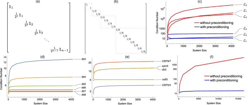
Figure 1: (a) The diagonal wavelet preconditioner with size $2^{n}$; $n=4$ is shown in (b). The matrix has a block-diagonal structure with blocks of exponentially increasing size. Diagonals are constant within each block but are exponentially decreasing from block to block. (c) Condition numbers with and without preconditioning for  $\mathcal{L}_{1}:=\frac{\text{d}^{2}}{\text{d}x^{2}}$, $\mathcal{L}_{2}:=\frac{\text{d}^{2}}{\text{d}x^{2}}-\frac{\text{d}}{\text{d}x}+\mathbbm{1}$ and $\mathcal{L}_{3}:=-\frac{\text{d}}{\text{d}x}\left(\cosh(x/4)\frac{\text{d}}{\text{d}x}\right)+\text{e}^{x}\mathbbm{1}$, all discretized by finite-difference method on a grid with periodic boundaries. Here system size is the number of grid points and the Daubechies wavelet with index 3 is used for preconditioning. (d) The condition number decreases by increasing the wavelet index. (e) The condition number depends on the type of wavelet used but is independent of system size. Only $\mathcal{L}_{1}$ is preconditioned in (d) and (e). Symlet (sym3), Daubechies (db3) and Coiflet (coif3) wavelets [26] with index 3, and Cohen–Daubechies–Feauveau (CDF) wavelets of type “9/7” and “5/3” [41] are used. (f) Condition numbers for 2D Laplacian $\mathcal{L}:=\frac{\text{d}^{2}}{\text{d}x^{2}}+\frac{\text{d}^{2}}{\text{d}y^{2}}$ discretized by finite-difference method on a square grid with periodic boundaries.

We note that the differential equation does not need to be discretized by wavelets. Standard methods such as the finite-difference method could be used for discretization. In this case, we use wavelets only as a tool to perform linear-algebra manipulation of the linear system obtained by the finite-difference method. That is to say that a wavelet basis provides an auxiliary system of coordinates in which the condition numbers of the matrices involved in the computation are under control. Employing such a hybrid approach yields a practical way to significantly boost the performance of algorithms based on standard discretization methods and shows the advantage of performing computations in wavelet bases.

Methodologically, we first transform the system of linear equations obtained by the finite-difference discretization into a wavelet basis. Then we precondition the wavelet-transformed system with the wavelet preconditioner to have a linear system with a uniform condition number. By this preconditioning, a direct approach to obtaining a quantum solution for the original linear system is to generate a quantum state encoding the solution of the preconditioned system by QLSAs, which would have a $\kappa$-independent cost, and then transform the generated state to a quantum state that encodes the solution of the original system. This transformation requires applying the wavelet preconditioner $P$ shown in FIG. 1(a). As $P$ is nonunitary, it needs to be implemented probabilistically. However, because the condition number of $P$ is $\mathcal{O}(N)$, the success probability is small, rendering an $\mathcal{O}(N)$-time algorithm (see Appendix C).

To construct a polylogarithmic algorithm, we avoid directly applying $P$. Instead, we add two ancilla qubits to the $n$-qubit system and generate a quantum state in the space of $n+2$ qubits so that the generated state enables computing the expectation value of some given $n$-qubit observable $M$, a Hermitian operator associated with a physical quantity. As the generated state is in the extended space, we need to construct an $(n+2)$-qubit observable $M^{\prime}$ so that the expectation value of $M^{\prime}$ with respect to the generated state yields the expectation value of $M$ with respect to the $n$-qubit state encoding the solution of the original linear system. The observable $M^{\prime}$ we construct is a 4-by-4 block matrix with $M$ in each block. By this block structure, we construct a specification of $M^{\prime}$ (i.e., oracles specifying $M^{\prime}$) using one query to specification of $M$.

Our approach requires performing two diagonal unitaries with the same structure as the preconditioner and constructing a block-encoding for the inverse of the preconditioned matrix. We use the bounded condition number of the preconditioned matrix, the preconditioner’s structure and properties of a wavelet transformation to perform each of these operations in a polylogarithmic time, yielding a polylogarithmic algorithm for generating a quantum solution for certain PDEs.

Notations.—We use $\left\lVert A\right\rVert$ for the 2-norm (or the operator norm) of an operator $A$, $\left\lVert\bm{v}\right\rVert$ for the 2-norm of a vector $\bm{v}$ and $\left\lVert f\right\rVert$ for the 2-norm of a function $f$. We refer to $A\in\mathbb{C}^{2^{n}\times 2^{n}}$ as $n$-qubit matrix and denote the $n$-qubit identity by $\mathbbm{1}_{n}$. We use the technique of block encoding [6], which is a way of embedding a matrix as a block of a larger unitary matrix. Formally, for $\varepsilon>0$ and a number of qubits $a$, an $(\alpha,a,\varepsilon)$–block-encoding of an $n$-qubit matrix $A$ is an $(n+a)$-qubit unitary $U_{A}$ such that $\left\lVert A-\alpha(\bra{0^{a}}\otimes\mathbbm{1}_{n})U_{A}(\ket{0^{a}}\otimes\mathbbm{1}_{n})\right\rVert\leq\varepsilon$, where $\alpha\geq\left\lVert A\right\rVert$.

Outline.—The rest of this paper proceeds as follows. First, we specify the class of fast-solvable PDEs. Then we detail our approach, present the algorithm and analyze its complexity. We conclude with a discussion of limitations and extensions. Proofs of stated lemmas and detailed complexity analysis are provided in the Appendix.

Fast-solvable PDEs.—We now specify the class of PDEs for which wavelets provide an optimal preconditioner. We begin with some terminology. A $d$-dimensional ($d$D) linear PDE is formally written as $\mathcal{L}u(\bm{x})=b(\bm{x})$, where $\bm{x}$ is an element of a bounded domain $\Omega\subset\mathbb{R}^{d}$, $u(\bm{x})$ and the inhomogeneity $b(\bm{x})$ are scalar functions, and $\mathcal{L}$ is a linear operator acting on $u(\bm{x})$. For a linear PDE of order $m$, $\mathcal{L}$ has the form $\sum_{\bm{\alpha}}c_{\bm{\alpha}}(\bm{x})\partial^{\bm{\alpha}}u$ where $\bm{\alpha}=(\alpha_{1},\ldots,\alpha_{d})$ is a multi-index with non-negative elements such that $|\bm{\alpha}|:=\alpha_{1}+\cdots+\alpha_{d}\leq m$, each coefficient $c_{\bm{\alpha}}(\bm{x})$ is a scalar function, and $\partial^{\bm{\alpha}}u:=\partial^{\alpha_{1}}_{1}\cdots\partial^{\alpha_{d}}_{d}u$ with $\partial^{\alpha_{i}}_{i}$ the partial derivative of order $\alpha_{i}$ with respect to $x_{i}$. For all nonzero $\bm{\xi}^{\bm{\alpha}}:=\xi^{\alpha_{1}}_{1}\cdots\xi^{\alpha_{d}}_{d}$ with $\xi^{\alpha_{i}}_{i}\in\mathbb{R}^{d}$ and all $\bm{x}\in\Omega$, if $\sum_{|\bm{\alpha}|=m}c_{\bm{\alpha}}(\bm{x})\bm{\xi}^{\bm{\alpha}}\neq 0$, then $\mathcal{L}$ is called ‘elliptic’ operator and its corresponding PDE is called elliptic PDE.

Let $B(u,v):=\int u(\bm{x})\mathcal{L}v(\bm{x})\,\text{d}\bm{x}$ be the bilinear form induced by $\mathcal{L}$ on the space $\mathcal{H}$ of sufficiently differentiable functions; $B$ is a bilinear map $\mathcal{H}\times\mathcal{H}\mapsto\mathbb{R}$. The class of differential operators for which the bilinear form $B(u,v)$ is

1. symmetric: $B(u,v)=B(v,u)$,

2. bounded: $B(u,v)\leq C\left\lVert u\right\rVert\left\lVert v\right\rVert$, and

3. coercive (or elliptic): $B(u,u)\geq c\left\lVert u\right\rVert^{2}$, for $0<c<C$,

comprises the PDEs that are optimally preconditionable by wavelets [36, 37, 38]; the Lax–Milgram theorem asserts existence and uniqueness of solution for the variational form of these PDEs [42]. This class includes prevalent differential equations such as Poisson, Helmholtz, biharmonic and time-independent Schrödinger equations. A particular subclass is the second-order PDEs called Sturm-Liouville problems [39, 43] with an operator of form $\mathcal{L}u(\bm{x})=-\sum_{ij=1}^{d}\partial_{j}(p_{ij}(\bm{x})\partial_{i}u)+q(\bm{x})u$, where $0\leq q(\bm{x})\leq C_{q}$ and functions $p_{ij}(\bm{x})$ are elements of a $d\times d$ matrix $P_{\textsc{sl}}$ that satisfy $c\left\lVert\bm{v}\right\rVert^{2}\leq\bm{v}^{T}P_{\textsc{sl}}\bm{v}\leq C\left\lVert\bm{v}\right\rVert^{2}$ for any $\bm{v}\in\mathbb{R}^{d}$ and positive constants $c,C$ and $C_{q}$. For $d=1$: $\mathcal{L}u(x)=-\frac{\text{d}}{\text{d}x}\left(p(x)\frac{\text{d}u}{\text{d}x}\right)+q(x)u$ with $c\leq p(x)\leq C$.

QLSAs.—Once the PDE $\mathcal{L}u(\bm{x})=b(\bm{x})$ is discretized, we are led to solve a linear system of algebraic equations $A\bm{u}=\bm{b}$ with $\bm{u,b}\in\mathbb{C}^{N}$ and $A\in\mathbb{C}^{N\times N}$. We assume $\left\lVert A\right\rVert\leq 1$ for simplicity; $A$ and $\bm{b}$ can be rescaled to obey this condition. We also assume access to a $(1,a,0)$-block-encoding of $A$ and access to a procedure $\mathcal{P}_{\bm{b}}$ that generates $\ket{\bm{b}}:=\sum_{i}b_{i}\ket{i}/\left\lVert\bm{b}\right\rVert$, a state that encodes $\bm{b}$ on its amplitudes up to normalization. Let $\ket{\bm{u}}:=A^{-1}\ket{\bm{b}}=\sum_{i}u_{i}\ket{i}$ be the unnormalized state encoding $\bm{u}$ on its amplitudes. The quantum approach for ‘solving’ this linear system is to generate a quantum state that enables extracting features of the solution vector by computing the expectation value $\bm{u}^{\dagger}M\bm{u}$ for a given observable $M$. Existing QLSAs generate the state $\ket{\bm{u}}/\left\lVert\bm{u}\right\rVert$ that, up to normalization, encodes the solution vector $\bm{u}$ on its amplitudes. This state enables extracting the expectation value $\bm{u}^{\dagger}M\bm{u}=\braket{\bm{u}}{M}{\bm{u}}$ for a given observable $M$ using measurement algorithms [44, 45, 46].

The solution state.—We note that the aim in the quantum approach for solving a linear system $A\bm{u}=\bm{b}$ is to generate a quantum state (not necessarily $\ket{\bm{u}}$) that enables computing $\braket{\bm{u}}{M}{\bm{u}}$ for a given $M$. Instead of generating the state $\ket{\bm{u}}$ as conventional approaches, our approach is to generate another state $\ket{\psi}$ (specified later) that enables computing the expectation value of interest, i.e., $\braket{\bm{u}}{M}{\bm{u}}$. Hereafter, we refer to the state $\ket{\psi}$ in our approach as the ‘solution state’. For illustration, first we describe our approach to generate the solution state for ODEs ($d=1$) and then extend it to PDEs.

Our approach involves preconditioning $A\bm{u}=\bm{b}$ in a wavelet basis. To this end, first we transform this system into a wavelet basis as $A_{w}\bm{u}_{w}=\bm{b}_{w}$ with $A_{w}:=WAW^{T}$, $\bm{u}_{w}:=W\bm{u}$ and $\bm{b}_{w}:=W\bm{b}$. Here $A_{w}$ is the wavelet transformation of $A$ and $W$ is the 1D wavelet transformation matrix, a real-valued unitary matrix; see Ref. [31, Appendix A] for explicit structure of $W$. Preconditioning $A_{w}\bm{u}_{w}=\bm{b}_{w}$ by the wavelet preconditioner $P$ is achieved by mapping it into the linear system $A_{p}\bm{u}_{p}=\bm{b}_{p}$ with $A_{p}:=PA_{w}P$, $\bm{u}_{p}:=P^{-1}\bm{u}_{w}$ and $\bm{b}_{p}:=P\bm{b}_{w}$, where $A_{p}$ is the preconditioned matrix.

The algorithm.—By wavelet preconditioning, the state $\ket{\bm{u}}$ can be written as $\ket{\bm{u}}=W^{-1}PA^{-1}_{p}PW\ket{\bm{b}}$. We decompose the preconditioner $P$ as $P=(U^{+}+U^{-})/2$, where

$$U^{\pm}:=P\pm\text{i}\sqrt{\mathbbm{1}-P^{2}}=\text{e}^{\pm\text{i}\arccos{P}}$$ (1)

is a unitary matrix. By this decomposition, $U^{0/1}\equiv U^{+/-}$ and

$$\ket{\psi_{ab}}:=W^{\dagger}U^{a}A_{p}^{-1}U^{b}W\ket{\bm{b}}\quad\forall a,b\in\mathbb{B}:=\{0,1\},$$ (2)

we obtain $\ket{\bm{u}}=\frac{1}{4}\sum_{ab}\ket{\psi_{ab}}$, yielding the identity

$$\braket{\bm{u}}{M}{\bm{u}}=\frac{1}{16}\sum_{abcd\in\mathbb{B}}\braket{\psi_{ab}}{M}{\psi_{cd}}$$ (3)

for the desired expectation value. Thus, generating the state

$$\ket{\psi}:=\frac{1}{2\xi}\sum_{ab\in\mathbb{B}}\ket{ab}\ket{\psi_{ab}},\quad\xi^{2}:=\frac{1}{4}\sum_{ab\in\mathbb{B}}\left\lVert\ket{\psi_{ab}}\right\rVert^{2},$$ (4)

and computing $\braket{\psi}{M^{\prime}}{\psi}$ with the observable

$$M^{\prime}:=\sum_{abcd\in\mathbb{B}}\ket{ab}\bra{cd}\otimes M$$ (5)

enables computing the desired expectation value as

$$\braket{\psi}{M^{\prime}}{\psi}=\frac{1}{4\xi^{2}}\sum_{abcd\in\mathbb{B}}\braket{\psi_{ab}}{M}{\psi_{cd}}=\frac{4}{\xi^{2}}\braket{\bm{u}}{M}{\bm{u}}.$$ (6)

Figure 2: (a) Quantum circuit for generating the solution state $\ket{\psi}$ in Eq. (4). Multi-qubit gates do not act on dashed-line qubits. qmi block-encodes the inverse of the preconditioned matrix as in Eq. (7) and $\mathcal{A}$ denotes amplitude amplification. (b) Implementing $U^{\pm}$ in Eq. (8) with classically precomputed angles $\theta_{1},\ldots\theta_{n-1}$. No action is performed on the last qubit. (c) Implementing $U^{\pm}_{d\text{D}}$ in Eq. (11) with max defined in Eq. (12).

We thus need to construct a circuit that generates the solution state $\ket{\psi}$ and construct oracles specifying $M^{\prime}$ by oracles of $M$. As $M^{\prime}$ is a $4$-by-$4$ block matrix of blocks $M$, oracles of $M^{\prime}$ can be constructed using two ancilla qubits and one query to oracles of $M$; see Appendix A. The circuit in FIG. 2(a) generates $\ket{\psi}$; the circuit follows from $\ket{\psi_{ab}}$ defined in Eq. (2). The operation qmi in this circuit is an $(\alpha,a,\varepsilon)$-block-encoding for inverse of the preconditioned matrix $A_{p}$. Specifically, for $\varepsilon>0$, qmi is a unitary such that

$$\left\lVert A^{-1}_{p}-\alpha(\bra{0^{a}}\otimes\mathbbm{1}_{n})\textsc{qmi}(\ket{0^{a}}\otimes\mathbbm{1}_{n})\right\rVert\leq\varepsilon,$$ (7)

where $a$ is the number of ancilla qubits used in block-encoding and $\alpha\geq\lVert A^{-1}_{p}\rVert$. For simplicity, only one of the ancilla qubits is shown in FIG. 2(a). This ancilla qubit is later used as a flag to indicate success of our algorithm. We provide a procedure for executing qmi in Appendix B.2.

We now describe how to implement $U^{\pm}$. By Eq. (1), $U^{\pm}$ is a diagonal matrix with the same block-diagonal structure as $P$ in FIG. 1(a): diagonals in each block of $U^{\pm}$ are a constant of the form $\text{exp}(\pm\text{i}\theta)$ for some $\theta$. Let $\Lambda_{0}^{r}(R_{z}(\theta))$ denotes the $\ket{0^{r}}$-controlled-$R_{z}(\theta)$ with $R_{z}(\theta):=\exp{(\text{i}\theta Z)}$, then we have

$$U^{\pm}=\prod_{r=1}^{n-1}\Lambda_{0}^{r-1}(R_{z}(\pm\theta_{n-r}))\otimes\mathbbm{1}_{n-r},$$ (8)

where $\theta_{r}:=\arccos(1/2^{r})$ and $\mathbbm{1}_{n}$ is the $n$-qubit identity. This decomposition yields the circuit in FIG. 2(b) for $U^{\pm}$.

Extension to PDEs.—Our approach can be extended to $d$D PDEs by constructing a $d$D preconditioner and performing $d$D wavelet transformation. The latter is achieved by the tensor product of 1D wavelet transformations. We construct the $d$D preconditioner in Appendix D and state, in Lemma 1, its action on basis states $\ket{j_{1}}\ket{j_{2}}\cdots\ket{j_{d}}$, the tensor product of $n$-qubit states. For $d=1$, the 1D preconditioner in FIG. 1(a) acts on basis state $\ket{j}$ as $P\ket{j}=2^{-\left\lfloor\log_{2}j\right\rfloor}\ket{j}$ with no action on $\ket{0}$.

Lemma 1.

The action of $d$D preconditioner on basis states is

$$P_{d\textup{D}}\ket{j_{1}}\ket{j_{2}}\cdots\ket{j_{d}}=2^{-\left\lfloor\log_{2}j_{\max}\right\rfloor}\ket{j_{1}}\ket{j_{2}}\cdots\ket{j_{d}},$$ (9)

where $j_{\max}:=\max(j_{1},\ldots,j_{d})$; action is trivial if $j_{\max}=0$.

Note that $P_{d\textup{D}}$ is a diagonal matrix whose diagonals have a value $\leq 1$. Hence, similar to 1D case, we decompose the $d$D preconditioner as a linear combination of two unitary operators as $P_{d\text{D}}=\frac{1}{2}\left(U^{+}_{d\text{D}}+U^{-}_{d\text{D}}\right)$. In this case, as in the 1D case, we only need an implementation for $U^{\pm}_{d\text{D}}$ to generate the solution state for PDEs. The solution state is $\ket{\psi}$ in Eq. (4) with

$$\ket{\psi_{ab}}=W_{d\text{D}}^{\dagger}U_{d\text{D}}^{a}A_{p}^{-1}U_{d\text{D}}^{b}W_{d\text{D}}\ket{\bm{b}}\quad\forall a,b\in\{0,1\},$$ (10)

where $W_{d\text{D}}$ is the $d$D wavelet preconditioner.

To construct a circuit for $U^{\pm}_{d\text{D}}$, let us revisit the 1D case $U^{\pm}$. By the action of 1D preconditioner on basis states, we have $U^{\pm}\ket{j}=\text{e}^{\pm\text{i}\theta_{j}}\ket{j}$, where $\cos\theta_{j}=2^{\left\lfloor\log_{2}j\right\rfloor}$. This relation yields $n-1$ distinct nonzero angles, enabling the compilation in FIG. 2(b) for $U^{\pm}$. Likewise, the action of $U^{\pm}_{d\text{D}}$ on basis states is obtained from the preconditioner’s action as

$$U^{\pm}_{d\text{D}}\ket{j_{1}}\ket{j_{2}}\cdots\ket{j_{d}}=\text{e}^{\pm\text{i}\theta_{\max}}\ket{j_{1}}\ket{j_{2}}\cdots\ket{j_{d}},$$ (11)

where $\cos{\theta_{\max}}=2^{-\left\lfloor\log_{2}j_{\max}\right\rfloor}$. To implement $U^{\pm}_{d\text{D}}$, first we compute $j_{\max}$ into an $n$-qubit ancilla register by the operation

$$\textsc{max}\ket{j_{1}}\ket{j_{2}}\cdots\ket{j_{d}}\ket{0^{n}}:=\ket{j_{1}}\ket{j_{2}}\cdots\ket{j_{d}}\ket{j_{\max}},$$ (12)

and then apply $U^{\pm}$ on the ancilla register followed by uncomputing this register. See the circuit in FIG. 2(c).

Having an implementation for $U^{\pm}_{d\text{D}}$, the circuit for generating the solution state for PDEs becomes similar to that of ODEs shown in FIG. 2(a). Specifically, the $n$-qubit register in FIG. 2(a) encoding $\ket{\bm{b}}$ is replaced with a $dn$-qubit register encoding $\ket{\bm{b}}$ for a PDE, the QWT $W$ is replaced with $d$ parallel QWTs and $U^{\pm}$ is replaced with $U^{\pm}_{d\text{D}}$. The block-encoding qmi and amplitude amplification $\mathcal{A}$ in the circuit remain operationally unchanged; qmi now block encodes the inverse of the preconditioned matrix associated with a PDE.

Complexity.—We now analyze our algorithm’s complexity. The algorithm generates the state $\ket{\psi}$ in Eq. (4) with $\ket{\psi_{ab}}$ in Eq. (2) for ODEs and in Eq. (10) for PDEs. First we analyze the complexity of generating $\ket{\psi}$ for ODEs. As per FIG. 2 (a), generating this state requires performing four main operations: $W$ and its inverse; controlled-$U^{\pm}$; block-encoding qmi; and amplitude amplification $\mathcal{A}$. The QWT $W$ on $n$ qubits can be executed by $\mathcal{O}(n^{2})$ gates [47, 48, 49]. By Eq. (8), $U^{\pm}$ is a product of multi-control rotations, and so is the controlled-$U^{\pm}$ but with an extra control. This observation yields the following lemma.

Lemma 2.

controlled-$U^{\pm}$ with $U^{\pm}$ in Eq. (8) can be executed by $\mathcal{O}(n)$ Toffoli, one- and two-qubit gates, and $n$ ancilla qubits.

The block-encoding qmi can be constructed using existent QLSAs [5, 6, 7] by $\mathcal{O}(\kappa_{p}\log(\kappa_{p}/\varepsilon))$ calls to a block-encoding of $A_{p}$; see Appendix B. We use $A_{p}=PWAW^{T}P$ and construct, in Appendix B.1, a block-encoding of $A_{p}$ by one use of the block-encoding of $A$ and $\mathcal{O}(n^{2})$ gates. This block-encoding and $\kappa_{p}\in\mathcal{O}(1)$ in our application yield Lemma 3. We also show, in Appendix E, that the bounded condition number could also be used to improve the complexity of existent QLSAs.

Lemma 3.

The qmi in Eq. (7) can be executed by $\mathcal{O}(\log(1/\varepsilon))$ uses of the block-encoding of $A$ and $\mathcal{O}(n^{2})$ gates.

We now analyze the cost of amplitude amplification. Let $\ket{\Psi}$ be the input state to $\mathcal{A}$ in FIG. 2(a). This state can be written as $\ket{\Psi}=\sqrt{p}\ket{0}_{\texttt{flag}}\!\ket{\text{G}}+\sqrt{1-p}\ket{\text{B}}$, where $\ket{0}_{\texttt{flag}}\!\ket{\text{G}}$ is the ‘good’ part of $\ket{\Psi}$ whose amplitude is to be amplified and $\ket{\text{B}}$ is the ‘bad’ part with $({}_{\texttt{flag}}\!\bra{0}\otimes\mathbbm{1}_{n+1})\ket{\text{B}}=0$. The success probability $p$ is $\mathcal{O}(1)$ because qmi block encodes the inverse of a matrix with $\kappa\in\mathcal{O}(1)$. Although $p$ is constant, its value is unknown. Consequently, only $\mathcal{O}(1)$ rounds of amplifications are needed on overage to boost $p$ to say $2/3$ [50, Theorem 3]. Each round can be implemented by a reflection about $\ket{\Psi}$ and a reflection about $\ket{0}_{\texttt{flag}}$ [50]. The latter reflection is independent of $n$, and the former is achieved by performing the inverse of operations that generate $\ket{\Psi}$ from the all-zero state $\ket{0^{n+2}}$, reflecting about it, and then performing the state-generation operations. Given access to a procedure $\mathcal{P}_{\bm{b}}$ that generates $\ket{\bm{b}}$, $\ket{\Psi}$ is generated using $\mathcal{P}_{\bm{b}}$, $H$, $W$, controlled-$U^{\pm}$ and qmi. By the above analysis, we have Lemma 4; see Appendix B for proof and detailed description for implementing $\mathcal{A}$. Putting all together, the overall cost to generate the solution state for ODEs scales as $\mathcal{O}(n^{2})$ with $n$, which is polylogarithmic in $N=2^{n}$.

Lemma 4.

The amplitude amplification $\mathcal{A}$ in FIG. 2(a) can be executed by $\mathcal{O}(1)$ uses of $\mathcal{P}_{\bm{b}}$, $\mathcal{O}(\log(1/\varepsilon))$ uses of the block-encoding of $A$ and $\mathcal{O}(n^{2})$ gates, all on average.

Note that the overall cost to generate the solution state for ODEs is determined by the cost of $W$ and controlled-$U^{\pm}$. For PDEs, these operations are replaced with their $d$D versions: $W_{d\text{D}}$ and controlled-$U_{d\text{D}}^{\pm}$. Similar to ODEs, these operations determine the overall cost to generate the solution state for PDEs. The cost of $W_{d\text{D}}=\otimes_{i=1}^{d}W$ is $d$ times the cost of $W$. By FIG. 2(c), the cost of controlled-$U_{d\text{D}}^{\pm}$ is obtained by adding the cost of controlled-$U^{\pm}$ in Lemma 2 and max in Lemma 5.

Lemma 5.

The operation max in Eq. (12) can be executed using $\mathcal{O}(dn)$ Toffoli gates and $\mathcal{O}(n)$ ancillary qubits.

Altogether, we have the following theorem for the cost of generating a quantum solution for $d$D PDEs; $d=1$ for ODEs.

Theorem 1.

Let $\mathcal{L}u(\bm{x})=b(\bm{x})$ be a $d$D inhomogeneous linear PDE on the domain $[0,1]^{d}$ with periodic boundaries, such that the bilinear form of $\mathcal{L}$ is symmetric, bounded and elliptic; see conditions (I–III). Let $A\bm{u}=\bm{b}$ with $A\in\mathbb{R}^{N\times N}$ and $\bm{u,b}\in\mathbb{R}^{N}$ be the associated system of linear equations by the finite-difference method on a $d$D grid with $N=2^{nd}$ points. For $\varepsilon>0$ and given access to a $(1,a,0)$-block-encoding $U_{A}$ of $A$ and access to a procedure $\mathcal{P}_{\bm{b}}$ that generates $\ket{\bm{b}}$, an approximation of the solution state $\ket{\psi}$ in Eq. (4) with error no more than $\varepsilon$ can be generated by $\mathcal{O}(1)$ uses of $\mathcal{P}_{\bm{b}}$, $\mathcal{O}(\log(1/\varepsilon))$ uses of $U_{A}$ and $\mathcal{O}(dn^{2})$ gates, all on average.

Conclusion and discussion.—We have presented a quantum algorithm with a $\kappa$-independent complexity for a large class of inhomogeneous PDEs. Our algorithm runs in a time that scales polylogarithmically with $N$, exponentially faster than what is achievable classically. The algorithm generates a quantum state on an extended space by two ancilla qubits so that the generated state enables extracting features of the solution vector. Our algorithm applies to the class of PDEs for which wavelets provide an optimal preconditioner. This class, specified above as the fast-solvable PDEs, includes prominent differential equations such as those known as Strum-Liouville problems, the second-order linear and elliptic differential equations with constant coefficients, and those with slowly varying coefficients. Therefore, our algorithm could be used to achieve a potential quantum advantage in practical applications.

To construct our algorithm, we employed a hybrid approach where we used wavelets for linear-algebra manipulation of matrices obtained from a standard finite-difference discretization. Indeed, wavelets provide an auxiliary basis in which the condition numbers of such matrices become constant, yielding a significantly cheaper cost for performing matrix arithmetic. We expect our approach to have a broad impact on quantum algorithms research. In particular, it could provide a practical way to boost the performance of quantum-simulation algorithms, such as quantum chemistry simulations [51, 52, 53], where standard methods are used for discretization. Our approach also provides a practical way to accurately estimate the condition number for large-size systems, which is taken as input to many quantum algorithms [3, 5].

We note that no assumptions are made in our algorithm on the inhomogeneity $b(\bm{x})$ of PDEs, a case used in Refs. [54, 55] to achieve a $\kappa$-independent algorithm for matrix inversion. We also note that Ref. [56] applies a sparse preconditioner to a quantum linear system to attain a $\kappa$-independent algorithm, but with a greatly restricted method that limits its applicability to differential equations. The preconditioner used in Ref. [56] depends on the sparsity and nonzero elements of the matrix $A$; thus, it needs to be constructed for each problem. Moreover, the condition number is required to satisfy a stringent condition involving the sparsity of $A$ that does not necessarily holds for matrices obtained from discretizing PDEs.

Finally, we mention our algorithm’s limitations and possible approaches to overcome them. First, the algorithm is limited to PDEs with periodic boundaries, as wavelet preconditioning applies only to periodized operators. This limitation could be resolved using incomplete wavelet transforms as in Ref. [57]. Another limitation is that although $\kappa$ becomes constant by preconditioning, its value could be large, limiting the algorithm’s applicability to moderate-size systems. Choosing a suitable wavelet, as in FIG. 1(b,c), or customizing the diagonal preconditioner for the problem as in Refs. [58, 59, 40, 60] could further decrease the condition number.

Acknowledgement.—MB thanks Barry C. Sanders for insightful discussions and Joshua T. Cantin and Philipp Schleich for helpful comments. NW acknowledges funding for this work from the US DOE National Quantum Information Science Research Centers, Co-design Center for Quantum Advantage (C2QA) under contract number DE-SC0012704.

Appendix A Oracles for the observable in the extended space

In this appendix, we construct oracles specifying the observable $M^{\prime}$ in the extended space, given in Eq. (5), using the oracles specifying the observable $M$. Let

$$O^{\text{loc}}_{M}:\ket{j}_{\texttt{row}}\ket{\ell}_{\texttt{indx}}\ket{0}_{\texttt{col}}\mapsto\ket{j}_{\texttt{row}}\ket{\ell}_{\texttt{indx}}\ket{\text{loc}(j,\ell)}_{\texttt{col}},$$ (13)

$$O^{\text{val}}_{M}:\ket{j}_{\texttt{row}}\ket{k}_{\texttt{col}}\ket{0}_{\texttt{val}}\mapsto\ket{j}_{\texttt{row}}\ket{k}_{\texttt{col}}\ket{M_{jk}}_{\texttt{val}},$$ (14)

be the oracles that specify the location and value of nonzero entries of $M$, where the function $\text{loc}(j,\ell)$ returns the column index of the $\ell$th nonzero in $j$th row of $M$. Then the oracles specifying $M^{\prime}$ can be constructed using a single query to the above oracles as

$$O^{\text{loc}}_{M^{\prime}}:\ket{a,b,j}_{\texttt{row}}\ket{c,d,\ell}_{\texttt{indx}}\ket{0}_{\texttt{col}}\mapsto\ket{a,b,j}_{\texttt{row}}\ket{c,d,\ell}_{\texttt{indx}}\ket{(2c+d)N+\text{loc}(j,\ell)}_{\texttt{col}},$$ (15)

$$O^{\text{val}}_{M^{\prime}}:\ket{a,b,j}_{\texttt{row}}\ket{c,d,k}_{\texttt{col}}\ket{0}_{\texttt{val}}\mapsto\ket{a,b,j}_{\texttt{row}}\ket{c,d,k}_{\texttt{col}}\ket{M_{jk}}_{\texttt{val}},$$ (16)

where the binary numbers $a,b,c$ and $d$ encodes the location of the blocks in the block matrix $M^{\prime}$ in Eq. (5).

Appendix B Detailed description and complexity analysis

B.1 Block encoding for the preconditioned matrix

Here we construct a zero-error block encoding for the preconditioned matrix $A_{p}$ using a single call to the zero-error block encoding of $A$ and a number of gates that scales as $\mathcal{O}(n^{2})$. Our construction follows from the fact the $A_{p}$ is obtained from $A$ by a unitary transformation $W$ and a diagonal scaling $P$, i.e., the relation $A_{p}=PWAW^{\dagger}P$ between $A_{p}$ and $A$. First we construct a zero-error block-encoding for the preconditioner $P$ and then use it to construct a block-encoding for $A_{p}$.

We use the Linear Combination of Unitaries (LCU) method [61] to construct a zero-error block-encoding for $P$. Specifically, by the decomposition $P=\frac{1}{2}(U^{+}+U^{-})$ with $U^{\pm}$ defined in Eq. (1), we obtain the $(1,1,0)$-block-encoding

$$U_{P}:=(H\otimes\mathbbm{1}_{n})\Lambda_{0}(U^{+})\Lambda_{1}(U^{-})(H\otimes\mathbbm{1}_{n})$$ (17)

for $P$, where $H$ is the Hadamard gate and $\Lambda_{b}(U)$ is the $\ket{b}$-controlled-$U$ gate with $b\in\{0,1\}$. The gate cost of implementing $U_{P}$ is $\mathcal{O}(n)$, which is the gate cost of implementing controlled-$U^{\pm}$ given in Lemma 2. Now given a $(1,a,0)$-block-encoding $U_{A}$ for $A$, a $(1,a,0)$-block-encoding $U_{A_{p}}$ for $A_{p}$ is constructed as

$$U_{A_{p}}:=(\mathbbm{1}_{a-1}\otimes U_{P})(\mathbbm{1}_{a}\otimes W)U_{A}(\mathbbm{1}_{a}\otimes W^{\dagger})(\mathbbm{1}_{a-1}\otimes U_{P}),$$ (18)

where we used the relation $A_{p}=PWAW^{\dagger}P$ and the fact that $W$ is unitary. This block-encoding makes a single call to $U_{A}$ and its gate cost is dominated by the gate cost of $W$, which is $\mathcal{O}(n^{2})$.

B.2 Block encoding for the inverse of the preconditioned matrix

We now give a simple procedure for implementing the block-encoding operation qmi in FIG. 2(a) and analyze its computational cost. The approach we describe here is only to elucidate the action of qmi by a simple procedure and not to focus on its efficiency. Finally, we state the cost of advanced methods for executing qmi which provide exponentially better scaling with respect to $\varepsilon$.

For convenience, we state the action of qmi in Eq. (7) as follows. For any $n$-qubit input state $\ket{\psi_{\text{in}}}$, this operation performs the transformation

$$\textsc{qmi}:\ket{0}_{\texttt{flag}}\ket{\psi_{\text{in}}}\mapsto\ket{0}_{\texttt{flag}}\frac{1}{\alpha}\widetilde{A}^{-1}_{p}\ket{\psi_{\text{in}}}+\ket{\phi},$$ (19)

where $A_{p}$ is the preconditioned matrix, $\widetilde{A}^{-1}_{p}$ is an $\varepsilon$-approximation of $A^{-1}_{p}$ in the operator norm and $\ket{\phi}$ is an unnormalized $(n+1)$-qubit state such that $({}_{\texttt{flag}}\!\bra{0}\otimes\mathbbm{1}_{n})\ket{\phi}=0$. For simplicity of discussion, here we take $\alpha=\left\lVert A_{p}^{-1}\right\rVert$ but it could have a value greater than $\left\lVert A_{p}^{-1}\right\rVert$. The flag qubit in Eq. (19) is one of the $a$ ancilla qubits in Eq. (7), which we use it later to mark success. In general, $a\geq 1$ because $A_{p}$ is a nonunitary matrix. The rest of the ancilla qubits are not displayed here for simplicity.

First we note that the eigenvalues of the preconditioned matrix $A_{p}$ are in the range $[1/\kappa_{p},1]$, where $\kappa_{p}$ is the condition number of $A_{p}$. This is because (i) the largest eigenvalue of $A$ is at most one by the assumption that $\left\lVert A\right\rVert\leq 1$; (ii) the largest eigenvalue of preconditioner $P$ is one (see FIG. 1(a)); and (iii) $A$ is a positive-definite matrix by condition (III). Therefore, the largest eigenvalue of $A_{p}=PAP$ is less than or equal to one, so its eigenvalues are in $[1/\kappa_{p},1]$. Consequently, eigenvalues of $A^{-1}_{p}$ are in $[1,\kappa_{p}]$.

Let $\lambda_{\ell}\in[1/\kappa_{p},1]$ and $\ket{v_{\ell}}$ be the eigenvalues and eigenvectors of $A_{p}$, respectively, and let $\ket{\psi_{\text{in}}}=\sum_{\ell}\beta_{\ell}\ket{v_{\ell}}$ be the decomposition of the input state in eigenbasis of $A_{p}$. Then applying the quantum phase-estimation algorithm, denoted by qpe, with unitary $U:=\exp{(\text{i}2\pi A_{p})}$ on the input state yields

$$\textsc{qpe}\ket{0^{t}}\ket{\psi_{\text{in}}}=\sum_{\ell}\beta_{\ell}\ket{\widetilde{\lambda}_{\ell}}\ket{v_{\ell}},$$ (20)

where $\widetilde{\lambda}_{\ell}$ is an approximation of the eigenvalue such that $|\lambda_{\ell}-\tilde{\lambda}_{\ell}|\leq\varepsilon_{\textsc{qpe}}$ with an error $\varepsilon_{\textsc{qpe}}>0$, and

$$t\in\mathcal{O}(\log(1/\varepsilon_{\textsc{qpe}}))$$ (21)

is the number of bits in binary representation of eigenvalues. To produce an approximation of the state $A^{-1}_{p}\ket{\psi_{\text{in}}}=\sum_{\ell}\beta_{\ell}/\lambda_{\ell}\ket{v_{\ell}}$ on the right-hand side, we use the controlled-rotation operation

$$\textsc{crot}\ket{0}_{\texttt{flag}}\ket{\tilde{\lambda}_{\ell}}=\left(\frac{1}{\alpha\widetilde{\lambda}_{\ell}}\ket{0}_{\texttt{flag}}+\sqrt{1-\frac{1}{(\alpha\widetilde{\lambda}_{\ell})^{2}}}\ket{1}_{\texttt{flag}}\right)\ket{\tilde{\lambda}_{\ell}}$$ (22)

that rotates the single qubit controlled on the value encoded in the second register. By qpe and crot, the mapping qmi in Eq. (19) can be implemented as

$$\ket{0}_{\texttt{flag}}\ket{0^{t}}\ket{\psi_{\text{in}}} \xrightarrow{\mathbbm{1}_{1}\otimes\,\textsc{qpe}}\sum_{\ell}\beta_{\ell}\ket{0}_{\texttt{flag}}\ket{\widetilde{\lambda}_{\ell}}\ket{v_{\ell}}$$ (23)

$$\xrightarrow{\textsc{crot}\,\otimes\mathbbm{1}_{n}}\sum_{\ell}\beta_{\ell}\left(\frac{1}{\alpha\widetilde{\lambda}_{\ell}}\ket{0}_{\texttt{flag}}+\sqrt{1-\frac{1}{(\alpha\widetilde{\lambda}_{\ell})^{2}}}\ket{1}_{\texttt{flag}}\right)\ket{\widetilde{\lambda}_{\ell}}\ket{v_{\ell}}$$ (24)

$$\xrightarrow{\mathbbm{1}_{1}\otimes\,\textsc{qpe}^{\dagger}}\sum_{\ell}\beta_{\ell}\left(\frac{1}{\alpha\widetilde{\lambda}_{\ell}}\ket{0}_{\texttt{flag}}+\sqrt{1-\frac{1}{(\alpha\widetilde{\lambda}_{\ell})^{2}}}\ket{1}_{\texttt{flag}}\right)\ket{0^{t}}\ket{v_{\ell}}\approx\frac{1}{\alpha}\ket{0}_{\texttt{flag}}\ket{0^{t}}A_{p}^{-1}\ket{\psi_{\text{in}}}+\ket{\phi^{\prime}},$$ (25)

where $\ket{\phi^{\prime}}$ is a state similar to $\ket{\phi}$ in Eq. (19) but with extra $t$ qubits in the all-zero state $\ket{0^{t}}$. The described implementation can be summarized as $\textsc{hhl}:=(\mathbbm{1}_{1}\otimes\textsc{qpe}^{\dagger})(\textsc{crot}\otimes\mathbbm{1}_{n})(\mathbbm{1}_{1}\otimes\textsc{qpe})$ which is a high-level description of the HHL algorithm [3] without amplitude amplification.

The computational cost of the described approach for implementing qmi is determined by the cost of crot and qpe. The crot operation can be implemented using $t$ single-qubit controlled rotations [31, FIG. 13], so its gate cost is $\mathcal{O}(\log(1/\varepsilon_{\textsc{qpe}}))$ using Eq. (21). The query cost of qpe is $\mathcal{O}(2^{t})$, where each query is to perform the controlled-$U$ operation with $U:=\exp{(\text{i}2\pi A_{p})}$. Therefore, by Eq. (21), the query cost for implementing qpe is $\mathcal{O}(1/\varepsilon_{\textsc{qpe}})$. This is indeed the number of calls to the block-encoding of $\exp{(\text{i}2\pi A_{p})}$, which is a constant-time Hamiltonian simulation. The block-encoding of $\exp{(\text{i}2\pi A_{p})}$ with error $\varepsilon^{\prime}$ can be constructed using $\mathcal{O}(\log(1/\varepsilon^{\prime}))$ calls to the block-encoding of $A_{p}$ [7, Algorithm 4]. To ensure that the error in implementing qpe is upper bounded by $\varepsilon_{\textsc{qpe}}$, we need $2^{t}\varepsilon^{\prime}\leq\varepsilon_{\textsc{qpe}}$, so $\varepsilon^{\prime}\in\mathcal{O}(\varepsilon^{2}_{\textsc{qpe}})$ by Eq. (21). Therefore, the query cost for implementing qpe in terms of calls to the block-encoding of $A_{p}$ is $\mathcal{O}((1/\varepsilon_{\textsc{qpe}})\log(1/\varepsilon_{\textsc{qpe}}))$. This is also the query cost in terms of calls to the block-encoding $U_{A}$ of $A$ because the block-encoding of $A_{p}$ can be constructed by one call to $U_{A}$ as shown in Appendix B.1.

The error for phase estimation $\varepsilon_{\textsc{qpe}}$ is determined from the smallest eigenvalue $\lambda_{\min}$ of $A_{p}$ and the upper bound $\varepsilon$ for the error in generating the desired state. Specifically, in order to generate an approximation of the desired state with an error bounded by $\varepsilon$, the error $\varepsilon_{\textsc{qpe}}$ needs to be bounded as $\varepsilon_{\textsc{qpe}}\leq\lambda_{\min}\varepsilon/2=\varepsilon/(2\kappa_{p})$. By this bound, the second inequality in

$$\frac{1}{\alpha}\left\lVert\sum_{\ell}\beta_{\ell}\left(\frac{1}{\lambda_{\ell}}-\frac{1}{\widetilde{\lambda}_{\ell}}\right)\ket{v_{\ell}}\right\rVert\leq\frac{1}{\alpha}\left\lVert\sum_{\ell}\frac{\beta_{\ell}}{\lambda_{\ell}}\frac{|\lambda_{\ell}-\widetilde{\lambda}_{\ell}|}{\widetilde{\lambda}_{\ell}}\ket{v_{\ell}}\right\rVert\leq\frac{\varepsilon}{\alpha}\left\lVert\sum_{\ell}\frac{\beta_{\ell}}{\lambda_{\ell}}\ket{v_{\ell}}\right\rVert=\frac{\varepsilon}{\alpha}\left\lVert A^{-1}\ket{\psi_{\text{in}}}\right\rVert\leq\varepsilon$$ (26)

holds and the overall error between the true and approximate states is bounded by $\varepsilon$. Therefore, by $\varepsilon_{\textsc{qpe}}\in\mathcal{O}(\varepsilon/2\kappa_{p})$ and the query and gate costs of crot and qpe, the query and gate cost for implementing qmi are $\mathcal{O}((\kappa_{p}/\varepsilon)\log(\kappa_{p}/\varepsilon))=\mathcal{O}((1/\varepsilon)\log(1/\varepsilon))$ and $\mathcal{O}(\log(\kappa_{p}/\varepsilon))=\mathcal{O}(\log(1/\varepsilon))$, respectively, where the identity follows from $k_{p}\in\mathcal{O}(1)$.

The described approach provides a simple procedure for implementing the block-encoding qmi of $A^{-1}_{p}$ in FIG. 2(a). Using advanced methods based on the linear combination of unitaries [5], quantum singular-value transformation [6, 7], quantum eigenstate filtering [8] and discrete adiabatic theorem [11], the query cost for constructing the block-encoding qmi is exponentially improved with respect to $\varepsilon$. Specifically, the query cost of these methods is $\mathcal{O}(k_{p}\log(k_{p}/\varepsilon))$ in terms of calls to the block-encoding of $A_{p}$; the query cost in Ref. [11] is indeed $\mathcal{O}(k_{p}\log(1/\varepsilon))$. In our application $k_{p}\in\mathcal{O}(1)$, so we have

$$\mathcal{Q}_{\textsc{qmi}}\in\mathcal{O}(\log(1/\varepsilon))$$ (27)

for the query cost of constructing the block-encoding qmi. This is also the query cost in terms of calls to the block-encoding $U_{A}$ of $A$ because the block-encoding of $A_{p}$ can be constructed by one call to $U_{A}$; see Appendix B.1.

The query complexity of the advanced methods in Refs. [5, 6, 7] is indeed determined from the degree of an odd polynomial approximating the rescaled inverse function $1/(\kappa_{p}x)$ on the domain $I:=[-1,-k_{p}]\cup[k_{p},1]$. Let $\delta:=1/k_{p}$, then the degree of the odd polynomial $p(x)$ that is $\varepsilon^{\prime}$-close to $\delta/x$ on the domain $I$ can be chosen to be $\mathcal{O}(\frac{1}{\delta}\log\frac{1}{\varepsilon^{\prime}})$ by [6, Corollary 69]; an explicit construction for $p(x)$ is given in Ref. [5]. To guarantee that $\tilde{A}^{-1}_{p}=p(A_{p}^{-1})/\delta$ is $\varepsilon$-close to $A^{-1}_{p}$ in the operator norm, we need $\varepsilon^{\prime}\in\mathcal{O}(\varepsilon/\delta)$. Therefore, the query cost is $\mathcal{O}(\frac{1}{\delta}\log\frac{1}{\varepsilon^{\prime}})=\mathcal{O}(\kappa_{p}\log(\kappa_{p}/\varepsilon)).$

B.3 Amplitude amplification in our application

Here we show that only $\mathcal{O}(1)$ rounds of amplitude amplifications are needed on average to have a high success probability for the solution state in our application. We provide a detailed procedure for each round of amplitude amplification and prove Lemma 4 by analyzing the overall computational cost of amplitude amplification.

We begin by showing the expected number of amplitude amplifications in our application is $\mathcal{O}(1)$. Let

$$\ket{\psi_{\text{out}}}:=\frac{1}{\sqrt{2}}\sum_{a\in\{0,1\}}\ket{a}\ket{\psi_{a}},\quad\ket{\psi_{a}}:=U^{a}W\ket{\bm{b}},$$ (28)

be the state of the last two registers in FIG. 2(a) after applying the controlled-$U^{\pm}$ operations and before qmi. Then by the action of qmi in Eq. (19) with $\ket{\psi_{\text{in}}}=\ket{\psi_{a}}$, the input state to $\mathcal{A}$ in FIG. 2(a) can be written as

$$\ket{\Psi}:=\frac{1}{\alpha\sqrt{2}}\sum_{a\in\{0,1\}}\ket{0}_{\texttt{flag}}\ket{a}A^{-1}_{p}\ket{\psi_{a}}+\ket{\Phi},$$ (29)

where $\ket{\Phi}$ is an $(n+2)$-qubit unnormalized state with $({}_{\texttt{flag}}\!\bra{0}\otimes\mathbbm{1}_{n+1})\ket{\Phi}=0$. Specifically, the input state $\ket{\Psi}$ can be generated using qmi as

$$\ket{\Psi}=(\textsc{swap}\otimes\mathbbm{1}_{n})(\mathbbm{1}_{1}\otimes\textsc{qmi})(\textsc{swap}\otimes\mathbbm{1}_{n})\ket{0}_{\texttt{flag}}\ket{\psi_{\text{out}}},$$ (30)

where swap is the two-qubit swap gate and $\ket{\psi_{\text{out}}}$ is given in Eq. (28). Let us now define the normalized state

$$\ket{\text{G}}:=\frac{1}{\mathcal{N}}(\mathbbm{1}_{1}\otimes A^{-1}_{p})\ket{\psi_{\text{out}}}=\frac{1}{\mathcal{N}\sqrt{2}}\sum_{a}\ket{a}A^{-1}_{p}\ket{\psi_{a}}$$ (31)

with the normalization factor $\mathcal{N}:=\left\lVert(\mathbbm{1}_{1}\otimes A^{-1}_{p})\ket{\psi_{\text{out}}}\right\rVert$. Then the state $\ket{\Psi}$ in Eq. (29) can be decomposed as

$$\ket{\Psi}=\sqrt{p}\ket{0}_{\texttt{flag}}\ket{\text{G}}+\sqrt{1-p}\ket{\text{B}},$$ (32)

where $\ket{0}_{\texttt{flag}}\!\ket{\text{G}}$ is the ‘good’ part of $\ket{\Psi}$ with the success probability $p:=(\mathcal{N}/\alpha)^{2}$ and the normalized state $\ket{\text{B}}=\ket{\Phi}/\sqrt{1-p}$ is the ‘bad’ part of $\ket{\Psi}$. We now establish a lower bound for $p$. Note that $\mathcal{N}^{2}\geq 1$ because

$$\mathcal{N}^{2}=\frac{1}{2}\left\lVert\sum_{a\in\{0,1\}}\ket{a}A^{-1}_{p}\ket{\psi_{a}}\right\rVert^{2}=\frac{1}{2}\sum_{a}\left\lVert A^{-1}_{p}\ket{\psi_{a}}\right\rVert^{2}\geq\frac{1}{2}\sum_{a}\min_{\ket{\psi_{a}}}\left\lVert A^{-1}_{p}\ket{\psi_{a}}\right\rVert^{2}=\frac{1}{2}\sum_{a}\left(\lambda_{\min}\left(A^{-1}_{p}\right)\right)^{2}\geq 1,$$ (33)

where the last equality follows from the fact that eigenvalues of $A^{-1}_{p}$ lie in the range $[1,\kappa_{p}]$. Therefore, a lower bound for $p$ is

$$p=\frac{\mathcal{N}^{2}}{\alpha^{2}}\geq\frac{1}{\alpha^{2}}=\frac{1}{\kappa^{2}_{p}},$$ (34)

so $p\in\mathcal{O}(1)$ because $\kappa_{p}\in\mathcal{O}(1)$ in our application. The value of $p$ is constant but unknown. Nonetheless, by [50, Theorem 3], we can boost the success probability to say $p=2/3$ using an expected rounds of amplitude amplifications that is in $\mathcal{O}(1)$.

We now describe a procedure for implementing each round of amplitude amplification. Let $R_{n}:=2{|0^{n}\rangle\!\langle 0^{n}|}-\mathbbm{1}_{n}$ be the $n$-qubit reflection operator with respect to the $n$-qubit zero state $\ket{0^{n}}$. Each round of amplitude amplification is composed of two reflection operations: one about the good state and the other about the initial state. Specifically, let

$$R_{\text{Good}} :=R_{0}\otimes\mathbbm{1}_{n+1}=Z\otimes\mathbbm{1}_{n+1},$$ (35)

$$R_{\text{Initial}} :=2{|\Psi\rangle\!\langle\Psi|}-\mathbbm{1}_{n+2}=U_{\Psi}R_{n+2}U_{\Psi}^{\dagger}$$ (36)

be the reflections about the good and initial states, respectively. Then the amplitude amplification is

$$\mathcal{A}:=R_{\text{Initial}}R_{\text{Good}}=(U_{\Psi}R_{n+2}U_{\Psi}^{\dagger})(Z\otimes\mathbbm{1}_{n+1}),$$ (37)

where $U_{\Psi}$ is the unitary that prepares the $(n+2)$-qubit initial state $\ket{\Psi}$ from the all-zero state, i.e., $U_{\Psi}\ket{0^{n+2}}=\ket{\Psi}$. Notice here that the good state $\ket{0}_{\texttt{flag}}\!\ket{\text{G}}$ is marked by the flag qubit, so the reflection about the good state is constructed by the reflection about $\ket{0}$ of the flag qubit as in Eq. (35).

By Eq. (37), we need an implementation for the $(n+2)$-qubit reflection $R_{n+2}$ and an implementation for $U_{\Psi}$ to construct a procedure for implementing each round of amplitude amplification $\mathcal{A}$. Using Eq. (30), the unitary $U_{\Psi}$ is composed of qmi, swap and the operations that prepare the state $\ket{\psi_{\text{out}}}$ in Eq. (28). By the circuit in FIG. 2(a), we have

$$\ket{\psi_{\text{out}}}=\frac{1}{\sqrt{2}}\sum_{a\in\{0,1\}}\ket{a}\ket{\psi_{a}}=\Lambda_{1}(U^{-})\Lambda_{0}(U^{+})(\mathbbm{1}_{1}\otimes W)(H\otimes\mathcal{P}_{\bm{b}})\ket{0}\ket{0^{n}},$$ (38)

where $\Lambda_{b}(U)$ with $b\in\{0,1\}$ is the $\ket{b}$-controlled-$U$ operation. Therefore,

$$U_{\Psi}=(\textsc{swap}\otimes\mathbbm{1}_{n})(\mathbbm{1}_{1}\otimes\textsc{qmi})(\textsc{swap}\otimes\mathbbm{1}_{n})\Lambda_{1}(U^{-})\Lambda_{0}(U^{+})(\mathbbm{1}_{1}\otimes W)(H\otimes\mathcal{P}_{\bm{b}}),$$ (39)

which yields an implementation for $U_{\Psi}$. The reflection operator $R_{n+2}$ can be implemented using phase kickback and one ancilla qubit. Specifically, the identity

$$(R_{n}\otimes\mathbbm{1}_{1})\ket{\psi}\ket{0}=-X^{n+1}(\mathbbm{1}_{n}\otimes H)\Lambda_{1}^{n}(X)(\mathbbm{1}_{n}\otimes H)X^{n+1}\ket{\psi}\ket{0},$$ (40)

yields an implementation for $R_{n}$ up to an irrelevant global $-1$ phase factor, where $\ket{\psi}$ is any $n$-qubit state and

$$\Lambda_{1}^{n}(X):={|1^{n}\rangle\!\langle 1^{n}|}\otimes X+(\mathbbm{1}_{n}-{|1^{n}\rangle\!\langle 1^{n}|})\otimes\mathbbm{1}_{1}$$ (41)

is the $(n+1)$-bit Toffoli gate. Having described a procedure for implementing $\mathcal{A}$, we now prove Lemma 4 by analyzing the overall computational cost of amplitude amplification.

Proof of Lemma 4.

By Eqs. (37) and (39), the gate cost for each round of amplitude amplification is determined by the cost of executing the $(n+2)$-qubit reflection $R_{n+2}$, qmi, controlled-$U^{\pm}$ and $W$. Two uses of the procedure $\mathcal{P}_{\bm{b}}$ is also needed. By Eq. (40), the reflection $R_{n+2}$ can be performed using one ancilla qubit and one $(n+3)$-bit Toffoli gate, which can be implemented using $\mathcal{O}(n)$ elementary one- and two-qubit gates [62, Corollary 7.4]. The gate cost for executing the quantum wavelet transform $W$ is $\mathcal{O}(n^{2})$ [47, 48, 49].

By the query cost given in Eq. (27) for executing qmi and the gate cost given in Lemma 2 for executing controlled-$U^{\pm}$, and because only $\mathcal{O}(1)$ rounds of amplitude amplification on average is needed in our application, executing amplitude amplification needs $\mathcal{O}(1)$ uses of $\mathcal{P}_{\bm{b}}$, $\mathcal{O}(\log(1/\varepsilon))$ uses of the block-encoding $U_{A}$ of $A$ and $\mathcal{O}(n^{2})$ gates, all on average. ∎

B.4 Recovering the norm of the solution state by repetition

The solution state that our algorithm generates is a normalized state stored on a quantum register. However, the normalization factor is needed for computing the expectation value of a given observable; see Eq. (6). The normalization factor can be obtained from the probability of success state, i.e., the state $\ket{0}$, for the flag qubit by repeating the algorithm without amplitude amplification. The success probability is

$$p_{\text{succ}}=\frac{1}{4\alpha^{2}}\left\lVert\sum_{ab}\ket{ab}\ket{\psi_{ab}}\right\rVert^{2}=\frac{1}{4\alpha^{2}}\sum_{ab}\left\lVert\ket{\psi_{ab}}\right\rVert^{2}=\frac{\xi^{2}}{\kappa^{2}_{p}},$$ (42)

where the last identity follows from Eq. (4). Hence, sufficiently repining the algorithm and estimating $p_{\text{succ}}$ yields the normalization factor $\xi=\kappa_{p}\sqrt{p_{\text{succ}}}$ for the solution state $\ket{\psi}$ in Eq. (4), which is needed for computing the expectation value in Eq. (6).

B.5 The controlled unitaries

In this appendix, we give a procedure to implement the controlled-$U^{\pm}$ with the $n$-qubit unitary $U^{\pm}$ given in Eq. (8). We show that controlled-$U^{\pm}$ can be executed using $n$ ancilla qubits, $\mathcal{O}(n)$ Toffoli gates, $\mathcal{O}(n)$ Pauli-$X$ gates, and $\mathcal{O}(n)$ controlled-rotation gates, thereby proving Lemma 2.

By FIG. 2(b), $U^{\pm}$ is a product of multi-controlled rotations, where all controls are on the state $\ket{0}$ of control qubits. Therefore, controlled-$U^{\pm}$ is also a product of multi-controlled rotations but with one extra control qubit. The extra control for $U^{+}$ is on the state $\ket{0}$ and for $U^{-}$ is on the state $\ket{1}$; see FIG. 2(a). Each $\ket{0}$-control can be made $\ket{1}$-control by applying a Pauli-$X$ gate before and after the control, so only $\mathcal{O}(n)$ Pauli-$X$ gates are needed to make all controls to be on the $\ket{1}$ of qubits.

Therefore, we need to implement a product of multi-controlled rotations of the form $\Lambda_{1}^{1}(R_{z}(\theta_{0}))\Lambda_{1}^{2}(R_{z}(\theta_{1}))\cdots\Lambda_{1}^{n}(R_{z}(\theta_{n-1}))$ where $\Lambda_{1}^{r}(R_{z}(\theta))$, for some angle $\theta$, is the $\ket{1^{r}}$-controlled-$R_{z}(\theta)$ operation. A simple approach to implement such a product using $n-1$ ancilla qubits is as follows. Let $\ket{c_{1},c_{2},\ldots,c_{n}}$ be the state of the control qubits in the computational basis. First compute $c_{1}c_{2}$ into the first ancilla qubit using a Toffoli gate; the state of first ancilla is transformed as $\ket{0}\mapsto\ket{c_{1}c_{2}}$. Then compute $c_{1}c_{2}c_{3}$ into the second ancilla qubit using a Toffoli gate, followed by computing $c_{1}c_{2}c_{3}c_{4}$ into the third ancilla qubit using a Toffoli gate. By continuing this process, the state of $n-1$ ancilla qubits transforms as $\ket{0,0,\ldots,0}\mapsto\ket{c_{1}c_{2},c_{1}c_{2}c_{3},c_{1}c_{2}c_{3}c_{4},\ldots,c_{1}c_{2}c_{3}\cdots c_{n}}$. Now to implement $\Lambda_{1}^{r}(R_{z}(\theta))$ with $r\geq 2$, apply $R_{z}(\theta)$ on the target qubit controlled on the state $\ket{1}$ of the $(r-1)$th ancilla qubit. Finally, uncompute the ancilla qubits by applying Toffoli gates. Evidently, the described procedure needs $\mathcal{O}(n)$ Toffoli gates and $\mathcal{O}(n)$ single-controlled rotations.

B.6 Computing the minimum or maximum of values encoded in quantum registers

In this appendix, we describe a procedure for implementing the max operation defined as

$$\textsc{max}\ket{j_{1}}_{\texttt{reg{\hbox{1}}}}\ket{j_{2}}_{\texttt{reg{\hbox{2}}}}\cdots\ket{j_{d}}_{\texttt{reg{\hbox{d}}}}\ket{0^{n}}_{\texttt{out}}:=\ket{j_{1}}_{\texttt{reg{\hbox{1}}}}\ket{j_{2}}_{\texttt{reg{\hbox{2}}}}\cdots\ket{j_{d}}_{\texttt{reg{\hbox{d}}}}\ket{j_{\max}}_{\texttt{out}},$$ (43)

where $j_{\max}:=\max(j_{1},\cdots,j_{d})$ and each register comprises $n$ qubits encoding an $n$-bit number. We also describe how the procedure for max can be modified to implement min operation where $j_{\max}$ is replaced with $j_{\min}:=\min(j_{1},\cdots,j_{d})$. Finally, we discuss the computational cost of our implementations for max and min, and prove Lemma 5.

In our implementations, we use a quantum comparator operation comp defined as

$$\textsc{comp}\ket{x}_{\texttt{reg{\hbox{i}}}}\ket{y}_{\texttt{reg{\hbox{j}}}}\ket{0}_{\texttt{flag}}:=\begin{cases}\ket{x}_{\texttt{reg$i$}}\ket{y}_{\texttt{reg$j$}}\ket{1}_{\texttt{flag}}\;\;\text{if}\,x\geq y,\\ \ket{x}_{\texttt{reg$i$}}\ket{y}_{\texttt{reg$j$}}\ket{0}_{\texttt{flag}}\;\;\text{if}\,x<y,\end{cases}$$ (44)

where the flag qubit is flipped if the value encoded in the first register is greater than or equal to the value encoded in the second register; note that the flag qubit here is not the same as the flag qubit used in the main text. Let us define cadd operation as

$$\textsc{cadd}\ket{x}_{\texttt{reg}i}\ket{y}_{\texttt{reg}j}\ket{f}_{\texttt{flag}}\ket{0^{n}}_{\texttt{out}}:=\begin{cases}\ket{x}_{\texttt{reg}i}\ket{y}_{\texttt{reg}j}\ket{f}_{\texttt{flag}}\ket{x}_{\texttt{out}}\;\;\text{if}\,f=1,\\ \ket{x}_{\texttt{reg}i}\ket{y}_{\texttt{reg}j}\ket{f}_{\texttt{flag}}\ket{y}_{\texttt{out}}\;\,\,\text{if}\,f=0,\end{cases}$$ (45)

which adds the value encoded in the first or second register to the last register controlled by the value of the flag register: $x$ is added if flag is $\ket{1}$ and $y$ is added if flag is $\ket{0}$. The value encoded in out register is $\max(x,y)$. To compute $\min(x,y)$ into out, we only need to modify cadd so that it adds $x$ to out if flag is $\ket{1}$ and adds $y$ if flag is $\ket{0}$.

Using comp and cadd, max can be performed recursively in $\mathcal{O}(\log_{2}d)$ steps as follows. In the first step, compute the maximum of values encoded in each consecutive pair reg2$j$ and reg2$j$+1 and write the result into an $n$-qubit temporary register tmp$j$. For each pair, comp and cadd is performed once and one flag qubit is used. In the second step, compute the maximum of the values encoded in each consecutive pair tmp2$j$ and tmp2$j$+1 and write the result into a new temporary register. These operations are repeated in each step, but the number of pairs in each step is reduced by two. In the last step, $j_{\max}$ is computed into out register, and all temporary and flag qubits are erased by appropriate uncomputations.

The number of temporary registers in the first step is $d/2$; the second step is $d/4$; the third step is $d/8$, and so forth. Hence the total number of temporary registers needed in the described approach is $d(1/2+1/4+1/8+\cdots)\leq d$. Similarly, the number of needed flag qubits is at most $d$. As each temporary register comprises $n$ qubits, the total number of ancilla qubits needed to implement max in Eq. (43) is $\mathcal{O}(dn)$. The gate cost is obtained similarly. Specifically, the gate cost $\mathcal{G}_{\textsc{max}}$ to implement max is

$$\mathcal{G}_{\textsc{max}}=d(\mathcal{G}_{\textsc{comp}}+\mathcal{G}_{\textsc{cadd}})(1/2+1/4+\cdots)\times 2\leq 2d(\mathcal{G}_{\textsc{comp}}+\mathcal{G}_{\textsc{cadd}}),$$ (46)

where the extra factor of $2$ comes from the cost of uncomputation. The cadd operation is Eq. (45) can be implemented using $2n$ Toffoli gates. As shown in Ref. [63], the quantum comparator comp can be executed using $n$ Toffoli gates and $n$ ancilla qubits. Therefore, $\mathcal{G}_{\textsc{max}}\in\mathcal{O}(dn)$ by Eq. (46) yielding Lemma 5. We also have $\mathcal{G}_{\textsc{min}}\in\mathcal{O}(dn)$ by the above discussion.

Appendix C Direct approach for generating the solution state

In this section, we show that the direct approach for generating the state $\ket{\bm{u}}=A^{-1}\ket{\bm{b}}$ has a computational cost that scales at least linearly with the size $N$ of the matrix $A$. This state can be written as $\ket{\bm{u}}=W^{\dagger}PA_{p}^{-1}PW\ket{\bm{b}}$. In the direct approach, this state is generated as follows. First perform the quantum wavelet transformation $W$ on $\ket{\bm{b}}$ to obtain $\ket{\bm{b}_{w}}:=W\ket{\bm{b}}$. Then apply $P$ on this state to generate the state $\ket{\bm{b}_{p}}:=P\ket{\bm{b}_{w}}$ and afterward apply $A^{-1}_{p}$ on $\ket{\bm{b}_{p}}$ to obtain $\ket{\bm{u}_{w}}:=P\ket{\bm{u}_{p}}$. Finally, perform the inverse of $W$ to have $\ket{\bm{u}}=W^{\dagger}\ket{\bm{u}_{w}}$.

The preconditioner $P$ and the inverse of the preconditioned matrix $A^{-1}_{p}$ are not unitary operations, so these operations need to be implemented by a unitary block encoding. Because the condition number $\kappa_{p}$ of $A_{p}$ is bounded by a constant number, the success probability of the block-encoding of $A^{-1}_{p}$ is $\Omega(1)$; see Appendix B.2 and B.3. The constant success probability enables efficient implementation for $A^{-1}_{p}$. In contrast, the condition number of the preconditioner $P$ scales as $\Theta(N)$, so the success probability for probabilistic implementation of this operation by a block-encoding would have a success probability scaling as $\Omega(1/N^{2})$, which we show in the following. Le $U_{P}$ be the $(1,1,0)$-block-encoding of $P$ in Eq. (17), then we have

$$U_{P}\ket{0}\ket{\bm{b}_{w}}=\ket{0}P\ket{\bm{b}_{w}}+\ket{\phi},$$ (47)

where $\ket{\phi}$ is a state such that $(\bra{0}\otimes\mathbbm{1}_{n})\ket{\phi}=0$. If we measure the single qubit in the computational basis and obtain $\ket{0}$, then a normalized version of the state $P\ket{\bm{b}_{w}}=\ket{\bm{b}_{p}}$ is prepared on the second register. The success probability $p_{\text{succ}}$ to obtain $\ket{0}$ as a result of the measurement is

$$p_{\text{succ}}=\left\lVert P\ket{\bm{b}_{w}}\right\rVert^{2}\geq\min_{\ket{\bm{b}_{w}}}\left\lVert P\ket{\bm{b}_{w}}\right\rVert^{2}=\lambda^{2}_{\min}(P)=(2/N)^{2},$$ (48)

where $\lambda_{\min}(P)$ is the smallest eigenvalues of $P$. Here we used $\lambda_{\min}(P)=2/N$ as per FIG. 1(a). We also have $\lambda_{\max}(P)=1$, so the condition number of $P$ scales as $\Theta(N)$. To boost the success probability to $\Omega(1)$, we need $\sqrt{p_{\text{succ}}}\in\Theta(N)$ rounds of amplitude amplifications. This number of amplifications makes the computational cost of the direct approach for generating $\ket{\bm{u}}$ to be at least linear in $N$.

Appendix D Wavelet preconditioner for PDEs

In this appendix, we describe a way to construct the multidimensional diagonal wavelet preconditioner and obtain its action on basis states given in Lemma 1. We refer to [36, 37, 38] and [42, §3.11] for rigorous construction. We also present a procedure for implementing the multidimensional preconditioner.

D.1 Multidimensional diagonal preconditioner

Inspired by [43, §3.1], we construct the $d$-dimensional diagonal preconditioner by analogy with the one-dimensional case. The 1D preconditioner is constructed from the multi-scale property of a wavelet basis: the basis functions have an associated scale index $s$, and the support of these functions is proportional to $2^{-s}$. At the base scale $s=0$ and at higher scales $s>0$. The number of basis functions at scale $s$ is two times the number of basis functions at scale $s-1$. The 1D preconditioner in FIG. 1(a) follows from these properties of a wavelet basis: each diagonal entry has a form $2^{-s}$.

By analogy with the 1D case, the $d$D diagonal preconditioner also has diagonal entries of the form $2^{-s}$ where $s$ represents a scale parameter. The basis functions in $d$D are the tensor product of 1D basis functions, so the scale parameter in $d$D is determined by the largest scale parameter of 1D basis functions in the tensor product. That is to say that if $s_{1},s_{2},\ldots,s_{d}$ are the scale parameters of each 1D basis function, then the scale parameter in $d$D is $s_{\max}=\max(s_{1},\ldots,s_{d})$. Therefore, diagonal entries of the $d$D preconditioner have the form $2^{-s_{\max}}$.

The action of the $d$D preconditioner $P_{d\text{D}}$ on basis states also follows by analogy with the action of the 1D preconditioner $P$. For the 1D case, the action on $n$-qubit basis state can be written as $P\ket{j}=2^{-\left\lfloor\log_{2}j\right\rfloor}\ket{j}$ with no action on $\ket{0}$. Note that the floor function appears here because $j\in\{0,\ldots,2^{n}-1\}$ whereas $s\in\{0,\ldots,n-1\}$. Similarly, the action of the $d$D preconditioner on the $d$D basis states $\ket{j_{1}}\ket{j_{2}}\cdots\ket{j_{d}}$, the tensor product of 1D basis states, is $P_{d\textup{D}}\ket{j_{1}}\ket{j_{2}}\cdots\ket{j_{d}}=2^{-\left\lfloor\log_{2}j_{\max}\right\rfloor}\ket{j_{1}}\ket{j_{2}}\cdots\ket{j_{d}}$, where $j_{\max}:=\max(j_{1},\ldots,j_{d})$. If $j_{\max}=0$, no action is performed.

D.2 Implementing the multidimensional preconditioner

The action of 1D preconditioner $P$ on the $n$-qubit basis state $\ket{j}$ is $P\ket{j}=2^{-\left\lfloor\log_{2}j\right\rfloor}\ket{j}$ for all $j\in\{1,\ldots 2^{n}-1\}$; $P$ has no effect on $\ket{0}$. For preconditioning, we described in the main text that we only need to implement

$$U^{\pm}\ket{j}=\text{e}^{\pm\text{i}\theta_{j}}\ket{j}$$ (49)

with $\cos\theta_{j}=2^{-\left\lfloor\log_{2}j\right\rfloor}$. Notice that here we only need to apply $n-1$ rotations for the $n$-qubit state $j$. For $d>1$, the action of $d$D preconditioner $P_{d\text{D}}$ on the state $\ket{j_{1}}\ket{j_{2}}\cdots\ket{j_{d}}$, the tensor product of $d$ $n$-qubit basis states, is

$$P_{d\text{D}}\ket{j_{1}}\ket{j_{2}}\cdots\ket{j_{d}}=2^{-\left\lfloor\log_{2}j_{\max}\right\rfloor}\ket{j_{1}}\ket{j_{2}}\cdots\ket{j_{d}}\quad\forall j_{\max}\neq 0,$$ (50)

where $j_{\max}=\max(j_{1},\ldots,j_{d})$. The action is trivial for $j_{\max}=0$; note that $j_{\max}\in\{0,\ldots,2^{n}-1\}$. Similar to the 1D case, the $d$D preconditioner can be decomposed as a linear combination of two unitary operations. Specifically, $P_{d\text{D}}$ can be decomposed as

$$P_{d\text{D}}=\frac{1}{2}\left(U^{+}_{d\text{D}}+U^{-}_{d\text{D}}\right),$$ (51)

where

$$U^{\pm}_{d\text{D}}:=P_{d\text{D}}\pm\text{i}\sqrt{\mathbbm{1}-P^{2}_{d\text{D}}}=\text{e}^{\pm\text{i}\arccos{P_{d\text{D}}}}$$ (52)

are unitary operations. Analogous to the 1D case, the action of $U^{\pm}_{d\text{D}}$ on basis states is obtained from the preconditioner’s action on basis state. By Eq. (50), the action of $U^{\pm}_{d\text{D}}$ on basis states is

$$U^{\pm}_{d\text{D}}\ket{j_{1}}\ket{j_{2}}\cdots\ket{j_{d}}=\text{e}^{\pm\text{i}\theta_{\max}}\ket{j_{1}}\ket{j_{2}}\cdots\ket{j_{d}},$$ (53)

where $\cos{\theta_{\max}}=2^{-\left\lfloor\log_{2}j_{\max}\right\rfloor}$. A simple approach to implement $U^{\pm}_{d\text{D}}$ is using the similarity between the action of $U^{\pm}_{d\text{D}}$ and $U^{\pm}$ on basis states. Note that if we compute $j_{\max}$ into an $n$-qubit ancilla register, then the transformation in Eq (11) would be similar to the transformation in Eq (49). The quantum circuit in FIG 2(c) shows an implementation of $U^{\pm}_{d\text{D}}$ using this simple approach.

Appendix E Block-encoding approach for linear systems with uniform condition number

Having constructed a unitary block-encoding for the preconditioned matrix $A_{p}$ in Appendix B.1, we use the QSVT approach [6] to generate a quantum solution for the preconditioned linear system $A_{p}\ket{\bm{u}_{p}}=\ket{\bm{b}_{p}}$, where $A_{p}$ has a bounded condition number as $\kappa_{p}\leq c$ for $c$ a constant number independent of the size of the matrix $A_{p}$. In particular, we show that the bounded condition number enables constructing a simpler polynomial approximation for the inverse function compared to the general case given in Lemmas 17–19 of Ref. [5].

To solve a linear system by QSVT, we need to find an odd polynomial that $\varepsilon$-approximates the inverse function $\textsc{inv}(x):=1/x$ over the range of singular values $\sigma_{\ell}$ of $A_{p}$, which belong to the interval $I_{c}:=[1/c,1]$ by the discussion in Appendix B.2. As required by QSVT, the polynomial must be bounded in magnitude by $1$. So we seek a polynomial approximation to the rescaled inverse function $(1/2c)1/x$ on $I_{c}$. Notice that this function has magnitude $\leq 1/2$ because of the prefactor $1/2$; this prefactor is only used for later simplification [7, p. 24]. The output of the QSVT is then an approximation of $(1/2c)A^{-1}_{p}$. Therefore, due to the multiplicative factor $1/2c$, we seek an $\varepsilon/2c$ approximation to the rescaled function, which yields an $\varepsilon$ approximation to inv.

We provide the appropriate polynomial in the following lemma.

Lemma 6.

Let $I^{+}_{c}:=[1/c,1]$ and $I^{-}_{c}:=(-1,-1/c)$ for $c\geq 1$. Also, for $\varepsilon\in(0,1)$, let $P_{\varepsilon,I^{\pm}_{c}}^{\textsc{inv}}(x)$ be a polynomial that is $\varepsilon$-close to the inverse function $\textsc{inv}(x):=1/x$ on the interval $I^{\pm}_{c}$ and let $P_{\varepsilon/c,I^{\pm}_{c}}^{\textsc{step}}(x)$ be a polynomial that is $(\varepsilon/c)$-close to the unit step function $\textsc{step}(x)$, which is $1$ for $x>0$ and $0$ otherwise, then the odd polynomial

$$P_{\varepsilon/c,I_{c}}^{\textsc{mi}}(x)=(1/2c)P_{\varepsilon,I^{+}_{c}}^{\textsc{inv}}(x)P^{\textsc{step}}_{\varepsilon/c,I^{+}_{c}}(x)-(1/2c)P_{\varepsilon,I^{-}_{c}}^{\textsc{inv}}(-x)P^{\textsc{step}}_{\varepsilon/c,I^{-}_{c}}(-x)$$ (54)

is $(\varepsilon/c)$-close to $1/(2cx)$ on $I_{c}:=I^{+}_{c}\cup I^{-}_{c}$ and its magnitude is bounded from above by $1$.

Proof.

Without loss of generality, we consider the positive subinterval $I^{+}_{c}$ where $x>0$. In this case, we have

$$\left\lvert P_{\varepsilon/c,I_{c}}^{\textsc{mi}}(x)-\frac{1}{2cx}\right\rvert =\frac{1}{2c}\left\lvert P_{\varepsilon,I^{+}_{c}}^{\textsc{inv}}(x)P^{\textsc{step}}_{\varepsilon/c,I^{+}_{c}}(x)-\frac{1}{x}\right\rvert$$ (55)

$$\leq\frac{1}{2c}\left(\left\lvert P_{\varepsilon,I^{+}_{c}}^{\textsc{inv}}(x)-\frac{1}{x}\right\rvert\left\lvert P^{\textsc{step}}_{\varepsilon/c,I^{+}_{c}}(x)\right\rvert+\left\lvert\frac{1}{x}\right\rvert\left\lvert P^{\textsc{step}}_{\varepsilon/c,I^{+}_{c}}(x)-1\right\rvert\right)$$ (56)

$$\leq\frac{1}{2c}\left(\varepsilon\times 1+c\times\frac{\varepsilon}{c}\right)=\frac{\varepsilon}{c},$$ (57)

where the first inequality is obtained by adding and subtracting $(1/x)P^{\textsc{step}}_{\varepsilon/c,I^{+}_{c}}(x)$ and using the triangle inequality. We now bound the magnitude of $P_{\varepsilon/c,I_{c}}^{\textsc{mi}}(x)$ for $x>0$ as

$$\left\lvert P_{\varepsilon,I_{c}}^{\textsc{mi}}(x)\right\rvert=\frac{1}{2c}\left\lvert P_{\varepsilon,I^{+}_{c}}^{\textsc{inv}}(x)\right\rvert\left\lvert P^{\textsc{step}}_{\varepsilon/c,I^{+}_{c}}(x)\right\rvert\leq\frac{1}{2c}(c+\varepsilon)\times 1\leq 1,$$ (58)

where we simply used the bound on the magnitudes of inv and step on $I^{+}_{c}$. The same bounds hold for $I^{-}_{c}$. ∎

We now show that the bounded condition number enables constructing a simple polynomial approximation for inv. To this end, let us consider the case $\kappa_{p}\leq c=32$, where the constant value $32$ is chosen for illustration. We want an $\varepsilon/2\kappa_{p}$ approximation to $(1/\kappa_{p})(1/2x)$ in the interval $[-1,1]\setminus[-1/c,1/c]$. Without loss of generality, we consider the positive part of this interval. Let us define $z_{0}:=1+2/c$ and $x^{\prime}:=2x-z_{0}$; notice $z_{0}>1$ for any $c$ and $x^{\prime}\in[-1,1]$. First, we find a polynomial approximation for $1/2x=1/(x^{\prime}+z_{0})$. Using Eqs. (8)–(10) in Ref. [64], for any $x\in[-1,1]$ and $z\notin[-1,1]$, we have

$$\frac{1}{x+z}=\frac{1}{\sqrt{z^{2}-1}}+\frac{2}{\sqrt{z^{2}-1}}\sum_{\ell=1}^{\infty}\frac{(-)^{\ell}}{(z+\sqrt{z^{2}-1})^{\ell}}T_{\ell}(x),$$ (59)

where $T_{\ell}(x)$ are the Chebyshev polynomials of the first kind. We use this equation to approximate $1/(x^{\prime}+z_{0})$ by polynomials. To this end, we note that $z_{0}+\sqrt{z_{0}^{2}-1}\geq\sqrt{2}$, so we need to find a sufficient upper bound $\ell_{\max}$ for the sum over $\ell$ that gives an $\varepsilon/2$ approximation to $1/2x$. The sufficient $\ell_{\max}$ is in $\Omega(\log{(1/\varepsilon)})$, because we need to find an $\ell_{\max}$ such that $(1/\sqrt{2})^{\ell_{\max}}\leq\varepsilon/2$, which yields $\ell_{\max}\geq 2+2\log(1/\varepsilon)$.

Having a polynomial approximation for inv, we then use $P^{\textsc{step}}_{\varepsilon,I^{\pm}_{\kappa}}(\pm x)=1/2\pm(1/2)P^{\textsc{sign}}_{\varepsilon,I_{\kappa}}(x)$ and a polynomial approximation for sign as in Ref. [7] to obtain a polynomial approximation for step. The polynomial approximations for inv and step yield the desired polynomial approximation for matrix inversion by Eq. (54).

References

- Shewchuk [1994] J. R. Shewchuk, An Introduction to the Conjugate Gradient Method Without the Agonizing Pain, Tech. Rep. CMU-CS-94-125 (Carnegie Mellon University, Pittsburgh, PA, 1994).
- Linden et al. [2022] N. Linden, A. Montanaro, and C. Shao, Quantum vs. classical algorithms for solving the heat equation, Commun. Math. Phys. 395, 601 (2022).
- Harrow et al. [2009] A. W. Harrow, A. Hassidim, and S. Lloyd, Quantum algorithm for linear systems of equations, Phys. Rev. Lett. 103, 150502 (2009).
- Ambainis [2012] A. Ambainis, Variable time amplitude amplification and quantum algorithms for linear algebra problems, in 29th Int. Symp. Theor. Asp. Comput. Sci. (STACS 2012), Leibniz International Proceedings in Informatics (LIPIcs), Vol. 14, edited by C. Dürr and T. Wilke (Schloss Dagstuhl–Leibniz-Zentrum fuer Informatik, Dagstuhl, 2012) pp. 636–647.
- Childs et al. [2017] A. M. Childs, R. Kothari, and R. D. Somma, Quantum algorithm for systems of linear equations with exponentially improved dependence on precision, SIAM J. Comput. 46, 1920 (2017).
- Gilyén et al. [2019] A. Gilyén, Y. Su, G. H. Low, and N. Wiebe, Quantum singular value transformation and beyond: exponential improvements for quantum matrix arithmetics, in Proceedings of the 51st Annual ACM SIGACT Symposium on Theory of Computing (2019) pp. 193–204.
- Martyn et al. [2021] J. M. Martyn, Z. M. Rossi, A. K. Tan, and I. L. Chuang, Grand unification of quantum algorithms, PRX Quantum 2, 040203 (2021).
- Lin and Tong [2020] L. Lin and Y. Tong, Optimal polynomial based quantum eigenstate filtering with application to solving quantum linear systems, Quantum 4, 361 (2020).
- An and Lin [2022] D. An and L. Lin, Quantum linear system solver based on time-optimal adiabatic quantum computing and quantum approximate optimization algorithm, ACM Trans. Quantum Comput. 3, 28 (2022).
- Subaş ı et al. [2019] Y. Subaş ı, R. D. Somma, and D. Orsucci, Quantum algorithms for systems of linear equations inspired by adiabatic quantum computing, Phys. Rev. Lett. 122, 060504 (2019).
- Costa et al. [2022] P. C. Costa, D. An, Y. R. Sanders, Y. Su, R. Babbush, and D. W. Berry, Optimal scaling quantum linear-systems solver via discrete adiabatic theorem, PRX Quantum 3, 040303 (2022).
- Childs et al. [2021] A. M. Childs, J.-P. Liu, and A. Ostrander, High-precision quantum algorithms for partial differential equations, Quantum 5, 574 (2021).
- Berry [2014] D. W. Berry, High-order quantum algorithm for solving linear differential equations, J. Phys. A Math. Theor. 47, 105301 (2014).
- Montanaro and Pallister [2016] A. Montanaro and S. Pallister, Quantum algorithms and the finite element method, Phys. Rev. A 93, 032324 (2016).
- Arrazola et al. [2019] J. M. Arrazola, T. Kalajdzievski, C. Weedbrook, and S. Lloyd, Quantum algorithm for nonhomogeneous linear partial differential equations, Phys. Rev. A 100, 032306 (2019).
- Costa et al. [2019] P. C. S. Costa, S. Jordan, and A. Ostrander, Quantum algorithm for simulating the wave equation, Phys. Rev. A 99, 012323 (2019).
- Childs and Liu [2020] A. M. Childs and J.-P. Liu, Quantum spectral methods for differential equations, Commun. Math. Phys. 375, 1427 (2020).
- Fang et al. [2023] D. Fang, L. Lin, and Y. Tong, Time-marching based quantum solvers for time-dependent linear differential equations, Quantum 7, 955 (2023).
- Krovi [2023] H. Krovi, Improved quantum algorithms for linear and nonlinear differential equations, Quantum 7, 913 (2023).
- Gu et al. [2021] S. Gu, R. D. Somma, and B. Şahinoğlu, Fast-forwarding quantum evolution, Quantum 5, 577 (2021).
- Su [2021] Y. Su, Fast-Forwardable Quantum Evolution and Where to Find Them, Quantum Views 5, 62 (2021).
- Childs et al. [2003] A. M. Childs, R. Cleve, E. Deotto, E. Farhi, S. Gutmann, and D. A. Spielman, Exponential algorithmic speedup by a quantum walk, in Proceedings of the thirty-fifth annual ACM symposium on Theory of computing (ACM, New York, 2003) pp. 59–68.
- Atia and Aharonov [2017] Y. Atia and D. Aharonov, Fast-forwarding of Hamiltonians and exponentially precise measurements, Nat. Commun. 8, 1 (2017).
- Berry et al. [2007] D. W. Berry, G. Ahokas, R. Cleve, and B. C. Sanders, Efficient quantum algorithms for simulating sparse Hamiltonians, Commun. Math. Phys. 270, 359 (2007).
- Mallat [2009] S. Mallat, A Wavelet Tour of Signal Processing: The Sparse Way, 3rd ed. (Academic Press, Orlando, 2009).
- Daubechies [1992] I. Daubechies, Ten Lectures on Wavelets (Society for Industrial and Applied Mathematics, Philadelphia, 1992).
- Beylkin [1992] G. Beylkin, On the representation of operators in bases of compactly supported wavelets, SIAM J. Numer. Anal. 29, 1716 (1992).
- Bagherimehrab [2022] M. Bagherimehrab, Algorithmic quantum-state generation for simulating quantum field theories on a quantum computer, Ph.D. thesis, University of Calgary, Calgary, AB (2022).
- Bulut and Polyzou [2013] F. Bulut and W. N. Polyzou, Wavelets in field theory, Phys. Rev. D 87, 116011 (2013).
- Brennen et al. [2015] G. K. Brennen, P. Rohde, B. C. Sanders, and S. Singh, Multiscale quantum simulation of quantum field theory using wavelets, Phys. Rev. A 92, 032315 (2015).
- Bagherimehrab et al. [2022] M. Bagherimehrab, Y. R. Sanders, D. W. Berry, G. K. Brennen, and B. C. Sanders, Nearly optimal quantum algorithm for generating the ground state of a free quantum field theory, PRX Quantum 3, 020364 (2022).
- Hong et al. [2022] C.-L. Hong, T. Tsai, J.-P. Chou, P.-J. Chen, P.-K. Tsai, Y.-C. Chen, E.-J. Kuo, D. Srolovitz, A. Hu, Y.-C. Cheng, and H.-S. Goan, Accurate and efficient quantum computations of molecular properties using Daubechies wavelet molecular orbitals: A benchmark study against experimental data, PRX Quantum 3, 020360 (2022).
- Evenbly and White [2016] G. Evenbly and S. R. White, Entanglement renormalization and wavelets, Phys. Rev. Lett. 116, 140403 (2016).
- George et al. [2022] D. J. George, Y. R. Sanders, M. Bagherimehrab, B. C. Sanders, and G. K. Brennen, Entanglement in quantum field theory via wavelet representations, Phys. Rev. D 106, 036025 (2022).
- Harrison et al. [2016] R. J. Harrison, G. Beylkin, F. A. Bischoff, J. A. Calvin, G. I. Fann, J. Fosso-Tande, D. Galindo, J. R. Hammond, R. Hartman-Baker, J. C. Hill, J. Jia, J. S. Kottmann, M.-J. Yvonne Ou, J. Pei, L. E. Ratcliff, M. G. Reuter, A. C. Richie-Halford, N. A. Romero, H. Sekino, W. A. Shelton, B. E. Sundahl, W. S. Thornton, E. F. Valeev, A. Vázquez-Mayagoitia, N. Vence, T. Yanai, and Y. Yokoi, Madness: A multiresolution, adaptive numerical environment for scientific simulation, SIAM J. Sci. Comput. 38, S123 (2016), also see: github.com/m-a-d-n-e-s-s/madness.
- Dahmen and Kunoth [1992] W. Dahmen and A. Kunoth, Multilevel preconditioning, Numer. Math. 63, 315 (1992).
- Dahmen [2001] W. Dahmen, Wavelet methods for PDEs—some recent developments, J. Comput. Appl. Math. 128, 133 (2001).
- Cohen et al. [2001a] A. Cohen, W. Dahmen, and R. DeVore, Adaptive wavelet methods for elliptic operator equations: convergence rates, Math. Comput. 70, 27 (2001a).
- Jaffard [1992] S. Jaffard, Wavelet methods for fast resolution of elliptic problems, SIAM J. Numer. Anal. 29, 965 (1992).
- Beylkin [2021] G. Beylkin, On wavelet-based algorithms for solving differential equations, in Wavelets: Mathematics and Applications (CRC Press, 2021) pp. 449–466.
- Cohen et al. [1992] A. Cohen, I. Daubechies, and J.-C. Feauveau, Biorthogonal bases of compactly supported wavelets, Commun. Pure Appl. Math. 45, 485 (1992).
- Cohen [2003] A. Cohen, Numerical analysis of wavelet methods (Elsevier, 2003).
- Averbuch et al. [2008] A. Averbuch, G. Beylkin, R. Coifman, P. Fischer, and M. Israeli, Adaptive solution of multidimensional PDEs via tensor product wavelet decomposition, Int. J. Pure Appl. Math. 44, 75 (2008).
- Knill et al. [2007] E. Knill, G. Ortiz, and R. D. Somma, Optimal quantum measurements of expectation values of observables, Phys. Rev. A 75, 012328 (2007).
- Alase et al. [2022] A. Alase, R. R. Nerem, M. Bagherimehrab, P. Høyer, and B. C. Sanders, Tight bound for estimating expectation values from a system of linear equations, Phys. Rev. Res. 4, 023237 (2022).
- Huggins et al. [2022] W. J. Huggins, K. Wan, J. McClean, T. E. O’Brien, N. Wiebe, and R. Babbush, Nearly optimal quantum algorithm for estimating multiple expectation values, Phys. Rev. Lett. 129, 240501 (2022).
- Bagherimehrab and Aspuru-Guzik [2023] M. Bagherimehrab and A. Aspuru-Guzik, Efficient quantum algorithm for all quantum wavelet transforms, arXiv:2309.09350 (2023).
- Fijany and Williams [1999] A. Fijany and C. P. Williams, Quantum wavelet transforms: Fast algorithms and complete circuits, in Quantum Computing and Quantum Communications, edited by C. P. Williams (Springer, Berlin, 1999) pp. 10–33.
- Hoyer [1997] P. Hoyer, Efficient quantum transforms, arXiv:quant-ph/9702028 (1997).
- Brassard et al. [2002] G. Brassard, P. Høyer, M. Mosca, and A. Tapp, Quantum amplitude amplification and estimation, in Quantum Computation and Information, Contemporary Mathematics, Vol. 305 (American Mathematical Society, Washington DC, 2002).
- Su et al. [2021] Y. Su, D. W. Berry, N. Wiebe, N. Rubin, and R. Babbush, Fault-tolerant quantum simulations of chemistry in first quantization, PRX Quantum 2, 040332 (2021).
- Kassal et al. [2008] I. Kassal, S. P. Jordan, P. J. Love, M. Mohseni, and A. Aspuru-Guzik, Polynomial-time quantum algorithm for the simulation of chemical dynamics, Proc. Natl. Acad. Sci. 105, 18681 (2008).
- McClean et al. [2020] J. R. McClean, F. M. Faulstich, Q. Zhu, B. O’Gorman, Y. Qiu, S. R. White, R. Babbush, and L. Lin, Discontinuous Galerkin discretization for quantum simulation of chemistry, New J. Phys. 22, 093015 (2020).
- Tong et al. [2021] Y. Tong, D. An, N. Wiebe, and L. Lin, Fast inversion, preconditioned quantum linear system solvers, fast Green’s-function computation, and fast evaluation of matrix functions, Phys. Rev. A 104, 032422 (2021).
- An et al. [2022] D. An, J.-P. Liu, D. Wang, and Q. Zhao, A theory of quantum differential equation solvers: limitations and fast-forwarding, arXiv:2211.05246 (2022).
- Clader et al. [2013] B. D. Clader, B. C. Jacobs, and C. R. Sprouse, Preconditioned quantum linear system algorithm, Phys. Rev. Lett. 110, 250504 (2013).
- Tanaka et al. [1996] N. Tanaka, H. Terasaka, T. Shimizu, and Y. Takigawa, Incomplete discrete wavelet transform and its application to a poisson equation solver, J. Nucl. Sci. Tech. 33, 555 (1996).
- Černá and Finěk [2017] D. Černá and V. Finěk, A diagonal preconditioner for singularly perturbed problems, Bound. Value Probl. 2017, 1 (2017).
- Cohen et al. [2001b] A. Cohen, W. Dahmen, and R. DeVore, Adaptive wavelet methods for elliptic operator equations: convergence rates, Math. Comp. 70, 27 (2001b).
- Pabel [2015] R. Pabel, Adaptive Wavelet Methods for Variational Formulations of Nonlinear Elliptic PDEs on Tensor-Product Domains (Logos Verlag, Berlin, 2015).
- Childs and Wiebe [2012] A. M. Childs and N. Wiebe, Hamiltonian simulation using linear combinations of unitary operations, Quantum Inf. Comput. 12, 901 (2012).
- Barenco et al. [1995] A. Barenco, C. H. Bennett, R. Cleve, D. P. DiVincenzo, N. Margolus, P. Shor, T. Sleator, J. A. Smolin, and H. Weinfurter, Elementary gates for quantum computation, Phys. Rev. A 52, 3457 (1995).
- Gidney [2018] C. Gidney, Halving the cost of quantum addition, Quantum 2, 74 (2018).
- Mathar [2006] R. J. Mathar, Chebyshev series expansion of inverse polynomials, J. Comp. Appl. Math. 196, 596 (2006).