\DeclareCaptionType

equ[][]

Size Matters: Large Graph Generation with HiGGs

Alex O. Davies ^†, Nirav S. Ajmeri ^†, and Telmo M. Silva Filho ^‡
^† School of Computer Science
^‡ School of Engineering Mathematics and Technology
University of Bristol, UK
{alexander.davies,nirav.ajmeri,telmo.silvafilho}@bristol.ac.uk

Abstract

Large graphs are present in a variety of domains, including social networks, civil infrastructure, and the physical sciences to name a few. Graph generation is similarly widespread, with applications in drug discovery, network analysis and synthetic datasets among others. While GNN (Graph Neural Network) models have been applied in these domains their high in-memory costs restrict them to small graphs. Conversely less costly rule-based methods struggle to reproduce complex structures. We propose HiGGs (Hierarchical Generation of Graphs) as a model-agnostic framework of producing large graphs with realistic local structures. HiGGs uses GNN models with conditional generation capabilities to sample graphs in hierarchies of resolution. As a result HiGGs has the capacity to extend the scale of generated graphs from a given GNN model by quadratic order. As a demonstration we implement HiGGs using DiGress, a recent graph-diffusion model, including a novel edge-predictive-diffusion variant edge-DiGress. We use this implementation to generate categorically attributed graphs with tens of thousands of nodes. These HiGGs generated graphs are far larger than any previously produced using GNNs. Despite this jump in scale we demonstrate that the graphs produced by HiGGs are, on the local scale, more realistic than those from the rule-based model BTER.

1 Introduction

Graphs have long been an area of interest for generative models. Applications for generated graphs include novel drug synthesis [9], synthetic social networks [6], neural network wirings [25] and in network science [24]. Current GNN graph generation methods have not been applied to graphs of more than a few thousand nodes, and the generation of graphs of this size with attribution is well beyond the current state-of-the-art.

We propose Hierarchial Generation of Graphs (HiGGs) as a method of producing much larger graphs than can be generated using a single model. Making use of the modular structure inherent to many graph types, and relying on the ability of newer models such as DiGress [22] to conditionally generate attributed graphs, we break the generation process into hierarchies. Each hierarchy takes a progressively lower-resolution view of the sampled graph. The upper hierarchy conditions the generation of graphs in the lower, as well as the necessary edge-prediction between such lower-hierarchy graphs. We demonstrate that our implementation using DiGress can produce categorical features for nodes, edges and whole graphs with tens of thousands of nodes. This implementation includes a novel model edge-DiGress, which employs edge-predictive diffusion. The core contributions of HiGGs are: (i) HiGGs is flexible in which models can be used in implementation, assuming some model capabilities such as conditional generation; (ii) HiGGs has the capacity to extend the scale of graphs that can be generated by its component models by quadratic order, e.g. we extend the size of graphs produced using DiGress from around 200 nodes to more than 20,000 nodes; (iii) the HiGGs framework allows the production of graphs with both node and edge attributes of a scale far larger than is possible with standalone GNN models; and (iv) HiGGs can produce graphs of a scale comparable to rule-based methods while retaining realistic graph structures on the few-hundred-node scale. We demonstrate the efficacy of HiGGs on three datasets of increasing size. To our knowledge no other deep-learning method can produce graphs close to this scale.

We evaluate the ability of our implementation of HiGGs in producing graphs, and through varying graph domains and feature augmentation, investigate its limitations in reproducing distinct graph characteristics at both whole-graph and local scales. We implement HiGGs using DiGress for higher and lower hierarchies and a novel edge-predictive implementation edge-DiGress. We set the threshold for a graph to be “large” at 2,000 nodes, but produce graphs an order of magnitude larger than this.

2 Background and Related Work

Our work is closely related to graph generation, which is used in domains with greatly varied graph characteristics, and broadly splits into rule-based and GNN methods. Guo and Zhao [10] give an overview of graph generation in general. Two approaches of Graph Neural Network (GNN) models have been developed for graph generation. The first is one-shot methods, which output a whole graph at once. These can use the whole graph structure, but often suffer higher complexities in both time and in-memory, as many such models scale $O(N^{>2})$ [3, 21, 23]. The second school, auto-regressive models, add new nodes or motifs progressively to construct graphs [3, 14]. These have the opposite compromise to one-shot methods, in that they have lower complexities, but must go to greater lengths to include structural information. Recent models such as GRAN [14] and TG-GAN [27] are able to generate graphs of reasonable size (up to 2,700 nodes). These efficient models generally deal only with un-attributed topologies, and models that can produce attributes still retain high complexity.

The recent development of diffusion models [11] and MPNN models [9] has allowed development of, in the last year, several denoising diffusion models for graph structures. These are in their early stages and retain high memory and time complexities but have promising capacity for conditional generation. In the supplemental material we give details of a subset of GNN graph generation models. Zhu et al. [29] and Zhang et al. [28] provide detailed reviews using GNNs for graph generation, including example applications. Rule-based methods are often meant as an exploration of a mathematical model rather than as a method for generating graphs [4, 8]. As such they often take some given parameter, for example, a connection probability matrix or a degree distribution [4, 8, 20], and attempt to reconstruct the original graph as well as possible using that parameter. This differentiates them from deep-learning methods, which might instead take a target characteristic, instead of an entire distribution. Rule-based methods are, as a function of this simplicity, generally far more efficient than GNN methods, but can struggle to reproduce more complex graph features. HiGGs aims to combine the realism of GNN-generated graphs with the scale possible through rule-based methods.

3 Schematics

HiGGs produces graphs through hierarchical sampling. First a low-resolution version of the final graph is sampled. Next, conditioned on that low-resolution graph, a set of high-resolution component graphs are sampled and joined. This is analogous to patch-based image super resolution [18], but with the necessary additional step of inter-high-resolution edge-sampling. Previous motif-based [13] or block-generative models [14] add nodes or motifs sequentially, and use only one model, whereas HiGGs uses a separate model for each stage shown in the supplemental material.

Definition 1 (Hierarchy-1; $h_{1}$ )

The most granular, or highest-resolution, partition of the graph. Nodes are the original entities (users in social graphs).

Definition 2 (Hierarchy-2; $h_{2}$ )

Graph consisting of community-community links, or in this terminology, $h_{1}\leftrightarrow h_{1}$ graphs. Node and edge attributes in $h_{2}$ indicate some characteristic of $h_{1}$ graphs and how they inter-connect.

In Stage One the template $h_{2}$ graph is sampled. $h_{2}$ graphs are a low-resolution representation of larger graphs. Each node in $h_{2}$ represents a subgraph, with attributes describing that subgraph’s characteristics. As an example the category might represent the majority class of the $h_{1}$ graph that the node represents. Edges in the $h_{2}$ graph $e=\{h_{1,i},h_{1,j}\}$ describe whether the two $h_{1}$ graphs present are connected. Edges in $h_{2}$ can be attributed, in which case the category of that edge is used as conditioning for the edge-prediction in Stage Three.

In Stage Two an $h_{1}$ graph is sampled for each node in the preceeding $h_{2}$ graph, with sampling conditioned on the attributes of that node. Conditioning attributes here might be as simple as the majority class of the sub-graph. However, as future models develop the ability to produce more complex node attributes, conditioning could encode topological features. In Stage Three, for each edge in the initial $h_{2}$ graph $e=\{h_{1,i},h_{1,j}\}$ , the edges between the $h_{1,i}$ and $h_{1,j}$ are sampled, $h_{1,i}\leftrightarrow h_{1,j}$ . Crucially, and unlike block-generative or motif-based models, stages two and three consist of many independent jobs, making them trivially paralellisable.

3.1 Implementation

The HiGGs framework requires several component models and algorithms. For training dataset construction a segmentation algorithm is required. This should produce subgraph partitions that represent samples from the same distributions (i.e. communities in a social network). If the original data is one or few large graphs, then it should have a random element ensuring that on successive applications the same partitions are not produced. Individual partitions are then nodes in $h_{2}$ training samples, each partition itself an $h_{1}$ training sample, and each pair of connected partitions a training sample for edge-sampling.

Three graph-generative models are then required for stages one, two and three, one of which is edge predictive. The remaining two models are trained to produce $h_{1}$ and $h_{2}$ graphs. We implement, as a baseline demonstration, HiGGs using an adaption of the Discrete Denoising Diffusion (DiGress) model from Vignac et al. [22]. This model handles discrete graph, node and edge classes, and applies discrete noise during the forward diffusion process. For this implementation we use repeat applications of Louvain partitioning [7] to construct training sets of $h_{1}$ , $h_{2}$ and $h_{1}\leftrightarrow h_{1}$ graphs. Louvain segmentation is a modularity-optimising algorithm for dividing graphs into ‘communities’, beginning with individual nodes and iteratively merging them until a set of optimised partitions is reached. As in Vignac et al. [22], we compute extra features at each diffusion timestep. We implement calculation of clustering and an approximation for diameter, detailed in the supplemental material, but only use clustering as an extra feature in our experiments.¹¹1All code and data available here: https://github.com/higgs-neurips-23/HiGGs

We implement edge predictive diffusion as an extension of DiGress. At each stage of the DiGress noise application and sampling process, we pass a mask of whether each node-node pair are in the same $h_{1}$ graph, and apply noise only on edges where they are not. This means that during training edge-DiGress learns to remove noise from edges between, but not within, two $h_{1}$ graphs. The advantage of edge-DiGress over other edge prediction models is that it can be conditioned, and samples all required edges simultaneously. Further details, including complexities, can be found in the supplemental material.

4 Experiments

We employ three graph datasets in our experimentation, two of which are well beyond the scale limitations of current models. As in Vignac et al. [22], we first evaluate the performance of HiGGs in reproducing the Stochastic Block Model (SBM) benchmark graphs from Martinkus et al. [15]. This dataset allows comparison of HiGGs against simply using one of its component models at these low graph sizes. As a smaller large graph we use the popular Cora citation network [19]. As an example of a large social graph we use the Facebook Page-Page graph published by Rozemberczki et al. [17]. This is an undirected graph of $|V|$ = 22,470 nodes. The most critical parameter for HiGGs is the resolution $r$ used by Louvain partitioning. If $r$ is too high then the number of edges in $h_{2}$ , and the level of information that must be encoded in $h_{2}$ , increases rapidly. Conversely, if $r$ is too low, then the size of $h_{1}$ graphs can be too large for pairs to fit in-memory during edge-sampling.

For the two node-labelled datasets, Cora and Facebook, we categorise $h_{1}$ graphs by their majority node category. To ensure that pairs of $h_{1}$ graphs can fit in-memory for edge-prediction (Stage Three) we use a high resolution $r=10$ in Louvain segmentation for the Facebook dataset. We are able to use a more conservative $r=2$ for the SBM and Cora datasets. For conditional sampling we simply fix the category of the graph during diffusion. This work only provides a baseline demonstration of the HiGGs framework and we leave improved conditioning methods as an area for future study. The original DiGress work provides an ablation study [22].

4.1 Benchmarking

As a benchmark we compare the performance of this HiGGs implementation against DiGress to establish how much performance is lost by using HiGGs at graph scales within current model limitations. In contrast to the Facebook and Cora datasets, where we construct training data by repeated application of Louvain partitioning, for the SBM dataset we apply Louvain detection once on each separate graph to construct training sets.

Selecting a good benchmark model against which to compare the performance of this HiGGs implementation is challenging on large graphs, as to our knowledge there are no existing GNN models that extend to this scale, and few recent rule-based models with the capacity to produce even categorical node attributes. To this end we forgo using a model that produces attributes and use the Block Two-Level Erdos-Renyi (BTER) model from Seshadhri et al. [20]. BTER, like HiGGs, assembles graphs as connected communities, and was specifically proposed to target the high clustering coefficients expected in real-world graphs like social networks.

4.2 Results

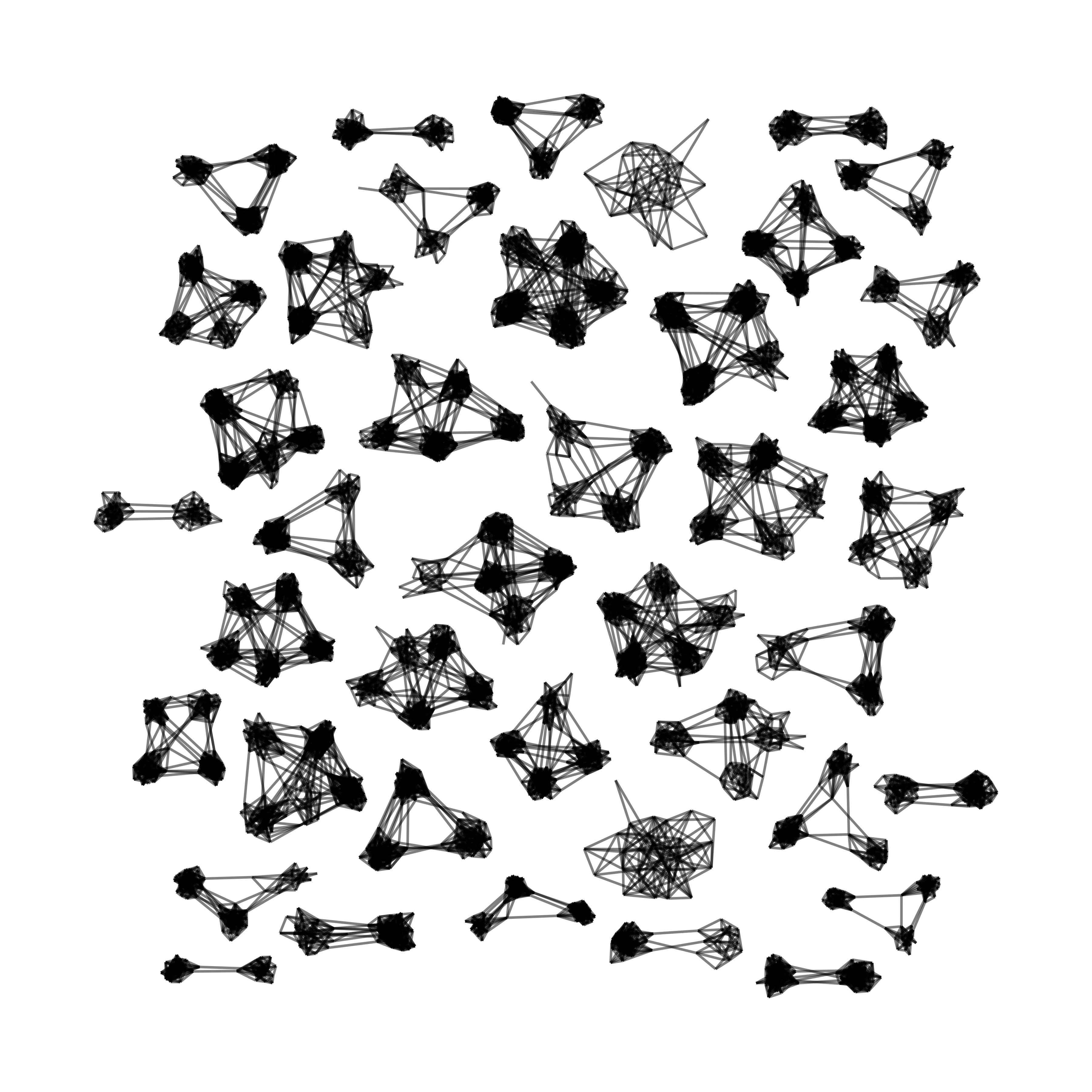
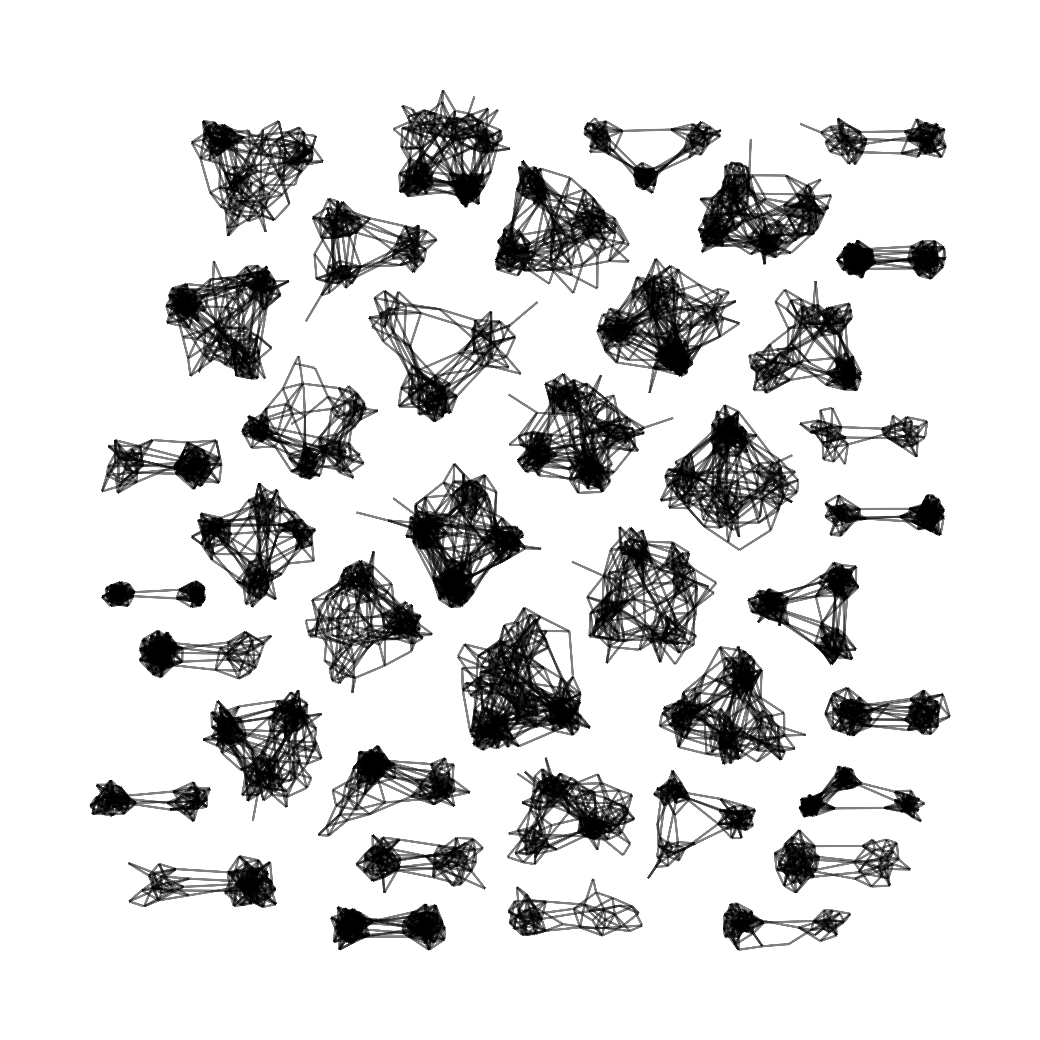
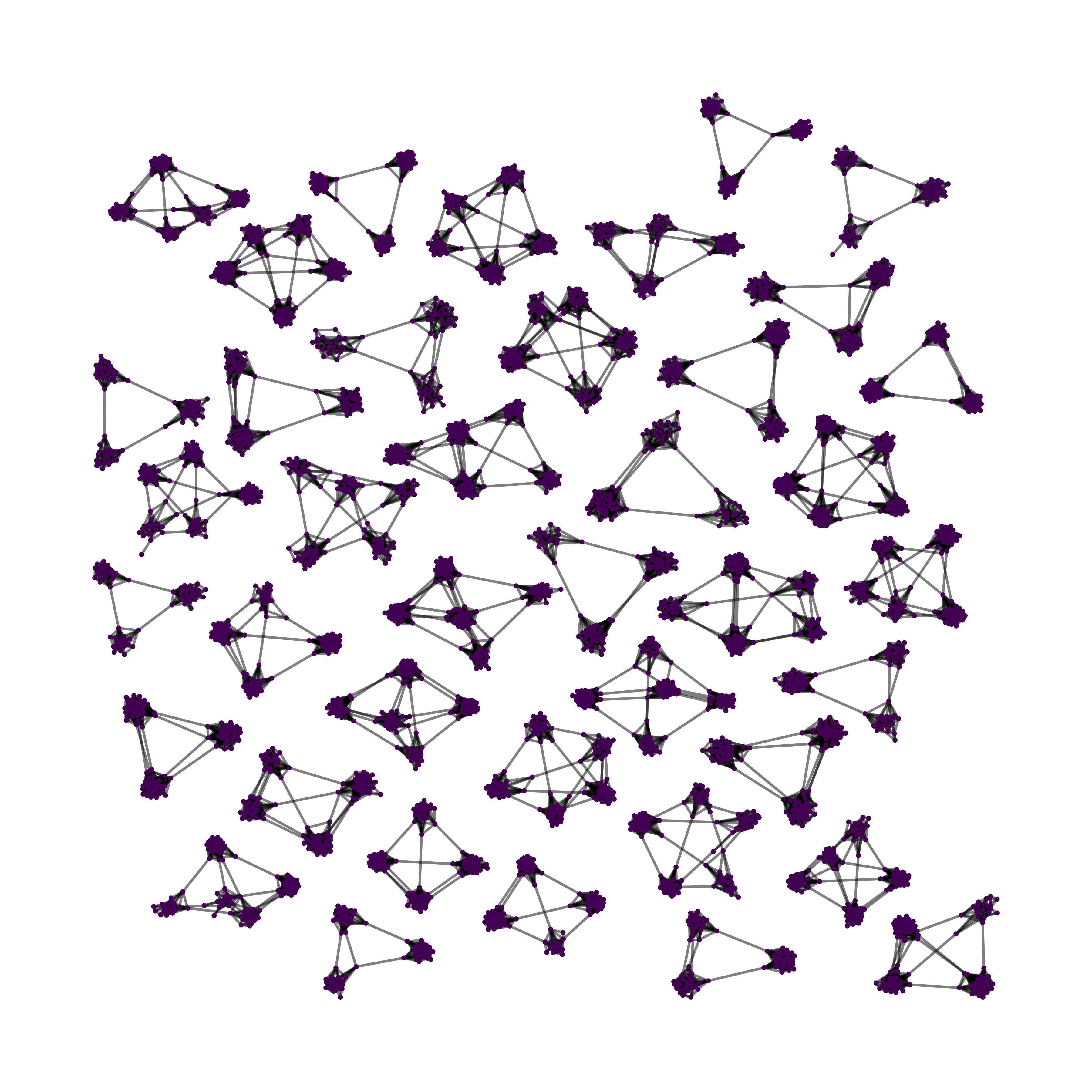
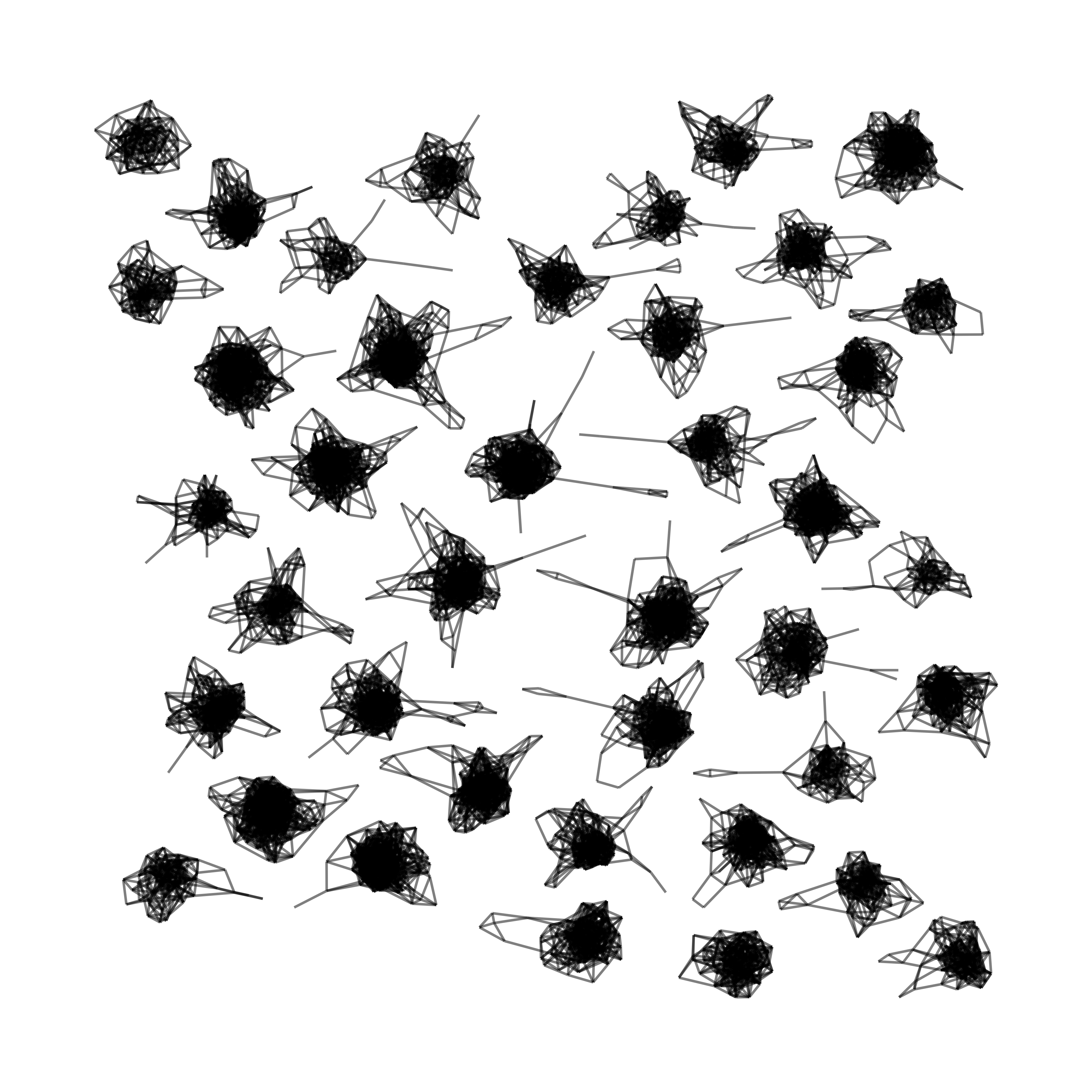
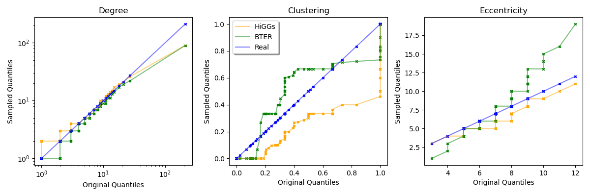
For the SBM dataset we sample 40 graphs (the size of the prescribed test-set) using DiGress, BTER and HiGGs. BTER graphs are fit on each individual test-set graph. For the Cora and Facebook Page-Page datasets we use HiGGs and BTER to sample one large graph. Where multiple connected components are produced we take only the largest. Aggregate results can be found in the supplemental material. $N_{C}$ denotes the number of communities found under Louvain segmentation, and $|C|_{med}$ the median size of those communities. Maximum Mean Discrepancy (MMD) scores can be found in Table 1. Details of the measured quantities used for these scores is found in the supplemental material. We exclude values where sample sizes of measured quantities are small. Quantile-Quantile (QQ) plots and visualisations of sampling results can be found in the supplemental material for the Facebook graph and in the supplemental material for the Cora graph and SBM dataset.

Table 1: MMD scores for models applied to each dataset. “Communities” denotes MMD calculated on communities re-sampled with Louvain partitioning.

		Nodes	Degree	Clustering	Eccentricity	Spectre
SBM	HiGGs	$\numprint{0.547}$	$\numprint{0.286}$	$\numprint{0.411}$	$\numprint{0.0401}$	$\numprint{0.314}$
	DiGress	$\numprint{0.407}$	$\numprint{0.267}$	$\numprint{0.168}$	$\numprint{0.0193}$	$\numprint{0.195}$
	BTER	$\numprint{0.088}$	$\numprint{0.189}$	$\numprint{1.07}$	$\numprint{0.051}$	$\numprint{0.311}$
Cora	HiGGs	–	$\numprint{0.254}$	$\numprint{0.958}$	$\numprint{0.273}$	–
Cora	BTER	–	$\numprint{0.439}$	$\numprint{0.281}$	$\numprint{0.00364}$	–
Cora Communities	HiGGs	$\numprint{0.662}$	$\numprint{0.069}$	$\numprint{0.451}$	$\numprint{0.0135}$	$\numprint{0.100}$
Cora Communities	BTER	$\numprint{0.598}$	$\numprint{0.290}$	$\numprint{0.417}$	$\numprint{0.00942}$	$\numprint{0.100}$
Facebook	HiGGs	–	$\numprint{2.00}$	$\numprint{0.904}$	$\numprint{0.229}$	–
Facebook	BTER	–	$\numprint{1.31}$	$\numprint{0.402}$	$\numprint{0.368}$	–
Facebook Communities	HiGGs	$\numprint{0.744}$	$\numprint{0.0436}$	$\numprint{0.0918}$	$\numprint{0.00638}$	$\numprint{0.045}$
Facebook Communities	BTER	$\numprint{0.620}$	$\numprint{0.104}$	$\numprint{0.481}$	$\numprint{0.0139}$	$\numprint{0.108}$

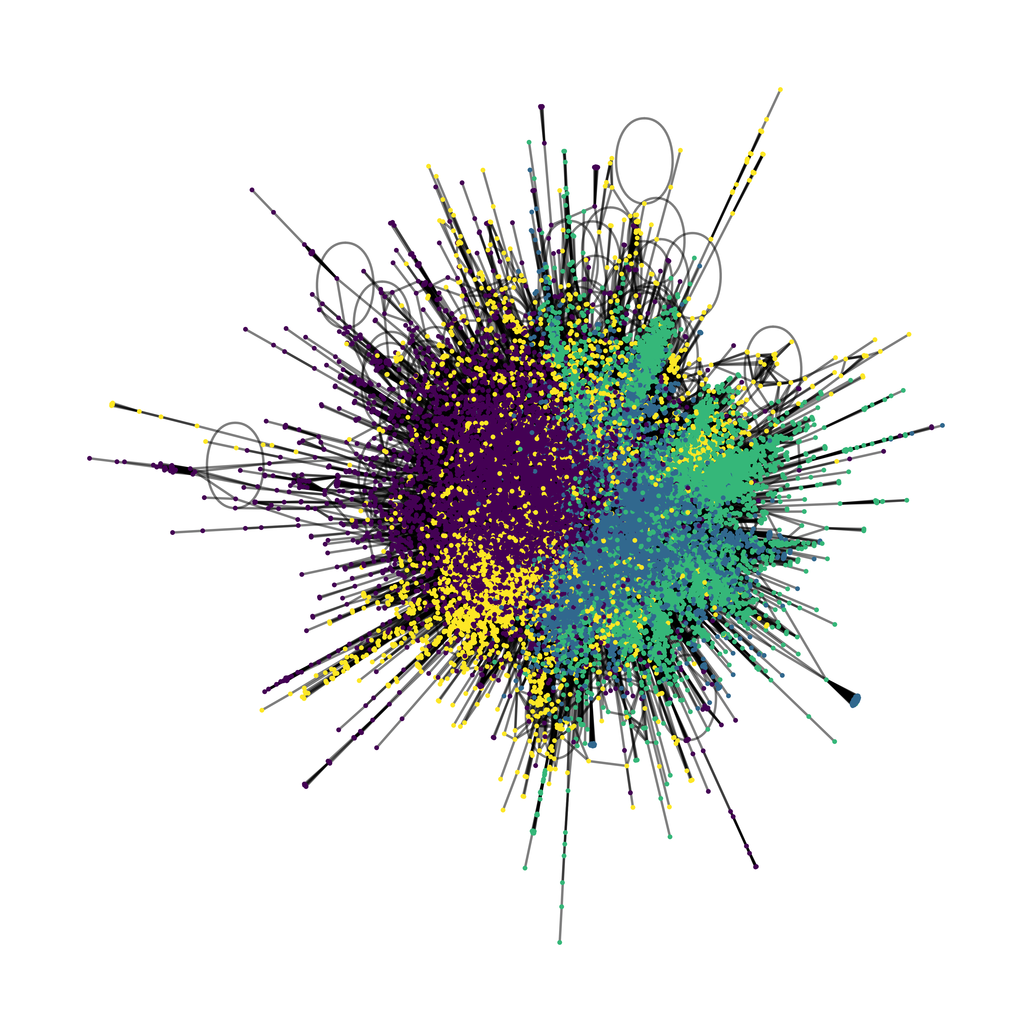
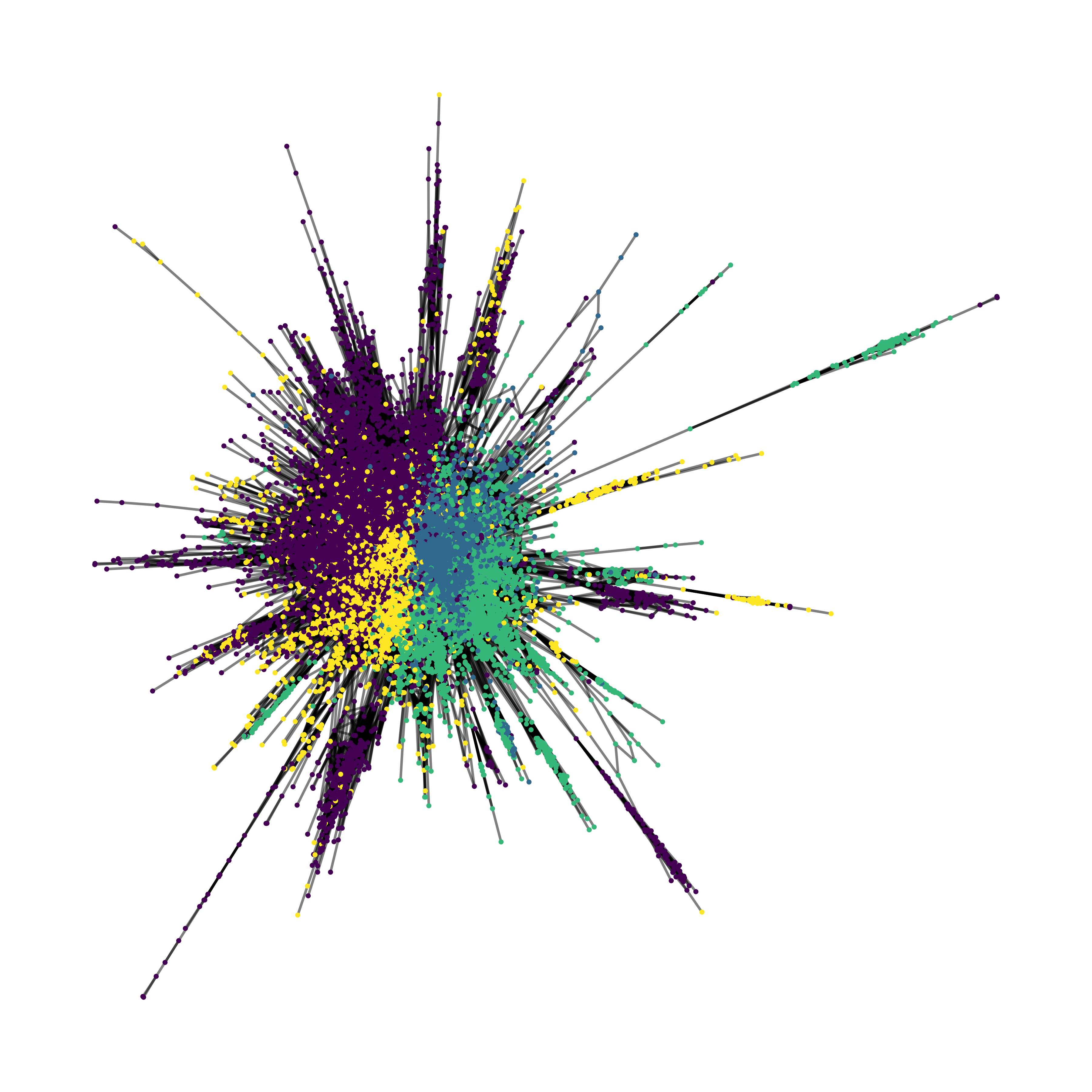
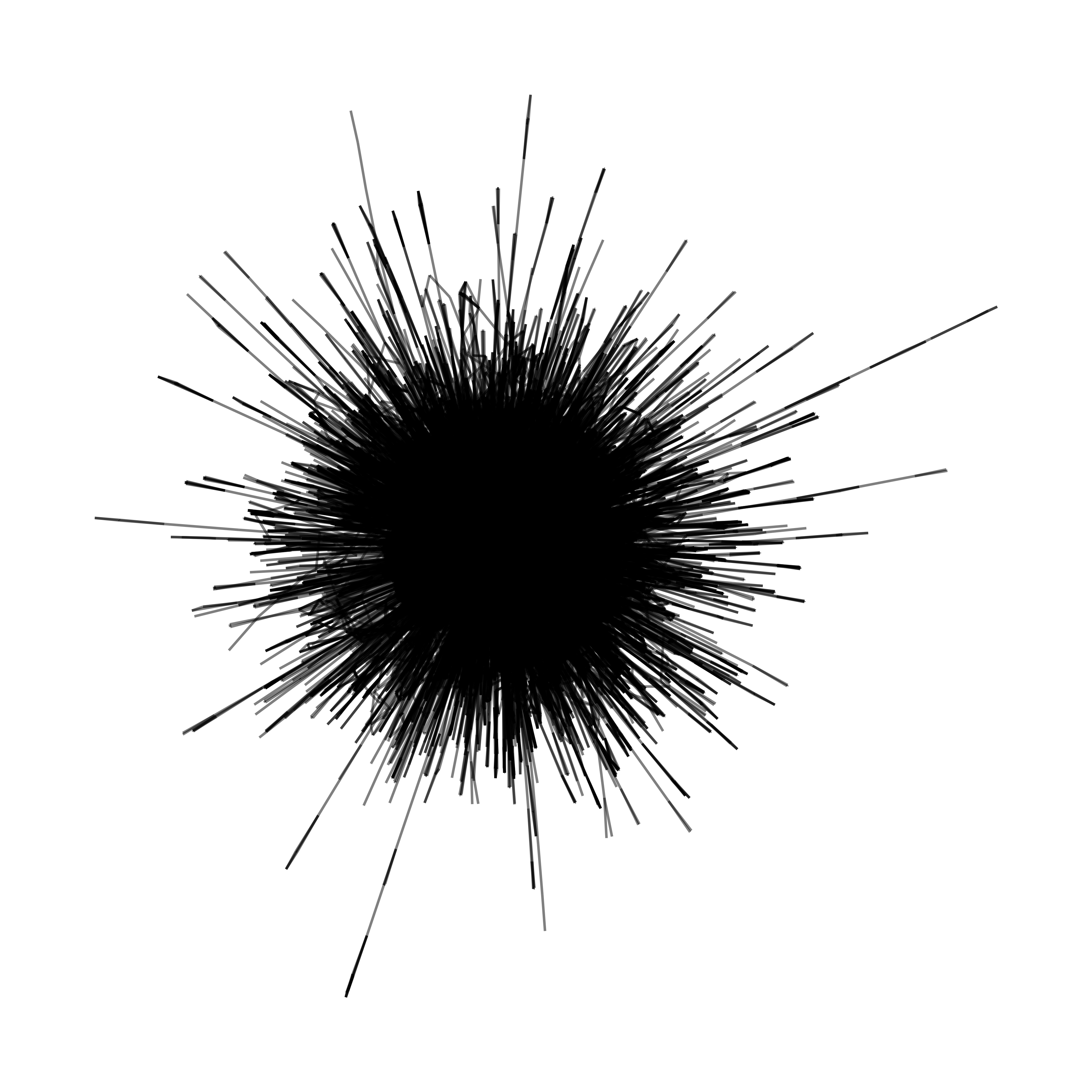
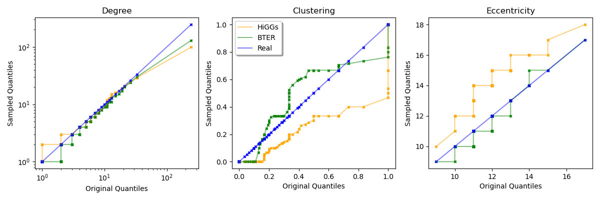
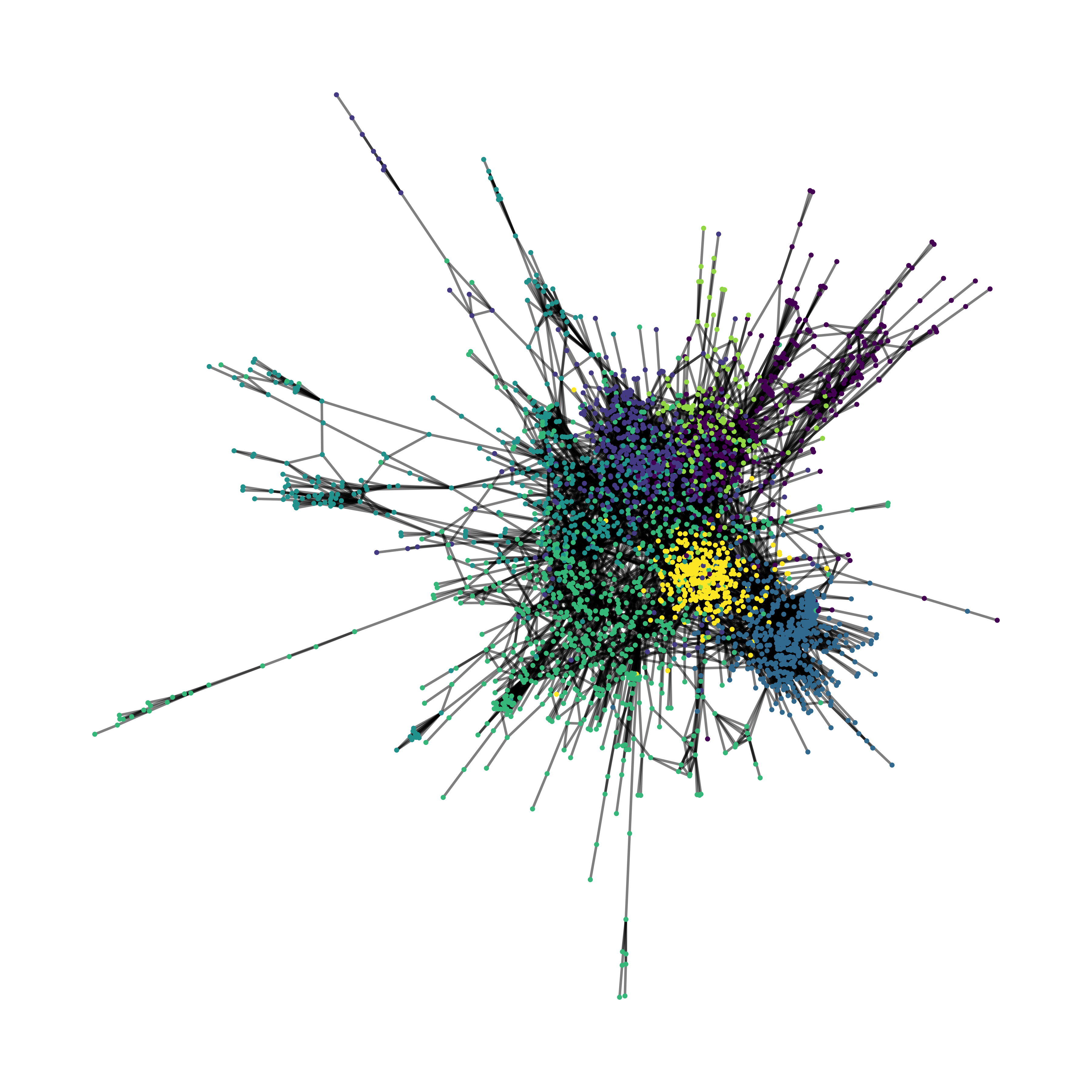
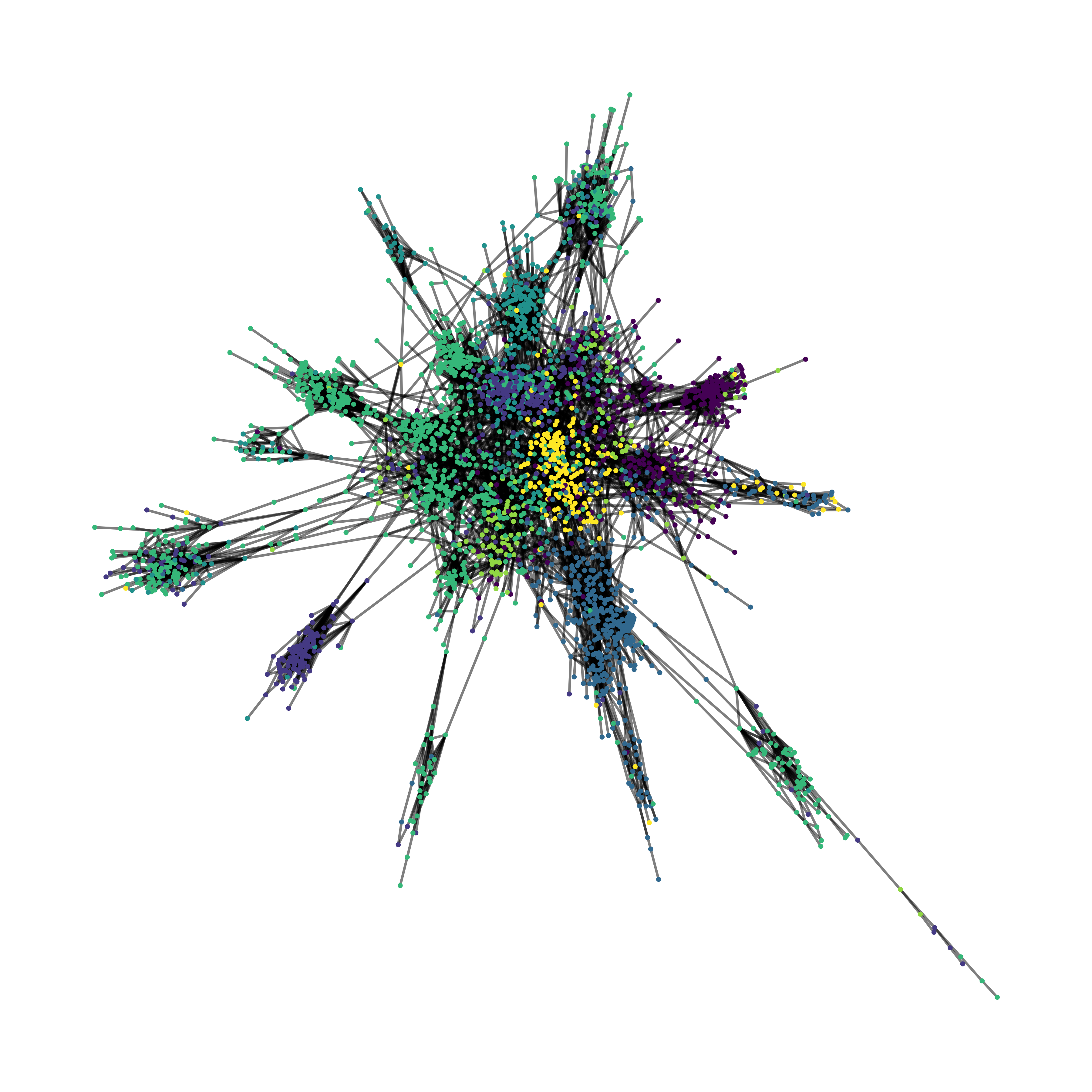
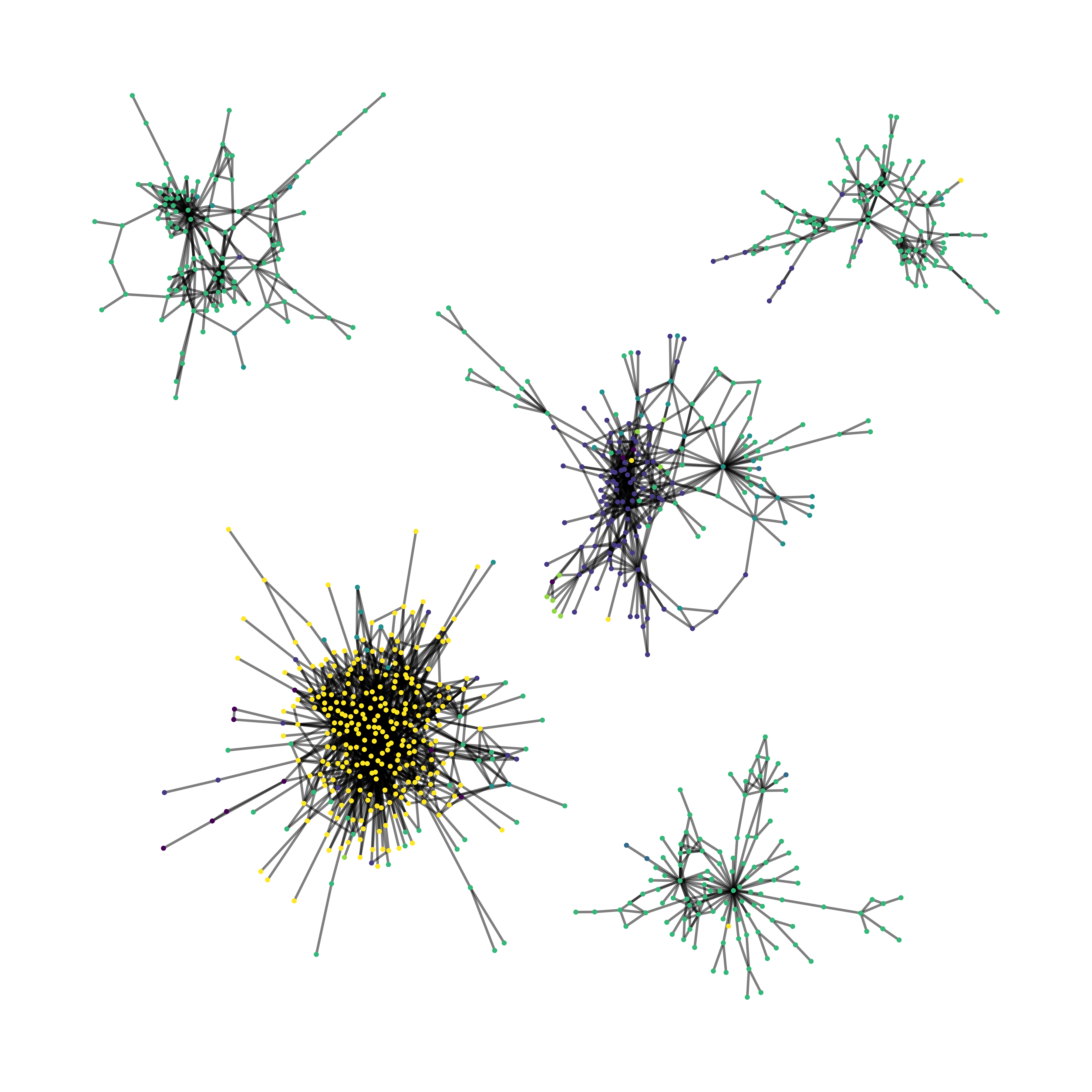
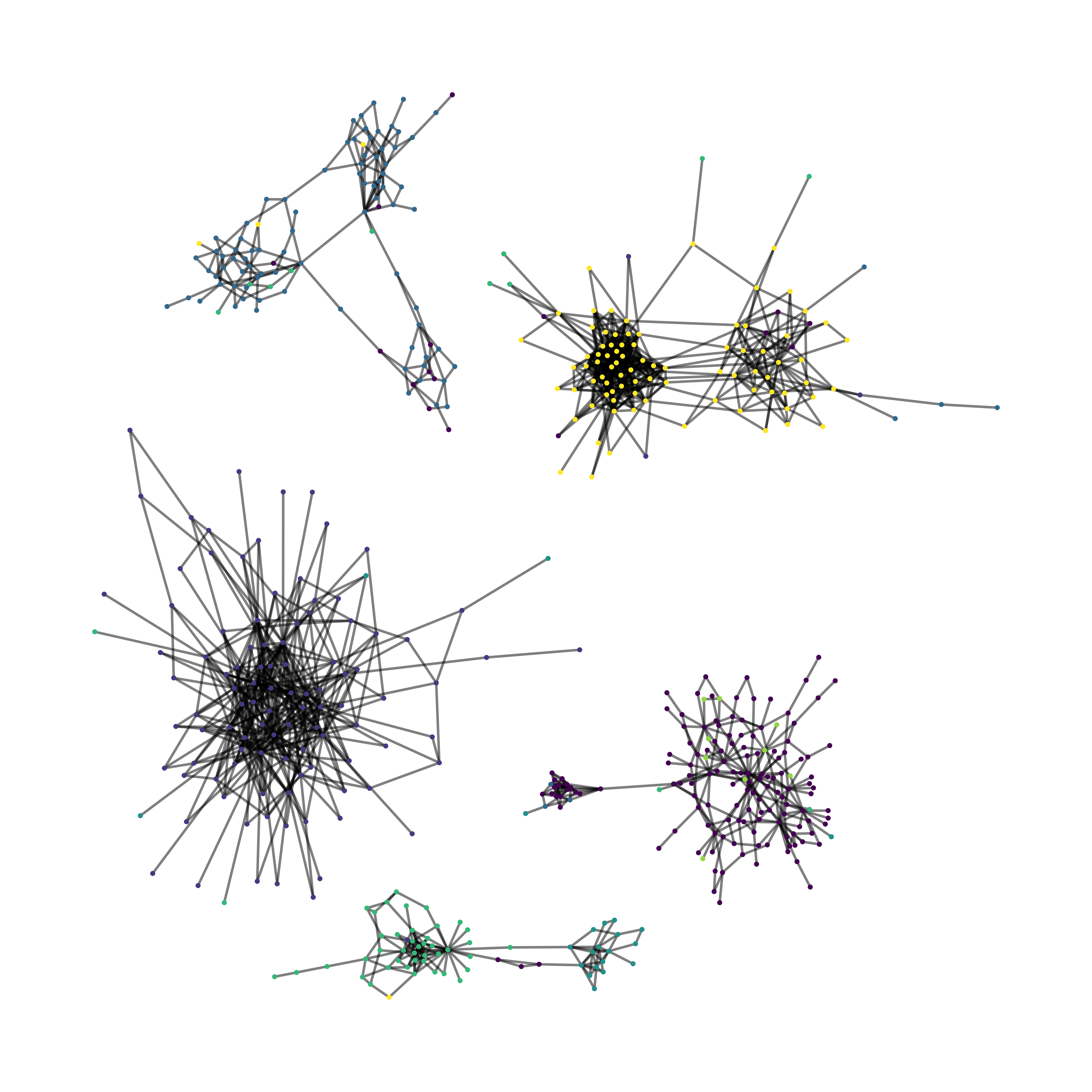
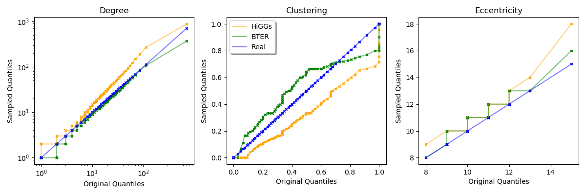
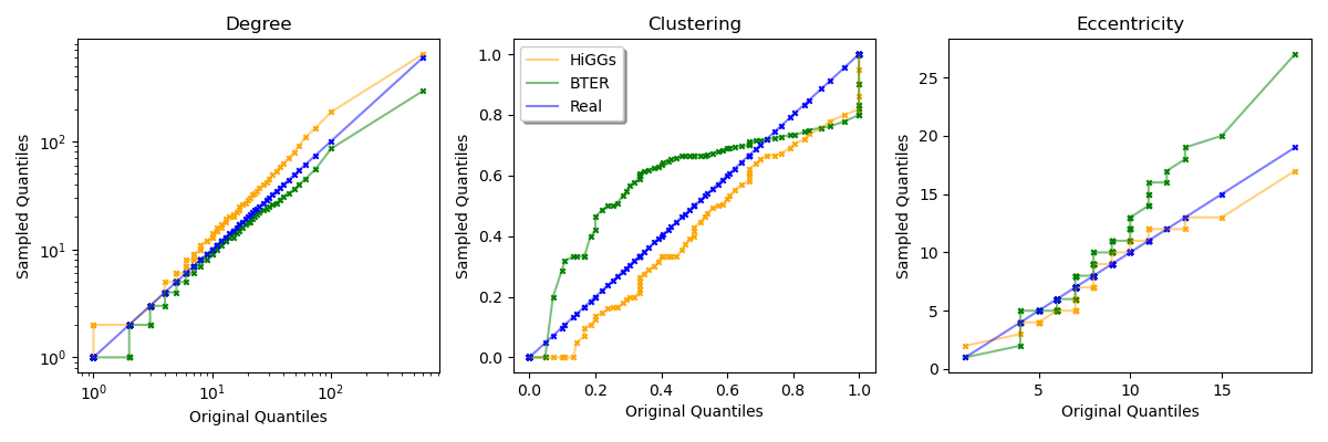
Application of measurements and MMD to graphs of this scale is unlikely to properly assess generative performance on the small-scale. To this end we apply Louvain community detection again, with a resolution of 1, to both the original Cora and Facebook graphs and their sampled counterparts from HiGGs and BTER. Following this partitioning we calculate MMD scores on the resulting real and synthetic partitions. QQ plots and visualisations of partitions are found in Figure 9 for the Facebook graphs and in the supplemental material for the Cora graphs.

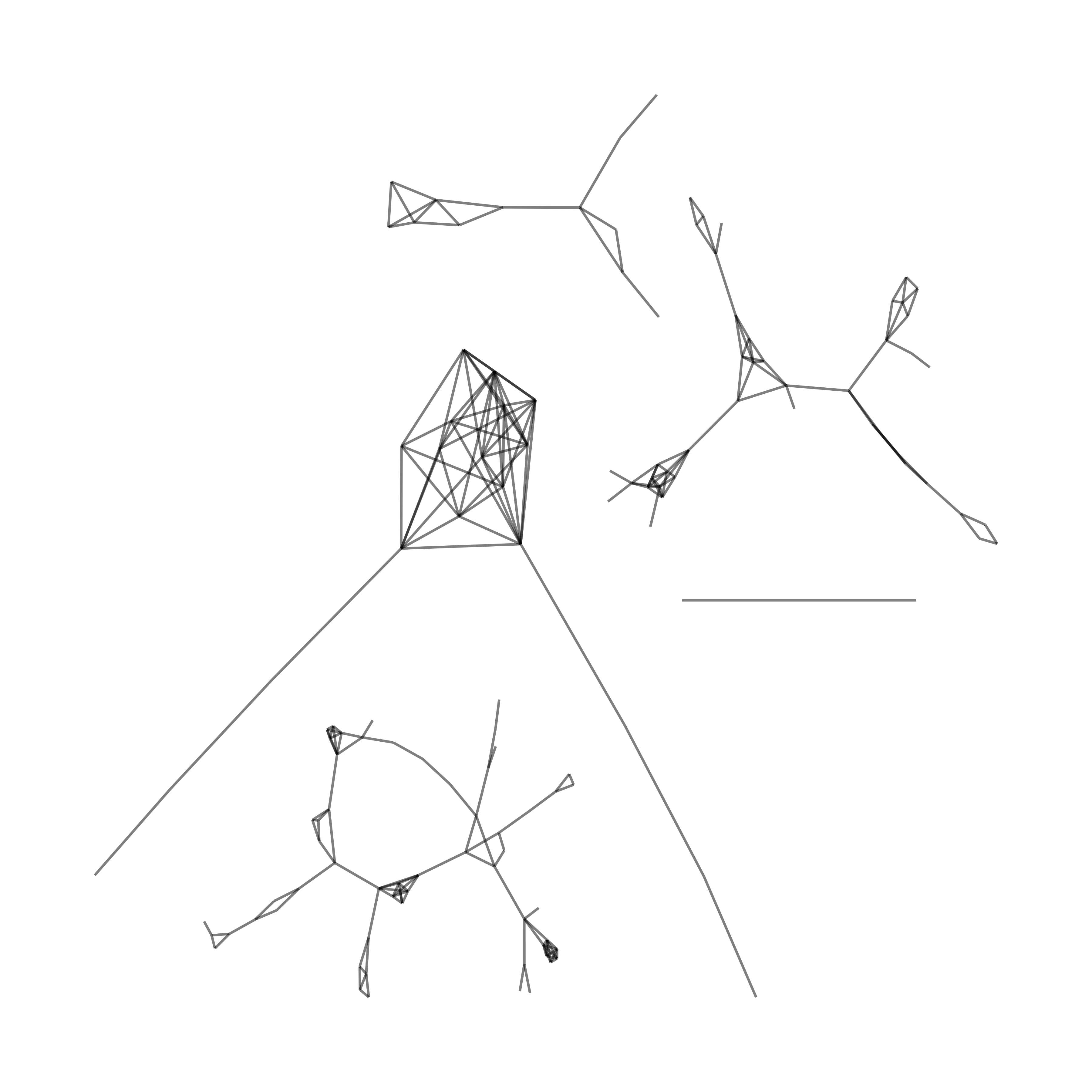
BTER fails to replicate the essential structure of the SBM graphs, as seen in Figure 1, but as expected does achieve close matches on clustering and degree. It seems that HiGGs consistently produces higher degree and clustering values than in the original SBM graphs. Interestingly, DiGress appears to do the inverse, consistently producing lower degree and clustering values, albeit with more realistic clustering values at higher ranges than HiGGs. Performance degradation from using DiGress in HiGGs, instead of by itself, is not as significant as we might have expected.

4.2.1 Large Graphs

We find that BTER produces a reasonable number of connected components, with using the largest component resulting in the lower number of nodes. On whole graph measurements we find that BTER slightly outperforms HiGGs, but not consistently on the same metrics across datasets. The exception, where HiGGs produces consistently more realistic distributions than BTER, is when Louvain segmentation is applied. Here BTER produces many smaller partitions, indicating many high-modularity groupings of nodes, instead of the larger groupings produced by the original graphs and HiGGs. On both the Cora and Facebook graphs BTER produces more realistic clustering coefficient distributions than HiGGs. On these large graphs HiGGs produces nodes with lower clustering coefficients than the original graph and BTER does the opposite.

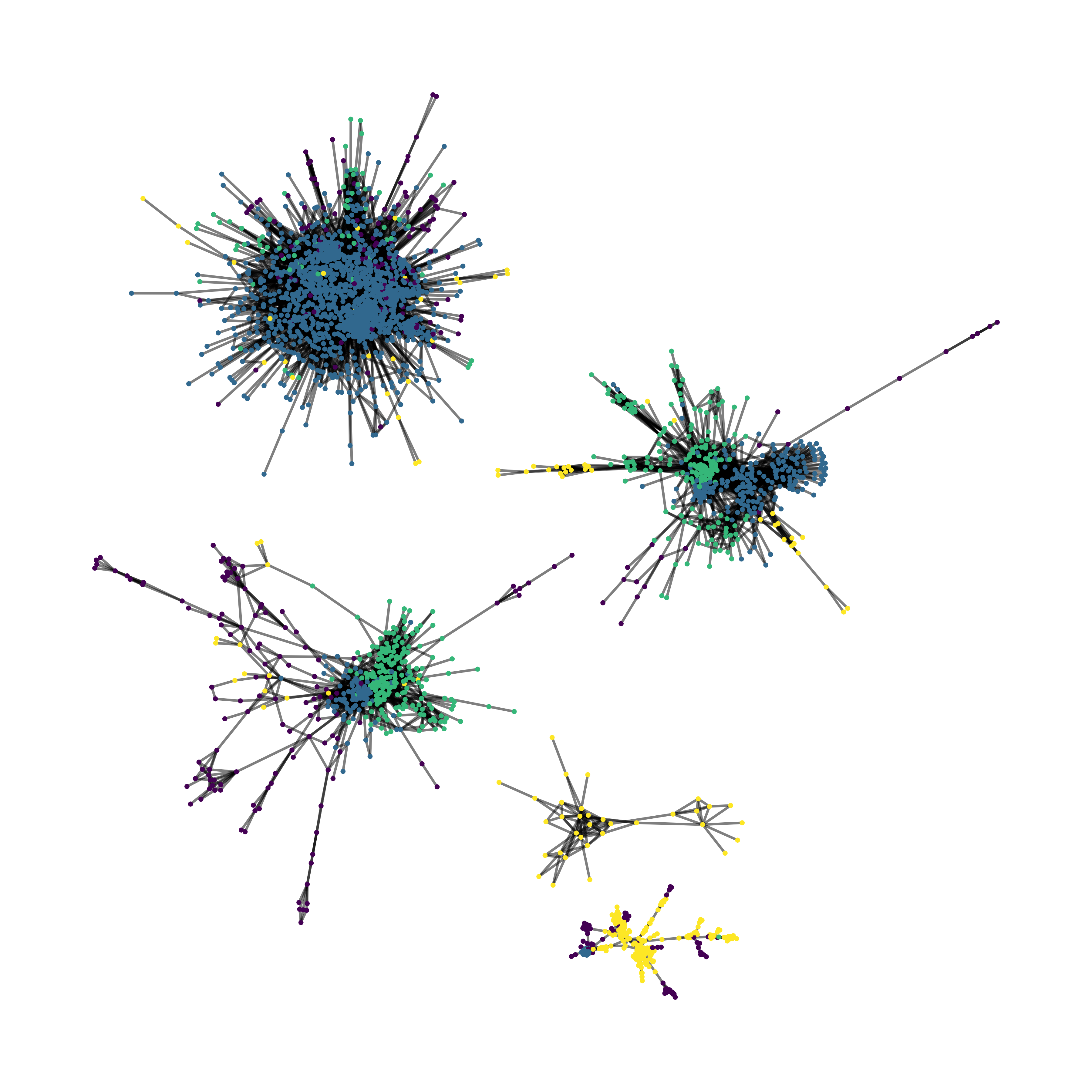
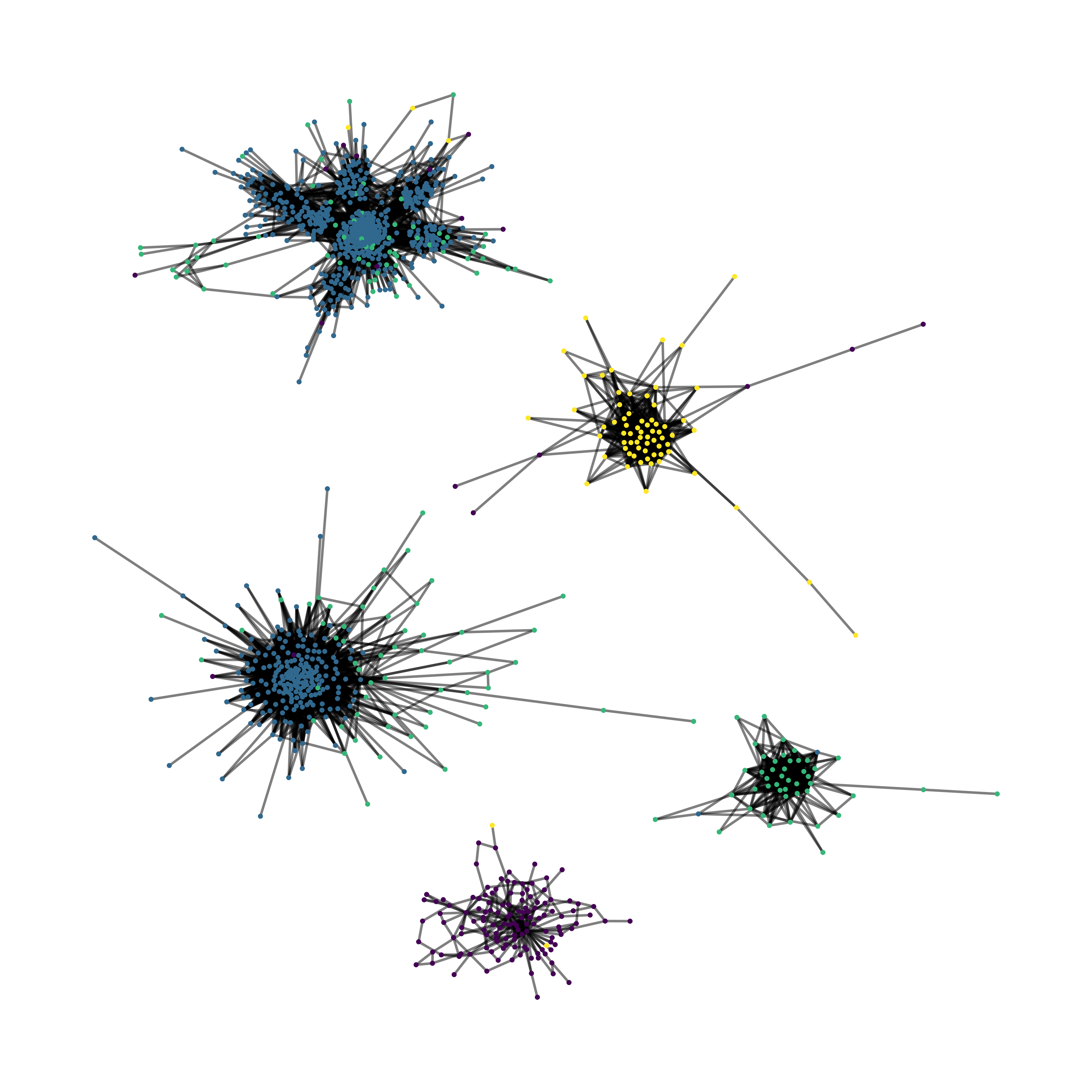
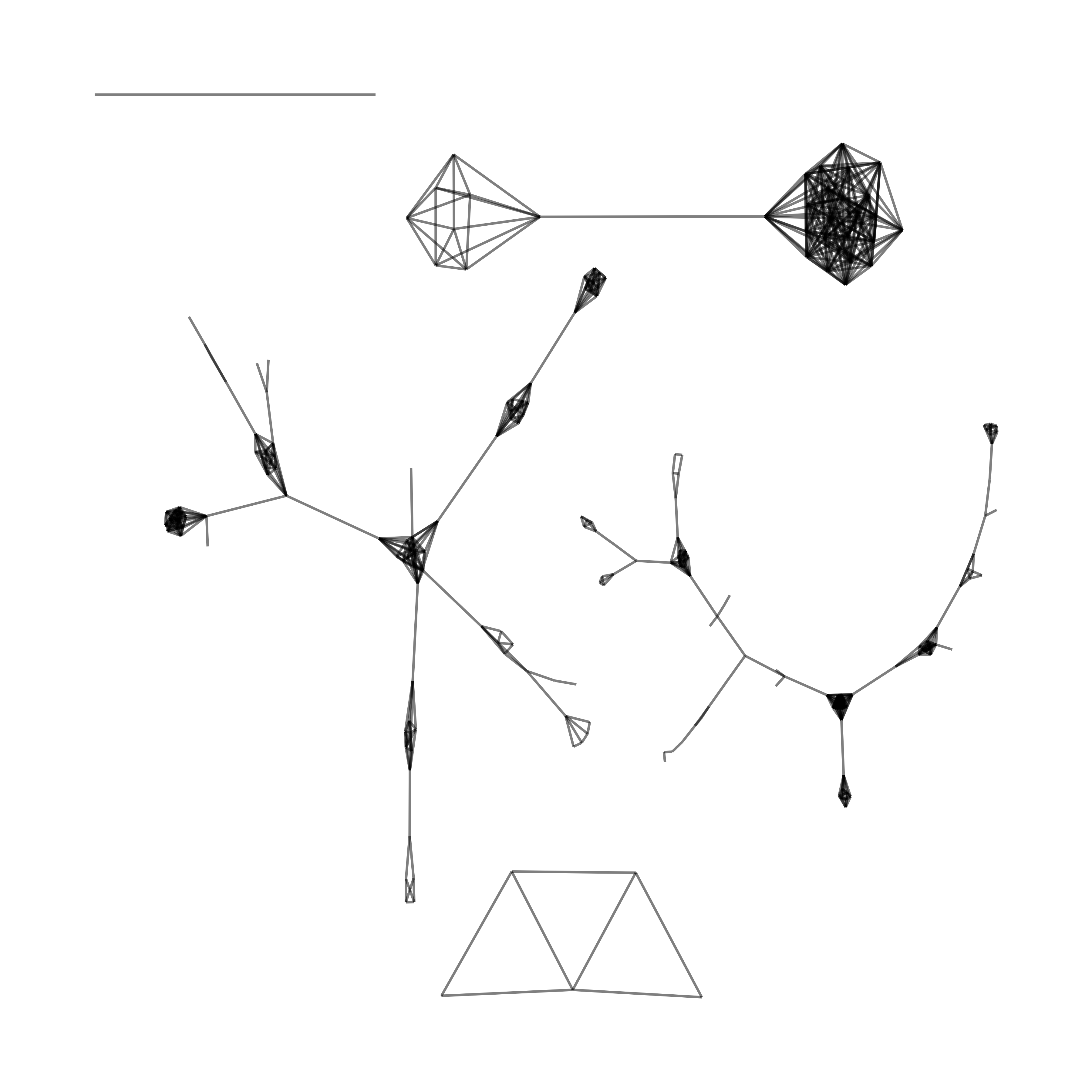
Degree distributions produced by HiGGs are much closer to the original on the Cora graph than the Facebook graph. Indeed on the Facebook data HiGGs over-produces high-degree nodes to the extent that the sampled graph’s overall density is nearly double that of the original. MMD scores on Louvain communities from the Facebook and Cora graphs show stronger performance on a small scale from HiGGs than BTER. This is particularly true on the Facebook dataset, where HiGGs communities out-perform BTER communities on all except the distribution of community sizes Visualisation of the communities shows clearly the prioritisation by BTER of clustering coefficients over overall structure. The Spectre MMD score in Table 1 confirms these conclusions.

5 Discussion

We find that performance does drop on the SBM dataset compared to DiGress, with HiGGs producing nodes with higher degrees and lower clustering coefficients, but this drop in quality is not massive. At this scale of graph HiGGs is on-par with BTER but visualisation (see supplemental material) indicates that the essential nature of these graphs has not been captured by BTER.

An important consideration when discussing the findings of this work is that neither benchmark model (BTER and DiGress) is necessarily a fair comparison. Due to the in-memory costs of DiGress (and other GNN models) graphs of the scale used in our experiments simply cannot be produced. It is arguable that rule-based models do not have the same aim as GNN models or HiGGs. Rule-based models generally attempt to re-construct a graph, often taking a certain distribution like degree (as in BTER) as an input parameter, and act as an exploration of mathematical modelling more than as a generative task. This means that on quantitative metrics like MMD they often perform very strongly, but on characteristics more difficult to express through metrics, they tend to fail.

We find that on the small scale, through application of Louvain partitioning, HiGGs has out-performed BTER. This includes on the clustering coefficients specifically targeted by BTER, with clustering coefficients on the community scale produced by BTER consistently too high. Visualisation of communities corroborates this, with BTER producing many triangles, instead of many-node patterns. Conversely our HiGGs implementation performs much better in this regard. Given that MMD scores and aggregate metrics both rely on simple node-level measurements on graphs of this scale they may not be sufficiently expressive. Issues with MMD, even on the few-hundred-node scale, are discussed more specifically in O’Bray et al. [16]. We further discuss our assumptions and threats to validity in the supplemental material.

6 Conclusion

In this work, we propose HiGGs as a framework for generating large graphs. We implement HiGGs using DiGress [22], a recent graph diffusion model with the capacity to consider node attribution and conditional generation, and for inter- $h_{1}$ edge sampling we implement the first edge-predictive-diffusion model as a variant of DiGress. This is, to our knowledge, the first deep-learning based method to produce graphs of tens of thousands of nodes. Further, HiGGs is able to do so with categorical node and edge attributes, with our generated graphs up to 200 times larger than those in the original DiGress paper. Using this HiGGs implementation, we demonstrate that on the benchmark SBM dataset performance is not significantly degraded from using DiGress by itself. Comparison to BTER, a rule-based method, shows that our HiGGs implementation out-performs BTER on small-scale measurement of large sampled graphs. However, due to BTER’s use of a prescribed degree distribution, BTER out-performs our HiGGs implementation when considering whole-graph node metric distributions.

While the implementation of HiGGs presented here is viable for social networks, and possibly other applications, future work could focus on a few key areas. Firstly, whether HiGGs is improved compared to our implementation here by using different partitioning algorithms and generative models, in particular a more efficient edge sampling model. Secondly, an improved edge-sampling stage, that considers previous edge-samplings, might significantly improve results and allow extension to geometric or quasi-geometric graphs like molecules. We hope that domain experts in fields such as chemistry develop their own task-specific implementations.

References

[1]
Boitmanis et al. [2006] Krists Boitmanis, Karlis Freivalds, Peteris Lediņš, and Rudolfs Opmanis. 2006. Fast and simple approximation of the diameter and radius of a graph. In Lecture Notes in Computer Science (including subseries Lecture Notes in Artificial Intelligence and Lecture Notes in Bioinformatics). Vol. 4007 LNCS. Springer Verlag, 98–108. https://doi.org/10.1007/11764298{\_}9/COVER
Bojchevski et al. [2018] Aleksandar Bojchevski, Oleksandr Shchur, Daniel Zugner, and Stephan Gunnemann. 2018. NetGAN: Generating Graphs via random walks. In Proceedings of the 35th International Conference on Machine Learning (ICML), Vol. 2. International Machine Learning Society (IMLS), Stockholm, 973–988.
Chakrabarti et al. [2004] Deepayan Chakrabarti, Yiping Zhan, and Christos Faloutsos. 2004. R-MAT: A Recursive Model for Graph Mining. In Proceedings of the 2004 SIAM International Conference on Data Mining. Society for Industrial and Applied Mathematics, Philadelphia, PA, 442–446. https://doi.org/10.1137/1.9781611972740.43
Chen et al. [2022] Xiaohui Chen, Yukun Li, Aonan Zhang, and Li-ping Liu. 2022. NVDiff: Graph Generation through the Diffusion of Node Vectors. (Nov. 2022). http://arxiv.org/abs/2211.10794
Davies and Ajmeri [2022] Alex Davies and Nirav Ajmeri. 2022. Realistic Synthetic Social Networks with Graph Neural Networks. (Dec. 2022). http://arxiv.org/abs/2212.07843
De Meo et al. [2011] Pasquale De Meo, Emilio Ferrara, Giacomo Fiumara, and Alessandro Provetti. 2011. Generalized Louvain method for community detection in large networks. In Proceedings of the International Conference on Intelligent Systems Design and Applications (ISDA), Vol. abs/1108.1502. 88–93. https://doi.org/10.1109/ISDA.2011.6121636
Erdos and Renyi [1960] P. Erdos and A. Renyi. 1960. On the Evolution of Random Graphs. Trans. Amer. Math. Soc. 286 (Nov. 1960), 257–274.
Gilmer et al. [2017] Justin Gilmer, Samuel S. Schoenholz, Patrick F. Riley, Oriol Vinyals, and George E. Dahl. 2017. Neural Message Passing for Quantum Chemistry. In Proceedings of the 34th International Conference on Machine Learning (ICML), Vol. 3. International Machine Learning Society (IMLS), 2053–2070. https://doi.org/10.48550/arxiv.1704.01212
Guo and Zhao [2022] Xiaojie Guo and Liang Zhao. 2022. A Systematic Survey on Deep Generative Models for Graph Generation. arXiv e-print 1, 1 (2022), 1–25. https://doi.org/10.48550/arXiv.2007.06686
Ho et al. [2020] Jonathan Ho, Ajay Jain, and Pieter Abbeel. 2020. Denoising diffusion probabilistic models. In Advances in Neural Information Processing Systems, Vol. 2020-December. Curran Associates, Inc., Online, 6840–6851.
Huang et al. [2022] Han Huang, Leilei Sun, Bowen Du, Yanjie Fu, and Weifeng Lv. 2022. GraphGDP: Generative Diffusion Processes for Permutation Invariant Graph Generation. In Proceedings of the IEEE International Conference on Data Mining (ICDM). IEEE Computer Society, Los Alamitos, 201–210. https://doi.org/10.48550/arxiv.2212.01842
Jin et al. [2020] Wengong Jin, Regina Barzilay, and Tommi Jaakkola. 2020. Hierarchical Generation of Molecular Graphs using Structural Motifs. In Proceedings of the 37th International Conference on Machine Learning. JMLR.org, Online, Article 449, 10 pages. https://doi.org/10.5555/3524938.3525387
Liao et al. [2019] Renjie Liao, Yujia Li, Yang Song, Shenlong Wang, Will Hamilton, David K Duvenaud, Raquel Urtasun, and Richard Zemel. 2019. Efficient Graph Generation with Graph Recurrent Attention Networks. In Advances in Neural Information Processing Systems 32 (NeurIPS 2019), H Wallach, H Larochelle, A Beygelzimer, F d Alché-Buc, E Fox, and R Garnett (Eds.), Vol. 32. Curran Associates, Inc., Vancouver, Canada, 1–11. https://proceedings.neurips.cc/paper/2019/file/d0921d442ee91b896ad95059d13df618-Paper.pdf
Martinkus et al. [2022] Karolis Martinkus, Andreas Loukas, Nathanaël Perraudin, and Roger Wattenhofer. 2022. SPECTRE: Spectral Conditioning Helps to Overcome the Expressivity Limits of One-shot Graph Generators. In Proceedings of the 39th International Conference on Machine Learning, Vol. 162. PMLR, Honolulu, Hawaii, 15159–15179. https://doi.org/10.48550/ARXIV.2204.01613
O’Bray et al. [2021] Leslie O’Bray, Max Horn, Bastian Rieck, and Karsten Borgwardt. 2021. Evaluation Metrics for Graph Generative Models: Problems, Pitfalls, and Practical Solutions. In ICLR 2022 - 10th International Conference on Learning Representations.
Rozemberczki et al. [2021] Benedek Rozemberczki, Carl Allen, and Rik Sarkar. 2021. Multi-Scale attributed node embedding. Journal of Complex Networks 9, 2 (May 2021), 1–22. https://doi.org/10.1093/comnet/cnab014
Ščupáková et al. [2019] Klára Ščupáková, Vasilis Terzopoulos, Saurabh Jain, Dirk Smeets, and Ron M.A. Heeren. 2019. A patch-based super resolution algorithm for improving image resolution in clinical mass spectrometry. Scientific Reports 9, 1 (Feb. 2019), 1–11. https://doi.org/10.1038/s41598-019-38914-y
Sen et al. [2008] Prithviraj Sen, Galileo Mark Namata, Mustafa Bilgic, Lise Getoor, Brian Gallagher, and Tina Eliassi-Rad. 2008. Collective classification in network data. AI Magazine 29, 3 (Sept. 2008), 93–106. https://doi.org/10.1609/aimag.v29i3.2157
Seshadhri et al. [2012] C. Seshadhri, Tamara G. Kolda, and Ali Pinar. 2012. Community structure and scale-free collections of Erdos-Rényi graphs. Physical Review E - Statistical, Nonlinear, and Soft Matter Physics 85, 5 (May 2012), 056109. https://doi.org/10.1103/PhysRevE.85.056109
Simonovsky and Komodakis [2018] Martin Simonovsky and Nikos Komodakis. 2018. GraphVAE: Towards Generation of Small Graphs Using Variational Autoencoders. In Proceedings of the International Conference on Artificial Neural Networks (ICANN). Springer, Rhodes, 412–422. http://arxiv.org/abs/1802.03480
Vignac et al. [2023] Clement Vignac, Igor Krawczuk, Antoine Siraudin, Bohan Wang, Volkan Cevher, and Pascal Frossard. 2023. DiGress: Discrete Denoising diffusion for graph generation. (2023). https://openreview.net/forum?id=UaAD-Nu86WX
Wang et al. [2017] Hongwei Wang, Jia Wang, Jialin Wang, Miao Zhao, Weinan Zhang, Fuzheng Zhang, Xing Xie, and Minyi Guo. 2017. GraphGAN: Graph Representation Learning with Generative Adversarial Nets. In Proceedings Of the 32nd AAAI Conference on Artificial Intelligence (AAAI). AAAI Press, New Orleans, 2508–2515. http://arxiv.org/abs/1711.08267
Watts and Strogatz [1998] Duncan J. Watts and Steven H. Strogatz. 1998. Collective dynamics of ‘small-world’ networks. Nature 1998 393:6684 393, 6684 (June 1998), 440–442. https://doi.org/10.1038/30918
Xie et al. [2019] Saining Xie, Alexander Kirillov, Ross Girshick, and Kaiming He. 2019. Exploring Randomly Wired Neural Networks for Image Recognition. In Proceedings of the IEEE/CVF International Conference on Computer Vision (ICCV). IEEE Computer Society, Seoul, 1284–1293. https://doi.org/10.1109/ICCV.2019.00137
You et al. [2018] Jiaxuan You, Rex Ying, Xiang Ren, William L. Hamilton, and Jure Leskovec. 2018. GraphRNN: Generating Realistic Graphs with Deep Auto-regressive Models. In Proceedings of the 35th International Conference on Machine Learning (ICML), Vol. 13. International Machine Learning Society (IMLS), 9072–9081.
Zhang et al. [2021] Liming Zhang, Liang Zhao, Shan Qin, Dieter Pfoser, and Chen Ling. 2021. TG-GAN: Continuous-time temporal graph deep generative models with time-validity constraints. In Proceedings of the World Wide Web Conference. ACM, Online, 2104–2116. https://doi.org/10.1145/3442381.3449818
Zhang et al. [2022] Ziwei Zhang, Peng Cui, and Wenwu Zhu. 2022. Deep Learning on Graphs: A Survey. IEEE Transactions on Knowledge and Data Engineering 34, 1 (Jan. 2022), 249–270. https://doi.org/10.1109/TKDE.2020.2981333
Zhu et al. [2022] Yanqiao Zhu, Yuanqi Du, Yinkai Wang, Yichen Xu, Jieyu Zhang, Qiang Liu, and Shu Wu. 2022. A Survey on Deep Graph Generation: Methods and Applications. ArXiv 1, 1 (March 2022), 1–14. https://doi.org/10.48550/arxiv.2203.06714

Appendix A Appendix

A.1 Code Availability

All code is available at https://github.com/higgs-neurips-23/HiGGs. This repository also contains scripts to download the trained models for each dataset. Model training and sampling was conducted on a single workstation computer equipped with an NVIDIA A6000 48gb GPU.

A.2 HiGGs schematic

A.3 Current Models

Table 2: Existing GNN graph generation methods. Order is listed as the worst case stated in the respective work and the maximum size of graphs

\lim(|V|)

is the highest stated in the respective work, although maximum graph size was not necessarily their primary aim. ^† indicates an order not explicitly stated in the respective work.

Model	Order	$\lim(\|V\|)$	Attribution			Conditioning
Model	Order	$\lim(\|V\|)$	Node	Edge	Graph	Conditioning
GraphVAE [21]	$N^{4}$	$\numprint{38}$	✓	✓	✓	✓
DiGress [22]	$N^{2}$	$\numprint{100}$	✓	✓	✓	✓
GraphGDP [12]	– ^†	$\numprint{399}$	✗	✗	✗	✓
NVDiff [5]	$N$	$\numprint{400}$	✓	✓	✗	✗
GraphRNN [26]	$N^{2}$	$\numprint{500}$	✗	✗	✗	✗
NetGAN [3]	– ^†	$\numprint{2810}$	✗	✗	✗	✗
GRAN [14]	$N\log(N)$	$\numprint{3530}$	✗	✗	✗	✗
HiGGs	See paper	$\numprint{22000}$	✓	✓	✓	✓

A.4 HiGGs Complexity

The size of the final sampled graph is denoted $N_{G}=|V|$ . We denote the size of the $h_{2}$ graph $N_{2}=|h_{2}|$ . $N_{1}$ is the mean size of an $h_{1}$ graph, $N_{1}=\textrm{mean}(|h_{1}|)=N_{G}/N_{2}$ . The order of DiGress is $O(N^{2})$ , which is costly. Fortunately HiGGs does not need to scale beyond a few hundred nodes in any given sampling process. Similarly our edge-predictive variant of DiGress scales $O(N^{2})$ . This means that the complexities of HiGGs, in our implementation using Louvain [7] Segmentation, DiGress, and edge-DiGress, are $O(N_{G}^{2})$ in the segmentation stage, for both time (full sampling) and memory (per item), $O(N_{2}^{2})$ in Stage One ( $h_{2}$ ), $O(N_{G}^{2}N_{2})$ (time) and $O((N_{G}/N_{2})^{2})$ (memory) for Stage Two ( $h_{1}$ ), and $O(N_{G}^{2})$ and $O((N_{G}/N_{2})^{2})$ for Stage Three ( $h_{1,i}\leftrightarrow h_{1,j}$ ). The maximum memory requirement of edge-sampling is likely the limiting factor, because the largest graphs passed to this model are double that of the largest from $h_{1}$ .

The order of HiGGs varies by stage (see above). The size of the final sampled graph is denoted $N_{G}=|V|$ . We denote the size of the $h_{2}$ graph $N_{2}=|h_{2}|$ , ie the cardinality of its node-set. Similarly $N_{1}$ is the mean size of an $h_{1}$ graph, $N_{1}=\textrm{mean}(|h_{1}|)$ . The number of edges in $h_{2}$ is $E_{2}=|E_{h_{2}}|$ . The order of each stage is necessarily very dependent on the order of the generative model being used. We denote the order of an arbitrary model as $O(N^{x,y,z})$ with $x,y,z$ an unknown (assumed polynomial) complexity for the models in Stage One, Two and Three respectively. Training complexities for each stage simply inherit from the model, ie each stage has order $O(N_{\textrm{stage}}^{i})$ .

The order of $h_{2}$ sampling simply inherits the order of the generative model, ie $O(h_{2})=O(N_{2}^{x})$ . An $h_{1}$ graph is sampled for each node in the proceeding $h_{2}$ graph, so Stage 2 has sampling time complexity $O(h_{1})=O(N_{2}N_{1}^{y})$ . We can expect an average community size dependent on the size of the final sampled graph, so $N_{1}=N_{G}/N_{2}$ , and $O(h_{1})=O(N_{G}^{y}N_{2}^{y-1})$ .

The upper limit on size of graphs during the edge-sampling stage is double those from $h_{1}$ . The number of samples is determined by the number of edges in $h_{2}$ , $E_{2}=\rho(N_{2}^{2}/2-N)$ , where $\rho$ is the density of edges in $h_{2}$ .

This leads to an order of $O(h_{1,i}\leftrightarrow h_{1,j})=O(N_{2}^{2}N_{1}^{z})$ . Note here however that memory capacity of the GPU used is the likely limit, as we might expect $N_{1}^{x}<<(2N_{1})^{z}$ . Using the above $N_{1}=N_{G}/N_{2}$ , this becomes $O(h_{1,i}\leftrightarrow h_{1,j})=O(N_{G}^{z}N_{2}^{2-z})$ , with the actual number of edge-prediction operations scaled linearly by $h_{2}$ edge density $\rho_{2}$ . Crucially, and unlike block-generative or motif-based models, stages two and three consist of many independent jobs, making them trivially paralellisable.

A.5 Extra Features

A.5.1 Diameter

As we are extending the number of nodes from $|V|\sim 100$ to $|V|\sim 600$ in some cases, the planarity/diameter of the graph becomes less easily expressed by DiGress. With the aim of alleviating some of these issues we implement a simple approximation for graph diameter, with the same principles as MultiBFS from Boitmanis et al. [2].

In brief summary, for a given message passing kernel size $n$ , a simple convolution without weights is given by Equation 1.

P_{n}=\sum_{i=0}^{n}A^{i}

(1)

x_{i,j}=\begin{cases}1&\text{if }j=i\\ 0&\text{otherwise}\end{cases}

(2)

x^{\prime}_{n}=P_{n}x

(3)

Selecting a random node $u$ in a graph, we construct a bit-vector $x$ with zeroes everywhere except the index of that node, as in Equation 2 for initial node index $i$ . Applying the convolution gives an updated per-node feature vector given by Equation 3. Crucially this vector is zero for nodes $v$ where a message has not reached - which means that the shortest path between the $u$ and $v$ is longer than $n$ , i.e., $SP(u,v)>n$ .

By iteratively applying a $P_{n}$ message passing convolution to the bit-vector $x$ , and tracking at what $n$ all nodes have received at least one message, we can derive the eccentricity of an individual node. We sample the eccentricities of five nodes per graph per batch then take the maximum of these as an estimate of diameter.

The advantage of this approach, as opposed to a direct diameter calculation using BFS or similar, is that it can be computed entirely through matrix operations, and on a whole batch simultaneously. This means that no movement from or to the GPU is required when it is computed during training.

A.5.2 Clustering

For a graph with adjacency matrix $A$ , which is a bit-matrix showing the existence of any edges, we can count the number of $N$ -node cycles for each node $i$ , denoted $|\theta_{n,i}|$ , using the trace of the matrix’s product with itself, i.e., for all nodes in a graph $|\theta_{n}|\in\mathbb{Z}^{|V|}$ is Equation 4.

|\theta_{n}|=\textrm{Tr}(A^{n})

(4)

C=\frac{|\theta_{3}|}{|\theta_{2}|}=\frac{\textrm{Tr}(A^{3})}{\textrm{Tr}(A^{2})(\textrm{Tr}(A^{2})-1)}

(5)

The local clustering efficient of a node is the probability that two of its neighbours are also each others neighbours. This can be formulated as the number of possible ( $3$ -cycles) that are complete given the node’s $2$ -cycles. $2$ -cycles are in effect the degree of the node in question. This allows gpu-based calculation of local per-node clustering $C\in\mathbb{R}^{|V|}$ , from the adjacency matrix, using Equation 5. Note here that for clustering we do not include $2$ -cycles in which the root note appears twice (eg $v_{1}\rightarrow v_{2}\rightarrow v_{1}$ is excluded). We include as extra features both node-level local clustering as a node feature and the mean clustering coefficient as a graph-level feature.

A.6 edge-DiGress

This is constructed from an array $K=[\textrm{True, True, ..., False, False}]$ with True representing nodes in one community and False the other²²2This requires that nodes are not re-ordered between dataset construction and passing to eDiGress. From this array $K$ we construct a matrix $\hat{K}$ with each row or column a repeat of $K$ , ie $\hat{K}_{[:,i]}=K$ with $\hat{K}\in\mathbb{B}^{N\times N}$ ³³3 $\mathbb{B}$ signifying boolean data and $N$ the size of the adjacency matrix. From here a node-node $h_{1}$ match matrix $\hat{M}$ is:

\hat{M}_{i,j}=\begin{cases}\text{True}&\text{if }\hat{K}_{i,j}=\hat{K}^{\top}_{i,j}\\ \text{False}&\text{otherwise}\end{cases}

(6)

which can simply be applied as a mask to exclude intra- $h_{1}$ edges from noise. During sampling the noise limit is sampled and applied to any possible inter- $h_{1}$ edges. Node classes are kept constant at each stage of noise application and sampling, so noise is applied only on edges, and sampling after input of two $h_{1}$ graphs returns those same graphs with new inter- $h_{1}$ edges.

A.7 Metrics

MMD requires the measurement of the distribution of a given quantity, with MMD then calculated between these distributions, with $\textrm{MMD}=0$ for identical distributions. The quantities we measure and use for MMD in this work are detailed below.

Nodes

The number of nodes in each graph, $|V|$ .

Degree

The degree of each node, denoted $d(v)$ for a node $v$ .

Clustering

The fraction of possible triangles through a node that exist i.e. the extent to which a node and its neighbours are a complete graph. Clustering $c_{v}$ for a node $v$ is calculated as

c_{v}=\frac{2T(v)}{d(v)(d(v)-1)}

(7)

where $T(v)$ is the number of triangles through $v$ , and $d(v)$ is the degree of $v$ . Dense clusters in graphs have high clustering coefficients, due to their high inter-connectedness, whereas more sparse regions have low clustering coefficients.

Eccentricities

All node-node shortest path lengths in a graph. The shortest path between two nodes is the path that which contains the fewest nodes.

Spectre

For an un-directed graph $G$ , we can construct a diagonal matrix of node degrees $D$ . From this we can calculate the Laplacian of the graph, $L=D-A$ , where $A$ is the graph’s adjacency matrix. The normalised Laplacian is then:

N=D^{-1/2}LD^{-1/2}

(8)

Taking the eigenvalues of this normalised Laplacian allows us to treat the graph as defined by a spectrum. Spectral analysis takes a view of global graph properties, unlike degree or clustering, which are local statistics.

A.8 Results

Table 3: Details of aggregate results for our experiments. For the SBM dataset results are the mean value across all graphs generated and in the test-set.

	Nodes	Edges	Diameter	$N_{C}$	$\|C\|_{med}$	Clust.	Density	Trans.
SBM	$\numprint{107}$	$\numprint{522}$	$\numprint{5.46}$	–	–	$\numprint{0.276}$	$\numprint{0.099}$	$\numprint{0.276}$
DiGress	$\numprint{101}$	$\numprint{425}$	$\numprint{5.90}$	–	–	$\numprint{0.231}$	$\numprint{0.0982}$	$\numprint{0.236}$
HiGGs	$\numprint{122}$	$\numprint{679}$	$\numprint{6.08}$	–	–	$\numprint{0.349}$	$\numprint{0.0954}$	$\numprint{0.344}$
BTER	$\numprint{107}$	$\numprint{462}$	$\numprint{5.90}$	–	–	$\numprint{0.140}$	$\numprint{0.0873}$	$\numprint{0.121}$
Cora	$\numprint{2810}$	$\numprint{7981}$	$\numprint{17}$	$\numprint{17}$	$\numprint{110}$	$\numprint{0.277}$	$\numprint{0.00202}$	$\numprint{0.114}$
HiGGs	$\numprint{2951}$	$\numprint{7981}$	$\numprint{18}$	$\numprint{29}$	$\numprint{94}$	$\numprint{0.163}$	$\numprint{0.00183}$	$\numprint{0.130}$
BTER	$\numprint{2019}$	$\numprint{5143}$	$\numprint{16}$	$\numprint{51}$	$\numprint{30}$	$\numprint{0.307}$	$\numprint{0.00252}$	$\numprint{0.271}$
Facebook	$\numprint{22470}$	$\numprint{171002}$	$\numprint{15}$	$\numprint{60}$	$\numprint{167}$	$\numprint{0.360}$	$\numprint{0.000677}$	$\numprint{0.232}$
HiGGs	$\numprint{21643}$	$\numprint{283552}$	$\numprint{20}$	$\numprint{54}$	$\numprint{213}$	$\numprint{0.243}$	$\numprint{0.00121}$	$\numprint{0.130}$
BTER	$\numprint{19070}$	$\numprint{131065}$	$\numprint{17}$	$\numprint{221}$	$\numprint{78}$	$\numprint{0.397}$	$\numprint{0.000721}$	$\numprint{0.274}$

A.9 Assumptions and Threats to Validity

A limitation in this work is that we produce only a baseline implementation HiGGs using one set of models. We do it for simplicity, and to keep the scope of the work reasonable, but does mean that we cannot draw comparisons between possible implementations. We also consider an ablation study, with permutations of different candidate models for each stage, beyond the scope of this work. A different partitioning algorithm during training data creation could also have beneficial results, particularly one that aims to produce partitions of a near-uniform size, which would allow for smaller models as the maximum size of training sample graphs decreases.

Further, with different component generative models the upper limit on the size of generated graphs could be far higher, as with HiGGs the possible size of generated graphs scales $|V_{max}|^{2}$ with $|V_{max}|$ the lowest upper limit on graph size for the models used. If one were to implement HiGGs using GRAN from Liao et al. [14] with a suitably efficient edge-sampling model, the feasible number of nodes in generated graphs could extend above a million nodes.

One core assumption of our HiGGs implementation here is that the edges between $h_{1}$ graph pairs can be reasonably sampled without representation of where other $h_{1}$ graphs have been connected. This makes our implementation trivially paralellisable, as a large set of separate graph or edge sampling tasks, but does make it somewhat greedy. Feasibly passing of information from prior edge samplings, perhaps through node embeddings or similar, may improve performance — a possible future direction. Additionally in this work, we do not apply HiGGs to any geometric or quasi-geometric graphs such as molecules or road networks. The motivation behind this was again to limit the scope of this work, as these graphs have fragile topological features such as near-planarity or strict connection rules as in chemistry. Such graphs would then need a different edge sampling process, which considers prior connections. We leave this for future work.