Generalized Eigenvalue Based Detection of Signals in Colored Noise: A Sample Deficient Analysis

Abstract

This paper investigates the signal detection problem in colored noise with an unknown covariance matrix. To be specific, we consider a scenario in which the number of signal bearing samples ($n$) is strictly smaller than the dimensionality of the signal space ($m$). Our test statistic is the leading generalized eigenvalue of the whitened sample covariance matrix (a.k.a. $F$-matrix) which is constructed by whitening the signal bearing sample covariance matrix with noise-only sample covariance matrix. The sample deficiency (i.e., $m>n$) in turn makes this $F$-matrix rank deficient, thereby singular. Therefore, an exact statistical characterization of the leading generalized eigenvalue (l.g.e.) of a singular $F$-matrix is of paramount importance to assess the performance of the detector (i.e., the receiver operating characteristics (ROC)). To this end, we employ the powerful orthogonal polynomial approach to derive a new finite dimensional c.d.f. expression for the l.g.e. of a singular $F$-matrix. It turns out that when the noise only sample covariance matrix is nearly rank deficient and the signal-to-noise ratio is $O(m)$, the ROC profile converges to a limit.

I Introduction

The detection of signals embedded in noise is a fundamental problem with numerous applications in various scientific disciplines [1, 2, 3, 4, 5]. In this respect, the test statistic based on the leading sample eigenvalue of the sample covariance matrix (a.k.a. Roy’s largest root) has been popular among detection theorists [3, 4, 5, 6, 7, 8]. In its most basic form with additive white Gaussian noise assumption, this amounts to statistically characterizing the largest eigenvalue of a Wishart matrix having a spiked covariance structure, see e.g., [9, 10, 5, 6, 11] and references therein.

The white Gaussian noise assumption, though very common in the classical setting, may not hold in certain practical scenarios [12, 13, 14, 15]. In such situations, the generalized eigenvalues of the so-called whitened signal-plus-noise sample covariance matrix (a.k.a. $F$-matrix) has been employed [2, 6, 4, 5]. To be specific, the whitening operation requires to have two sample covariance matrices: noise only and signal-plus-noise [2, 4, 5, 6]. The noise-only sample covariance matrix can easily be formed in many practical scenarios as delineated in [2]. In this regard, one has to make sure that the number of noise only samples $p$ is greater than or equal to the dimensionality of the system $m$ so that the noise-only sample covariance matrix is invertible. As for the number of signal-plus-noise samples $n$, it is common to make the assumption that $n\geq m$. However, $n<m$ scenario (i.e., sample deficiency) is increasingly common in modern applications (e.g., state-of-the-art radar and sonar systems [1]). Under this setting, the signal-plus-noise sample covariance matrix becomes rank deficient (i.e., singular) [16, 17, 18, 19, 20]. This in turn makes the whitened signal-plus-noise sample covariance matrix also singular.

The fundamental high dimensional, high signal-to-noise-ratio (SNR), and finite dimensional characteristics of the largest generalized sample eigenvalue based detection in colored noise for $n\geq m$ have been thoroughly investigated in [2], [7], and [4], respectively. Nevertheless, to the best of our knowledge, a tractable finite dimensional analysis for $n<m$ (i.e., sample deficient) scenario is not available in the literature. Thus, in this paper, we focus on this sample deficient regime.

Under the Gaussian assumption with $n<m$, the largest generalized sample eigenvalue based detection in colored noise amounts to finite dimensional characterization of the largest eigenvalue of correlated complex singular $F$-matrix. The joint eigenvalue density of the uncorrelated real singular $F$-matrix has been derived in [16]. The joint eigenvalue density of complex correlated singular $F$-matrix, which contains the so-called heterogeneous hypergeometric function of two matrix arguments, has been reported in [21] . An expression involving heterogeneous hypergeometric function of one matrix argument for the largest generalized eigenvalue has also been derived therein. However, the algebraic complexity of these hypergeometric functions in turn makes them less amenable to further analysis. Therefore, in this paper, capitalizing on powerful contour integral approach due to [22], we present simple and tractable closed-form solutions to the joint eigenvalue density and the cumulative distribution function (c.d.f.) of the maximum generalized eigenvalue of the complex correlated singular $F$-matrix when the underlying covariance matrix assumes a single spiked structure. This new c.d.f. expression further facilitates the analysis of the receiver operating characteristics (ROC) of the largest root test.

The key results developed in this paper shed some light on the impact of the the system dimension ($m$), the number of signal-plus-noise samples ($n$) and noise-only observations ($p$), and the SNR ($\gamma$) on the ROC. For instance, the relative disparity between $m$ and $n$ degrades the ROC profile for fixed values of the other parameters. However, when $\gamma=O(m)$ and $p=m$ (i.e., when the noise-only sample covariance matrix is nearly rank deficient), the ROC profile converges to a limit as $m\to\infty$.

The following notation is used throughout this paper. A complex Gaussian random variable $X$ with zero mean and variance $\sigma^{2}$ is denoted as $X\sim\mathcal{CN}(0,\sigma^{2})$. The superscript $(\cdot)^{\dagger}$ indicates the Hermitian transpose, $\text{det}(\cdot)$ denotes the determinant of a square matrix, $\text{tr}(\cdot)$ represents the trace of a square matrix, and $\text{etr}(\cdot)$ stands for $\exp\left(\text{tr}(\cdot)\right)$. The $n\times n$ identity matrix is represented by $\mathbf{I}_{n}$ and the Euclidean norm of a vector $\mathbf{w}$ is denoted by $||\mathbf{w}||$. The symmetric positive definite square root of a symmetric positive definite matrix $\mathbf{B}$ is denoted by $\mathbf{B}^{1/2}$. A diagonal matrix with the diagonal entries $a_{1},a_{2},\ldots,a_{n}$ is denoted by $\text{diag}(a_{1},a_{2},\ldots,a_{n})$. We denote the $m\times m$ unitary group by $\mathcal{U}_{m}$, whereas the set of all $m\times n$ ($m>n$) complex matrices $\mathbf{U}_{1}$ such that $\mathbf{U}_{1}^{\dagger}\mathbf{U}_{1}=\mathbf{I}_{n}$ (i.e., with orthonormal columns), denoted by $\mathcal{V}_{n,m}$, is known as the complex Stiefel manifold. Finally, we use the following notation to compactly represent the determinant of an $n\times n$ block matrix:

$$\begin{split}\det\left[a_{i}\;\;b_{i,j}\right]_{\begin{subarray}{c}i=1,2,\ldots,n\\ j=2,3,\ldots,n\end{subarray}}&=\left|\begin{array}[]{ccccc}a_{1}&b_{1,2}&b_{1,3}&\ldots&b_{1,n}\\ \vdots&\vdots&\vdots&\ddots&\vdots\\ a_{n}&b_{n,2}&b_{n,3}&\ldots&b_{n,n}\end{array}\right|.\end{split}$$

II Problem formulation

Consider the following signal detection problem in colored Gaussian noise: $\mathbf{x}=\sqrt{\rho}\mathbf{h}s+\mathbf{n}$ where $\mathbf{x}\in\mathbb{C}^{m}$, $\mathbf{h}\in\mathbb{C}^{m}$ is an unknown non-random vector, $\rho\geq 0$, $s\sim\mathcal{CN}(0,1)$ is the signal, and $\mathbf{n}\sim\mathcal{CN}_{m}(\mathbf{0},\boldsymbol{\Sigma})$ denotes the colored noise which is independent of $s$. Moreover, the noise covariance matrix $\boldsymbol{\Sigma}$ is unknown at the detector. Now the classical signal detection problem reduces to the following hypothesis testing problem

$$\mathcal{H}_{0}:\;\rho=0\;\;\;\;\;\;\text{Signal is absent}$$

$$\mathcal{H}_{1}:\;\rho>0\;\;\;\;\;\text{Signal is present}.$$

Noting that the covariance matrix of $\mathbf{x}$ assumes two different structures under the two hypotheses, the above testing problem can be written in terms of covariance matrices as

$$\begin{array}[]{ll}\mathcal{H}_{0}:\;\boldsymbol{\Sigma}_{n}=\boldsymbol{\Sigma}&\text{Signal is absent}\\ \mathcal{H}_{1}:\;\boldsymbol{\Sigma}_{s}=\rho\mathbf{h}\mathbf{h}^{\dagger}+\boldsymbol{\Sigma}&\text{Signal is present}\end{array}$$

where $(\cdot)^{\dagger}$ denotes the conjugate transpose. Let us now consider the symmetric matrix $\boldsymbol{\Theta}=\boldsymbol{\Sigma}_{n}^{-1/2}\boldsymbol{\Sigma}_{s}\boldsymbol{\Sigma}_{n}^{-1/2}=\boldsymbol{\Sigma}^{-1/2}\mathbf{h}\mathbf{h}^{\dagger}\boldsymbol{\Sigma}^{-1/2}+\mathbf{I}_{m}$ with the generalized eigenvalues$\lambda_{1}\leq\lambda_{2}\leq\ldots\leq\lambda_{m}$. Since $\mathbf{hh}^{\dagger}$ is a rank-$1$ matrix, we readily obtain $\lambda_{m}=1+\mathbf{h}^{\dagger}\boldsymbol{\Sigma}^{-1}\mathbf{h}>1$, whereas $\lambda_{1}=\lambda_{2}=\ldots=\lambda_{m-1}=1$. This discrimination power of $\lambda_{m}$ indicates its utility as a test statistic in the above hypothesis testing problem [2, 5, 6, 7, 4].

In most practical scenarios, the covariance matrices $\boldsymbol{\Sigma}_{n}$ and $\boldsymbol{\Sigma}_{s}$ are unknown so that the above procedure cannot be trivially applied. To circumvent this difficulty, the covariance matrices $\boldsymbol{\Sigma}_{n}$ and $\boldsymbol{\Sigma}_{s}$ are commonly replaced by their sample estimates. To be precise, let us assume that we have $n\geq 1$ i.i.d. sample observations from signal-plus-noise scenario given by $\{\mathbf{x}_{1},\mathbf{x}_{2},\ldots,\mathbf{x}_{n}\}$ and $p>1$ i.i.d. sample observations from noise-only scenario given by $\{\mathbf{n}_{1},\mathbf{n}_{2},\ldots,\mathbf{n}_{p}\}$. Consequently, the sample estimates of $\boldsymbol{\Sigma}_{n}$ and $\boldsymbol{\Sigma}_{s}$ become

$$\widehat{\boldsymbol{\Sigma}}_{n}=\frac{1}{p}\sum_{\ell=1}^{p}\mathbf{n}_{\ell}\mathbf{n}_{\ell}^{\dagger}\quad\text{and}\quad\widehat{\boldsymbol{\Sigma}}_{s}=\frac{1}{n}\sum_{k=1}^{n}\mathbf{x}_{k}\mathbf{x}_{k}^{\dagger}.$$ (1)

Here we assume that the number of noise only samples is at least the dimensionality of the system (i.e., $p\geq m$), whereas the number of possible signal-plus-noise samples is strictly smaller than the dimensionality of the system (i.e., $m>n$). Nevertheless, this assumption makes the estimated covariance matrix $\widehat{\boldsymbol{\Sigma}}_{s}$ rank deficient (i.e., rank at most $n$) and therefore, singular. Consequently, following [2, 5, 6, 7], we form the singular matrix

$$\widehat{\boldsymbol{\Theta}}=\widehat{\boldsymbol{\Sigma}}_{n}^{-1/2}\widehat{\boldsymbol{\Sigma}}_{s}\widehat{\boldsymbol{\Sigma}}_{n}^{-1/2}$$ (2)

and investigate its maximum eigenvalue as the test statistic.To be precise, we have $p\widehat{\boldsymbol{\Sigma}}_{n}\sim\mathcal{CW}_{m}\left(p,\boldsymbol{\Sigma}\right)$ and most importantly, $n\widehat{\boldsymbol{\Sigma}}_{s}$ assumes a singular Wishart density (i.e., due to $m>n$) given by $n\widehat{\boldsymbol{\Sigma}}_{s}\sim\mathcal{CW}_{m}\left(n,\boldsymbol{\Sigma}+\rho\mathbf{h}\mathbf{h}^{\dagger}\right)$. Keeping in mind that the eigenvalues of $\widehat{\boldsymbol{\Theta}}$ do not change under the simultaneous transformations $\widehat{\boldsymbol{\Sigma}}_{n}\mapsto\boldsymbol{\Sigma}^{-1/2}\widehat{\boldsymbol{\Sigma}}_{n}\boldsymbol{\Sigma}^{-1/2}$, and $\widehat{\boldsymbol{\Sigma}}_{s}\mapsto\boldsymbol{\Sigma}^{-1/2}\widehat{\boldsymbol{\Sigma}}_{s}\boldsymbol{\Sigma}^{-1/2}$, without loss of generality we assume that $\boldsymbol{\Sigma}=\sigma^{2}\mathbf{I}_{m}$. Consequently, in what follows, we statistically characterize the maximum eigenvalue of $\widehat{\boldsymbol{\Theta}}$ for

$$p\widehat{\boldsymbol{\Sigma}}_{n}\sim\mathcal{CW}_{m}\left(p,\mathbf{I}_{m}\right)$$ (3)

$$n\widehat{\boldsymbol{\Sigma}}_{s}\sim\mathcal{CW}_{m}\left(n,\mathbf{I}_{m}+\gamma\mathbf{s}\mathbf{s}^{\dagger}\right)$$ (4)

where $\gamma=\rho||\mathbf{h}||^{2}/\sigma^{2}$ and $\mathbf{s}=\mathbf{h}/||\mathbf{h}||$ denotes a unit vector.

For future use, let us denote the maximum eigenvalue of $\widehat{\boldsymbol{\Theta}}$ as $\hat{\lambda}_{\max}$. Now, to facilitate the assessment of the performance of the maximum-eigen based detector, we need to evaluate the detection and false alarm probabilities. They may be expressed as

$$P_{D}(\gamma,\lambda_{\text{th}})=\Pr\left(\hat{\lambda}_{\max}>\lambda_{\text{th}}|\mathcal{H}_{1}\right)$$ (5)

$$P_{F}(\gamma,\lambda_{\text{th}})=\Pr\left(\hat{\lambda}_{\max}>\lambda_{\text{th}}|\mathcal{H}_{0}\right)$$ (6)

where $\lambda_{\text{th}}$ is the threshold. Now the $(P_{D},P_{F})$ characterizes the detector and is referred to as the ROC profile.

The main technical challenge here is to statistically characterize the maximum eigenvalue of the singular matrix $\widehat{\boldsymbol{\Theta}}$, under the alternative $\mathcal{H}_{1}$, in terms of simple algebraic functions. To this end, capitalizing on the powerful orthogonal polynomial techniques due to Mehta [23], we obtain an exact closed-form solution for the c.d.f. of the maximum eigenvalue.

$$g(x_{1},\ldots,x_{n})=\displaystyle\sum_{k=1}^{n}\frac{1}{\displaystyle\prod_{\begin{subarray}{c}\ell=2\\ \ell\neq k\end{subarray}}^{n}\left(x_{k}-x_{\ell}\right)}\left[\frac{\Gamma(n+p-m+1)}{c_{\eta}^{m-1}x_{k}^{m-n}\left(1-c_{\eta}x_{k}\right)^{n+p-m+1}}-\sum_{j=0}^{m-n-1}\frac{\Gamma(p-j)}{\Gamma(m-n-j)c_{\eta}^{n+j}x_{k}^{j+1}}\right].$$ (13)

III C.D.F. of the Maximum Eigenvalue

Here we develop some fundamental results pertaining to the representation of the joint eigenvalue density of a correlated singular $F$-matrix and the c.d.f. of its dominant eigenvalue. To this end, we require some preliminary results given below.

III-A Preliminaries

Let $\mathbf{A}\sim\mathcal{W}_{m}\left(n,\boldsymbol{\Sigma}\right)$ and $\mathbf{B}\sim\mathcal{W}_{m}\left(p,\mathbf{I}_{m}\right)$ be two independent Wishart matrices with $p\geq m>n$. Then the matrix $\mathbf{A}$ is said to follow a singular Wishart matrix. As such, the density of $\mathbf{A}$ is defined on the space of $m\times m$ Hermitian positive semi-definite matrices of rank $n$ [19, 20]. Now the matrix $\mathbf{F}=\mathbf{B}^{-1/2}\mathbf{A}\mathbf{B}^{-1/2}\in\mathbb{C}^{m\times m}$ follows a singular $F$-distribution [21]. Therefore, $\mathbf{F}$ assumes the eigen-decomposition $\mathbf{F}=\mathbf{U}_{1}\boldsymbol{\Lambda}\mathbf{U}_{1}^{\dagger}$, where $\mathbf{U}_{1}\in\mathcal{V}_{n,m}$ and $\boldsymbol{\Lambda}=\text{diag}\left(\lambda_{1},\lambda_{2},\ldots,\lambda_{n}\right)$ denotes the non-zero eigenvalues of $\mathbf{F}$ ordered such that $0<\lambda_{1}<\lambda_{2}<\ldots<\lambda_{n}<\infty$.

Definition 1

The joint density of the ordered eigenvalues $0<\lambda_{1}<\lambda_{2}<\ldots<\lambda_{n}<\infty$ of the singular matrix $\mathbf{F}$ is given by [21]

$$f(\lambda_{1},\cdots,\lambda_{n}) =\frac{\mathcal{K}_{1}(m,n,p)}{\text{det}^{n}\left[\boldsymbol{\Sigma}\right]}\prod_{j=1}^{m}\lambda_{j}^{m-n}\Delta_{m}^{2}(\boldsymbol{\lambda})$$

$$\hskip 5.69054pt\times\int_{\mathcal{V}_{n,m}}\frac{\left(\mathbf{U}_{1}^{\dagger}{\rm d}\mathbf{U}_{1}\right)}{\det^{(n+p)}{\left[\mathbf{I}_{m}+\boldsymbol{\Sigma}^{-1}\mathbf{U}_{1}\boldsymbol{\Lambda}\mathbf{U}_{1}^{\dagger}\right]}}$$ (7)

where $\left(\mathbf{U}_{1}^{\dagger}{\rm d}\mathbf{U}_{1}\right)$ denotes the exterior differential form representing the uniform measure on the complex Stiefel manifold [19, 20], $\Delta_{n}(\boldsymbol{\lambda})=\prod_{1\leq i<j\leq n}\left(\lambda_{j}-\lambda_{i}\right)$ is the Vandermonde determinant, and $\mathcal{K}_{1}(m,n,p)=\frac{\pi^{n(n-m-1)}\widetilde{\Gamma}_{m}(n+p)}{2^{n}\widetilde{\Gamma}_{m}(p)\widetilde{\Gamma}_{n}(n)}$ with the complex multivariate gamma function is written in terms of the classical gamma function $\Gamma(\cdot)$ as $\widetilde{\Gamma}_{m}(z)=\pi^{\frac{1}{2}m(m-1)}\prod_{j=1}^{m}\Gamma\left(z-j+1\right),\;\Re{\left\{z\right\}}>m-1$.

Definition 2

Jacobi polynomials can be defined as follows [24, eq. 5.112]:

$$P_{n}^{(a,b)}(x)=\sum_{k=0}^{n}\binom{n+a}{n-k}\binom{n+k+a+b}{k}\left(\frac{x-1}{2}\right)^{k}\hskip 17.07164pt$$ (8)

where $a,b>-1$, $\binom{n}{k}=\frac{n!}{(n-k)!k!}$ with $n\geq k\geq 0$.

III-B Finite Dimensional Characterization of the C.D.F.

Having presented the above preliminary results, now we focus on deriving a new exact c.d.f. for the maximum eigenvalue of $\mathbf{F}$ when the covariance matrix $\boldsymbol{\Sigma}$ takes the so called rank-$1$ perturbation of the identity (i.e., single spiked) form. In this case, the covariance matrix can be decomposed as

$$\boldsymbol{\Sigma}=\mathbf{I}_{m}+\eta\mathbf{ss}^{\dagger}=\mathbf{S}_{u}\text{diag}\left(1+\eta,1,1,\ldots,1\right)\mathbf{S}_{u}^{\dagger}$$ (9)

from which we obtain

$$\boldsymbol{\Sigma}^{-1}=\left(\mathbf{I}_{m}+\eta\mathbf{ss}^{\dagger}\right)^{-1}=\mathbf{I}_{m}-\frac{\eta}{1+\eta}\mathbf{ss}^{\dagger}$$ (10)

where $\mathbf{S}_{u}=\left(\mathbf{s}\;\mathbf{s}_{2}\;\ldots\mathbf{s}_{m}\right)\in\mathcal{U}_{m}$ and $\eta\geq 0$. Following [21], the matrix integral in (1) can be expressed in terms of the so called heterogeneous hypergeometric function of two matrix arguments (see e.g., Theorem 2 therein). However, the utility of such functions are limited as they are not amenable to further analysis. To circumvent this difficulty, capitalizing on a contour integral approach due to [22], here we derive a new joint eigenvalue density which contains simple algebraic functions. This new form further facilitates the use of powerful orthogonal polynomial techniques due to Mehta [23] to derive the c.d.f. of the dominant eigenvalue. The following corollary gives the new alternative expression for the joint density.

$$G^{(\alpha)}_{\eta}(x) =\frac{(n+\alpha)!x^{n(\alpha+m)-m+1}}{c_{\eta}^{m-1}\left(1-c_{\eta}x\right)^{n+\alpha+1}}\det\left[\Omega^{(\alpha)}_{i}(x,\eta)\hskip 8.53581pt\Psi_{i,j}(x)\right]_{\begin{subarray}{c}i=1,2,...,\alpha+1\\ j=2,3,...,\alpha+1\end{subarray}}$$

$$\hskip 170.71652pt+\frac{(-1)^{n}}{c_{\eta}^{n}}x^{n(m+\alpha-1)}\det\left[(-1)^{i-1}\Phi^{(\alpha)}_{i}(x,\eta)\hskip 8.53581pt\Psi_{i,j}(x)\right]_{\begin{subarray}{c}i=1,2,...,\alpha+1\\ j=2,3,...,\alpha+1\end{subarray}}$$ (16)

Corollary 1

Let $\mathbf{A}\sim\mathcal{W}_{m}(n,\mathbf{I}_{m}+\eta\mathbf{s}\mathbf{s}^{\dagger})$ and $\mathbf{B}\sim\mathcal{W}_{m}(p,\mathbf{I}_{m})$ be independent Wishart matrices with $p\geq m>n$ and $\eta>0$. Then the joint density of the ordered eigenvalues $0\leq\lambda_{1}\leq\lambda_{2}\leq\cdots\leq\lambda_{n}<\infty$ of the singular matrix $\mathbf{F}=\mathbf{B}^{-1/2}\mathbf{A}\mathbf{B}^{-1/2}$ is given by

$$f(\lambda_{1},\cdots,\lambda_{n}) =\frac{\mathcal{K}_{2}(m,n,p)}{\left(1+\eta\right)^{n}}\prod_{j=1}^{n}\frac{\lambda_{j}^{m-n}}{(1+\lambda_{j})^{p+n}}\Delta_{n}^{2}(\boldsymbol{\lambda})$$

$$\qquad\qquad\times g\left(\frac{\lambda_{1}}{1+\lambda_{1}},\ldots,\frac{\lambda_{n}}{1+\lambda_{n}}\right)$$ (11)

where $g(x_{1},\ldots,x_{n})$ is shown in (13) at the bottom of the page with $c_{\eta}=\frac{\eta}{\eta+1}$ and .$\mathcal{K}_{2}(m,n,p)=\frac{\pi^{n(n-1)}\Gamma(m)\widetilde{\Gamma}_{m}(n+p)}{\Gamma(n+p)\widetilde{\Gamma}_{m}(p)\widetilde{\Gamma}_{n}(n)\widetilde{\Gamma}_{n}(m)}$.

Proof:

Omitted due to space limitations. ∎

Remark 1

It is worth noting that the joint density corresponding to $\eta=0$ can easily be obtained from (1) as

$$h(\lambda_{1},\ldots,\lambda_{n})=\frac{\pi^{n(n-1)}\widetilde{\Gamma}_{m}(n+p)}{\widetilde{\Gamma}_{m}(p)\widetilde{\Gamma}_{n}(n)\widetilde{\Gamma}_{n}(m)}\prod_{j=1}^{n}\frac{\lambda_{j}^{m-n}}{(1+\lambda_{j})^{p+n}}\Delta_{n}^{2}(\boldsymbol{\lambda})$$

where we have used the fact $\int_{\mathcal{V}_{n,m}}\left(\mathbf{U}_{1}{\rm d}\mathbf{U}_{1}^{\dagger}\right)=\frac{2^{n}\pi^{mn}}{\widetilde{\Gamma}_{n}(m)}$. The above expression coincides with [21, Corollary 1].

We may use the new joint density given in Corollary 1 to obtain the c.d.f. of the maximum eigenvalue of singular $F$-matrix, which is given by the following theorem.

Theorem 1

Let $\mathbf{A}\sim\mathcal{W}_{m}(n,\mathbf{I}_{m}+\eta\mathbf{ss}^{\dagger})$ and $\mathbf{B}\sim\mathcal{W}_{m}(p,\mathbf{I}_{m})$ be independent with $p\geq m>n$ and $\eta>0$. Then the c.d.f. of the maximum eigenvalue $\lambda_{\max}$ of the singular matrix $\mathbf{F}=\mathbf{B}^{-1/2}\mathbf{A}\mathbf{B}^{-1/2}$ is given by

$$F^{(\alpha)}_{\lambda_{\max}}(x;\eta)=\Pr\left\{\lambda_{\max}\leq x\right\} =\dfrac{\mathcal{K}_{\alpha}(m,n)}{(1+\eta)^{n}}G^{(\alpha)}_{\eta}\left(\frac{x}{1+x}\right)$$

where $G^{(\alpha)}_{\eta}(x)$ is shown in (III-B) at the bottom of the next page,

$$\Psi_{i,j}(x)=(m+i-1)_{j-2}P_{n+i-j}^{(j-2,m-n+j-2)}\left(\frac{2}{x}-1\right),$$

$$\Phi^{(\alpha)}_{i}(x,\eta)=\sum_{k=0}^{m-n-1}\frac{(m+\alpha-k-1)!(n+k+i-2)!}{k!(m+i-k-2)!c_{\eta}^{k}x^{k}},$$

$$\Omega^{(\alpha)}_{i}(x,\eta)$$

$$=\frac{(n+i-2)!}{(m+i-2)!}\sum_{k=0}^{n+i-2}\frac{(-1)^{k}(m+i+k-2)!}{(n+i-2-k)!k!(k+1)!}$$

$$\quad\quad\times{}_{2}F_{1}\left(n+\alpha+1,k+1;k+2;\frac{-x\eta}{1+\eta(1-x)}\right),$$

${}_{2}F_{1}(a,b;c;z)$ is the Gauss hypergoemteric function, $(a)_{k}=a(a+1)(a+2)\ldots(a+k-1)$ with $(a)_{0}=1$ denotes the Pochhammer symbol, $\mathcal{K}_{\alpha}(m,n)=\prod_{j=1}^{\alpha}\frac{(m+n+j-2)!}{(n-1)!(m+n+2j-2)!}$, and $\alpha=p-m$.

Proof:

See Appendix A. ∎

The computational complexity of the above new c.d.f. depends on the size of the determinant which is $p-m$. Clearly, when the relative difference between $p$ and $m$ is small, irrespective of their individual magnitudes, the c.d.f. can be computed very efficiently. This distinctive advantage is due to the orthogonal polynomial approach that we have employed. To further highlight this fact, in the following corollary, we present the c.d.f. corresponding to the special case of $\eta=0$.

Corollary 2

The exact c.d.f. of the maximum eigenvalue of $\mathbf{B}^{-1/2}\mathbf{A}\mathbf{B}^{-1/2}$ corresponding to $\eta=0$ is given by

$$F^{(\alpha)}_{\lambda_{\max}}(x;0) =C_{\alpha}(m,n)\left(\dfrac{x}{1+x}\right)^{n(m+\alpha)}$$

$$\quad\times\det\left[\Psi_{i+1,j+1}\left(\frac{x}{1+x}\right)\right]_{i,j=1,2,...,\alpha}$$ (14)

where $C_{\alpha}(m.n)=\prod_{k=1}^{\alpha}\frac{(m+n+k-1)!}{(m+n+2k-2)!}$.

Having armed with the above characteristics of the maximum eigenvalue of $\mathbf{B}^{-1/2}\mathbf{A}\mathbf{B}^{-1/2}$, in what follows, we focus on the ROC of the maximum eigenvalue based detector.

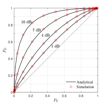
Figure 1: $P_{D}$ vs $P_{F}$ for different SNRs when $m=9,n=5$, and $p=13$.

IV ROC of the Largest Generalized Eigenvalue

Let us now analyze the behavior of detection and false alarm probabilities associated with the maximum eigenvalue based test. To this end, by exploiting the relationship between the non-zero eigenvalues of $\widehat{\boldsymbol{\Theta}}$ and $\mathbf{F}$ given by by $\hat{\lambda}_{j}=(p/n)\lambda_{j}$, for $j=1,2,\ldots,n$, we may express the c.d.f. of the maximum eigenvalue corresponding to $\widehat{\boldsymbol{\Theta}}$ as $F_{\lambda_{\max}}^{(\alpha)}(\kappa x;\gamma)$, where $\kappa=n/p$.

Now in light of Theorem 1 along with (5), (6), the detection and false alarm probabilities can be written, respectively, as

$$P_{D}(\gamma,\lambda_{\text{th}}) =1-F_{\lambda_{\max}}^{(\alpha)}(\kappa\lambda_{\text{th}};\gamma)$$ (15)

$$P_{F}(\lambda_{\text{th}}) =1-F_{\lambda_{\max}}^{(\alpha)}(\kappa\lambda_{\text{th}};0).$$ (16)

In general, obtaining an explicit functional relationship between $P_{D}$ and $P_{F}$ (i.e., the ROC profile) is an arduous task. Nevertheless, in the important case of $\alpha=0$, such an explicit relationship is possible as shown in the following corollary.

Corollary 3

In the important case of $\alpha=0$ (i.e., $p=m$), the quantities $P_{D}$ and $P_{F}$ are functionally related as

$$P_{D}=1-\frac{G^{(0)}_{\gamma}\left(\left[1-P_{F}\right]^{1/nm}\right)}{(n-1)!(1+\gamma)^{n}}.$$ (17)

Figure 2: $P_{D}$ vs $P_{F}$ for different $m$ values when $n=4$ and $p=15$.

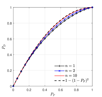
Figure 3: $P_{D}$ vs $P_{F}$ for different $n$ values when $m=100$, $p=100$ and $\gamma=m$. An upper bound on the limiting ROC profile is shown in dashed line.

Since the configuration $p=m$ barely guarantees the positive definiteness of the sample estimate of the noise-only covariance matrix[25], this represents the worst possible ROC profile.

The ROC curves corresponding to various parameter settings are shown in Figs. 1 and 2. The ROC of the maximum generalized eigenvalue is shown in Fig. 1 for different SNR values. The power improvement with the increasing SNR is clearly visible in Fig. 1. The next important parameter which affects the ROC profile is the dimensionality of the system $m$. To this end, Fig. 2 shows the effect of $m$ for fixed $n$ in two different settings: when $\gamma$ scales with $m$ (i.e., $\gamma=\theta m$) and $\gamma$ is free of $m$. As can be seen, the disparity between $m$ and $n$ degrades both ROC profiles. Since we operate below the phase transition, as $m\to p$ with $\gamma$ independent of $m$, the largest generalized eigenvalue looses its detection power, which is also visible in the figure. However, under the same setting with $\gamma=\theta m$ (i.e., $\gamma=O(m)$), the ROC profile converges to a limit as $m\to p$. To further highlight this, we depict the ROC profiles when $m=p$ and $\gamma=O(m)$ for different values of $n$ and large $m$ in Fig. 3. Although, we cannot exactly quantify this limit, our numerical results suggest a tight upper bound on this limit as $P_{D}=1-(1-P_{F})^{\theta+1}$, which is also depicted in the figure.

V Conclusion

This paper investigates the detection problem in colored noise using the largest generalized eigenvalue of whitened signal-plus-noise sample covariance matrix. In particular, our focus is on the sample deficient regime in which the number of signal-plus-noise observations is strictly less than the system dimension (i.e., $m>n$). We have assessed the performance of this detector by developing a new expression for the c.d.f. of the largest generalized eigenvalue of a complex singular $F$-matrix. It turns out that when the noise-only sample covariance matrix is nearly rank deficient (i.e., $p=m$) and $\gamma=O(m)$, the ROC profile corresponding to the largest sample generalized eigenvalue converges to a limit as $m$ increases. Since an exact evaluation of this limit seems an arduous task, we provide a tight upper bound on this limit.

Appendix A Proof of the c.d.f. of the maximum eigenvalue

We find it convenient to derive the c.d.f. of the maximum of the transformed variables $y_{j}=\lambda_{j}/(1+\lambda_{j}),\;j=1,2,\ldots,n$, since the map $y\mapsto y/(y+1)$ preserves the order. To this end, following Corollary 1, we express the joint density of $y_{1}<y_{2}<\ldots<y_{n}$ as

$$p(y_{1},\ldots,y_{n})=f\left(\frac{y_{1}}{1-y_{1}},\ldots,\frac{y_{n}}{1-y_{n}}\right)\prod_{j=1}^{n}\frac{1}{(1-y_{j})^{2}}.$$

Now by definition, the c.d.f. of $y_{\max}$ assumes the form

$$\Pr(y_{\max}\leq x)=\idotsint\limits_{0<y_{1}<\ldots<y_{n}\leq x}p(y_{1},\ldots,y_{n}){\rm d}y_{1}\ldots{\rm d}y_{n}.$$

Consequently, we exploit the symmetry and the homogeneity of each of the terms to remove the ordered region of integration and summations which in turn yields

$$\Pr(y_{\max}\leq x) =K_{\alpha}(\eta)x^{m(n-1)+1}\mathcal{A}(x)$$

$$\quad-\sum_{k=0}^{m-n-1}q_{\alpha}(\eta,k)x^{n(m-1)-k}\mathcal{B}(k,x)$$ (18)

where $K_{\alpha}(\eta)=\mathcal{K}_{2}(m,n,p)(n+\alpha)!/(n-1)!c_{\eta}^{m-1}(1+\eta)^{n}$, $q_{\alpha}(\eta,k)=\mathcal{K}_{2}(m,n,p)(m+\alpha-k-1)!/(n-1)!(1+\eta)^{n}(m-n-k-1)!c_{\eta}^{n+k}$,

$$\mathcal{A}(x)=\int_{(0,1)^{n}} \frac{(1-xy_{1})^{\alpha}}{(1-c_{\eta}xy_{1})^{n+\alpha+1}}\Delta_{n}^{2}(\mathbf{y})$$

$$\qquad\qquad\times\prod_{\ell=2}^{n}\frac{(1-xy_{\ell})^{\alpha}}{\left(y_{1}-y_{\ell}\right)}y_{\ell}^{m-n}{\rm d}\mathbf{y},$$ (19)

$$\mathcal{B}(k,x)=\int_{(0,1)^{n}} y_{1}^{m-n-k-1}(1-xy_{1})^{\alpha}\Delta_{n}^{2}(\mathbf{y})$$

$$\qquad\qquad\times\prod_{\ell=2}^{n}\frac{(1-xy_{\ell})^{\alpha}}{\left(y_{1}-y_{\ell}\right)}y_{\ell}^{m-n}{\rm d}\mathbf{y},$$ (20)

$(0,1)^{n}=(0,1)\times(0,1)\times\ldots\times(0,1)$ with $\times$ denoting the Cartesian product, and ${\rm d}\mathbf{y}={\rm d}y_{1}\ldots{\rm d}y_{n}$. Since the above two multiple integrals are structurally similar, we focus on the evaluation of $\mathcal{A}(x)$ while the other follows in a similar manner. Therefore, noting the decomposition $\Delta_{n}^{2}(\mathbf{y})=\prod_{k=2}^{n}(y_{1}-y_{k})^{2}\prod_{2\leq i<\ell\leq n}(y_{\ell}-y_{i})^{2}$, we may rewrite (A) as

$$\mathcal{A}(x)=\int_{0}^{1}\frac{(1-xy_{1})^{\alpha}}{(1-c_{\eta}xy_{1})^{n+\alpha+1}}\mathcal{Q}_{n-1}(y_{1},\beta,x){\rm d}y_{1}$$ (21)

where $\beta=m-n$ and

$$\mathcal{Q}_{n}(y_{1},\beta,x)=\int_{[0,1]^{n}}\Delta_{n}^{2}(\mathbf{z})\prod_{j=1}^{n}z_{j}^{\beta}(1-xz_{j})^{\alpha}(y_{1}-z_{j}){\rm d}\mathbf{z}.$$

The above $n$-fold integral can be evaluated with the help of [23, Ch. 22] followed by some tedious algebraic manipulation to yield

$$\mathcal{Q}_{n}(y_{1},\beta,x)$$

$$\quad=K_{(\beta,n)}x^{\alpha(n+1)}(1-xy_{1})^{-\alpha}$$

$$\qquad\quad\times\det\left[P_{n+i-1}^{(0,\beta)}\left(2y_{1}-1\right)\hskip 14.22636pt\widetilde{\Psi}_{i,j}(x)\right]_{\begin{subarray}{c}i=1,2,...,\alpha+1\\ j=2,3,...,\alpha+1\end{subarray}}$$

where $\widetilde{\Psi}_{i,j}(x)=(n+i+\beta)_{j-2}P^{(j-2,\beta+j-2)}_{n+1+i-j}\left(\frac{2}{x}-1\right)$ and

$$K_{(\beta,n)} =\prod_{j=1}^{\alpha+1}\frac{(n+j-1)!(n+\beta+j-1)!}{(2n+2j+\beta-2)!}$$

$$\qquad\qquad\times\prod_{j=0}^{n-1}\frac{j!(j+1)!(\beta+j)!}{(\beta+n+j)!}\prod_{j=0}^{\alpha-1}\frac{1}{j!}.$$

In light of the above development and noting that only the first column of the determinant depends on $y_{1}$, we rewrite (21) as

$$\mathcal{A}(x) =K_{(\beta,n-1)}x^{n\alpha}\det\left[\widetilde{\Omega}_{i}^{(\alpha)}(x,\eta)\hskip 14.22636pt\Psi_{i,j}(x)\right]_{\begin{subarray}{c}i=1,2,...,\alpha+1\\ j=2,3,...,\alpha+1\end{subarray}}$$

where $\widetilde{\Omega}_{i}^{(\alpha)}(x,\eta)=\int_{0}^{1}\frac{P_{n+i-1}^{(0,\beta)}\left(2y_{1}-1\right)}{(1-c_{\eta}xy_{1})^{n+\alpha+1}}{\rm d}y_{1}$. Now following definition 2, we may expand the denominator and perform term by term integration with the help of [26, Eq. 3.194.1] to obtain

$$\mathcal{A}(x) =\frac{K_{(\beta,n-1)}x^{n\alpha}}{(1-c_{\eta}x)^{n+p-m+1}}$$

$$\qquad\times\det\left[\Omega_{i}^{(\alpha)}(x,\eta)\hskip 14.22636pt\Psi_{i,j}(x)\right]_{\begin{subarray}{c}i=1,2,...,\alpha+1\\ j=2,3,...,\alpha+1\end{subarray}}.$$ (22)

As for $\mathcal{B}(k,x)$, following similar arguments as before, with some tedious algebraic manipulation, we obtain

$$\mathcal{B}(k,x) =(-1)^{n+1}K_{(\beta,n-1)}(\beta-k-1)!(k!)^{-1}x^{n\alpha}$$

$$\qquad\qquad\times\det\left[c_{i}(k)\hskip 14.22636pt\Psi_{i,j}(x)\right]_{\begin{subarray}{c}i=1,2,...,\alpha+1\\ j=2,3,...,\alpha+1\end{subarray}}$$ (23)

where $c_{i}(k)=(-1)^{i-1}\frac{(n+k+i-2)!}{(m+i-k-2)!}$. Finally, we substitute (A) and (A) into (A) and make use of the functional relationship $\lambda_{\max}=y_{\max}/(1-y_{\max})$ with some algebraic manipulation to conclude the proof.

References

• [1] R. R. Nadakuditi and A. Edelman, “Sample eigenvalue based detection of high-dimensional signals in white noise using relatively few samples,” IEEE Trans. Signal Process., vol. 56, no. 7, pp. 2625–2638, Jul. 2008.
• [2] R. R. Nadakuditi and J. W. Silverstein, “Fundamental limit of sample generalized eigenvalue based detection of signals in noise using relatively few signal-bearing and noise-only samples,” IEEE J. Sel. Topics Signal Process., vol. 4, no. 3, pp. 468–480, Jun. 2010.
• [3] A. Onatski, “Detection of weak signals in high-dimensional complex-valued data,” Random Matrices: Theory and Applications, vol. 03, no. 01, p. 1450001, 2014.
• [4] L. D. Chamain, P. Dharmawansa, S. Atapattu, and C. Tellambura, “Eigenvalue-based detection of a signal in colored noise: Finite and asymptotic analyses,” IEEE Trans. Inf. Theory, vol. 66, no. 10, pp. 6413–6433, 2020.
• [5] I. M. Johnstone and B. Nadler, “Roy’s largest root test under rank-one alternatives,” Biometrika, vol. 104, no. 1, pp. 181–193, 2017.
• [6] P. Dharmawansa, B. Nadler, and O. Shwartz, “Roy‘s largest root under rank-one perturbations: The complex valued case and applications,” J. Multivar. Anal., vol. 174, p. 104524, 2019.
• [7] P. Dharmawansa, I. M. Johnstone, and A. Onatski, “Local asymptotic normality of the spectrum of high-dimensional spiked F-ratios,” arXiv:1411.3875 [math.ST], Nov. 2014.
• [8] Q. Wang and J. Yao, “Extreme eigenvalues of large-dimensional spiked Fisher matrices with application,” Ann. Statist., vol. 45, no. 1, pp. 415–460, Feb. 2017.
• [9] J. Baik, G. B. Arous, and S. Péché, “Phase transition of the largest eigenvalue for non-null complex sample covariance matrices,” Ann. Probab., vol. 33, no. 5, pp. 1643–1697, 2005.
• [10] J. Baik and J. W. Silverstein, “Eigenvalues of large sample covariance matrices of spiked population models,” J. Multivariate Anal., vol. 97, no. 6, pp. 1382–1408, 2006.
• [11] R. Couillet and M. Debbah, Random Matrix Methods for Wireless Communications.   Cambridge University Press, Sep. 2011.
• [12] E. Maris, “A resampling method for estimating the signal subspace of spatio-temporal EEG/MEG data,” IEEE Trans. Biomed. Eng., vol. 50, no. 8, pp. 935–949, Aug 2003.
• [13] J. Vinogradova, R. Couillet, and W. Hachem, “Statistical inference in large antenna arrays under unknown noise pattern,” IEEE Trans. Signal Process., vol. 61, no. 22, pp. 5633–5645, Nov. 2013.
• [14] S. Hiltunen, P. Loubaton, and P. Chevalier, “Large system analysis of a GLRT for detection with large sensor arrays in temporally white noise,” IEEE Trans. Signal Process., vol. 63, no. 20, pp. 5409–5423, Oct. 2015.
• [15] N. Asendorf and R. R. Nadakuditi, “Improved detection of correlated signals in low-rank-plus-noise type data sets using informative canonical correlation analysis (ICCA),” IEEE Trans. Inf. Theory, vol. 63, no. 6, pp. 3451–3467, Jun. 2017.
• [16] M. S. Srivastava, “Singular wishart and multivariate beta distributions,” Ann. Stat., vol. 31, no. 5, pp. 1537–1560, 2003.
• [17] R. K. Mallik, “The pseudo-wishart distribution and its application to MIMO systems,” IEEE Trans. Inf. Theory, vol. 49, no. 10, pp. 2761–2769, 2003.
• [18] H. Uhlig, “On singular wishart and singular multivariate beta distributions,” Ann. Stat., pp. 395–405, 1994.
• [19] T. Ratnarajah and R. Vaillancourt, “Complex singular wishart matrices and applications,” Comput. Math. with Appl., vol. 50, no. 3-4, pp. 399–411, 2005.
• [20] A. Onatski, “The tracy-widom limit for the largest eigenvalues of singular complex wishart matrices,” Ann. Appl. Probab., vol. 18, no. 2, pp. 470–490, 2008.
• [21] K. Shimizu and H. Hashiguchi, “Expressing the largest eigenvalue of a singular beta f-matrix with heterogeneous hypergeometric functions,” Random Matrices: Theory Appl., vol. 11, no. 01, p. 2250005, 2022.
• [22] D. Wang, “The largest eigenvalue of real symmetric, Hermitian and Hermitian self-dual random matrix models with rank one external source, part I,” J. Stat. Phys., vol. 146, no. 4, pp. 719–761, 2012.
• [23] M. L. Mehta, Random Matrices.   Academic Press, 2004, vol. 142.
• [24] L. C. Andrews, Special Functions of Mathematics for Engineers.   SPIE Press, 1998.
• [25] R. J. Muirhead, Aspects of Multivariate Statistical Theory.   John Wiley & Sons, 2009, vol. 197.
• [26] I. Gradshteyn and I. Ryzhik, Table of Integrals, Series, and Products, 7th ed.   Boston: Academic Press, 2007.