Efficient and reliable divergence-conforming methods for an elasticity-poroelasticity interface problem

Abstract.

We present a finite element discretisation to model the interaction between a poroelastic structure and an elastic medium. The consolidation problem considers fully coupled deformations across an interface, ensuring continuity of displacement and total traction, as well as no-flux for the fluid phase. Our formulation of the poroelasticity equations incorporates displacement, fluid pressure, and total pressure, while the elasticity equations adopt a displacement-pressure formulation. Notably, the transmission conditions at the interface are enforced without the need for Lagrange multipliers. We demonstrate the stability and convergence of the divergence-conforming finite element method across various polynomial degrees. The a priori error bounds remain robust, even when considering large variations in intricate model parameters such as Lamé constants, permeability, and storativity coefficient. To enhance computational efficiency and reliability, we develop residual-based a posteriori error estimators that are independent of the aforementioned coefficients. Additionally, we devise parameter-robust and optimal block diagonal preconditioners. Through numerical examples, including adaptive scenarios, we illustrate the scheme’s properties such as convergence and parameter robustness.

Keywords. Biot–elasticity transmission equations, mixed finite element methods, divergence-conforming schemes, a priori error analysis, a posteriori error analysis, operator preconditioning.

1. Introduction

In a variety of engineering and biomedical applications, poroelastic bodies are either surrounded or in contact with a purely elastic material. Examples include filter design, prosthetics, simulation of oil extraction from reservoirs, carbon sequestration, and sound insulation structures. From the viewpoint of constructing and analysing numerical methods, recent works for the interfacial Biot/elasticity problem can be found in [5, 4, 25, 26, 27]. These contributions include mortar-type discretisations, formulations using rotations, and extensions to lubrication models. In this work we focus on H(div)-conforming discretisations of displacement for the transmission problem, in combination with a total pressure formulation for both the elastic and poroelastic sub-domains. Divergence-conforming methods with tangential jump penalisation for elasticity were already proposed in [32]. Their counterpart for Biot poroelasticity equations (in the two-field formulation) have been introduced in [34, 47, 48], while a much more abundant literature is available for Brinkman flows (as well as coupled flow-transport problems) in [16, 17, 30, 35]. The extension to interfacial porous media flow has been addressed in [18, 19, 24, 33]. In general, such type of discretisations offer appealing features such as local conservation of mass, and the ability to produce robust and locking–free schemes. These type of schemes are required because of the large number of parameters upon which robustness is targeted (especially in the limits of near incompressibility and near impermeability).

As regularity of the solution is not always available (due to possibly high contrast in material parameters, domain singularities, etc), we are also interested in deriving a posteriori error estimates which allow us to apply adaptive mesh refinement in the regions where it is most required. A coupled elliptic–parabolic a posteriori error analysis for Biot poroelasticity and multiple network poroelasticity is available from the works [1, 22, 38]. On the other hand, robust estimates for the elasticity–poroelasticity coupling have been obtained only recently, for enriched Galerkin methods in [26], and in [4] for rotation-based formulations.

Here the analysis is carried out considering two examples of fluid pressure approximation: either continuous or discontinuous piecewise polynomials. For the DG case we use a classical symmetric interior penalty (SIP) method. In all cases the proposed formulation is robust with respect to material parameters that can assume very small or very large values, including the extreme cases of near incompressibility, near impermeability, and near zero storativity. This parameter independence in the stability of the discrete problem is critical in the a priori error bounds, in the derivation of a posteriori error estimates, and in the design of robust preconditioners.

Finally, we design optimal preconditioner that are robust with respect to parameters. The preconditioner is block-diagonal and its definition relies on the stability properties of the proposed numerical scheme, i.e., it consists in a discretisation of the continuous Riesz map (see [37, 30] for similar approaches). The definition of the pressure block is motivated by [42], where a robust preconditioner for the interface Stokes problems with high contrast is proposed.

The remainder of the paper has been structured as follows. Section 2 is devoted to the description of the interfacial problem, it states boundary and transmission conditions, and there we give the continuous weak formulation. The discrete problem in two different formulations is defined in Section 3. The stability and solvability of the H(div)-conforming methods is addressed in Section 4. Residual-based a posteriori error estimators are constructed and analysed in Section 5. The operator framework and definition of a norm-equivalent preconditioner is addressed in Section 6, and numerical methods that confirm the properties of the proposed methods are collected in Section 7.

2. Problem statement

2.1. Preliminaries

Standard notation on Lebesgue and Sobolev spaces together with their associated norms will be adopted throughout the presentation. For $s\geq 0$ and a generic domain $\mathcal{D}$, the symbol $\mathrm{H}^{s}(\mathcal{D})$ denotes the usual Sobolev space equipped with the norm $\|\cdot\|_{s,\mathcal{D}}$ and seminorm $|\cdot|_{s,\mathcal{D}}$. The case $s=0$ is understood as the space $\mathrm{L}^{2}(\mathcal{D})$. Boldfaces will be used to denote vector-valued spaces, maintaining the same notation as scalar spaces for the norms and seminorms. For a Banach space $V$, we will use the symbol $V^{\prime}$ to denote its dual space. We also recall the definition of the space $\mathbf{H}(\mathop{\mathrm{div}}\nolimits,\mathcal{D}):=\{\bm{v}\in\mathbf{L}^{2}(\mathcal{D}):\mathop{\mathrm{div}}\nolimits\bm{v}\in\mathrm{L}^{2}(\mathcal{D})\}$, which is of Hilbert type when endowed with the norm $\|\bm{v}\|^{2}_{\mathop{\mathrm{div}}\nolimits,\mathcal{D}}=\|\bm{v}\|^{2}_{0,\mathcal{D}}+\|\mathop{\mathrm{div}}\nolimits\bm{v}\|^{2}_{0,\mathcal{D}}$. As usual, throughout the paper the notation $A\lesssim B$ will abbreviate the inequality $A\leq CB$ where $C$ is a generic constant that does not depend on the maximal mesh sizes $h$ nor on the sensitive parameters of the model, in particular the Lamé parameters on each subdomain (and will proceed similarly for $A\gtrsim B$). The constants in the inequalities will be specified whenever necessary from the context.

2.2. The transmission problem

Following the problem setup from [25, 26], let us consider a bounded Lipschitz domain $\Omega\subset\mathbb{R}^{d}$, $d\in\{2,3\}$, together with a partition into non-overlapping and connected subdomains $\Omega^{\mathrm{E}}$, $\Omega^{\mathrm{P}}$ representing zones occupied by an elastic body (e.g., a non-pay rock, in the context of reservoir modelling) and a fluid-saturated poroelastic region (e.g., a reservoir), respectively. The interface between the two subdomains is denoted as $\Sigma=\partial\Omega^{\mathrm{P}}\cap\partial\Omega^{\mathrm{E}}$, and on it the normal vector $\bm{n}$ is assumed to point from $\Omega^{\mathrm{P}}$ to $\Omega^{\mathrm{E}}$. The boundary of the domain $\Omega$ is separated in terms of the boundaries of two individual subdomains, that is $\partial\Omega:=\Gamma^{\mathrm{P}}\cup\Gamma^{\mathrm{E}}$, and then subdivided as the disjoint Dirichlet and Neumann type condition as $\Gamma^{\mathrm{P}}:=\Gamma^{\mathrm{P}}_{D}\cup\Gamma^{\mathrm{P}}_{N}$ and $\Gamma^{\mathrm{E}}:=\Gamma^{\mathrm{E}}_{D}\cup\Gamma^{\mathrm{E}}_{N}$, respectively. We assume that all sub-boundaries have positive $(d-1)$–Hausdorff measure.

In the overall domain we state the momentum balance of the fluid and solid phases on the poroelastic region, the mass conservation of the total amount of fluid, and the balance of linear momentum on the elastic region. In doing so, and following [5], in addition to the usual variables of elastic displacement, poroelastic displacement, and fluid pressure, we employ the total pressure in the poroelastic subdomain, and the Herrmann pressure in the elastic subdomain. For given body loads $\bm{b}^{\mathrm{P}}(t):\Omega^{\mathrm{P}}\to\mathbb{R}^{d}$, $\bm{b}^{\mathrm{E}}(t):\Omega^{\mathrm{E}}\to\mathbb{R}^{d}$, and a volumetric source or sink $\ell^{\mathrm{P}}(t):\Omega^{\mathrm{P}}\to\mathbb{R}$, one seeks for each time $t\in(0,t_{\mathrm{final}}]$, the vector of solid displacements $\bm{u}^{\mathrm{E}}:\Omega^{\mathrm{E}}\to\mathbb{R}^{d}$ of the non-pay zone, the elastic pressure $\varphi^{\mathrm{E}}:\Omega^{\mathrm{E}}\to\mathbb{R}$, the displacement $\bm{u}^{\mathrm{P}}(t):\Omega^{\mathrm{P}}\to\mathbb{R}^{d}$, the pore fluid pressure $p^{\mathrm{P}}(t):\Omega^{\mathrm{P}}\to\mathbb{R}$, and the total pressure $\varphi^{\mathrm{P}}(t):\Omega^{\mathrm{P}}\to\mathbb{R}$ of the reservoir, satisfying:

$$-\mathop{\mathbf{div}}\nolimits(2{\mu^{\mathrm{P}}}\bm{\varepsilon}(\bm{u}^{\mathrm{P}})-\varphi^{\mathrm{P}}\mathbf{I}) =\bm{b}^{\mathrm{P}} \text{in $\Omega^{\mathrm{P}}\times(0,t_{\mathrm{final}}]$},$$ (2.1a)

$$\biggl{(}c_{0}+\frac{\alpha^{2}}{{\lambda^{\mathrm{P}}}}\biggr{)}\partial_{t}p^{\mathrm{P}}-\frac{\alpha}{{\lambda^{\mathrm{P}}}}\partial_{t}\varphi^{\mathrm{P}}-\frac{1}{\eta}\mathop{\mathrm{div}}\nolimits(\kappa\nabla p^{\mathrm{P}}) =\ell^{\mathrm{P}} \text{in $\Omega^{\mathrm{P}}\times(0,t_{\mathrm{final}}]$},$$ (2.1b)

$$\varphi^{\mathrm{P}}-\alpha p^{\mathrm{P}}+{\lambda^{\mathrm{P}}}\mathop{\mathrm{div}}\nolimits\bm{u}^{\mathrm{P}} =0 \text{in $\Omega^{\mathrm{P}}\times(0,t_{\mathrm{final}}]$},$$ (2.1c)

$$-\mathop{\mathbf{div}}\nolimits(2{\mu^{\mathrm{E}}}\bm{\varepsilon}(\bm{u}^{\mathrm{E}})-\varphi^{\mathrm{E}}\mathbf{I}) =\bm{b}^{\mathrm{E}} \text{in $\Omega^{\mathrm{E}}\times(0,t_{\mathrm{final}}]$},$$ (2.1d)

$$\varphi^{\mathrm{E}}+{\lambda^{\mathrm{E}}}\mathop{\mathrm{div}}\nolimits\bm{u}^{\mathrm{E}} =0 \text{in $\Omega^{\mathrm{E}}\times(0,t_{\mathrm{final}}]$}.$$ (2.1e)

Here $\kappa(\bm{x})$ is the hydraulic conductivity of the porous medium, $\eta$ is the constant viscosity of the interstitial fluid, $c_{0}$ is the storativity coefficient, $\alpha$ is the Biot–Willis consolidation parameter, and $\mu^{\mathrm{E}},\lambda^{\mathrm{E}}$ and $\mu^{\mathrm{P}},\lambda^{\mathrm{P}}$ are the Lamé parameters associated with the constitutive law of the solid on the elastic and on the poroelastic subdomain, respectively. The poroelastic stress $\widetilde{\bm{\sigma}}=\bm{\sigma}-\alpha p^{\mathrm{P}}\mathbf{I}$ is composed by the effective mechanical stress ${\lambda^{\mathrm{P}}}(\mathop{\mathrm{div}}\nolimits\bm{u}^{\mathrm{P}})\mathbf{I}+2{\mu^{\mathrm{P}}}\bm{\varepsilon}(\bm{u}^{\mathrm{P}})$ plus the non-viscous fluid stress (the fluid pressure scaled with $\alpha$). This system is complemented by the following set of boundary conditions

$$\bm{u}^{\mathrm{P}}=\bm{0}\quad\text{and}\quad\frac{\kappa}{\eta}\nabla p^{\mathrm{P}}\cdot\bm{n}^{\Gamma}=0 \text{on $\Gamma^{\mathrm{P}}_{D}\times(0,t_{\mathrm{final}}]$},$$ (2.2a)

$$[2{\mu^{\mathrm{P}}}\bm{\varepsilon}(\bm{u}^{\mathrm{P}})-\varphi^{\mathrm{P}}\mathbf{I}]\bm{n}^{\Gamma}=\bm{0}\quad\text{and}\quad p^{\mathrm{P}}=0 \text{on $\Gamma^{\mathrm{P}}_{N}\times(0,t_{\mathrm{final}}]$},$$ (2.2b)

$$\bm{u}^{\mathrm{E}}=\bm{0} \text{on $\Gamma^{\mathrm{E}}_{D}\times(0,t_{\mathrm{final}}]$},$$ (2.2c)

$$[2{\mu^{\mathrm{E}}}\bm{\varepsilon}(\bm{u}^{\mathrm{E}})-\varphi^{\mathrm{E}}\mathbf{I}]\bm{n}^{\Gamma}=\bm{0} \text{on $\Gamma^{\mathrm{E}}_{N}\times(0,t_{\mathrm{final}}]$}.$$ (2.2d)

Here, the partition $\Gamma^{\mathrm{P}}:=\Gamma^{\mathrm{P}}_{D}\cup\Gamma^{\mathrm{P}}_{N}$ denotes the sub-boundaries where we impose essential (i.e., $\bm{u}^{\mathrm{P}}=\bm{0}$) and natural boundary conditions (i.e., $\widetilde{\bm{\sigma}}\bm{n}^{\Gamma}=\bm{0}$) corresponding to equation (2.1a). For ease of notation, we note that, in this definition, we are assuming that the essential and natural sub-boundaries corresponding to equation (2.1b) (i.e., the ones where we impose $p^{\mathrm{P}}=0$ and $\nabla p^{\mathrm{P}}\cdot\bm{n}^{\Gamma}=0$, respectively) match the natural and essential sub-boundaries associated to (2.1a), respectively. However, in general, this does not have to be case, and one may choose separately the partition into essential and natural for each of these two equations separately.

Along with the previous set of boundary conditions, the system is also complemented by transmission conditions in the absence of external forces (derived by means of homogenisation in [41]) that take the following form

$$\bm{u}^{\mathrm{P}}=\bm{u}^{\mathrm{E}},\quad[2{\mu^{\mathrm{P}}}\bm{\varepsilon}(\bm{u}^{\mathrm{P}})-\varphi^{\mathrm{P}}\mathbf{I}]\bm{n}=[2{\mu^{\mathrm{E}}}\bm{\varepsilon}(\bm{u}^{\mathrm{E}})-\varphi^{\mathrm{E}}\mathbf{I}]\bm{n},\quad\frac{\kappa}{\eta}\nabla p^{\mathrm{P}}\cdot\bm{n}=0\quad\text{on $\Sigma\times(0,t_{\mathrm{final}}]$},$$ (2.3)

which represent continuity of the medium, the balance of total tractions, and no-flux of fluid at the interface, respectively. An advantage with respect to [5] is that here we can use the full poroelastic stresses to impose the transmission conditions. We also consider the following initial conditions

$$p^{\mathrm{P}}(0)=0,\quad\bm{u}^{\mathrm{P}}(0)=\bm{0}\qquad\qquad\text{in $\Omega^{\mathrm{P}}$}.$$

Homogeneity of the boundary and initial conditions is only assumed to simplify the exposition of the subsequent analysis, however the results remain valid for more general assumptions. We also note that non-homogeneous boundary conditions are used in the numerical experiments.

2.3. A weak formulation

As the paper focuses on the spatial discretisation, we will restrict the problem formulation to the steady case. For this, we define the function spaces

$$\mathbf{V}^{\mathrm{E}}:=\mathbf{H}^{1}_{\Gamma_{D}^{\mathrm{E}}}(\Omega^{\mathrm{E}}),\quad\mathbf{V}^{\mathrm{P}}:=\mathbf{H}^{1}_{\Gamma_{D}^{\mathrm{P}}}(\Omega^{\mathrm{P}}),\quad\mathrm{Q}^{\mathrm{P}}:=\mathrm{H}^{1}_{\Gamma_{N}^{\mathrm{P}}}(\Omega^{\mathrm{P}}),\quad\mathrm{Z}^{\mathrm{E}}:=\mathrm{L}^{2}(\Omega^{\mathrm{E}}),\quad\mathrm{Z}^{\mathrm{P}}:=\mathrm{L}^{2}(\Omega^{\mathrm{P}}).$$

Considering a backward Euler discretisation in time with constant time step $\Delta t$, multiplying the time-discrete version of (2.1b) by adequate test functions, integrating by parts (in space) whenever appropriate, and using the boundary conditions (2.2c)-(2.2d), leads to the following weak formulation: Find $\bm{u}^{\mathrm{P}}\in\mathbf{V}^{\mathrm{P}},\bm{u}^{\mathrm{E}}\in\mathbf{V}^{\mathrm{E}},p^{\mathrm{P}}\in\mathrm{Q}^{\mathrm{P}},\varphi^{\mathrm{E}}\in\mathrm{Z}^{\mathrm{E}},\varphi^{\mathrm{P}}(t)\in\mathrm{Z}^{\mathrm{P}}$ such that

$$2{\mu^{\mathrm{P}}}(\bm{\varepsilon}(\bm{u}^{\mathrm{P}}),\bm{\varepsilon}(\bm{v}^{\mathrm{P}}))_{0,\Omega^{\mathrm{P}}}-(\varphi^{\mathrm{P}},\mathop{\mathrm{div}}\nolimits\bm{v}^{\mathrm{P}})_{0,\Omega^{\mathrm{P}}}-\langle[2{\mu^{\mathrm{P}}}\bm{\varepsilon}(\bm{u}^{\mathrm{P}})-\varphi^{\mathrm{P}}\mathbf{I}]\bm{n},\bm{v}^{\mathrm{P}}\rangle_{{\Gamma^{P}_{D}}} =(\bm{b}^{\mathrm{P}},\bm{v}^{\mathrm{P}})_{0,\Omega^{\mathrm{P}}},$$

$$(\varphi^{\mathrm{P}},\psi^{\mathrm{P}})_{0,\Omega^{\mathrm{P}}}-\alpha(p^{\mathrm{P}},\psi^{\mathrm{P}})_{0,\Omega^{\mathrm{P}}}+{\lambda^{\mathrm{P}}}(\psi^{\mathrm{P}},\mathop{\mathrm{div}}\nolimits\bm{u}^{\mathrm{P}})_{0,\Omega^{\mathrm{P}}} =0,$$

$$\frac{1}{\Delta t}\biggl{(}c_{0}+\frac{\alpha^{2}}{{\lambda^{\mathrm{P}}}}\biggr{)}(p^{\mathrm{P}},q^{\mathrm{P}})_{0,\Omega^{\mathrm{P}}}-\frac{1}{\Delta t}\frac{\alpha}{{\lambda^{\mathrm{P}}}}(\varphi^{\mathrm{P}},q^{\mathrm{P}})_{0,\Omega^{\mathrm{P}}}+\frac{1}{\eta}(\kappa\nabla p^{\mathrm{P}},\nabla q^{\mathrm{P}})_{0,\Omega^{\mathrm{P}}}-\frac{1}{\eta}\langle\kappa\nabla p^{\mathrm{P}}\cdot\bm{n},q^{\mathrm{P}}\rangle_{\partial\Omega^{\mathrm{P}}} =(\ell^{\mathrm{P}},q^{\mathrm{P}})_{0,\Omega^{\mathrm{P}}},$$

$$2{\mu^{\mathrm{E}}}(\bm{\varepsilon}(\bm{u}^{\mathrm{E}}),\bm{\varepsilon}(\bm{v}^{\mathrm{E}}))_{0,\Omega^{\mathrm{E}}}-(\varphi^{\mathrm{E}},\mathop{\mathrm{div}}\nolimits\bm{v}^{\mathrm{E}})_{0,\Omega^{\mathrm{E}}}-\langle[2{\mu^{\mathrm{E}}}\bm{\varepsilon}(\bm{u}^{\mathrm{E}})-\varphi^{\mathrm{E}}\mathbf{I}]\bm{n}^{\partial\Omega^{\mathrm{E}}},\bm{v}^{\mathrm{E}}\rangle_{{\Gamma_{D}^{E}}} =(\bm{b}^{\mathrm{E}},\bm{v}^{\mathrm{E}})_{0,\Omega^{\mathrm{E}}},$$

$$(\varphi^{\mathrm{E}},\psi^{\mathrm{E}})_{0,\Omega^{\mathrm{E}}}+{\lambda^{\mathrm{E}}}(\psi^{\mathrm{E}},\mathop{\mathrm{div}}\nolimits\bm{u}^{\mathrm{E}})_{0,\Omega^{\mathrm{E}}} =0.$$

Note that we can simply define a global displacement $\bm{u}\in\mathbf{V}:=\mathbf{H}^{1}_{\Gamma_{D}}(\Omega)$ (through continuity of the medium in (2.3)) such that $\bm{u}|_{\Omega^{\mathrm{P}}}=\bm{u}^{\mathrm{P}}$ and $\bm{u}|_{\Omega^{\mathrm{E}}}=\bm{u}^{\mathrm{E}}$; as well as a global pressure (it is the total pressure on the poroelastic medium and the elastic hydrostatic pressure on the elastic subdomain) $\varphi\in\mathrm{Z}:=\mathrm{L}^{2}(\Omega)$ such that $\varphi|_{\Omega^{\mathrm{P}}}=\varphi^{\mathrm{P}}$ and $\varphi|_{\Omega^{\mathrm{E}}}=\varphi^{\mathrm{E}}$. Similarly, we define the body load $\bm{b}\in\mathbf{L}^{2}(\Omega)$ composed by $\bm{b}|_{\Omega^{\mathrm{P}}}=\bm{b}^{\mathrm{P}}$ and $\bm{b}|_{\Omega^{\mathrm{E}}}=\bm{b}^{\mathrm{E}}$, and also the global Lamé parameters $\mu$ and $\lambda$ as $\mu|_{\Omega^{\mathrm{P}}}=\mu^{\mathrm{P}},\,\lambda|_{\Omega^{\mathrm{P}}}=\lambda^{\mathrm{P}}$ and $\mu|_{\Omega^{\mathrm{E}}}=\mu^{\mathrm{E}},\,\lambda|_{\Omega^{\mathrm{E}}}=\lambda^{\mathrm{E}}$. We also multiply the weak form of the mass conservation equation by -1. The steps above in combination with the second and third transmission conditions in (2.3), yield: Find $\bm{u}\in\mathbf{V},\,p^{\mathrm{P}}\in\mathrm{Q}^{\mathrm{P}},\,\varphi\in\mathrm{Z}$ such that

$$a_{1}(\bm{u},\bm{v}) \;+ \;b_{1}(\bm{v},\varphi) = \;F(\bm{v}) \quad\forall\bm{v}\in\mathbf{V},$$ (2.4a)

$${-}\tilde{a}_{2}\biggl{(}\frac{1}{\Delta t}p^{\mathrm{P}},q^{\mathrm{P}}\biggr{)} \;{-} a_{2}(p^{\mathrm{P}},q^{\mathrm{P}}) \;{+} \;b_{2}\biggl{(}q^{\mathrm{P}},\,\frac{1}{\Delta t}\varphi\biggr{)} = \;G(q^{\mathrm{P}}) \quad\forall q^{\mathrm{P}}\in\mathrm{Q}^{\mathrm{P}},$$ (2.4b)

$$b_{1}(\bm{u},\psi) \;+\; b_{2}(p^{\mathrm{P}},\psi) \;- \;a_{3}(\varphi,\psi) = 0 \quad\forall\psi\in\mathrm{Z},$$ (2.4c)

where the bilinear forms $a_{1}:\mathbf{V}\times\mathbf{V}\to\mathbb{R}$, $a_{2}:Q^{\mathrm{P}}\times\mathrm{Q}^{\mathrm{P}}\to\mathbb{R}$, $a_{3}:\mathrm{Z}\times\mathrm{Z}\to\mathbb{R}$, $b_{1}:\mathbf{V}\times\mathrm{Z}\to\mathbb{R}$, $b_{2}:Q^{\mathrm{P}}\times\mathrm{Z}\to\mathbb{R}$, and linear functionals $F:\mathbf{V}\to\mathbb{R}$, $G:Q^{\mathrm{P}}\to\mathbb{R}$, adopt the following form

$$a_{1}(\bm{u},\bm{v}):=2(\mu\,\bm{\varepsilon}(\bm{u}),\bm{\varepsilon}(\bm{v}))_{0,\Omega},\qquad b_{1}(\bm{v},\psi):=-(\psi,\mathop{\mathrm{div}}\nolimits\bm{v})_{0,\Omega},\qquad F(\bm{v}):=(\bm{b},\bm{v})_{0,\Omega},$$

$$\tilde{a}_{2}(p^{\mathrm{P}},q^{\mathrm{P}}):=\biggl{(}c_{0}+\frac{\alpha^{2}}{{\lambda^{\mathrm{P}}}}\biggr{)}(p^{\mathrm{P}},q^{\mathrm{P}})_{0,\Omega^{\mathrm{P}}},\qquad a_{2}(p^{\mathrm{P}},q^{\mathrm{P}}):=\frac{1}{\eta}(\kappa\nabla p^{\mathrm{P}},\nabla q^{\mathrm{P}})_{0,\Omega^{\mathrm{P}}},$$ (2.5)

$$b_{2}(p^{\mathrm{P}},\psi):=\frac{\alpha}{{\lambda^{\mathrm{P}}}}(p^{\mathrm{P}},\psi^{\mathrm{P}})_{0,\Omega^{\mathrm{P}}},\qquad a_{3}(\varphi,\psi):=(\frac{1}{\lambda}\varphi,\psi)_{0,\Omega},\qquad G(q^{\mathrm{P}}):={-}(\ell^{\mathrm{P}},q^{\mathrm{P}})_{0,\Omega^{\mathrm{P}}}.$$

2.4. Properties of the continuous weak form and further assumptions

The variational forms above satisfy the continuity bounds

$$a_{1}(\bm{u},\bm{v})\leq\|\sqrt{2\mu}\bm{\varepsilon}(\bm{u})\|_{0,\Omega}\|\sqrt{2\mu}\bm{\varepsilon}(\bm{v})\|_{0,\Omega}\lesssim\|\sqrt{2\mu}\bm{u}\|_{1,\Omega}\|\sqrt{2\mu}\bm{v}\|_{1,\Omega},$$

$$b_{1}(\bm{v},\psi)\leq\|\mathop{\mathrm{div}}\nolimits\bm{v}\|_{0,\Omega}\|\psi\|_{0,\Omega}\lesssim\|\sqrt{2\mu}\bm{v}\|_{1,\Omega}\|\frac{1}{\sqrt{2\mu}}\psi\|_{0,\Omega},$$

$$a_{2}(p^{\mathrm{P}},q^{\mathrm{P}})\leq\|\sqrt{\frac{\kappa}{\eta}}\nabla p^{\mathrm{P}}\|_{0,\Omega^{\mathrm{P}}}\|\sqrt{\frac{\kappa}{\eta}}\nabla q^{\mathrm{P}}\|_{0,\Omega^{\mathrm{P}}},\qquad a_{3}(\varphi,\psi)\leq\|\frac{1}{\sqrt{\lambda}}\varphi\|_{0,\Omega}\|\frac{1}{\sqrt{\lambda}}\psi\|_{0,\Omega},$$

$$b_{2}(q^{\mathrm{P}},\psi)\leq\|\frac{\alpha}{\sqrt{\lambda^{\mathrm{P}}}}q^{\mathrm{P}}\|_{0,\Omega^{\mathrm{P}}}\|\frac{1}{\sqrt{\lambda^{\mathrm{P}}}}\psi^{\mathrm{P}}\|_{0,\Omega^{\mathrm{P}}},\qquad F(\bm{v})\lesssim\|\bm{b}\|_{0,\Omega}\|\bm{v}\|_{1,\Omega},\qquad G(q^{\mathrm{P}})\leq\|\ell^{\mathrm{P}}\|_{0,\Omega^{\mathrm{P}}}\|q^{\mathrm{P}}\|_{0,\Omega^{\mathrm{P}}},$$

for all $\bm{u},\bm{v}\in\mathbf{V}$, $\psi,\varphi\in\mathrm{Z}$, $p^{\mathrm{P}},q^{\mathrm{P}}\in\mathrm{Q}^{\mathrm{P}}$. There also holds coercivity of the diagonal bilinear forms

$$a_{1}(\bm{v},\bm{v})\geq\|\sqrt{2\mu}\bm{\varepsilon}(\bm{v})\|_{0,\Omega}^{2}\gtrsim\|\sqrt{2\mu}\bm{v}\|_{1,\Omega}^{2},\quad{|a_{2}(q^{\mathrm{P}},q^{\mathrm{P}})|}\geq\|\sqrt{\frac{\kappa}{\eta}}\nabla q^{\mathrm{P}}\|_{0,\Omega^{\mathrm{P}}}^{2},\quad a_{3}(\psi,\psi)\geq\|\frac{1}{\sqrt{\lambda}}\psi\|_{0,\Omega}^{2},$$

for all $\bm{v}\in\mathbf{V}$, $q^{\mathrm{P}}\in\mathrm{Q}^{\mathrm{P}}$, $\psi\in\mathrm{Z}$, and the following inf-sup condition (see, e.g., [23]): There exists $\xi>0$ such that

$$\sup_{\bm{v}(\neq\bm{0})\in\mathbf{V}}\frac{b_{1}(\bm{v},\psi)}{\|\bm{v}\|_{1,\Omega}}\geq\xi\|\psi\|_{0,\Omega}\qquad\forall\psi\in\mathrm{Z}.$$ (2.6)

Details on the unique solvability of the continuous problem can be found in [25, 27], or, for the steady case with rotation-based formulations, in [5, 4] (but in those references the analysis assumes that the pay-zone poroelastic subdomain is completely confined by the elastic structure).

Similarly to the relevant inf-sup condition (2.6), we have that for each $\varphi_{0}\in\mathrm{L}^{2}(\Omega)$ with $\varphi_{0}|_{\Omega^{\mathrm{E}}}=\varphi_{0}^{\mathrm{E}}\in\mathrm{L}^{2}(\Omega^{\mathrm{E}})$ and $\varphi_{0}|_{\Omega^{\mathrm{P}}}=\varphi_{0}^{\mathrm{P}}\in\mathrm{L}^{2}(\Omega^{\mathrm{P}})$, we can find $\bm{v}_{0}^{\mathrm{E}}\in\mathbf{H}^{1}_{\Gamma_{D}^{\mathrm{E}},0}(\Omega^{\mathrm{E}})$ and $\bm{v}_{0}^{\mathrm{P}}\in\mathbf{H}^{1}_{\Gamma_{D}^{\mathrm{P}},0}(\Omega^{\mathrm{P}})$, where $\mathbf{H}^{1}_{\Gamma_{D}^{\mathrm{E}},0}(\Omega^{\mathrm{E}})=\{\bm{v}:\bm{v}\in\mathbf{H}^{1}_{\Gamma_{D}^{\mathrm{E}}}(\Omega^{\mathrm{E}})\;\mbox{and}\;\bm{v}|_{\Sigma}=\bm{0}\}$ and $\mathbf{H}^{1}_{\Gamma_{D}^{\mathrm{P}},0}(\Omega^{\mathrm{P}})=\{\bm{v}:\bm{v}\in\mathbf{H}^{1}_{\Gamma_{D}^{\mathrm{P}}}(\Omega^{\mathrm{P}})\;\mbox{and}\;\bm{v}|_{\Sigma}=\bm{0}\}$, such that

$$(\mathop{\mathrm{div}}\nolimits\bm{v}_{0}^{\mathrm{E}},\varphi^{\mathrm{E}}_{0})_{0,\Omega^{\mathrm{E}}}\geq C_{\Omega^{\mathrm{E}}}/\mu^{\mathrm{E}}\|\varphi^{\mathrm{E}}_{0}\|_{0,\Omega^{\mathrm{E}}}^{2},\quad\sqrt{2\mu^{\mathrm{E}}}\|\bm{\nabla}\bm{v}_{0}^{\mathrm{E}}\|_{0,\Omega^{\mathrm{E}}}\leq 1/\sqrt{2\mu^{\mathrm{E}}}\|\varphi^{\mathrm{E}}_{0}\|_{0,\Omega^{\mathrm{E}}},$$

$$(\mathop{\mathrm{div}}\nolimits\bm{v}_{0}^{\mathrm{P}},\varphi^{\mathrm{P}}_{0})_{0,\Omega^{\mathrm{P}}}\geq C_{\Omega^{\mathrm{P}}}/\mu^{\mathrm{P}}\|\varphi^{\mathrm{P}}_{0}\|_{0,\Omega^{\mathrm{P}}}^{2},\quad\sqrt{2\mu^{\mathrm{P}}}\|\bm{\nabla}\bm{v}_{0}^{\mathrm{P}}\|_{0,\Omega^{\mathrm{P}}}\leq 1/\sqrt{2\mu^{\mathrm{P}}}\|\varphi^{\mathrm{P}}_{0}\|_{0,\Omega^{\mathrm{P}}}.$$

Hence, there exists $\bm{v}_{0}\in\mathbf{V}$ such that $\bm{v}_{0}|_{\Omega^{\mathrm{E}}}=\bm{v}_{0}^{\mathrm{E}}$ and $\bm{v}_{0}|_{\Omega^{\mathrm{P}}}=\bm{v}_{0}^{\mathrm{P}}$. Moreover we have

$$\sup_{\bm{0}\neq\bm{v}\in\mathbf{V}}\frac{b_{1}(\bm{v},\varphi_{0})}{\|\sqrt{2\mu}\bm{v}\|_{1,\Omega}}\geq\tilde{C}\|\frac{1}{\sqrt{2\mu}}\varphi_{0}\|_{0,\Omega},$$

or, following also [42], we can write

$$\sup_{\bm{0}\neq\bm{v}\in\mathbf{V}}\frac{b_{1}(\bm{v},\varphi_{0})}{\|\sqrt{2\mu}\bm{\varepsilon}(\bm{v})\|_{0,\Omega}}\geq\tilde{C}\|\frac{1}{\sqrt{2\mu}}\varphi_{0}\|_{0,\Omega},$$

for a positive constant $\tilde{C}$ independent of $\mu$.

3. An H(div)-conforming finite element approximation

We denote by $\{{\mathcal{T}}_{h}^{\mathrm{P}}\}_{h}$ and $\{{\mathcal{T}}_{h}^{\mathrm{E}}\}_{h}$ sequences of triangular (or tetrahedral in 3D) partitions of the poroelastic and elastic subdomains $\Omega^{\mathrm{P}}$ and $\Omega^{\mathrm{E}}$, respectively having diameter $h_{K}$, and being such that the partitions are conforming with the interface $\Sigma$. We label by $K^{-}$ and $K^{+}$ the two elements adjacent to a facet (an edge in 2D or a face in 3D), while $h_{e}$ stands for the maximum diameter of the facet. By $\mathcal{E}_{h}$ we will denote the set of all facets and will distinguish between facets lying on the elastic, poroelastic, and interfacial regions $\mathcal{E}_{h}=\mathcal{E}_{h}^{\mathrm{E}}\cup\mathcal{E}_{h}^{\mathrm{P}}\cup\mathcal{E}_{h}^{\Sigma}$.

For a smooth vector, scalar, or tensor field $w$ defined on $\mathcal{T}_{h}$, $w^{\pm}$ denote its traces taken from the interior of $K^{+}$ and $K^{-}$, respectively. We also denote by $\bm{n}^{\pm}$ the outward unit normal vector to $K^{\pm}$. The symbols ${\left\{\kern-3.01385pt\left\{\cdot\right\}\kern-3.01385pt\right\}}$ and $\llbracket\cdot\rrbracket$ denote, respectively, the average and jump operators, defined as

$${\left\{\kern-3.01385pt\left\{w\right\}\kern-3.01385pt\right\}}\coloneqq\frac{1}{2}(w^{-}+w^{+}),\quad\llbracket w\odot\bm{n}\rrbracket\coloneqq(w^{-}\odot\bm{n}^{-}+w^{+}\odot\bm{n}^{+}),$$ (3.1)

for a generic multiplication operator $\odot$, which applies to interior edges, whereas for boundary jumps and averages we adopt the conventions ${\left\{\kern-3.01385pt\left\{w\right\}\kern-3.01385pt\right\}}=w$, and $\llbracket w\odot\bm{n}\rrbracket=w\odot\bm{n}$. The element-wise action of a differential operator is denoted with a subindex $h$, for example, $\nabla_{h}$, $\bm{\nabla}_{h}$ will denote the broken gradient operators for scalar and vector quantities, respectively and $\bm{\varepsilon}_{h}(\cdot)=\frac{1}{2}(\bm{\nabla}_{h}\cdot+(\bm{\nabla}_{h}\cdot)^{T})$ is the symmetrised vector broken gradient.

Let $\mathbb{P}_{k}(K)$ denote the local space spanned by polynomials of degree up to $k\geq 0$, and let us consider the following discrete spaces

$$\begin{split}\mathbf{V}_{h}&\coloneqq\bigl{\{}\bm{v}_{h}\in\mathbf{H}(\mathop{\mathrm{div}}\nolimits;\Omega):\bm{v}_{h}|_{K}\in[\mathbb{P}_{k+1}(K)]^{d}\quad\forall K\in\mathcal{T}_{h},\quad\bm{v}_{h}\cdot\bm{n}|_{\Gamma_{D}^{\mathrm{E}}\cup\Gamma_{D}^{\mathrm{P}}}=0\bigr{\}},\\ \mathrm{Q}^{\mathrm{P}}_{h}&\coloneqq\bigl{\{}q^{\mathrm{P}}_{h}\in\mathrm{Q}^{\mathrm{P}}:q_{h}|_{K}\in\mathbb{P}_{k+1}(K)\quad\forall K\in\mathcal{T}_{h}^{\mathrm{P}}\bigr{\}},\\ \mathrm{Z}_{h}&\coloneqq\bigl{\{}\psi_{h}\in\mathrm{Z}:\psi_{h}|_{K}\in\mathbb{P}_{k}(K)\quad\forall K\in\mathcal{T}_{h}\bigr{\}},\end{split}$$ (3.2)

which, in particular, satisfy the so-called equilibrium property

$$\mathop{\mathrm{div}}\nolimits\mathbf{V}_{h}=\mathrm{Z}_{h}.$$ (3.3)

Note that in this case $\mathbf{V}_{h}$ is the space of divergence-conforming BDM elements [15], and it is not conforming with $\mathbf{V}$. Its basic approximation property, locally on $K\in\mathcal{T}_{h}$, is that for all $\bm{v}\in\mathbf{H}^{s}(K)$, there exists an interpolant $\bm{v}_{I}\in\mathbf{V}_{h}(K)$ such that

$$\|\bm{v}-\bm{v}_{I}\|_{0,K}+h_{K}|\bm{v}-\bm{v}_{I}|_{1,K}+h_{K}^{2}|\bm{v}-\bm{v}_{I}|_{2,K}\lesssim h_{K}^{s}|\bm{v}|_{s,K},\qquad 2\leq s\leq k,$$ (3.4)

see, e.g., [15, 17, 35].

3.1. Formulation with continuous fluid pressure

The Galerkin finite element formulation then reads: Find $(\bm{u}_{h},p^{\mathrm{P}}_{h},\varphi_{h})\in\mathbf{V}_{h}\times\mathrm{Q}^{\mathrm{P}}_{h}\times\mathrm{Z}_{h}$ such that:

$$a_{1}^{h}(\bm{u}_{h},\bm{v}_{h}) \;+ \;{b}_{1}(\bm{v}_{h},\varphi_{h}) = \;F(\bm{v}_{h}) \quad\forall\bm{v}_{h}\in\mathbf{V}_{h},$$ (3.5a)

$${-}\tilde{a}_{2}(p_{h}^{\mathrm{P}},q_{h}^{\mathrm{P}}) \;{-} a_{2}(p_{h}^{\mathrm{P}},q_{h}^{\mathrm{P}}) \;{+} \;b_{2}(q_{h}^{\mathrm{P}},\,\varphi_{h}) = \;G(q_{h}^{\mathrm{P}}) \quad\forall q_{h}^{\mathrm{P}}\in\mathrm{Q}_{h}^{\mathrm{P}},$$ (3.5b)

$${b}_{1}(\bm{u}_{h},\psi_{h}) \;+\; b_{2}(p_{h}^{\mathrm{P}},\psi_{h}) \;- \;a_{3}(\varphi_{h},\psi_{h}) = 0 \quad\forall\psi_{h}\in\mathrm{Z}_{h},$$ (3.5c)

where $a_{1}^{h}(\cdot,\cdot)$ is the discrete version of the bilinear form $a_{1}(\cdot,\cdot)$ and it is defined using a symmetric interior penalty from [35] (see also [33] for its use in the context of poroelasticity)

$$a^{h}_{1}(\bm{u}_{h},\bm{v}_{h}) \coloneqq 2(\mu\bm{\varepsilon}_{h}(\bm{u}_{h}),\bm{\varepsilon}_{h}(\bm{v}_{h}))_{0,\Omega}-2\sum_{e\in\mathcal{E}_{h}{\cup\Gamma_{D}^{*}}}\bigl{(}\langle{\left\{\kern-3.01385pt\left\{\mu\bm{\varepsilon}_{h}(\bm{u}_{h})\right\}\kern-3.01385pt\right\}},\llbracket\bm{v}_{h}\otimes\bm{n}\rrbracket\rangle_{0,e}+\langle{\left\{\kern-3.01385pt\left\{\mu\bm{\varepsilon}_{h}(\bm{v}_{h})\right\}\kern-3.01385pt\right\}},\llbracket\bm{u}_{h}\otimes\bm{n}\rrbracket\rangle_{0,e}\bigr{)}$$

$$\quad+2\sum_{e\in\mathcal{E}_{h}{\cup\Gamma_{D}^{*}}\setminus\mathcal{E}_{h}^{\Sigma}}\frac{\beta_{\bm{u}}}{h_{e}}\langle\mu\llbracket\bm{u}_{h}\otimes\bm{n}\rrbracket,\llbracket\bm{v}_{h}\otimes\bm{n}\rrbracket\rangle_{0,e}+2\sum_{e\in\mathcal{E}_{h}^{\Sigma}}\frac{\beta_{\bm{u}}}{h_{e}}\langle\mu^{0}\llbracket\bm{u}_{h}\otimes\bm{n}\rrbracket,\llbracket\bm{v}_{h}\otimes\bm{n}\rrbracket\rangle_{0,e},$$ (3.6)

where $\Gamma_{D}^{*}=\Gamma_{D}^{\mathrm{P}}\cup\Gamma_{D}^{\mathrm{E}}$ denotes the part of the boundary where Dirichlet conditions are imposed on displacement, $\beta_{\bm{u}}>0$ is a parameter penalising the (tangential) displacement jumps (and also serving as a Nitsche parameter to enforce the tangential part of the displacement boundary condition) so that the bilinear form $a^{h}_{1}(\cdot,\cdot)$ is positive definite, and $\mu^{0}=\max\{\mu^{\mathrm{E}},\mu^{\mathrm{P}}\}$. Now we write down the above weak formulation (3.5) in the following compact form: Find $(\bm{u}_{h},p^{\mathrm{P}}_{h},\varphi_{h})\in\mathbf{V}_{h}\times\mathrm{Q}^{\mathrm{P}}_{h}\times\mathrm{Z}_{h}$ such that

$$M_{h}(\bm{u}_{h},p^{\mathrm{P}}_{h},\varphi_{h};\bm{v}_{h},q^{\mathrm{P}}_{h},\psi_{h}) =F(\bm{v}_{h})+G(q_{h}^{\mathrm{P}})\quad\forall(\bm{v}_{h},q^{\mathrm{P}}_{h},\psi_{h})\in\mathbf{V}_{h}\times\mathrm{Q}^{\mathrm{P}}_{h}\times\mathrm{Z}_{h},$$

where the multilinear form is defined as

$$M_{h}(\bm{u}_{h},p^{\mathrm{P}}_{h},\varphi_{h};\bm{v}_{h},q^{\mathrm{P}}_{h},\psi_{h}) =a_{1}^{h}(\bm{u}_{h},\bm{v}_{h})+{b}_{1}(\bm{v}_{h},\varphi_{h}){-}\tilde{a}_{2}(p_{h}^{\mathrm{P}},q_{h}^{\mathrm{P}}){-}a_{2}(p_{h}^{\mathrm{P}},q_{h}^{\mathrm{P}})$$

$$\qquad+b_{2}(q_{h}^{\mathrm{P}},\,\varphi_{h})+{b}_{1}(\bm{u}_{h},\psi_{h})+b_{2}(p_{h}^{\mathrm{P}},\psi_{h})-a_{3}(\varphi_{h},\psi_{h}).$$

Continuity and coercivity also hold for the modified bilinear form $a_{1}^{h}(\cdot,\cdot)$, but they do over the discrete space $\mathbf{V}_{h}$ and with respect to the following mesh-dependent and parameter-dependent broken norms

$$\left\|\bm{v}_{h}\right\|_{*,\mathcal{T}_{h}}^{2} \coloneqq\sum_{K\in\mathcal{T}_{h}}\left\|\sqrt{2\mu}\bm{\varepsilon}_{h}(\bm{v}_{h})\right\|_{0,K}^{2}+\sum_{e\in\mathcal{E}_{h}\cup\Gamma_{D}^{*}\setminus\mathcal{E}_{h}^{\Sigma}}2{\mu}\frac{\beta_{\bm{u}}}{h_{e}}\left\|\llbracket\bm{v}_{h}\otimes\bm{n}\rrbracket\right\|_{0,e}^{2}+\sum_{e\in\mathcal{E}_{h}^{\Sigma}}2{\mu_{0}}\frac{\beta_{\bm{u}}}{h_{e}}\left\|\llbracket\bm{v}_{h}\otimes\bm{n}\rrbracket\right\|_{0,e}^{2},$$

$$\left\|\bm{v}_{h}\right\|_{1,\mathcal{T}_{h}}^{2} \coloneqq\left\|\sqrt{2\mu}\bm{v}_{h}\right\|_{0,\Omega}^{2}+\left\|\bm{v}_{h}\right\|_{*,\mathcal{T}_{h}}^{2}\ \text{for all $\bm{v}_{h}\in\mathbf{H}^{1}(\mathcal{T}_{h})$,}$$ (3.7)

$$\left\|\bm{v}_{h}\right\|_{2,\mathcal{T}_{h}}^{2} \coloneqq\left\|\bm{v}_{h}\right\|_{1,\mathcal{T}_{h}}^{2}+\sum_{K\in\mathcal{T}_{h}}h_{K}^{2}|\sqrt{2\mu}\bm{v}|_{2,K}^{2}\ \text{for all $\bm{v}_{h}\in\mathbf{H}^{2}(\mathcal{T}_{h})$,}$$

where, for a generic $s\geq 0$, the broken vectorial Sobolev spaces are defined as

$$\mathbf{H}^{s}(\mathcal{T}_{h})\coloneqq\bigl{\{}\bm{v}_{h}\in\mathbf{L}^{2}(\Omega):\bm{v}_{h}|_{K}\in\mathbf{H}^{s}(K),\ K\in\mathcal{T}_{h}\bigr{\}}.$$

Thanks to the discrete version of Korn’s inequality [14, eq. (1.12)], the norms above are uniformly equivalent over the appropriate spaces. Similarly, for the present choice of finite element spaces, a discrete inf-sup condition for $b_{1}(\cdot,\cdot)$ holds naturally in the discrete norm $\left\|\cdot\right\|_{1,\mathcal{T}_{h}}$ when we do not have a weighting with the space-dependent parameter $\mu$ (cf. [35]). However, combined with the arguments in Section 2.4, we can assert that there exists $\hat{\xi}>0$, independent of $h$ and of $\mu$, such that

$$\sup_{\bm{v}_{h}(\neq\bm{0})\in\mathbf{V}_{h}}\frac{b_{1}(\bm{v}_{h},\psi_{h})}{\|\bm{v}_{h}\|_{1,\mathcal{T}_{h}}}\geq\hat{\xi}\|\frac{1}{\sqrt{2\mu}}\psi_{h}\|_{0,\Omega}\qquad\forall\psi_{h}\in\mathrm{Z}_{h}.$$

3.2. Formulation with discontinuous fluid pressure

Consider now the spaces

$$\begin{split}\mathbf{V}_{h}\coloneqq\bigl{\{}\bm{v}_{h}\in\mathbf{H}(\mathop{\mathrm{div}}\nolimits;\Omega):\bm{v}_{h}|_{K}\in[\mathbb{P}_{k+1}(K)]^{d}\quad\forall K\in\mathcal{T}_{h},\quad\bm{v}_{h}\cdot\bm{n}|_{\Gamma_{D}^{\mathrm{E}}\cup\Gamma_{D}^{\mathrm{P}}}=0\bigr{\}},\\ \widetilde{\mathrm{Q}}^{\mathrm{P}}_{h}\coloneqq\bigl{\{}q^{\mathrm{P}}_{h}\in\mathrm{L}^{2}(\Omega^{\mathrm{P}}):q_{h}|_{K}\in\mathbb{P}_{k+1}(K)\quad\forall K\in\mathcal{T}_{h}^{\mathrm{P}}\bigr{\}},\qquad\mathrm{Z}_{h}\coloneqq\bigl{\{}\psi_{h}\in\mathrm{Z}:\psi_{h}|_{K}\in\mathbb{P}_{k}(K)\quad\forall K\in\mathcal{T}_{h}\bigr{\}}.\end{split}$$ (3.8)

The formulation in this case reads: Find $(\bm{u}_{h},p^{\mathrm{P}}_{h},\varphi_{h})\in\mathbf{V}_{h}\times\widetilde{\mathrm{Q}}^{\mathrm{P}}_{h}\times\mathrm{Z}_{h}$ such that:

$$a_{1}^{h}(\bm{u}_{h},\bm{v}_{h}) \;+ \;{b}_{1}(\bm{v}_{h},\varphi_{h}) = \;F(\bm{v}_{h}) \quad\forall\bm{v}_{h}\in\mathbf{V}_{h},$$ (3.9a)

$${-}\tilde{a}_{2}(p_{h}^{\mathrm{P}},q_{h}^{\mathrm{P}}) \;{-} a_{2}^{h}(p_{h}^{\mathrm{P}},q_{h}^{\mathrm{P}}) \;{+} \;b_{2}(q_{h}^{\mathrm{P}},\,\varphi_{h}) = \;G(q_{h}^{\mathrm{P}}) \quad\forall q_{h}^{\mathrm{P}}\in\widetilde{\mathrm{Q}}_{h}^{\mathrm{P}},$$ (3.9b)

$${b}_{1}(\bm{u}_{h},\psi_{h}) \;+\; b_{2}(p_{h}^{\mathrm{P}},\psi_{h}) \;- \;a_{3}(\varphi_{h},\psi_{h}) = 0 \quad\forall\psi_{h}\in\mathrm{Z}_{h},$$ (3.9c)

where $a_{2}^{h}(\cdot,\cdot)$ is the discrete version of the bilinear form $a_{2}(\cdot,\cdot)$ and it is defined using a symmetric interior penalty from, e.g., the classical paper [6]

$$a^{h}_{2}(p_{h}^{\mathrm{P}},q_{h}^{\mathrm{P}}) \coloneqq\biggl{(}\frac{\kappa}{\eta}\nabla_{h}p_{h}^{\mathrm{P}},\nabla_{h}q_{h}^{\mathrm{P}}\biggr{)}_{0,\Omega}-\sum_{e\in\mathcal{E}_{h}^{\mathrm{P}}{\cup\Gamma_{D}^{\mathrm{P}}}}\biggl{(}\biggl{\langle}{\left\{\kern-3.01385pt\left\{\frac{\kappa}{\eta}\nabla_{h}p_{h}^{\mathrm{P}}\right\}\kern-3.01385pt\right\}},\llbracket q_{h}^{\mathrm{P}}\bm{n}\rrbracket\biggr{\rangle}_{0,e}+\biggl{\langle}{\left\{\kern-3.01385pt\left\{\frac{\kappa}{\eta}\nabla_{h}q_{h}^{\mathrm{P}}\right\}\kern-3.01385pt\right\}},\llbracket p_{h}^{\mathrm{P}}\bm{n}\rrbracket\biggr{\rangle}_{0,e}\biggr{)}$$

$$\quad+\sum_{e\in\mathcal{E}_{h}^{\mathrm{P}}{\cup\Gamma_{D}^{\mathrm{P}}}}\frac{\beta_{p^{\mathrm{P}}}}{h_{e}}\biggl{\langle}\frac{\kappa}{\eta}\llbracket p_{h}^{\mathrm{P}}\bm{n}\rrbracket,\llbracket q_{h}^{\mathrm{P}}\bm{n}\rrbracket\biggr{\rangle}_{0,e},$$ (3.10)

where $\beta_{p^{\mathrm{P}}}>0$ is a parameter penalising the pressure jumps. If $\beta_{p^{\mathrm{P}}}$ is sufficiently large, this yields the coercivity of the bilinear form $a^{h}_{2}$.

Next, and as done for the case of continuous pressure approximation, we write down the compact form of the above weak formulation (3.9): Find $(\bm{u}_{h},p^{\mathrm{P}}_{h},\varphi_{h})\in\mathbf{V}_{h}\times\widetilde{\mathrm{Q}}^{\mathrm{P}}_{h}\times\mathrm{Z}_{h}$ such that

$$\widetilde{M}_{h}(\bm{u}_{h},p^{\mathrm{P}}_{h},\varphi_{h};\bm{v}_{h},q^{\mathrm{P}}_{h},\psi_{h}) =F(\bm{v}_{h})+G(q_{h}^{\mathrm{P}})\quad\forall(\bm{v}_{h},q^{\mathrm{P}}_{h},\psi_{h})\in\mathbf{V}_{h}\times\widetilde{\mathrm{Q}}^{\mathrm{P}}_{h}\times\mathrm{Z}_{h},$$

where

$$\widetilde{M}_{h}(\bm{u}_{h},p^{\mathrm{P}}_{h},\varphi_{h};\bm{v}_{h},q^{\mathrm{P}}_{h},\psi_{h}) =a_{1}^{h}(\bm{u}_{h},\bm{v}_{h})+{b}_{1}(\bm{v}_{h},\varphi_{h}){-}\tilde{a}_{2}(p_{h}^{\mathrm{P}},q_{h}^{\mathrm{P}}){-}a_{2}^{h}(p_{h}^{\mathrm{P}},q_{h}^{\mathrm{P}})$$

$$\qquad+b_{2}(q_{h}^{\mathrm{P}},\,\varphi_{h})+{b}_{1}(\bm{u}_{h},\psi_{h})+b_{2}(p_{h}^{\mathrm{P}},\psi_{h})-a_{3}(\varphi_{h},\psi_{h}).$$

4. Unique solvability of the discrete problems and a priori error estimates

4.1. Well-posedness analysis for formulation (3.5)

We proceed by means of a Fortin argument and consider the canonical interpolation operator $\Pi_{h}:\mathbf{V}\rightarrow\mathbf{V}_{h}$ such that

$$b_{1}(\bm{v}-\Pi_{h}\bm{v},\varphi_{h}) =0\qquad\forall\varphi_{h}\in\mathrm{Z}_{h},$$ (4.1a)

$$|\bm{v}-\Pi_{h}\bm{v}|_{s,K} \leq Ch^{t-s}|\bm{v}|_{t,K}\quad\forall K\in\mathcal{T}_{h},$$ (4.1b)

where $C$ is a positive constant which depends only on the shape of $K$ and $1\leq t\leq r+1$ (see, e.g., [13]).

Using the trace inequality and property (4.1b), we have the following bound in one of the norms from (3.1)

$$\|\bm{v}-\Pi_{h}\bm{v}\|_{\ast,\mathcal{T}_{h}}\leq\|\bm{v}\|_{\ast,\mathcal{T}_{h}}\quad\forall\bm{v}\in\mathbf{V}.$$

Moreover, we have

$$\|\Pi_{h}\bm{v}\|_{\ast,\mathcal{T}_{h}}\leq C\|\bm{v}\|_{\ast,\mathcal{T}_{h}}.$$

With these properties satisfied by the operator $\Pi_{h}$, we can use the continuous inf-sup condition to readily show that there exists $\xi>0$ such that a discrete inf-sup condition for the bilinear form $b_{1}$:

$$\sup_{\bm{v}\in\mathbf{V}_{h}\setminus\{\bm{0}\}}\frac{b_{1}(\bm{v},\varphi_{h})}{\|\bm{v}\|_{\ast,\mathcal{T}_{h}}}\geq\sup_{\Pi_{h}\bm{v}\in\mathbf{V}_{h}\setminus\{\bm{0}\}}\frac{b_{1}(\Pi_{h}\bm{v},\varphi_{h})}{\|\Pi_{h}\bm{v}\|_{\ast,\mathcal{T}_{h}}}=\sup_{\bm{v}\in\mathbf{V}\setminus\{\bm{0}\}}\frac{b_{1}(\bm{v},\varphi_{h})}{\|\Pi_{h}\bm{v}\|_{\ast,\mathcal{T}_{h}}}\geq\frac{1}{C}\sup_{\bm{v}\in\mathbf{V}\setminus\{\bm{0}\}}\frac{b_{1}(\bm{v},\varphi_{h})}{\|\bm{v}\|_{\ast,\mathcal{T}_{h}}}\geq\xi\|\frac{1}{\sqrt{2\mu}}\varphi_{h}\|_{0,\Omega}\quad\forall\varphi_{h}\in\mathrm{Z}_{h}.$$

We are now in a position to establish a global inf-sup condition.

Theorem 4.1.

For every $(\bm{u}_{h},p^{\mathrm{P}}_{h},\varphi_{h})\in\mathbf{V}_{h}\times\mathrm{Q}^{\mathrm{P}}_{h}\times\mathrm{Z}_{h}$, there exists $(\bm{v}_{h},q^{\mathrm{P}}_{h},\psi_{h})\in\mathbf{V}_{h}\times\mathrm{Q}^{\mathrm{P}}_{h}\times\mathrm{Z}_{h}$ with $\VERT(\bm{v}_{h},q^{\mathrm{P}}_{h},\psi_{h})\VERT\lesssim\VERT(\bm{u}_{h},p^{\mathrm{P}}_{h},\varphi_{h})\VERT$ such that

$$M_{h}(\bm{u}_{h},p^{\mathrm{P}}_{h},\varphi_{h};\bm{v}_{h},q^{\mathrm{P}}_{h},\psi_{h})\gtrsim\VERT(\bm{u}_{h},p^{\mathrm{P}}_{h},\varphi_{h})\VERT^{2},$$

where

$$\VERT(\bm{v}_{h},q^{\mathrm{P}}_{h},\psi_{h})\VERT^{2}:=\left\|\bm{v}_{h}\right\|_{*,\mathcal{T}_{h}}^{2}+\|\frac{1}{\sqrt{2\mu}}\psi_{h}\|^{2}_{0,\Omega}+\frac{1}{\lambda^{\mathrm{E}}}\|\psi_{h}\|^{2}_{0,\Omega^{\mathrm{E}}}+\frac{1}{\lambda^{\mathrm{P}}}\|\psi_{h}-\alpha q^{\mathrm{P}}_{h}\|^{2}_{0,\Omega^{\mathrm{P}}}+c_{0}\|q^{\mathrm{P}}_{h}\|^{2}_{0,\Omega^{\mathrm{P}}}+\|\frac{\kappa}{\eta}\nabla q^{\mathrm{P}}_{h}\|^{2}_{0,\Omega^{\mathrm{P}}}.$$ (4.2)

Moreover, we have that

$$\bigl{|}M_{h}(\bm{u}_{h},p^{\mathrm{P}}_{h},\varphi_{h};\bm{v}_{h},q^{\mathrm{P}}_{h},\psi_{h})\bigr{|}\lesssim\VERT(\bm{u}_{h},p^{\mathrm{P}}_{h},\varphi_{h})\VERT\VERT(\bm{v}_{h},q^{\mathrm{P}}_{h},\psi_{h})\VERT,$$

for all $(\bm{u}_{h},p^{\mathrm{P}}_{h},\varphi_{h}),(\bm{v}_{h},q^{\mathrm{P}}_{h},\psi_{h})\in\mathbf{V}_{h}\times\mathrm{Q}^{\mathrm{P}}_{h}\times\mathrm{Z}_{h}$.

Proof. Let $(\bm{u}_{h},p^{\mathrm{P}}_{h},\varphi_{h})\in\mathbf{V}_{h}\times\mathrm{Q}^{\mathrm{P}}_{h}\times\mathrm{Z}_{h}$ be arbitrary. Using the definition of the multilinear form $M_{h}$, we easily obtain

$$M_{h}(\bm{u}_{h},p^{\mathrm{P}}_{h},\varphi_{h};\bm{v}_{h},0,0)=a_{1}^{h}(\bm{u}_{h},\bm{v}_{h})+{b}_{1}(\bm{v}_{h},\varphi_{h})\geq\left(\xi-\frac{1}{2\epsilon_{1}}\right)\|\frac{1}{\sqrt{2\mu}}\varphi_{h}\|_{0,\Omega}^{2}-\frac{\epsilon_{1}}{2}\|\bm{u}_{h}\|_{\ast,\mathcal{T}_{h}}.$$

Selecting $\bm{v}=\bm{u}_{h}$, $q^{\mathrm{P}}=-p_{h}^{\mathrm{P}}$ and $\psi=-\varphi_{h}$ we have

$$M_{h}(\bm{u}_{h},p^{\mathrm{P}}_{h},\varphi_{h},\bm{u}_{h},{-}p^{\mathrm{P}}_{h},-\varphi_{h}) =a_{1}^{h}(\bm{u}_{h},\bm{u}_{h})+{\tilde{a}_{2}(p_{h}^{\mathrm{P}},p_{h}^{\mathrm{P}})}+a_{2}(p_{h}^{\mathrm{P}},p_{h}^{\mathrm{P}})-2b_{2}(p_{h}^{\mathrm{P}},\,\varphi_{h})+a_{3}(\varphi_{h},\varphi_{h})$$

$$\geq C_{2}\|\bm{u}_{h}\|_{\ast,\mathcal{T}_{h}}^{2}+c_{0}\|p_{h}^{\mathrm{P}}\|_{0,\Omega^{\mathrm{P}}}^{2}+1/\lambda^{\mathrm{E}}\|\varphi_{h}\|^{2}_{0,\Omega^{\mathrm{E}}}+1/\lambda^{\mathrm{P}}\|\varphi_{h}-\alpha p^{\mathrm{P}}_{h}\|^{2}_{0,\Omega^{\mathrm{P}}}$$

$$\qquad+c_{0}\|p^{\mathrm{P}}_{h}\|^{2}_{0,\Omega^{\mathrm{P}}}+\|\kappa/\eta\nabla p^{\mathrm{P}}_{h}\|^{2}_{0,\Omega^{\mathrm{P}}}.$$

Then we can make the choice $\bm{v}=\bm{u}_{h}+\delta_{1}\bm{v}_{h}$, $q^{\mathrm{P}}=-p_{h}^{\mathrm{P}}$ and $\psi=-\varphi_{h}$, leading to

$$M_{h}(\bm{u}_{h},p^{\mathrm{P}}_{h},\varphi_{h},\bm{u}_{h}+\delta_{1}\bm{v}_{h},-p^{\mathrm{P}}_{h},-\varphi_{h})$$

$$=M_{h}(\bm{u}_{h},p^{\mathrm{P}}_{h},\varphi_{h},\bm{u}_{h},-p^{\mathrm{P}}_{h},-\varphi_{h})+\delta_{1}M_{h}(\bm{u}_{h},p^{\mathrm{P}}_{h},\varphi_{h},\bm{v}_{h},0,0)$$

$$\geq C_{2}\|\bm{u}_{h}\|_{\ast,\mathcal{T}_{h}}^{2}+c_{0}\|p_{h}^{\mathrm{P}}\|_{0,\Omega^{\mathrm{P}}}^{2}+1/\lambda^{\mathrm{E}}\|\varphi_{h}\|^{2}_{0,\Omega^{\mathrm{E}}}+1/\lambda^{\mathrm{P}}\|\varphi_{h}-\alpha p^{\mathrm{P}}_{h}\|^{2}_{0,\Omega^{\mathrm{P}}}$$

$$\qquad+c_{0}\|p^{\mathrm{P}}_{h}\|^{2}_{0,\Omega^{\mathrm{P}}}+\|\kappa/\eta(\nabla p^{\mathrm{P}}_{h})\|^{2}_{0,\Omega^{\mathrm{P}}}+\delta_{1}\left(\xi-\frac{1}{2\epsilon_{1}}\right)\|\frac{1}{\sqrt{2\mu}}\varphi_{h}\|_{0,\Omega}^{2}-\delta_{1}\frac{\epsilon_{1}}{2}\|\bm{u}_{h}\|_{\ast,\mathcal{T}_{h}}$$

$$\geq\left(C_{2}-\delta_{1}\frac{\epsilon_{1}}{2}\right)\|\bm{u}_{h}\|_{\ast,\mathcal{T}_{h}}^{2}+c_{0}\|p_{h}^{\mathrm{P}}\|_{0,\Omega^{\mathrm{P}}}^{2}+1/\lambda^{\mathrm{E}}\|\varphi_{h}\|^{2}_{0,\Omega^{\mathrm{E}}}+1/\lambda^{\mathrm{P}}\|\varphi_{h}-\alpha p^{\mathrm{P}}_{h}\|^{2}_{0,\Omega^{\mathrm{P}}}$$

$$\qquad+c_{0}\|p^{\mathrm{P}}_{h}\|^{2}_{0,\Omega^{\mathrm{P}}}+\|\kappa/\eta(\nabla p^{\mathrm{P}}_{h})\|^{2}_{0,\Omega^{\mathrm{P}}}+\delta_{1}\left(\xi-\frac{1}{2\epsilon_{1}}\right)\|\frac{1}{\sqrt{2\mu}}\varphi_{h}\|_{0,\Omega}^{2},$$

where we have used Young’s inequality. Assuming the values $\epsilon_{1}=1/\xi$ and $\delta_{1}=C_{2}/\epsilon_{1}$, we then have

$$M_{h}(\bm{u}_{h},p^{\mathrm{P}}_{h},\varphi_{h};\bm{v}_{h},q^{\mathrm{P}}_{h},\psi_{h})\geq\frac{1}{2}\min\left\{C_{2}\xi^{2},C_{2}\right\}\VERT(\bm{u}_{h},p^{\mathrm{P}}_{h},\varphi_{h})\VERT^{2},$$

and the first part of the proof concludes after realising that

$$\VERT(\bm{v}_{h},q^{\mathrm{P}}_{h},\psi_{h})\VERT^{2}=\VERT(\bm{u}_{h}+\delta_{1}\bm{v},-p^{\mathrm{P}}_{h},-\varphi_{h})\VERT^{2}\leq 2\VERT(\bm{u}_{h},p^{\mathrm{P}}_{h},\varphi_{h})\VERT^{2}.$$

For the continuity property, it suffices to apply Cauchy–Schwarz inequality and the definition of $M_{h}$. $\square$

Lemma 4.1.

Let $(\tilde{\bm{u}},\tilde{p}^{\mathrm{P}},\tilde{\varphi})$ be a generic triplet in $\mathbf{V}_{h}\times\mathrm{Q}^{\mathrm{P}}_{h}\times\mathrm{Z}_{h}$. Then the following estimate holds

$$\VERT(\bm{u}-\bm{u}_{h},p-p^{\mathrm{P}}_{h},\varphi-\varphi_{h})\VERT\lesssim\VERT(\bm{u}-\tilde{\bm{u}},p^{\mathrm{P}}-\tilde{p}^{\mathrm{P}},\varphi-\tilde{\varphi})\VERT+\biggl{(}\sum_{K\in\mathcal{T}_{h}}h_{K}^{2}|\sqrt{2\mu}(\bm{u}-\tilde{\bm{u}})|_{2,K}^{2}\biggr{)}^{1/2}.$$

Proof. Directly from triangle inequality we have

$$\VERT(\bm{u}-\bm{u}_{h},p-p^{\mathrm{P}}_{h},\varphi-\varphi_{h})\VERT\leq\VERT(\bm{u}-\tilde{\bm{u}},p^{\mathrm{P}}-\tilde{p}^{\mathrm{P}},\varphi-\tilde{\varphi})\VERT+\VERT(\tilde{\bm{u}}-\bm{u}_{h},\tilde{p}^{\mathrm{P}}-p^{\mathrm{P}}_{h},\tilde{\varphi}-\varphi_{h})\VERT.$$

Using Theorem 4.1 and the properties of $M_{h}$ gives

$$\VERT(\tilde{\bm{u}}-\bm{u}_{h},\tilde{p}^{\mathrm{P}}-p^{\mathrm{P}}_{h},\tilde{\varphi}-\varphi_{h})\VERT^{2} \lesssim M_{h}(\tilde{\bm{u}}-\bm{u}_{h},\tilde{p}^{\mathrm{P}}-p^{\mathrm{P}}_{h},\tilde{\varphi}-\varphi_{h};\bm{v}_{h},q^{\mathrm{P}}_{h},\psi_{h})$$

$$\leq M_{h}(\tilde{\bm{u}},\tilde{p}^{\mathrm{P}},\tilde{\varphi};\bm{v}_{h},q^{\mathrm{P}}_{h},\psi_{h})-M_{h}(\bm{u}_{h},p^{\mathrm{P}}_{h},\varphi_{h};\bm{v}_{h},q^{\mathrm{P}}_{h},\psi_{h})$$

$$\leq M_{h}(\tilde{\bm{u}}-\bm{u},\tilde{p}^{\mathrm{P}}-p^{\mathrm{P}},\tilde{\varphi}-\varphi;\bm{v}_{h},q^{\mathrm{P}}_{h},\psi_{h})$$

$$\lesssim\VERT(\bm{u}-\tilde{\bm{u}},p^{\mathrm{P}}-\tilde{p}^{\mathrm{P}},\varphi-\tilde{\varphi})\VERT$$

$$\qquad\qquad+\biggl{(}\sum_{K\in\mathcal{T}_{h}}h_{K}^{2}|\sqrt{2\mu}(\bm{u}-\tilde{\bm{u}})|_{2,K}^{2}\biggr{)}^{1/2}\VERT(\tilde{\bm{u}}-\bm{u}_{h},\tilde{p}^{\mathrm{P}}-p^{\mathrm{P}}_{h},\tilde{\varphi}-\varphi_{h})\VERT.$$

$\square$

4.2. Well-posedness analysis for formulation (3.9)

Proceeding similarly to the proof of Theorem 4.1, we can establish the following result.

Theorem 4.2.

For every $(\bm{u}_{h},p^{\mathrm{P}}_{h},\varphi_{h})\in\mathbf{V}_{h}\times\widetilde{\mathrm{Q}}^{\mathrm{P}}_{h}\times{Z}_{h}$, there exists $(\bm{v}_{h},q^{\mathrm{P}}_{h},\psi_{h})\in\mathbf{V}_{h}\times\widetilde{\mathrm{Q}}^{\mathrm{P}}_{h}\times{Z}_{h}$ with $\VERT(\bm{v}_{h},q^{\mathrm{P}}_{h},\psi_{h})\VERT\lesssim\VERT(\bm{u}_{h},p^{\mathrm{P}}_{h},\varphi_{h})\VERT$ such that

$$\widetilde{M}_{h}(\bm{u}_{h},p^{\mathrm{P}}_{h},\varphi_{h};\bm{v}_{h},q^{\mathrm{P}}_{h},\psi_{h})\gtrsim\VERT(\bm{u}_{h},p^{\mathrm{P}}_{h},\varphi_{h})\VERT^{2}_{\ast},$$

where

$$\VERT(\bm{v}_{h},q^{\mathrm{P}}_{h},\psi_{h})\VERT_{\ast}^{2}:=\left\|\bm{v}_{h}\right\|_{*,\mathcal{T}_{h}}^{2}+\|\frac{1}{\sqrt{2\mu}}\psi_{h}\|^{2}_{0,\Omega}+\frac{1}{\lambda^{\mathrm{E}}}\|\psi_{h}\|^{2}_{0,\Omega^{\mathrm{E}}}+\frac{1}{\lambda^{\mathrm{P}}}\|\psi_{h}-\alpha q^{\mathrm{P}}_{h}\|^{2}_{0,\Omega^{\mathrm{P}}}+c_{0}\|q^{\mathrm{P}}_{h}\|^{2}_{0,\Omega^{\mathrm{P}}}+\|q^{\mathrm{P}}_{h}\|^{2}_{\ast,\Omega^{\mathrm{P}}},$$

and

$$\left\|q^{\mathrm{P}}_{h}\right\|_{\ast,\Omega^{\mathrm{P}}}^{2}\coloneqq\sum_{K\in\mathcal{T}_{h}^{\mathrm{P}}}\left\|\kappa/\eta(\nabla q^{\mathrm{P}}_{h})\right\|_{0,K}^{2}+\sum_{e\in\mathcal{E}_{h}^{\mathrm{P}}}\frac{\beta_{p^{\mathrm{P}}}}{h_{e}}\left\|\llbracket\kappa/\eta q^{\mathrm{P}}_{h}\bm{n}\rrbracket\right\|_{0,e}^{2}.$$

In addition, we have

$$|\widetilde{M}_{h}(\bm{u}_{h},p^{\mathrm{P}}_{h},\varphi_{h};\bm{v}_{h},q^{\mathrm{P}}_{h},\psi_{h})|\lesssim\VERT(\bm{u}_{h},p^{\mathrm{P}}_{h},\varphi_{h})\VERT_{\ast}\VERT(\bm{v}_{h},q^{\mathrm{P}}_{h},\psi_{h})\VERT_{\ast}.$$

Lemma 4.2.

Let $(\tilde{\bm{u}},\tilde{p}^{\mathrm{P}},\tilde{\varphi})$ be a generic triplet in $\mathbf{V}_{h}\times\widetilde{\mathrm{Q}}^{\mathrm{P}}_{h}\times\mathrm{Z}_{h}$. Then the following bound holds

$$\VERT(\bm{u}-\bm{u}_{h},p-p^{\mathrm{P}}_{h},\varphi-\varphi_{h})\VERT_{\ast}\lesssim \VERT(\bm{u}-\tilde{\bm{u}},p^{\mathrm{P}}-\tilde{p}^{\mathrm{P}},\varphi-\tilde{\varphi})\VERT+\biggl{(}\sum_{K\in\mathcal{T}_{h}}h_{K}^{2}|\sqrt{2\mu}(\bm{u}-\tilde{\bm{u}})|_{2,K}^{2}\biggr{)}^{1/2}$$

$$+\biggl{(}\sum_{K\in\mathcal{T}_{h}}\frac{\kappa}{\eta}h_{K}^{2}|\varphi-\tilde{\varphi}|_{2,K}^{2}\biggr{)}^{1/2}.$$

Proof. Similarly to the proof of Lemma 4.1, we obtain

$$C_{2}\VERT(\tilde{\bm{u}}-\bm{u}_{h},\tilde{p}^{\mathrm{P}}-p^{\mathrm{P}}_{h},\tilde{\varphi}-\varphi_{h})\VERT_{\ast}^{2} \leq\widetilde{M}_{h}(\tilde{\bm{u}}-\bm{u}_{h},\tilde{p}^{\mathrm{P}}-p^{\mathrm{P}}_{h},\tilde{\varphi}-\varphi_{h};\bm{v}_{h},q^{\mathrm{P}}_{h},\psi_{h})$$

$$\leq\widetilde{M}_{h}(\tilde{\bm{u}},\tilde{p}^{\mathrm{P}},\tilde{\varphi};\bm{v}_{h},q^{\mathrm{P}}_{h},\psi_{h})-M_{h}(\bm{u}_{h},p^{\mathrm{P}}_{h},\varphi_{h};\bm{v}_{h},q^{\mathrm{P}}_{h},\psi_{h})$$

$$\leq\widetilde{M}_{h}(\tilde{\bm{u}}-\bm{u},\tilde{p}^{\mathrm{P}}-p^{\mathrm{P}},\tilde{\varphi}-\varphi;\bm{v}_{h},q^{\mathrm{P}}_{h},\psi_{h})$$

$$\lesssim\VERT(\bm{u}-\tilde{\bm{u}},p^{\mathrm{P}}-\tilde{p}^{\mathrm{P}},\varphi-\tilde{\varphi})\VERT_{\ast}+\biggl{(}\sum_{K\in\mathcal{T}_{h}}h_{K}^{2}|\sqrt{2\mu}(\bm{u}-\tilde{\bm{u}})|_{2,K}^{2}\biggr{)}^{1/2}$$

$$\qquad+\biggl{(}\sum_{K\in\mathcal{T}_{h}}\frac{\kappa}{\eta}h_{K}^{2}|\varphi-\tilde{\varphi}|_{2,K}^{2}\biggr{)}^{1/2}\VERT(\tilde{\bm{u}}-\bm{u}_{h},\tilde{p}^{\mathrm{P}}-p^{\mathrm{P}}_{h},\tilde{\varphi}-\varphi_{h})\VERT_{\ast},$$

where we have used Theorem 4.2 in combination with triangle inequality. $\square$

Theorem 4.3.

Let $(\bm{u},p^{\mathrm{P}},\varphi)$ and $(\bm{u}_{h},p^{\mathrm{P}}_{h},\varphi_{h})$ be the unique solutions of the continuous and discrete problems (2.4) and (3.9), respectively. If $\bm{u}\in\mathbf{V}\cap\mathbf{H}^{k+2}(\Omega)$, $p^{\mathrm{P}}\in\mathrm{Q}\cap H^{k+2}(\Omega^{\mathrm{P}})$ and $\varphi\in\mathrm{Z}\cap H^{k+1}(\Omega)$ with $k\geq 0$ then

$$\VERT(\bm{u}-\bm{u}_{h},p^{\mathrm{P}}-p^{\mathrm{P}}_{h},\varphi-\varphi_{h})\VERT_{\ast} \lesssim h^{k+1}\biggl{(}|\sqrt{2\mu}\bm{u}|_{k+2,\Omega}^{2}+\|\frac{1}{\sqrt{2\mu}}\varphi\|^{2}_{k+1,\Omega}+\frac{1}{\lambda^{\mathrm{E}}}\|\varphi^{\mathrm{E}}\|^{2}_{k+1,\Omega^{\mathrm{E}}}+\frac{1}{\lambda^{\mathrm{P}}}\|\varphi^{\mathrm{P}}\|^{2}_{k+1,\Omega^{\mathrm{P}}}$$

$$\qquad\qquad+(c_{0}+\frac{\alpha^{2}}{\lambda^{\mathrm{P}}})\|p^{\mathrm{P}}\|^{2}_{k+1,\Omega^{\mathrm{P}}}+\|\frac{\kappa}{\eta}\nabla p^{\mathrm{P}}\|^{2}_{k+2,\Omega^{\mathrm{P}}}\biggr{)}.$$

Proof. Combining Lemma 4.2 with the approximation results of H(div)-conforming spaces (3.4) leads to the stated result. $\square$

Remark 4.1.

If instead of (3.8) we employ $RT_{k}\times\mathbb{Q}_{k}\times\mathbb{Q}_{k}\,(k\geq 1)$ on rectangular meshes (where $RT_{k}$ is the Raviart–Thomas finite element space and $\mathbb{Q}_{k}$ is the discontinuous finite element space of degree $k$), then the a priori error estimates from Theorem 4.3 are modified as follows

$$\VERT(\bm{u}-\bm{u}_{h},p^{\mathrm{P}}-p^{\mathrm{P}}_{h},\varphi-\varphi_{h})\VERT_{\ast} \lesssim h^{k}\biggl{(}|\sqrt{2\mu}\bm{u}|_{k+1,\Omega}^{2}+\|\frac{1}{\sqrt{2\mu}}\varphi\|^{2}_{k,\Omega}+\frac{1}{\lambda^{\mathrm{E}}}\|\varphi^{\mathrm{E}}\|^{2}_{k,\Omega^{\mathrm{E}}}+\frac{1}{\lambda^{\mathrm{P}}}\|\varphi^{\mathrm{P}}\|^{2}_{k,\Omega^{\mathrm{P}}}$$

$$\qquad\qquad+(c_{0}+\frac{\alpha^{2}}{\lambda^{\mathrm{P}}})\|p^{\mathrm{P}}\|^{2}_{k,\Omega^{\mathrm{P}}}+\|\frac{\kappa}{\eta}\nabla p^{\mathrm{P}}\|^{2}_{k+1,\Omega^{\mathrm{P}}}\biggr{)}.$$

The estimate results from using the approximation properties of the corresponding finite element family on quadrilateral meshes.

Remark 4.2.

Consider the following norm for $(\bm{v}_{h},q^{\mathrm{P}}_{h},\psi_{h})\in\mathbf{V}_{h}\times\widetilde{\mathrm{Q}}^{\mathrm{P}}_{h}\times{Z}_{h}$

$$\VERT(\bm{v}_{h},q^{\mathrm{P}}_{h},\psi_{h})\VERT_{\ast\ast}^{2}:=\left\|\bm{v}_{h}\right\|_{*,\mathcal{T}_{h}}^{2}+\|\frac{1}{\sqrt{2\mu}}\psi_{h}\|^{2}_{0,\Omega}+\frac{1}{\lambda^{\mathrm{E}}}\|\psi_{h}\|^{2}_{0,\Omega^{\mathrm{E}}}+\frac{1}{\lambda^{\mathrm{P}}}\|\psi_{h}\|^{2}_{0,\Omega^{\mathrm{P}}}+(c_{0}+\frac{\alpha^{2}}{\lambda^{\mathrm{P}}})\|q^{\mathrm{P}}_{h}\|^{2}_{0,\Omega^{\mathrm{P}}}+\|q^{\mathrm{P}}_{h}\|^{2}_{\ast,\Omega^{\mathrm{P}}}.$$

To establish the equivalence between $\VERT\cdot\VERT_{\ast}$ and $\VERT\cdot\VERT_{\ast\ast}$ in $\mathbf{V}_{h}\times\widetilde{\mathrm{Q}}^{\mathrm{P}}_{h}\times{Z}_{h}$ we need to prove that

$$\VERT(\bm{u}_{h},p^{\mathrm{P}}_{h},\varphi_{h})\VERT_{\ast} \lesssim\VERT(\bm{u}_{h},p^{\mathrm{P}}_{h},\varphi_{h})\VERT_{\ast\ast},$$ (4.3a)

$$\VERT(\bm{u}_{h},p^{\mathrm{P}}_{h},\varphi_{h})\VERT_{\ast\ast} \lesssim\VERT(\bm{u}_{h},p^{\mathrm{P}}_{h},\varphi_{h})\VERT_{\ast}.$$ (4.3b)

Using the Cauchy–Schwarz inequality readily implies (4.3a), whereas (4.3b) holds whenever $\frac{\alpha^{2}}{\lambda^{\mathrm{P}}}\in[0,9c_{0}/10)$.

Similarly, for $(\bm{v}_{h},q^{\mathrm{P}}_{h},\psi_{h})\in\mathbf{V}_{h}\times{\mathrm{Q}}^{\mathrm{P}}_{h}\times{Z}_{h}$ we can establish an equivalence between the norm $\VERT\cdot\VERT$ defined in (4.2) and

$$\VERT(\bm{v}_{h},q^{\mathrm{P}}_{h},\psi_{h})\VERT_{\sharp}^{2}:=\left\|\bm{v}_{h}\right\|_{*,\mathcal{T}_{h}}^{2}+\|\frac{1}{\sqrt{2\mu}}\psi_{h}\|^{2}_{0,\Omega}+\frac{1}{\lambda^{\mathrm{E}}}\|\psi_{h}\|^{2}_{0,\Omega^{\mathrm{E}}}+\frac{1}{\lambda^{\mathrm{P}}}\|\psi_{h}\|^{2}_{0,\Omega^{\mathrm{P}}}+(c_{0}+\frac{\alpha^{2}}{\lambda^{\mathrm{P}}})\|q^{\mathrm{P}}_{h}\|^{2}_{0,\Omega^{\mathrm{P}}}+\|\frac{\kappa}{\eta}\nabla q^{\mathrm{P}}_{h}\|^{2}_{0,\Omega^{\mathrm{P}}}.$$

5. Residual-based a posteriori error analysis

In this section we derive robust a posteriori estimators for the two families of mixed finite element approximations, and show reliability and efficiency independently of the sensible model parameters. The error estimates are obtained in a similar fashion as in, e.g., [4]. Firstly, we discuss a posteriori error estimation for formulation (3.5).

5.1. Definition of the bulk and edge residuals

First we define the local elastic error estimator $\Theta_{K}$ and the elastic data oscillation $\widetilde{\Upsilon}_{\!K}$ for each $K\in\mathcal{T}_{h}^{\mathrm{E}}$ as

$$\Theta_{K}^{2} :=\frac{h_{K}^{2}}{\mu^{\mathrm{E}}}\|\mathbf{R}_{1}^{\mathrm{E}}\|_{0,K}^{2}+\sum_{e\in\partial K}\frac{h_{e}}{\mu^{\mathrm{E}}}\|\mathbf{R}_{e}^{\mathrm{E}}\|_{0,e}^{2}+\sum_{e\in\partial K}\frac{\beta_{\bm{u}}\mu^{\mathrm{E}}}{h_{e}}\|[\![\bm{u}^{\mathrm{E}}_{h}\otimes\bm{n}]\!]_{e}\|_{0,e}^{2}+{\frac{1}{\frac{1}{\mu^{\mathrm{E}}}+\frac{1}{\lambda^{\mathrm{E}}}}}\|R_{2}^{\mathrm{E}}\|_{0,K}^{2},$$

$$\widetilde{\Upsilon}_{\!K}^{2} :=\frac{h_{K}^{2}}{\mu^{\mathrm{E}}}\|\bm{b}^{\mathrm{E}}-\bm{b}_{h}^{\mathrm{E}}\|_{0,K}^{2},$$

where $\bm{f}^{\mathrm{E}}_{h}\in\mathbf{L}^{2}(\Omega^{\mathrm{E}})$ is a piecewise polynomial approximation of $\bm{f}^{\mathrm{E}}$. Moreover, the element-wise residuals are

$$\mathbf{R}_{1}^{\mathrm{E}}:=\{\bm{b}^{\mathrm{E}}_{h}+\mathop{\mathbf{div}}\nolimits(2{\mu^{\mathrm{E}}}\bm{\varepsilon}(\bm{u}^{\mathrm{E}}_{h})-\varphi^{\mathrm{E}}_{h}\mathbf{I})\}_{K},\quad R_{2}^{\mathrm{E}}:=\{\mathop{\mathrm{div}}\nolimits\bm{u}_{h}^{\mathrm{E}}+(\lambda^{\mathrm{E}})^{-1}\varphi^{\mathrm{E}}_{h}\}_{K},$$

and the edge residual in the elastic subdomain is defined as

$$\mathbf{R}_{e}^{\mathrm{E}}:=\begin{cases}\frac{1}{2}[\![(2{\mu^{\mathrm{E}}}\bm{\varepsilon}(\bm{u}^{\mathrm{E}}_{h})-\varphi^{\mathrm{E}}_{h}\mathbf{I})\bm{n}]\!]_{e}&e\in\mathcal{E}(\mathcal{T}_{h}^{\mathrm{E}})\setminus\Gamma,\\ ((2{\mu^{\mathrm{E}}}\bm{\varepsilon}(\bm{u}^{\mathrm{E}}_{h})-\varphi^{\mathrm{E}}_{h}\mathbf{I})\bm{n})_{e}&e\in\Gamma^{\mathrm{E}}_{N},\\ \bm{0}&e\in\Gamma^{\mathrm{E}}_{D}.\end{cases}$$

Next, we define the poroelastic local error estimator $\Psi_{K}$, for each $K\in\mathcal{T}_{h}^{\mathrm{P}}$, as

$$\Psi_{K}^{2}:=\frac{h_{K}^{2}}{\mu^{\mathrm{P}}}\|\mathbf{R}_{1}^{\mathrm{P}}\|_{0,K}^{2}+\sum_{e\in\partial K}\frac{h_{e}}{\mu^{\mathrm{P}}}\|\mathbf{R}_{e}^{\mathrm{P}}\|_{0,e}^{2}+\sum_{e\in\partial K}\frac{\beta_{\bm{u}}\mu^{\mathrm{P}}}{h_{e}}\|[\![\bm{u}^{\mathrm{P}}_{h}\otimes\bm{n}]\!]_{e}\|_{0,e}^{2}+\rho_{d}\|R_{2}^{\mathrm{P}}\|_{0,K}^{2}+\rho_{1}\|R_{3}^{\mathrm{P}}\|_{0,K}^{2}+\sum_{e\in\partial K}\rho_{2}\|{R}_{e}^{\mathrm{P}}\|_{0,e}^{2},$$

where the elemental residuals assume the following form

$$\mathbf{R}_{1}^{\mathrm{P}} :=\{\bm{b}^{\mathrm{P}}_{h}+\mathop{\mathbf{div}}\nolimits(2{\mu^{\mathrm{P}}}\bm{\varepsilon}(\bm{u}^{\mathrm{P}}_{h})-\varphi^{\mathrm{P}}_{h}\mathbf{I})\}_{K},$$

$$R_{2}^{\mathrm{P}} :=\{\mathop{\mathrm{div}}\nolimits\bm{u}_{h}^{\mathrm{P}}+(\lambda^{\mathrm{P}})^{-1}\varphi_{h}^{\mathrm{P}}-\alpha(\lambda^{\mathrm{P}})^{-1}p_{h}^{\mathrm{P}}\}_{K},$$

$$R_{3}^{\mathrm{P}} :=\{s^{\mathrm{P}}_{h}-(c_{0}+\alpha^{2}(\lambda^{\mathrm{P}})^{-1}p_{h}^{\mathrm{P}}+\alpha(\lambda^{\mathrm{P}})^{-1}\varphi_{h}^{\mathrm{P}}+\eta^{-1}\mathop{\mathrm{div}}\nolimits[\kappa(\nabla p_{h}^{\mathrm{P}}-\rho\textbf{g})]\}_{K},$$

and the edge residuals are defined as

$$\mathbf{R}_{e}^{\mathrm{P}}:=\begin{cases}\frac{1}{2}[\![(2{\mu^{\mathrm{P}}}\bm{\varepsilon}(\bm{u}^{\mathrm{P}}_{h})-\varphi^{\mathrm{P}}_{h}\mathbf{I})\bm{n}]\!]_{e}&e\in\mathcal{E}(\mathcal{T}_{h}^{\mathrm{P}})\setminus\Gamma\\ ((2{\mu^{\mathrm{P}}}\bm{\varepsilon}(\bm{u}^{\mathrm{P}}_{h})-\varphi^{\mathrm{P}}_{h}\mathbf{I})\bm{n})_{e}&e\in\Gamma^{\mathrm{P}}_{N}\\ \bm{0}&e\in\Gamma^{\mathrm{P}}_{D}\end{cases},\quad{R}_{e}^{\mathrm{P}}:=\begin{cases}\frac{1}{2}[\![\eta^{-1}\kappa(\nabla p_{h}-\rho\textbf{g})\cdot\bm{n}]\!]_{e}&e\in\mathcal{E}(\mathcal{T}_{h}^{\mathrm{P}})\setminus\Gamma\\ (\eta^{-1}\kappa(\nabla p_{h}-\rho\textbf{g})\cdot\bm{n})_{e}&e\in\Gamma^{\mathrm{P}}_{D}\\ 0&e\in\Gamma^{\mathrm{P}}_{N}\end{cases},$$

with the scaling constants taken as

$$\rho_{1}:=\min\{(c_{0}+\alpha^{2}(2\mu^{\mathrm{P}}+\lambda^{\mathrm{P}})^{-1})^{-1},h_{K}^{2}\eta\kappa^{-1}\},\quad\rho_{2}:=\eta\kappa^{-1}h_{e},\quad\rho_{d}:=((\mu^{\mathrm{P}})^{-1}+(2\mu^{\mathrm{P}}+\lambda^{\mathrm{P}})^{-1})^{-1}.$$

On the other hand, the poroelastic oscillation term adopts the following specification

$$\widehat{\Upsilon}_{\!K}^{2}=h_{K}^{2}(\mu^{\mathrm{P}})^{-1}\|\bm{b}^{\mathrm{P}}-\bm{b}^{\mathrm{P}}_{h}\|_{0,K}^{2}+\rho_{1}\|s^{\mathrm{P}}-s^{\mathrm{P}}_{h}\|_{0,K}^{2}.$$

Next we recall that $\Theta_{K}^{2}$ and $\Psi_{K}^{2}$ are the elasticity and poroelasticity estimators, respectively. Let us define the interface and total estimators as follows

$$\Lambda_{e}^{2} :=h_{e}(\mu^{\mathrm{E}}+\mu^{\mathrm{P}})^{-1}\|\mathbf{R}_{\Sigma}\|_{0,e}^{2}+h_{e}\eta\kappa^{-1}\|\widehat{R}_{\Sigma}\|_{0,e}^{2}+\frac{\beta_{\bm{u}}\mu_{0}}{h_{e}}\|\llbracket\bm{u}_{h}\otimes\bm{n}\rrbracket_{e}\|^{2}_{0,e},\quad\Xi^{2}:=\sum_{K\in\mathcal{T}_{h}^{\mathrm{E}}}\Theta_{K}^{2}+\sum_{K\in\mathcal{T}_{h}^{\mathrm{P}}}\Psi_{K}^{2}+\sum_{e\in\mathcal{E}_{h}^{\Sigma}}\Lambda_{e}^{2},$$

where

$$\mathbf{R}_{\Sigma}:=\{(2{\mu^{\mathrm{E}}}\bm{\varepsilon}(\bm{u}^{\mathrm{E}}_{h})-\varphi^{\mathrm{E}}_{h}\mathbf{I})\bm{n}-(2{\mu^{\mathrm{P}}}\bm{\varepsilon}(\bm{u}^{\mathrm{P}}_{h})-\varphi^{\mathrm{E}}_{h}\mathbf{I})\bm{n}\},\quad\widehat{R}_{\Sigma}:=\{\kappa\xi^{-1}(\nabla p^{\mathrm{P}}_{h}-\rho\textbf{g})\cdot\bm{n}\}.$$

In addition we define the global data oscillations term $\Upsilon$ as

$$\Upsilon^{2}:=\sum_{K\in\mathcal{T}_{h}\cap\Omega^{\mathrm{E}}}\widetilde{\Upsilon}_{\!K}^{2}+\sum_{K\in\mathcal{T}_{h}\cap\Omega^{\mathrm{P}}}\widehat{\Upsilon}_{\!K}^{2},$$

where $\widetilde{\Upsilon}_{\!K}$ and $\widehat{\Upsilon}_{\!K}$ are the local data oscillations for elasticity and poroelasticity, respectively.

5.2. Reliability estimates

First we introduce the following modified bilinear form $\widehat{M}_{h}(\cdot,\cdot,\cdot;\cdot,\cdot,\cdot)$ as

$$\widehat{M}_{h}(\bm{u}_{h},p^{\mathrm{P}}_{h},\varphi_{h};\bm{v}_{h},q^{\mathrm{P}}_{h},\psi_{h}) :=\tilde{a}_{1}^{h}(\bm{u}_{h},\bm{v}_{h})+{b}_{1}(\bm{v}_{h},\varphi_{h})+{\tilde{a}_{2}(p_{h}^{\mathrm{P}},q_{h}^{\mathrm{P}})}+a_{2}(p_{h}^{\mathrm{P}},q_{h}^{\mathrm{P}})$$

$$\qquad+b_{2}(q_{h}^{\mathrm{P}},\,\varphi_{h})+{b}_{1}(\bm{u}_{h},\psi_{h})+b_{2}(p_{h}^{\mathrm{P}},\psi_{h})-a_{3}(\varphi_{h},\psi_{h}).$$

Moreover, the following relation holds

$${a}^{h}_{1}(\bm{u}_{h},\bm{v}_{h})=\tilde{a}^{h}_{1}(\bm{u}_{h},\bm{v}_{h})+K_{h}(\bm{u}_{h},\bm{v}_{h}),$$ (5.1)

where the last term on the right-hand side is the consistency contribution and it can be written as

$$K_{h}(\bm{u}_{h},\bm{v}_{h}):=-2\sum_{e\in\mathcal{E}_{h}\cup\Gamma_{D}^{*}}\bigl{(}\langle{\left\{\kern-3.01385pt\left\{{\mu}\bm{\varepsilon}_{h}(\bm{u}_{h})\right\}\kern-3.01385pt\right\}},\llbracket\bm{v}_{h}\otimes\bm{n}\rrbracket\rangle_{0,e}+\langle{\left\{\kern-3.01385pt\left\{{\mu}\bm{\varepsilon}_{h}(\bm{v}_{h})\right\}\kern-3.01385pt\right\}},\llbracket\bm{u}_{h}\otimes\bm{n}\rrbracket\rangle_{0,e}\bigr{)}.$$

Theorem 5.1.

For every $(\bm{u},p^{\mathrm{P}},\varphi)\in\mathbf{V}\times\mathrm{Q}^{\mathrm{P}}\times\mathrm{Z}$, there exists $(\bm{v},q^{\mathrm{P}},\psi)\in\mathbf{V}\times\mathrm{Q}^{\mathrm{P}}\times\mathrm{Z}$ with $\VERT(\bm{v},q^{\mathrm{P}},\psi)\VERT\lesssim\VERT(\bm{u},p^{\mathrm{P}},\varphi)\VERT$ such that

$$\widehat{M}_{h}(\bm{u},p^{\mathrm{P}},\varphi;\bm{v},q^{\mathrm{P}},\psi)\gtrsim\VERT(\bm{u},p^{\mathrm{P}},\varphi)\VERT^{2},$$

where the triple norm is defined in (4.2).

Next, the $\mathbf{H}(\rm{div})$-conforming displacement approximation is decomposed uniquely into $\bm{u}_{h}=\bm{u}_{h}^{c}+\bm{u}_{h}^{r}$, where $\bm{u}_{h}^{c}\in\mathbf{V}_{h}^{c}$ and $\bm{u}_{h}^{r}\in(\mathbf{V}_{h}^{c})^{\bot}$, with $\bm{u}^{r}_{h}=\bm{u}_{h}-\bm{u}^{c}_{h}\in\mathbf{V}_{h}$.

Lemma 5.1.

There holds

$$\left\|\bm{u}_{h}^{r}\right\|_{*,\mathcal{T}_{h}}\leq{C}_{r}\left(\sum_{e\in\mathcal{E}_{h}\setminus\mathcal{E}_{h}^{\Sigma}}\frac{\beta_{\bm{u}}\mu}{h_{e}}\|[\![\bm{u}_{h}\otimes\bm{n}]\!]_{e}\|_{0,e}^{2}+\sum_{e\in\mathcal{E}_{h}^{\Sigma}}\frac{\beta_{\bm{u}}\mu_{0}}{h_{e}}\|[\![\bm{u}_{h}\otimes\bm{n}]\!]_{e}\|_{0,e}^{2}\right)^{1/2}.$$

Proof. It follows straightforwardly from the decomposition $\bm{u}_{h}=\bm{u}_{h}^{c}+\bm{u}_{h}^{r}$ and from the facet residual. $\square$

Theorem 5.2 (Reliability for the transmission problem).

Let $(\bm{u},p^{\mathrm{P}},\varphi)$ and $(\bm{u}_{h},p^{\mathrm{P}}_{h},\varphi_{h})$ be the solutions of the weak formulations (2.4) and (3.5), respectively. Then the following reliability bound holds

$$\VERT(\bm{u}-\bm{u}_{h},p^{\mathrm{P}}-p^{\mathrm{P}}_{h},\varphi-\varphi_{h})\VERT\leq C_{\mathrm{rel}}(\Xi+\Upsilon),$$

where $C_{\mathrm{rel}}>0$ is a constant independent of the mesh size and of the delicate model parameters.

Proof. Using triangle inequality, we have

$$\VERT(\bm{u}-\bm{u}_{h},p^{\mathrm{P}}-p^{\mathrm{P}}_{h},\varphi-\varphi_{h})\VERT\leq\VERT(\bm{u}-\bm{u}_{h}^{c},p^{\mathrm{P}}-p^{\mathrm{P}}_{h},\varphi-\varphi_{h})\VERT+\VERT(\bm{u}_{h}^{r},0,0)\VERT.$$ (5.2)

Since $(\bm{u}-\bm{u}_{h}^{c},p^{\mathrm{P}}-p_{h}^{\mathrm{P}},\varphi-\varphi_{h})\in\mathbf{V}\times\mathrm{Q}^{\mathrm{P}}\times\mathrm{Z}$, then from the stability result in Theorem 5.1, we have

$$C_{2}\VERT(\bm{u}-\bm{u}_{h}^{c},p^{\mathrm{P}}-p_{h}^{\mathrm{P}},\varphi-\varphi_{h})\VERT^{2}\leq\widehat{M}_{h}((\bm{u}-\bm{u}_{h}^{c},p^{\mathrm{P}}-p_{h}^{\mathrm{P}},\varphi-\varphi_{h});(\bm{v},q^{\mathrm{P}},\psi)),$$ (5.3)

with $\VERT(\bm{v},q^{\mathrm{P}},\psi)\VERT\leq C_{1}\VERT(\bm{u}-\bm{u}_{h}^{c},p^{\mathrm{P}}-p_{h}^{\mathrm{P}},\varphi-\varphi_{h})\VERT$. Moreover, we have

$$\widehat{M}_{h}((\bm{u}-\bm{u}_{h}^{c},p^{\mathrm{P}}-p_{h}^{\mathrm{P}},\varphi-\varphi_{h});(\bm{v},q^{\mathrm{P}},\psi))$$

$$\qquad=\widehat{M}_{h}((\bm{u}-\bm{u}_{h},p^{\mathrm{P}}-p_{h}^{\mathrm{P}},\varphi-\varphi_{h});(\bm{v},q^{\mathrm{P}},\psi))+\widehat{M}_{h}((\bm{u}_{h}^{r},0,0;(\bm{v},q^{\mathrm{P}},\psi))$$

$$\qquad\leq\widehat{M}_{h}((\bm{u}-\bm{u}_{h},p^{\mathrm{P}}-p_{h}^{\mathrm{P}},\varphi-\varphi_{h});(\bm{v},q^{\mathrm{P}},\psi))+\left\|\bm{u}_{h}^{r}\right\|_{*,\mathcal{T}_{h}}\VERT(\bm{v},q^{\mathrm{P}},\psi)\VERT$$

$$\qquad\leq F(\bm{v})+G(q^{\mathrm{P}})-\widetilde{M}_{h}((\bm{u}_{h},p_{h}^{\mathrm{P}},\varphi_{h});(\bm{v},q^{\mathrm{P}},\psi))+\left\|\bm{u}_{h}^{r}\right\|_{*,\mathcal{T}_{h}}\VERT(\bm{v},q^{\mathrm{P}},\psi)\VERT.$$

Then, we can employ the following identity

$$F(\textbf{I}_{h}\bm{v})+G(I_{h}q^{\mathrm{P}})-\widehat{M}_{h}((\bm{u}-\bm{u}_{h},p^{\mathrm{P}}-p_{h}^{\mathrm{P}},\varphi-\varphi_{h});\textbf{I}_{h}\bm{v},I_{h}q^{\mathrm{P}},0))-K_{h}(\bm{u}_{h},\textbf{I}_{h}\bm{v})=0,$$

to arrive at

$$\widehat{M}_{h}((\bm{u}-\bm{u}_{h}^{c},p^{\mathrm{P}}-p_{h}^{\mathrm{P}},\varphi-\varphi_{h});(\bm{v},q^{\mathrm{P}},\psi))$$

$$\quad\leq F(\bm{v}-\textbf{I}_{h}\bm{v})+G(q^{\mathrm{P}}-I_{h}q^{\mathrm{P}})-\widetilde{M}_{h}((\bm{u}_{h},p_{h}^{\mathrm{P}},\varphi_{h});(\bm{v}-\textbf{I}_{h}\bm{v},q^{\mathrm{P}}-I_{h}q^{\mathrm{P}},\psi))+K_{h}(\bm{u}_{h},\textbf{I}_{h}\bm{v})+\left\|\bm{u}_{h}^{r}\right\|_{*,\mathcal{T}_{h}}\VERT(\bm{v},q^{\mathrm{P}},\psi)\VERT.$$

Using integration by parts and the Cauchy–Schwarz inequality, gives

$$\widehat{M}_{h} ((\bm{u}-\bm{u}_{h}^{c},p^{\mathrm{P}}-p_{h}^{\mathrm{P}},\varphi-\varphi_{h});(\bm{v},q^{\mathrm{P}},\psi))\leq C(\Xi+\Upsilon)\VERT(\bm{v},q^{\mathrm{P}},\psi)\VERT.$$ (5.4)

And then it suffices to combine (5.2), (5.3) and (5.4) to prove the desired assertion. $\square$

5.3. Efficiency estimates

For this step we follow the classical inverse estimate approach from [45], which necessitates an extension operator plus volume and edge bubble functions. For sake of clarity, each of the residual terms constituting the a posteriori error indicator is treated separately.

5.3.1. Efficiency estimates for elastic error estimator

For each $K\in\mathcal{T}_{h}$, we can define the interior polynomial bubble function $b_{K}$ which is positive in the interior of $K$ and zero on $\partial K$. From [45], we can write the following results:

$$\|v\|_{0,K}\lesssim\|b_{K}^{1/2}v\|_{0,K},\qquad\|b_{K}v\|_{0,K}\lesssim\|v\|_{0,K},\qquad\|\nabla(b_{K}v)\|_{0,K}\lesssim h_{K}^{-1}\|v\|_{0,K},$$ (5.5)

where $v$ is a scalar-valued polynomial function defined on $K$.

Lemma 5.2.

The following bound for the local vectorial estimator in the bulk elasticity sub-domain holds true:

$$h_{K}(\mu^{\mathrm{E}})^{-1/2}\|\mathbf{R}_{1}^{\mathrm{E}}\|_{0,K}\lesssim(\mu^{\mathrm{E}})^{-1/2}h_{K}\|\bm{b}^{\mathrm{E}}-\bm{b}_{h}^{\mathrm{E}}\|_{0,K}+(\mu^{\mathrm{E}})^{-1}\|\varphi^{\mathrm{E}}-\varphi_{h}^{\mathrm{E}}\|_{0,K}+(2\mu^{\mathrm{E}})^{1/2}\|\bm{u}^{\mathrm{E}}-\bm{u}_{h}^{\mathrm{E}}\|_{0,K},\qquad K\in\mathcal{T}_{h}^{\mathrm{E}}.$$

Proof. For each $K\in\mathcal{T}_{h}$, we can define $\bm{\zeta}|_{K}=(\mu^{\mathrm{E}})^{-1}h_{K}^{2}\mathbf{R}_{1}^{\mathrm{E}}b_{K}$. Using (5.5) gives

$$h_{K}^{2}(\mu^{\mathrm{E}})^{-1}\|\mathbf{R}_{1}^{\mathrm{E}}\|_{0,K}^{2}\lesssim\int_{K}\mathbf{R}_{1}^{\mathrm{E}}\cdot((\mu^{\mathrm{E}})^{-1}h_{K}^{2}\mathbf{R}_{1}^{\mathrm{E}}b_{K})=\int_{K}\mathbf{R}_{1}^{\mathrm{E}}\cdot\bm{\zeta}.$$

Note that $\{\bm{b}^{\mathrm{E}}+\mathop{\mathbf{div}}\nolimits(2{\mu^{\mathrm{E}}}\bm{\varepsilon}(\bm{u}^{\mathrm{E}})-\varphi^{\mathrm{E}}_{h}\mathbf{I})\}=\bm{0}|_{K}$. We subtract this from the last term and then integrate using $\bm{\zeta}|_{\partial K}=\bm{0}$

$$h_{K}^{2}(\mu^{\mathrm{E}})^{-1}\|\mathbf{R}_{1}^{\mathrm{E}}\|_{0,K}^{2}\lesssim\int_{K}(\bm{b}_{h}^{\mathrm{E}}-\bm{b}^{\mathrm{E}})\cdot\bm{\zeta}-2{\mu^{\mathrm{E}}}\int_{K}\bm{\varepsilon}(\bm{u}^{\mathrm{E}}-\bm{u}_{h}^{\mathrm{E}})\cdot\nabla\bm{\zeta}-\int_{K}(\varphi^{\mathrm{E}}-\varphi_{h}^{\mathrm{E}})\nabla\cdot\bm{\zeta}.$$

Then we proceed to apply Cauchy–Schwarz inequality, which readily implies

$$h_{K}^{2}(\mu^{\mathrm{E}})^{-1}\|\mathbf{R}_{1}^{\mathrm{E}}\|_{0,K}^{2}\lesssim ((\mu^{\mathrm{E}})^{-1/2}h_{K}\|\bm{b}^{\mathrm{E}}-\bm{b}_{h}^{\mathrm{E}}\|_{0,K}+(2\mu^{\mathrm{E}})^{1/2}h_{K}\|\nabla(\bm{u}^{\mathrm{E}}-\bm{u}_{h}^{\mathrm{E}})\|_{0,K}+(\mu^{\mathrm{E}})^{-1/2}h_{K}\|\varphi^{\mathrm{E}}-\varphi_{h}^{\mathrm{E}}\|_{0,K}))$$

$$((\mu^{\mathrm{E}})^{1/2}\|\bm{\nabla}\bm{\zeta}\|_{0,K}+(\mu^{\mathrm{E}})^{1/2}h_{K}^{-1}\|\bm{\zeta}\|_{0,K}).$$

We can complete the proof using the following result

$$(\mu^{\mathrm{E}})^{1/2}\|\bm{\nabla}\bm{\zeta}\|_{0,K}+(\mu^{\mathrm{E}})^{1/2}h_{K}^{-1}\|\bm{\zeta}\|_{0,K} \lesssim(\mu^{\mathrm{E}})^{1/2}(\|\bm{\nabla}\bm{\zeta}\|_{0,K}+h_{K}^{-1}\|\bm{\zeta}\|_{0,K})$$

$$\lesssim(\mu^{\mathrm{E}})^{1/2}h_{K}^{-1}\|\bm{\zeta}\|_{0,K}$$

$$=h_{K}(\mu^{\mathrm{E}})^{-1/2}\|\mathbf{R}_{1}^{\mathrm{E}}\|_{0,K}.$$

$\square$

Lemma 5.3.

The following bound holds true for the local scalar estimator in the bulk elasticity sub-domain:

$$\sqrt{\frac{1}{\frac{1}{\mu^{\mathrm{E}}}+\frac{1}{\lambda^{\mathrm{E}}}}}\|\mathbf{R}_{2}^{\mathrm{E}}\|_{0,K}\lesssim(\lambda^{\mathrm{E}})^{-1/2}\|\varphi-\varphi_{h}\|_{0,K}+\sqrt{2\mu^{\mathrm{E}}}\|\bm{\nabla}(\bm{u}-\bm{u}_{h})\|_{0,K},\qquad K\in\mathcal{T}_{h}^{\mathrm{E}}.$$

Proof. Consider $K\in\mathcal{T}_{h}^{\mathrm{E}}$. Using the relation $\mathop{\mathrm{div}}\nolimits\bm{u}_{h}^{\mathrm{E}}+(\lambda^{\mathrm{E}})^{-1}\varphi^{\mathrm{E}}=0|_{K}$, it holds

$$\sqrt{\frac{1}{\frac{1}{\mu^{\mathrm{E}}}+\frac{1}{\lambda^{\mathrm{E}}}}}\|\mathbf{R}_{2}^{\mathrm{E}}\|_{0,K} =\sqrt{\frac{1}{\frac{1}{\mu^{\mathrm{E}}}+\frac{1}{\lambda^{\mathrm{E}}}}}\|\mathop{\mathrm{div}}\nolimits\bm{u}_{h}^{\mathrm{E}}+(\lambda^{\mathrm{E}})^{-1}\varphi^{\mathrm{E}}_{h}\|_{0,K}$$

$$=\sqrt{\frac{1}{\frac{1}{\mu^{\mathrm{E}}}+\frac{1}{\lambda^{\mathrm{E}}}}}\|\mathop{\mathrm{div}}\nolimits\bm{u}_{h}^{\mathrm{E}}-\mathop{\mathrm{div}}\nolimits\bm{u}^{\mathrm{E}}+(\lambda^{\mathrm{E}})^{-1}(\varphi^{\mathrm{E}}_{h}-\varphi^{\mathrm{E}})\|_{0,K}$$

$$\lesssim(\lambda^{\mathrm{E}})^{-1/2}\|\varphi-\varphi_{h}\|_{0,K}+\sqrt{2\mu^{\mathrm{E}}}\|\bm{\nabla}(\bm{u}-\bm{u}_{h})\|_{0,K}.$$

$\square$

Let $b_{e}$ be the edge polynomial bubble function on $e$ which is an interior edge (or interior facet in 3D) shared by two elements $K$ and $K^{\prime}$. Moreover, $b_{e}$ is positive in the interior of the patch $P_{e}$ formed by $K\cup K^{\prime}$, and is zero on the boundary of the patch. Then, we can conclude the following estimates from [45]:

$$\|q\|_{0,e}\lesssim\|b_{e}^{1/2}q\|_{0,e},\quad\|b_{e}q\|_{0,K}\lesssim h_{e}^{1/2}\|q\|_{0,e},\quad\|\nabla(b_{e}q)\|_{0,K}\lesssim h_{e}^{-1/2}\|q\|_{0,e}\qquad\forall K\in P_{e},$$ (5.6)

where $q$ is the scalar-valued polynomial function which is defined on the edge $e$.

Lemma 5.4.

With regards to the edge contribution to the local estimator on the elastic sub-domain, we have that

$$(\sum_{e\in\partial K}h_{e}(\mu^{\mathrm{E}})^{-1}\|\mathbf{R}_{e}^{\mathrm{E}}\|_{0,e}^{2})^{1/2}$$

$$\qquad\lesssim\sum_{K\in P_{e}}((\mu^{\mathrm{E}})^{-1/2}h_{K}\|\bm{b}^{\mathrm{E}}-\bm{b}_{h}^{\mathrm{E}}\|_{0,K}+(\mu^{\mathrm{E}})^{-1/2}\|\varphi^{\mathrm{E}}-\varphi_{h}^{\mathrm{E}}\|_{0,K}+(2\mu^{\mathrm{E}})^{1/2}\|\bm{u}^{\mathrm{E}}-\bm{u}_{h}^{\mathrm{E}}\|_{0,K}).$$

Proof. For each $e\in\mathcal{E}_{h}$, we introduce $\bm{\zeta}_{e}=(\mu^{\mathrm{E}})^{-1}h_{e}\mathbf{R}_{e}^{\mathrm{E}}b_{e}$. Then, the estimates (5.6) gives

$$h_{e}(\mu^{\mathrm{E}})^{-1}\|\mathbf{R}_{e}^{\mathrm{E}}\|_{0,e}^{2}\lesssim\int_{e}\mathbf{R}_{e}^{\mathrm{E}}\cdot((\mu^{\mathrm{E}})^{-1}h_{e}\mathbf{R}_{e}^{\mathrm{E}}b_{e})=\int_{e}\mathbf{R}_{e}^{\mathrm{E}}\cdot\bm{\zeta}_{e}.$$

Using the relation $[\![(2\mu^{\mathrm{E}}\bm{\varepsilon}(\bm{u}^{\mathrm{E}})-\varphi^{\mathrm{E}}\mathbf{I})\bm{n}]\!]_{e}=\bm{0}$ implies

$$\int_{e}[\![(2\mu^{\mathrm{E}}(\bm{\varepsilon}(\bm{u}_{h}^{\mathrm{E}})-\bm{\varepsilon}(\bm{u}^{\mathrm{E}}))-(\varphi_{h}^{\mathrm{E}}-\varphi^{\mathrm{E}})\mathbf{I})\cdot\bm{n}]\!]_{e}\cdot\bm{\zeta}_{e} =\sum_{K\in P_{e}}\int_{K}(2\mu^{\mathrm{E}}(\bm{\varepsilon}(\bm{u}_{h}^{\mathrm{E}})-\bm{\varepsilon}(\bm{u}^{\mathrm{E}}))+\nabla(\varphi_{h}^{\mathrm{E}}-\varphi^{\mathrm{E}}))\cdot\bm{\zeta}_{e}$$

$$\quad+\sum_{K\in P_{e}}\int_{K}(2{\mu^{\mathrm{E}}}(\bm{u}_{h}^{\mathrm{E}}-\bm{u}^{\mathrm{E}})\cdot\nabla\bm{\zeta}_{e}+(\varphi_{h}^{\mathrm{E}}-\varphi^{\mathrm{E}})\nabla\cdot\bm{\zeta}_{e}),$$

where integration by parts have been used element-wise. Recalling that $\{\bm{b}^{\mathrm{E}}+\mathop{\mathbf{div}}\nolimits(2{\mu^{\mathrm{E}}}\bm{\varepsilon}(\bm{u}^{\mathrm{E}})-\varphi^{\mathrm{E}}\mathbf{I})\}=\bm{0}|_{K}$, we have

$$\frac{h_{e}}{\mu^{\mathrm{E}}}\|\mathbf{R}_{e}^{\mathrm{E}}\|_{0,e}^{2} \lesssim\sum_{K\in P_{e}}\int_{K}\left((\bm{b}_{h}^{\mathrm{E}}-\bm{b}^{\mathrm{E}})\cdot\bm{\zeta}_{e}+2{\mu^{\mathrm{E}}}\int_{K}(\bm{u}^{\mathrm{E}}-\bm{u}_{h}^{\mathrm{E}})\cdot\nabla\bm{\zeta}_{e}+\int_{K}(\varphi_{h}^{\mathrm{E}}-\varphi_{h}^{\mathrm{E}})\nabla\cdot\bm{\zeta}\right)+\sum_{K\in P_{e}}\int_{K}\mathbf{R}_{1}^{\mathrm{E}}\cdot\bm{\zeta}_{e}.$$

From the Cauchy–Schwarz inequality we can conclude that

$$h_{e}(\mu^{\mathrm{E}})^{-1}\|\mathbf{R}_{e}^{\mathrm{E}}\|_{0,e}^{2}\lesssim \sum_{K\in P_{e}}((\mu^{\mathrm{E}})^{-1/2}h_{K}\|\bm{b}^{\mathrm{E}}-\bm{b}_{h}^{\mathrm{E}}\|_{0,K}+(\mu^{\mathrm{E}})^{-1/2}\|\varphi^{\mathrm{E}}-\varphi_{h}^{\mathrm{E}}\|_{0,K}+\|\bm{\nabla}\bm{u}^{\mathrm{E}}-\bm{\nabla}\bm{u}_{h}^{\mathrm{E}}\|_{0,K})\times$$

$$\quad((\mu^{\mathrm{E}})^{1/2}\|\bm{\nabla}\bm{\zeta}_{e}\|_{0,K}+(\mu^{\mathrm{E}})^{1/2}h_{K}^{-1}\|\bm{\zeta}_{e}\|_{0,K}).$$

And the rest of the desired estimate follows from the following bound

$$(\mu^{\mathrm{E}})^{1/2}\|\bm{\nabla}\bm{\zeta}_{e}\|_{0,K}+(\mu^{\mathrm{E}})^{1/2}h_{K}^{-1}\|\bm{\zeta}_{e}\|_{0,K}\lesssim(\mu^{\mathrm{E}})^{1/2}h_{K}^{-1}\|\bm{\zeta}_{e}\|_{0,K}=h_{e}^{1/2}(\mu^{\mathrm{E}})^{-1/2}\|\mathbf{R}_{e}^{\mathrm{E}}\|_{0,e}.$$

$\square$

Lemma 5.5.

The elastic local bulk a posteriori estimator satisfies

$$\left(\sum_{K\in\mathcal{T}_{h}^{\mathrm{E}}}\Theta_{K}^{2}\right)^{1/2}\lesssim\sum_{K\in\mathcal{T}_{h}^{\mathrm{E}}}\left(\frac{h_{K}}{\sqrt{\mu^{\mathrm{E}}}}\|\bm{b}^{\mathrm{E}}-\bm{b}_{h}^{\mathrm{E}}\|_{0,K}+\frac{1}{\sqrt{\mu^{\mathrm{E}}}}\|\varphi^{\mathrm{E}}-\varphi_{h}^{\mathrm{E}}\|_{0,K}+\frac{1}{\sqrt{2\mu^{\mathrm{E}}}}\|\bm{\nabla}(\bm{u}^{\mathrm{E}}-\bm{u}_{h}^{\mathrm{E}})\|_{0,K}\right).$$

Proof. Combining Lemmas 5.2-5.4 implies the stated result. $\square$

5.3.2. Efficiency estimates for poroelastic error estimator

Lemma 5.6.

The first vectorial contribution to the local bulk poroelastic error estimator satisfies the following bound

$$h_{K}(\mu^{\mathrm{P}})^{-1/2}\|\mathbf{R}_{1}^{\mathrm{P}}\|_{0,K}\lesssim(\mu^{\mathrm{P}})^{-1/2}h_{K}\|\bm{b}^{\mathrm{P}}-\bm{b}_{h}^{\mathrm{P}}\|_{0,K}+(\mu^{\mathrm{P}})^{-1}\|\varphi^{\mathrm{P}}-\varphi_{h}^{\mathrm{P}}\|_{0,K}+\|\bm{u}^{\mathrm{P}}-\bm{u}_{h}^{\mathrm{P}}\|_{0,K}.$$

Proof. It proceeds similarly to Lemma 5.2. $\square$

Lemma 5.7.

The second scalar contribution to the local bulk poroelastic error estimator satisfies the following bound

$$\rho_{d}^{1/2}\|{R}_{2}^{\mathrm{P}}\|_{0,K}\lesssim(\lambda)^{-1/2}\|(\varphi^{\mathrm{P}}_{h}-\varphi^{\mathrm{P}}-\alpha(p_{h}^{\mathrm{P}}-p^{\mathrm{P}}))\|_{0,K}+\sqrt{2\mu^{\mathrm{P}}}\|\bm{\nabla}(\bm{u}-\bm{u}_{h})\|_{0,K}.$$

Proof. The constitutive relation $\mathop{\mathrm{div}}\nolimits\bm{u}_{h}^{\mathrm{P}}+(\lambda^{\mathrm{P}})^{-1}\varphi^{\mathrm{P}}-\alpha(\lambda^{\mathrm{P}})^{-1}p^{\mathrm{P}}=0|_{K}$ implies that

$$\rho_{d}^{1/2}\|{R}_{2}^{\mathrm{P}}\|_{0,K} =\rho_{d}^{1/2}\|\mathop{\mathrm{div}}\nolimits\bm{u}_{h}^{\mathrm{P}}+(\lambda^{\mathrm{P}})^{-1}\varphi^{\mathrm{P}}_{h}-\alpha(\lambda^{\mathrm{P}})^{-1}p^{\mathrm{P}}_{h}\|_{0,K}$$

$$=\rho_{d}^{1/2}\|\mathop{\mathrm{div}}\nolimits\bm{u}_{h}^{\mathrm{P}}-\mathop{\mathrm{div}}\nolimits\bm{u}^{\mathrm{P}}+(\lambda^{\mathrm{P}})^{-1}(\varphi^{\mathrm{P}}_{h}-\varphi^{\mathrm{P}}-\alpha(p_{h}^{\mathrm{P}}-p^{\mathrm{P}}))\|_{0,K}$$

$$\lesssim(\lambda^{\mathrm{P}})^{-1/2}\|\varphi^{\mathrm{P}}_{h}-\varphi^{\mathrm{P}}-\alpha(p_{h}^{\mathrm{P}}-p^{\mathrm{P}})\|_{0,K}+\sqrt{2\mu^{\mathrm{P}}}\|\bm{\nabla}(\bm{u}-\bm{u}_{h})\|_{0,K}.$$

$\square$

Lemma 5.8.

The third scalar contribution to the local bulk poroelastic error estimator satisfies the following bound

$$(\rho_{1})^{1/2}\|{R}_{3}^{\mathrm{P}}\|_{0,K} \lesssim(\rho_{1})^{1/2}\|s^{\mathrm{P}}-s^{\mathrm{P}}_{h}\|_{0,K}+(c_{0})^{1/2}\|p^{\mathrm{P}}-p_{h}^{\mathrm{P}}\|_{0,K}+(\kappa/\xi)^{1/2}\|\nabla(p^{\mathrm{P}}-p_{h}^{\mathrm{P}})\|_{0,K}$$

$$\quad+(1/\lambda^{\mathrm{P}})^{-1/2}\|\varphi-\varphi_{h}^{\mathrm{P}}+\alpha(p^{\mathrm{P}}-p_{h}^{\mathrm{P}})\|_{0,K}.$$

Proof. For each $K\in\mathcal{T}_{h}$, we define $\omega|_{K}=\rho_{1}{R}_{3}b_{K}$. Then, invoking (5.5), we conclude that

$$\rho_{1}\|{R}_{3}^{\mathrm{P}}\|_{0,K}^{2}\lesssim\int_{K}{R}_{3}^{\mathrm{P}}(\rho_{1}{R}_{3}^{\mathrm{P}}b_{K})=\int_{K}{R}_{3}^{\mathrm{P}}\omega.$$

Using the relation $s-[c_{0}+\alpha^{2}(\lambda^{\mathrm{P}})^{-1}]p^{\mathrm{P}}+\alpha(\lambda^{\mathrm{P}})^{-1}\varphi^{\mathrm{P}}+\xi^{-1}\mathop{\mathrm{div}}\nolimits[\kappa(\nabla p^{\mathrm{P}}-\rho\bm{g})]_{K}=0$ in the last term and then integrating with $\omega|_{\partial K}=0$, we can assert that

$$(\rho_{1})^{-1}\|{R}_{3}^{\mathrm{P}}\|_{0,K}^{2} \lesssim\int_{K}(s^{\mathrm{P}}_{h}-s^{\mathrm{P}})\omega+(c_{0})^{-1}\int_{K}(p^{\mathrm{P}}-p_{h}^{\mathrm{P}})\omega+\xi^{-1}\int_{K}\kappa\nabla(p^{\mathrm{P}}-p^{\mathrm{P}}_{h})\cdot\nabla\omega$$

$$\quad+\alpha(\lambda)^{-1}\int_{K}(\varphi^{\mathrm{P}}-\varphi_{h}^{\mathrm{P}}+\alpha(p^{\mathrm{P}}-p_{h}^{\mathrm{P}}))\omega.$$

Then, Cauchy–Schwarz inequality gives

$$\rho_{1}\|{R}_{3}^{\mathrm{P}}\|_{0,K}^{2}\lesssim ((\rho_{1})^{1/2}\|s^{\mathrm{P}}-s^{\mathrm{P}}_{h}\|_{0,K}+[c_{0}]^{1/2}\|p^{\mathrm{P}}-p^{\mathrm{P}}_{h}\|_{0,K}+\xi^{-1/2}\|\kappa^{1/2}\nabla(p^{\mathrm{P}}-p^{\mathrm{P}}_{h})\|_{0,K}$$

$$\quad+(\lambda^{\mathrm{P}})^{-1/2}\|(\varphi^{\mathrm{P}}-\varphi_{h}^{\mathrm{P}}+\alpha(p^{\mathrm{P}}-p_{h}^{\mathrm{P}}))\|_{0,K})((\kappa/\xi)^{1/2}\|\nabla\omega\|_{0,K}+(\rho_{1})^{-1/2})\|\omega\|_{0,K}.$$

And the proof follows after noting that

$$(\frac{\kappa}{\xi})^{1/2}\|\nabla\omega\|_{0,K}+(\rho_{1})^{-1/2}\|\omega\|_{0,K} \lesssim(\frac{\kappa}{\xi})^{1/2}h_{K}^{-1}\|\omega\|_{0,K}+\rho_{1}^{-1/2}\|\omega\|_{0,K})\lesssim(\rho_{1})^{-1/2}\|\omega\|_{0,K}=(\rho_{1})^{1/2}\|{R}_{3}^{\mathrm{P}}\|_{0,K}.$$

$\square$

Lemma 5.9.

The edge contribution to the local poroelastic error estimator satisfies the following bound

$$(\sum_{e\in\partial K}h_{e}(\mu^{\mathrm{P}})^{-1}\|\mathbf{R}_{e}^{\mathrm{P}}\|_{0,e}^{2})^{1/2}$$

$$\qquad\lesssim\sum_{K\in P_{e}}((\mu^{\mathrm{P}})^{-1/2}h_{K}\|\bm{b}^{\mathrm{P}}-\bm{b}_{h}^{\mathrm{P}}\|_{0,K}+(\mu^{\mathrm{P}})^{-1/2}\|\varphi^{\mathrm{P}}-\varphi_{h}^{\mathrm{P}}\|_{0,K}+(2\mu^{\mathrm{P}})^{1/2}\|\bm{\nabla}(\bm{u}^{\mathrm{P}}-\bm{u}_{h}^{\mathrm{P}})\|_{0,K}).$$

Proof. The proof is conducted similarly to that of Lemma 5.4. $\square$

Lemma 5.10.

There holds:

$$\left(\sum_{K\in\mathcal{T}_{h}^{\mathrm{P}}}\Psi_{K}^{2}\right)^{1/2}\lesssim \sum_{K\in\mathcal{T}_{h}^{\mathrm{P}}}\left(((\mu^{\mathrm{P}})^{-1/2}h_{K}\|\bm{b}^{\mathrm{P}}-\bm{b}_{h}^{\mathrm{P}}\|_{0,K}+(\mu^{\mathrm{P}})^{-1/2}\|\varphi^{\mathrm{P}}-\varphi_{h}^{\mathrm{P}}\|_{0,K}+(2\mu^{\mathrm{P}})^{1/2}\|\bm{\nabla}(\bm{u}^{\mathrm{P}}-\bm{u}_{h}^{\mathrm{P}})\|_{0,K})\right.$$

$$\quad(\rho_{1})^{1/2}\|s^{\mathrm{P}}-s^{\mathrm{P}}_{h}\|_{0,K}+(c_{0})^{1/2}\|p^{\mathrm{P}}-p_{h}^{\mathrm{P}}\|_{0,K}+(\kappa/\xi)^{1/2}\|\nabla(p^{\mathrm{P}}-p_{h}^{\mathrm{P}})\|_{0,K}$$

$$\left.\quad+(1/\lambda^{\mathrm{P}})^{-1/2}\|\varphi-\varphi_{h}^{\mathrm{P}}+\alpha(p^{\mathrm{P}}-p_{h}^{\mathrm{P}})\|_{0,K}\right).$$

Proof. The results follows after combining Lemmas 5.6-5.9. $\square$

5.3.3. Efficiency estimates for interface estimator

Lemma 5.11.

There holds:

$$\biggl{(}\sum_{e\in\Sigma}h_{e}(\mu^{\mathrm{E}}+\mu^{\mathrm{P}})^{-1}\|\mathbf{R}_{\Sigma}\|_{0,e}^{2}\biggr{)}^{1/2}$$

$$\quad\lesssim\sum_{e\in\Sigma}\Big{(}\sum_{K\in P_{e}\cap\Omega^{\mathrm{E}}}((2\mu^{\mathrm{E}})^{-1/2}h_{K}\|\bm{b}^{\mathrm{E}}-\bm{b}_{h}^{\mathrm{E}}\|_{0,K}+(2\mu^{\mathrm{E}})^{-1/2}\|\varphi^{\mathrm{E}}-\varphi_{h}^{\mathrm{E}}\|_{0,K}+(2\mu^{\mathrm{E}})^{1/2}\|\bm{\nabla}_{h}(\textbf{u}^{\mathrm{E}}-\textbf{u}_{h}^{\mathrm{E}})\|_{0,K})$$

$$\qquad\quad+\sum_{K\in P_{e}\cap\Omega^{\mathrm{P}}}((2\mu^{\mathrm{P}})^{-1/2}h_{K}\|\bm{b}^{\mathrm{P}}-\bm{b}_{h}^{\mathrm{P}}\|_{0,K}+(2\mu^{\mathrm{P}})^{-1/2}\|\varphi^{\mathrm{P}}-\varphi_{h}^{\mathrm{P}}\|_{0,K}+(2\mu^{\mathrm{P}})^{1/2}\|\bm{\nabla}_{h}(\bm{u}^{\mathrm{P}}-\textbf{u}_{h}^{\mathrm{P}})\|_{0,K})\Big{)}.$$

Proof. For each $e\in\mathcal{E}_{h}^{\Sigma}$, $\bm{\zeta}_{e}$ is defined locally as $\bm{\zeta}_{e}=(\mu^{\mathrm{E}}+\mu^{\mathrm{P}})^{-1}h_{e}\mathbf{R}_{\Sigma}b_{e}.$ Using (5.6) gives

$$h_{e}(\mu^{\mathrm{E}}+\mu^{\mathrm{P}})^{-1}\|\mathbf{R}_{\Sigma}\|_{0,e}^{2}\lesssim\int_{e}\mathbf{R}_{\Sigma}\cdot((\mu^{\mathrm{E}}+\mu^{\mathrm{P}})^{-1}h_{e}\mathbf{R}_{\Sigma}b_{e})=\int_{e}\mathbf{R}_{\Sigma}\cdot\bm{\zeta}_{e}.$$

Integration by parts implies

$$\int_{e} (2{\mu^{\mathrm{E}}}(\bm{\varepsilon}(\bm{u}^{\mathrm{E}}_{h})-\bm{\varepsilon}(\bm{u}^{\mathrm{E}}))-(\varphi_{h}^{\mathrm{E}}-\varphi^{\mathrm{E}})\mathbf{I})\bm{n}\cdot\bm{\zeta}_{e}-(2{\mu^{\mathrm{P}}}(\bm{\varepsilon}(\bm{u}^{\mathrm{P}}_{h})-\bm{\varepsilon}(\bm{u}^{\mathrm{P}}))-(\varphi_{h}^{\mathrm{P}}-\varphi^{\mathrm{P}})\mathbf{I})\bm{n}\cdot\bm{\zeta}_{e}$$

$$=\sum_{K\in P_{e}\cap\Omega^{\mathrm{E}}}\int_{K}(\mathop{\mathbf{div}}\nolimits(2{\mu^{\mathrm{E}}}(\bm{\varepsilon}(\bm{u}^{\mathrm{E}}_{h})-\bm{\varepsilon}(\bm{u}^{\mathrm{E}})))+\nabla(\varphi_{h}^{\mathrm{E}}-\varphi^{\mathrm{E}}))\cdot\bm{\zeta}_{e}$$

$$\qquad-\sum_{K\in P_{e}\cap\Omega^{\mathrm{E}}}\int_{K}(2{\mu^{\mathrm{E}}}(\bm{\varepsilon}(\bm{u}^{\mathrm{E}}_{h})-\bm{\varepsilon}(\bm{u}^{\mathrm{E}}))-(\varphi_{h}^{\mathrm{E}}-\varphi^{\mathrm{E}})\mathbf{I}):\bm{\nabla}\bm{\zeta}_{e}$$

$$\qquad-\sum_{K\in P_{e}\cap\Omega^{\mathrm{P}}}\int_{K}(\mathop{\mathbf{div}}\nolimits(2{\mu^{\mathrm{P}}}(\bm{\varepsilon}(\bm{u}^{\mathrm{P}}_{h})-\bm{\varepsilon}(\bm{u}^{\mathrm{P}})))+\nabla(\varphi_{h}^{\mathrm{P}}-\varphi^{\mathrm{P}}))\cdot\bm{\zeta}_{e}$$

$$\qquad-\sum_{K\in P_{e}\cap\Omega^{\mathrm{P}}}\int_{K}(2{\mu^{\mathrm{P}}}(\bm{\varepsilon}(\bm{u}^{\mathrm{P}}_{h})-\bm{\varepsilon}(\bm{u}^{\mathrm{P}}))+(\varphi_{h}^{\mathrm{P}}-\varphi^{\mathrm{P}})\mathbf{I}):\bm{\nabla}\bm{\zeta}_{e}.$$

Note that $\bm{b}^{\mathrm{P}}+\mathop{\mathbf{div}}\nolimits(2{\mu^{\mathrm{P}}}\bm{\varepsilon}(\bm{u}^{\mathrm{P}})-p^{\mathrm{P}}\mathbf{I})=\bm{0}|_{K}$ and $\bm{b}^{\mathrm{E}}+\mathop{\mathbf{div}}\nolimits(2{\mu^{\mathrm{E}}}\bm{\varepsilon}(\bm{u}^{\mathrm{E}})-p^{\mathrm{E}}\mathbf{I})=\bm{0}|_{K}$. Then, we can assert that

$$\frac{h_{e}}{\mu^{\mathrm{E}}+\mu^{\mathrm{P}}}\|\mathbf{R}_{\Sigma}\|_{0,e}^{2} \lesssim\sum_{K\in P_{e}\cap\Omega^{\mathrm{E}}}\int_{K}\left((\bm{b}_{h}^{\mathrm{E}}-\bm{b}^{\mathrm{E}})\cdot\bm{\zeta}_{e}-\int_{K}2{\mu^{\mathrm{E}}}(\bm{\varepsilon}(\bm{u}^{\mathrm{E}}_{h})-\bm{\varepsilon}(\bm{u}^{\mathrm{E}})):\bm{\nabla}\bm{\zeta}_{e}+\int_{K}(p_{h}^{\mathrm{E}}-p^{\mathrm{E}})\nabla\cdot\bm{\zeta}\right)$$

$$\quad+\sum_{K\in P_{e}\cap\Omega^{\mathrm{E}}}\int_{K}\mathbf{R}_{1}^{\mathrm{E}}\cdot\bm{\zeta}_{e}+\sum_{K\in P_{e}\cap\Omega^{\mathrm{P}}}\int_{K}\mathbf{R}_{1}^{\mathrm{P}}\cdot\bm{\zeta}_{e}$$

$$\quad+\sum_{K\in P_{e}\cap\Omega^{\mathrm{P}}}\int_{K}\left((\bm{b}_{h}^{\mathrm{P}}-\bm{b}^{\mathrm{P}})\cdot\bm{\zeta}_{e}-\int_{K}2{\mu^{\mathrm{P}}}(\bm{\varepsilon}(\bm{u}^{\mathrm{P}}_{h})-\bm{\varepsilon}(\bm{u}^{\mathrm{P}})):\bm{\nabla}\bm{\zeta}_{e}+\int_{K}(p_{h}^{\mathrm{P}}-p^{\mathrm{P}})\nabla\cdot\bm{\zeta}\right).$$

Applying Cauchy–Schwarz inequality gives

$$\frac{h_{e}}{\mu^{\mathrm{E}}+\mu^{\mathrm{P}}}\|\mathbf{R}_{e}\|_{0,e}^{2} \lesssim\sum_{K\in P_{e}\cap\Omega^{\mathrm{E}}}((2\mu^{\mathrm{E}})^{-1/2}h_{K}\|\bm{b}^{\mathrm{E}}-\bm{b}_{h}^{\mathrm{E}}\|_{0,K}+(2\mu^{\mathrm{E}})^{-1/2}\|\varphi^{\mathrm{E}}-\varphi_{h}^{\mathrm{E}}\|_{0,K}+(2\mu)^{1/2}\|\bm{\varepsilon}(\bm{u}^{\mathrm{E}}_{h})-\bm{\varepsilon}(\bm{u}^{\mathrm{E}})\|_{0,K})\times$$

$$\qquad\qquad\quad((2\mu^{\mathrm{E}})^{1/2}\|\bm{\nabla}\bm{\zeta}\|_{0,K}+(2\mu^{\mathrm{E}})^{1/2}h_{K}^{-1}\|\bm{\zeta}\|_{0,K})$$

$$\quad+\sum_{K\in P_{e}\cap\Omega^{\mathrm{P}}}((2\mu^{\mathrm{P}})^{-1/2}h_{K}\|\bm{b}^{\mathrm{P}}-\bm{b}_{h}^{\mathrm{P}}\|_{0,K}+(2\mu^{\mathrm{P}})^{-1/2}\|\varphi^{\mathrm{P}}-\varphi_{h}^{\mathrm{P}}\|_{0,K}+(2\mu)^{1/2}\|\bm{\varepsilon}(\bm{u}^{\mathrm{P}}_{h})-\bm{\varepsilon}(\bm{u}^{\mathrm{P}})\|_{0,K})\times$$

$$\qquad\qquad\quad((\mu^{\mathrm{P}})^{1/2}\|\bm{\nabla}\bm{\zeta}\|_{0,K}+(\mu^{\mathrm{P}})^{1/2}h_{K}^{-1}\|\bm{\zeta}\|_{0,K}).$$

And as a consequence of the bounds

$$(2\mu^{\mathrm{E}})^{1/2}\|\bm{\nabla}\bm{\zeta}\|_{0,K}+(2\mu^{\mathrm{E}})^{1/2}h_{K}^{-1}\|\bm{\zeta}\|_{0,K} \lesssim(2\mu^{\mathrm{E}})^{1/2}h_{K}^{-1}\|\bm{\zeta}\|_{0,K}\lesssim h_{e}^{1/2}(\mu^{\mathrm{E}}+\mu^{\mathrm{P}})^{-1/2}\|\mathbf{R}_{e}\|_{0,e},$$

$$(2\mu^{\mathrm{P}})^{1/2}\|\bm{\nabla}\bm{\zeta}\|_{0,K}+(2\mu^{\mathrm{P}})^{1/2}h_{K}^{-1}\|\bm{\zeta}\|_{0,K} \lesssim(2\mu^{\mathrm{P}})^{1/2}h_{K}^{-1}\|\bm{\zeta}\|_{0,K}\lesssim h_{e}^{1/2}(\mu^{\mathrm{E}}+\mu^{\mathrm{P}})^{-1/2}\|\mathbf{R}_{e}\|_{0,e},$$

the desired estimates hold true. $\square$

Theorem 5.3 (Efficiency).

Let $(\bm{u},p^{\mathrm{P}},\varphi)$ and $(\bm{u}_{h},p^{\mathrm{P}}_{h},\varphi_{h})$ be the solutions of the weak formulations (2.4) and (3.5), respectively. Then the following efficiency bound holds

$$\Xi\leq C_{\mathrm{eff}}(\VERT(\bm{u}-\bm{u}_{h},p^{\mathrm{P}}-p^{\mathrm{P}}_{h},\varphi-\varphi_{h})\VERT+\Upsilon),$$

where $C_{\mathrm{eff}}>0$ is a constant independent of $h$ and of the sensible model parameters.

Proof. The bound results from combining Lemmas 5.5, 5.10 and 5.11. $\square$

Remark 5.1.

To introduce a posteriori error estimation for formulation (3.9), we modify the proposed estimator for formulation (3.5). Specifically, we add one extra jump term for discontinuous fluid pressure so that the modified a posteriori error estimator is as follows:

$$\Xi^{2} :=\sum_{K\in\mathcal{T}_{h}^{\mathrm{E}}}\Theta_{K}^{2}+\sum_{K\in\mathcal{T}_{h}^{\mathrm{P}}}\widetilde{\Psi_{K}}^{2}+\sum_{e\in\mathcal{E}_{h}^{\Sigma}}\Lambda_{e}^{2},$$ (5.7)

with

$$\widetilde{\Psi_{K}}^{2}={\Psi_{K}}^{2}+\sum_{e\in\partial K}\frac{\beta_{p^{\mathrm{P}}}\kappa}{h_{e}\eta}\|[\![p^{\mathrm{P}}_{h}\bm{n}]\!]_{e}\|_{0,e}^{2},$$

where $\Theta_{K}$, $\Psi_{K}$ and $\Lambda_{e}$ are defined in Section 5.1. The proposed a posteriori estimator (5.7) is also reliable, efficient and robust. The idea of proofs of reliability and efficiency is similar to the a posteriori estimation associated with formulation (3.5).

6. Robust block preconditioning

Building upon the analysis results in Sections 3 and 4, our goal now is to construct norm-equivalent block diagonal preconditioners for the discrete systems (3.5) and (3.9) that are robust with respect to (e.g., high interface contrast in the) physical parameters and mesh size $h$.

To this end, we begin by writing system (2.4) in the following operator form $\mathcal{M}\vec{x}=\mathcal{J}$, with $\vec{x}=(\bm{u},p^{\mathrm{P}},\varphi)$, $\mathcal{J}=(F,G,0)$, and

$$\mathcal{M}=\begin{pmatrix}\mathcal{A}_{1}&0&\mathcal{B}^{\prime}_{1}\\ 0&-\mathcal{C}_{1}&\mathcal{B}^{\prime}_{2}\\ \mathcal{B}_{1}&\mathcal{B}_{2}&-\mathcal{C}_{2}\end{pmatrix}.$$ (6.1)

The block operators in $\mathcal{M}$ are induced by the respective bilinear forms as:

$$\mathcal{A}_{1} :\mathbf{V}\to\mathbf{V}^{\prime},\quad\langle\mathcal{A}_{1}(\bm{u}),\bm{v}\rangle:=a_{1}(\bm{u},\bm{v})=\int_{\Omega}2\mu\bm{\varepsilon}(\bm{u}):\bm{\varepsilon}(\bm{v}),$$

$$\mathcal{B}_{1} :\mathbf{V}\to\mathrm{Z}^{\prime},\quad\langle\mathcal{B}_{1}(\bm{v}),\psi\rangle:=b_{1}(\bm{v},\psi)=-\int_{\Omega}\psi\mathop{\mathrm{div}}\nolimits\bm{v},$$

$$\mathcal{B}_{2} :\mathrm{Q}^{\mathrm{P}}\to\mathrm{Z}^{\prime},\quad\langle\mathcal{B}_{2}(p^{\mathrm{P}}),\psi\rangle:=b_{2}(p^{\mathrm{P}},\psi)=\int_{\Omega^{\mathrm{P}}}\frac{\alpha}{\lambda}p^{\mathrm{P}}\psi,$$

$$\mathcal{C}_{1} :\mathrm{Q}^{\mathrm{P}}\to{\mathrm{Q}^{\mathrm{P}}}^{\prime},\quad\langle\mathcal{C}_{1}(p^{\mathrm{P}}),q^{\mathrm{P}}\rangle:=\tilde{a}_{2}(p^{\mathrm{P}},q^{\mathrm{P}})+a_{2}(p^{\mathrm{P}},q^{\mathrm{P}})=\int_{\Omega^{\mathrm{P}}}\left(\left(c_{0}+\frac{\alpha^{2}}{\lambda}\right)p^{\mathrm{P}}q^{\mathrm{P}}+\frac{\kappa}{\eta}\nabla p^{\mathrm{P}}\nabla q^{\mathrm{P}}\right),$$

$$\mathcal{C}_{2} :\mathrm{Z}\to\mathrm{Z}^{\prime},\quad\langle\mathcal{C}_{2}(\varphi),\psi\rangle=a_{3}(\phi,\psi):=\frac{1}{\lambda}\int_{\Omega}\varphi\psi.$$

Similarly, the discrete systems (3.5) and (3.9) can be cast, respectively, in the following matrix block-form:

$$\underbrace{\begin{pmatrix}\mathcal{A}_{1h}&0&\mathcal{B}^{\prime}_{1}\\ 0&-\mathcal{C}_{1}&\mathcal{B}^{\prime}_{2}\\ \mathcal{B}_{1}&\mathcal{B}_{2}&-\mathcal{C}_{2}\end{pmatrix}}_{=:\mathcal{M}_{h}}\begin{pmatrix}\bm{u}_{h}\\ p_{h}^{\mathrm{P}}\\ \varphi_{h}\end{pmatrix}=\begin{pmatrix}F\\ G\\ 0\end{pmatrix},\quad\text{and}\quad\underbrace{\begin{pmatrix}\mathcal{A}_{1h}&0&\mathcal{B}^{\prime}_{1}\\ 0&-\mathcal{C}_{1h}&\mathcal{B}^{\prime}_{2}\\ \mathcal{B}_{1}&\mathcal{B}_{2}&-\mathcal{C}_{2}\end{pmatrix}}_{=:\widetilde{\mathcal{M}}_{h}}\begin{pmatrix}\bm{u}_{h}\\ p_{h}^{\mathrm{P}}\\ \varphi_{h}\end{pmatrix}=\begin{pmatrix}F\\ G\\ 0\end{pmatrix},$$ (6.2)

where $\mathcal{M}_{h}$ and $\widetilde{\mathcal{M}}_{h}$ are induced by the multilinear forms $M_{h}$ and $\widetilde{M}_{h}$, respectively, and

$$\mathcal{A}_{1h} :\mathbf{V}_{h}\to\mathbf{V}_{h}^{\prime},\quad\langle\mathcal{A}_{1h}(\bm{u}_{h}),\bm{v}_{h}\rangle:=a_{1}^{h}(\bm{u}_{h},\bm{v}_{h}),$$

$$\mathcal{C}_{1h} :\mathrm{Q}_{h}^{\mathrm{P}}\to{\mathrm{Q}_{h}^{\mathrm{P}}}^{\prime},\quad\langle\mathcal{C}_{1}(p^{\mathrm{P}}_{h}),q^{\mathrm{P}}_{h}\rangle:=\tilde{a}_{2}(p^{\mathrm{P}}_{h},q^{\mathrm{P}}_{h})+a^{h}_{2}(p^{\mathrm{P}}_{h},q^{\mathrm{P}}_{h}).$$

Next, and following [37] (see also [31, Remark 5] and [30]), a preconditioner for the linear systems in (6.2) can be constructed from the discrete version of the continuous Riesz map block-diagonal operator. This latter continuous map is defined as follows:

$$\mathcal{P}:\mathbf{V}\times\mathrm{Q}^{\mathrm{P}}\times\mathrm{Z}\to(\mathbf{V}\times\mathrm{Q}^{\mathrm{P}}\times\mathrm{Z})^{\prime},$$

$$\quad\mathcal{P}:=\begin{pmatrix}[\mathcal{A}_{1}]^{-1}&0&0\\ 0&\![\mathcal{C}_{1}]^{-1}&0\\ 0&0&[\mathcal{C}_{2}^{\prime}]^{-1}\end{pmatrix}=\begin{pmatrix}2\mu\mathop{\mathbf{div}}\nolimits\bm{\varepsilon}&0&0\\ 0&\!\!\!\!\!\!\!\!\!\left(C_{0}+\frac{\alpha^{2}}{\lambda}\right)\mathbf{I}-\mathop{\mathrm{div}}\nolimits(\frac{\kappa}{\eta}\nabla)&0\\ 0&0&\!\!\!\!\!\!\left(\frac{1}{\lambda}+\frac{1}{2\mu}\right)\mathbf{I}\end{pmatrix}^{-1}.$$ (6.3)

Note that, when comparing the previous expression with the main block diagonal of (6.1), $\mathcal{C}_{2}$ is replaced by $\mathcal{C}_{2}^{\prime}$, which contains the additional term $\frac{1}{2\mu}$. Furthermore, we define the discrete weighted space $\bm{X}_{h,\epsilon}:=\mathbf{V}_{h}\times\mathrm{Q}_{h}^{\mathrm{P}}\times\mathrm{Z}_{h}$ which contains all triplets $(\bm{u}_{h},p_{h}^{\mathrm{P}},\varphi_{h})$ that are bounded in the discrete weighted norm $\VERT\cdot\VERT$, and, similarly, $\bm{X}_{h,\epsilon,\ast}:=\mathbf{V}_{h}\times\widetilde{\mathrm{Q}}_{h}^{\mathrm{P}}\times\mathrm{Z}_{h}$, with the norm $\VERT\cdot\VERT_{\ast}$, in the discontinuous fluid pressure case. Here the subindex $\epsilon$ represents all weighting parameters $(\mu,c_{0},\alpha,\lambda,\kappa,\eta)$.

Note that the discrete solution operator $\mathcal{M}_{h}$ (and also $\widetilde{\mathcal{M}}_{h}$ for the case of discontinuous pressure) is self-adjoint and indefinite on $\bm{X}_{h,\epsilon}$ (resp. on $\bm{X}_{h,\epsilon,\ast}$). The stability of this operator in the triple norm has been proven in Theorem 4.1, which implies that it is a uniform isomorphism (see also Theorem 4.2 for the case of discontinuous pressure and using the norm $\VERT\cdot\VERT_{\ast}$). Based on the discrete solution operators and the Riesz map (6), we have the following form for the discrete preconditioners:

$$\mathcal{P}_{h}=\begin{pmatrix}[\widehat{\mathcal{A}}_{1h}]^{-1}&0&0\\ 0&[\mathcal{C}_{1}]^{-1}&0\\ 0&0&[\mathcal{C}_{2}^{\prime}]^{-1}\end{pmatrix},\quad\widetilde{\mathcal{P}}_{h}=\begin{pmatrix}[\widehat{\mathcal{A}}_{1h}]^{-1}&0&0\\ 0&[\mathcal{C}_{1h}]^{-1}&0\\ 0&0&[\mathcal{C}_{2}^{\prime}]^{-1}\end{pmatrix},$$ (6.4)

where $\widehat{\mathcal{A}}_{1h}$ is defined as follows:

$$\widehat{\mathcal{A}}_{1h}:\mathbf{V}_{h}\to\mathbf{V}_{h}^{\prime},\quad\langle\widehat{\mathcal{A}}_{1h}(\bm{u}_{h}),\bm{v}_{h}\rangle:=\sum_{K\in\mathcal{T}_{h}}2\mu(\bm{\varepsilon}(\bm{u}_{h}),\bm{\varepsilon}(\bm{v}_{h}))_{K}+\sum_{e\in\mathcal{E}_{h}\cup\Gamma_{D}^{*}}\frac{2\mu\beta_{\bm{u}}}{h_{e}}\langle\llbracket\bm{u}_{h}\otimes\bm{n}\rrbracket,\llbracket\bm{v}_{h}\otimes\bm{n}\rrbracket\rangle_{e},$$

i.e., the operator defining the $\|\cdot\|_{*,\mathcal{T}_{h}}$ norm.

The preconditioners $\mathcal{P}_{h},\widetilde{\mathcal{P}}_{h}$ represent self-adjoint and positive-definite operators. They can be thus used to accelerate the convergence of the MINRES iterative solver for the solution of the symmetric indefinite linear systems (3.5) and (3.9), respectively. A suitable norm equivalence result (see, e.g., Remark 4.2) implies that the matrices in (6.4) are indeed canonical block-diagonal preconditioners which are robust with respect to all model parameters. In addition, and owing to the discrete inf-sup conditions stated in Section 3, we can state that the discrete preconditioners are also robust with respect to the discretisation parameter $h$. This will be confirmed with suitable numerical experiments in Section 7.5.

7. Representative computational results

In this section we perform some numerical examples that confirm the validity of the derived error estimates. All of these tests were conducted using the open source finite element libraries FEniCS [2] (using multiphenics [10] for the handling of subdomains and incorporation of restricted finite element spaces) and Gridap [9] (version 0.17.12). Gridap is a free and open-source finite element framework written in Julia that combines a high-level user interface to define the weak form in a syntax close to the mathematical notation and a computational backend based on the Julia JIT-compiler, which generates high-performant code tailored for the user input [44]. We have taken advantage of the extensible and modular nature of Gridap to implement the new methods in this paper. The high-level API in Gridap provides all the ingredients required for the definition of the forms in (3.5) and (3.9), e.g., integration on facets in $\mathcal{E}_{h}$, $\Gamma_{D}^{*}$, and $\mathcal{E}_{h}^{\Sigma}$ and jump/mean operators in (3.1). It also provides those tools required to build and apply the block diagonal preconditioners in (6.4). In the future, we plan to leverage the implementation with GridapDistributed [8] so that we can tackle large-scale application problems on petascale distributed-memory computers. For the sake of reproducibility, the Julia software used in this paper is available publicly/openly at [7]. Except for the preconditioning tests collected in Section 7.5, all sparse linear systems are solved with UMFPACK for the Julia codes or with the Multifrontal Massively Parallel Solver MUMPS [3] otherwise.

$k$	DoF	${\tt e}(\bm{u},p^{\mathrm{P}},\varphi)$	rate	${\tt e}_{\ast}(\bm{u})$	rate	${\tt e}(p^{\mathrm{P}})$	rate	${\tt e}(\varphi)$	rate	${\tt eff}(\Xi)$
0	81	5.84e+03	*	2.61e+02	*	1.22e+00	*	8.24e+03	*	1.35e-01
	296	2.63e+03	1.15	7.84e+01	1.73	4.30e-01	1.51	3.71e+03	1.15	1.22e-01
	1134	1.28e+03	1.04	2.51e+01	1.64	1.91e-01	1.17	1.81e+03	1.04	1.19e-01
	4442	6.36e+02	1.01	6.94e+00	1.85	9.25e-02	1.05	8.98e+02	1.01	1.18e-01
	17586	3.17e+02	1.00	2.90e+00	1.26	4.59e-02	1.01	4.48e+02	1.00	1.18e-01
	69986	1.59e+02	1.00	1.83e+00	1.03	2.29e-02	1.00	2.24e+02	1.00	1.18e-01
1	204	1.36e+03	*	6.05e+01	*	3.36e-01	*	1.92e+03	*	6.60e-02
	774	3.45e+02	1.98	3.15e+01	0.94	8.67e-02	1.95	4.86e+02	1.98	6.92e-02
	3018	8.85e+01	1.96	8.51e+00	1.89	2.15e-02	2.01	1.24e+02	1.96	6.96e-02
	11922	2.22e+01	1.99	2.04e+00	2.06	5.38e-03	2.00	3.13e+01	1.99	6.97e-02
	47394	5.57e+00	2.00	4.95e-01	2.04	1.35e-03	2.00	7.84e+00	2.00	6.98e-02
	188994	1.40e+00	2.00	1.23e-01	2.01	3.37e-04	2.00	1.96e+00	2.00	6.99e-02
2	383	2.75e+02	*	5.29e+01	*	3.58e-02	*	3.81e+02	*	5.85e-02
	1476	3.25e+01	3.08	6.35e+00	3.06	3.09e-03	3.54	4.50e+01	3.08	4.32e-02
	5798	3.73e+00	3.12	4.37e-01	3.86	3.74e-04	3.05	5.22e+00	3.10	3.96e-02
	22986	4.52e-01	3.04	2.93e-02	3.90	4.65e-05	3.01	6.38e-01	3.03	3.85e-02
	91538	5.61e-02	3.01	1.92e-03	3.93	5.81e-06	3.00	7.92e-02	3.01	3.82e-02
	365346	7.02e-03	3.00	2.20e-04	3.13	7.26e-07	3.00	9.90e-03	3.00	3.83e-02

Table 7.1. Example 1. Error history and effectivity indexes for polynomial degrees $k=0,1,2$, going up to $T=1$. Discretisation with continuous Biot fluid pressure.

7.1. Verification of convergence to smooth solutions

We manufacture a closed-form displacement and fluid pressure

$$\bm{u}=\begin{pmatrix}\sin(\pi[x+y])\\ \cos(\pi[x^{2}+y^{2}])\end{pmatrix},\quad p^{\mathrm{P}}=\sin(\pi x+y)\sin(\pi y),$$

which, together with $\varphi^{\mathrm{P}}=\alpha p^{\mathrm{P}}-\lambda^{\mathrm{P}}\mathop{\mathrm{div}}\nolimits\bm{u}$, $\varphi^{\mathrm{E}}=-\lambda^{\mathrm{E}}\mathop{\mathrm{div}}\nolimits\bm{u}$, constitute the solutions to (2.1). For this test we consider the unit square domain $\Omega=(0,1)^{2}$ divided into $\Omega^{\mathrm{E}}=(0,1)\times(0.5,1)$ and $\Omega^{\mathrm{P}}=(0,1)\times(0,0.5)$ and separated by the interface $\Sigma=(0,1)\times\{0.5\}$. The boundaries are taken as $\Gamma^{\mathrm{E}}_{D}=\partial\Omega^{\mathrm{E}}\setminus\Sigma$ and $\Gamma^{\mathrm{P}}_{D}=\partial\Omega\setminus\Gamma^{\mathrm{E}}_{D}$, which implies that a real Lagrange multiplier is required constraining the mean value of the global pressure to coincide with the exact value. The parameter values are taken as follows

$$\alpha=1,\quad\mu^{\mathrm{P}}=10,\quad\lambda^{\mathrm{P}}=2\cdot 10^{4},\quad\mu^{\mathrm{E}}=20,\quad\lambda^{\mathrm{E}}=10^{4},$$

$$c_{0}=1,\quad\kappa=1,\quad\eta=1,\quad\gamma=1,\quad\Delta t=1,\quad T=1,\quad\beta_{\bm{u}}=\beta_{p^{\mathrm{P}}}=2.5\cdot 10^{2k+1}.$$

We note that the stress on the interface $\Sigma$ is not continuous. As a result, we must add the following term:

$$\sum_{e\in\mathcal{E}_{h}^{\Sigma}}\left({\left\{\kern-3.01385pt\left\{\bm{v}\right\}\kern-3.01385pt\right\}},\llbracket(2\mu\bm{\varepsilon}(\bm{u})-\varphi\mathbf{I})\bm{n}\rrbracket\right)_{0,e},$$

to the right-hand side of (3.5) and (3.9) evaluated at the exact solution. We must also include additional terms for non-homogeneous Neumann and Dirichlet boundary conditions.

For the discretisation using continuous fluid pressure approximation, errors between exact and approximate solutions are computed using the norms

$${\tt e}(\bm{u},p^{\mathrm{P}},\varphi):=\VERT(\bm{u}-\bm{u}_{h},p^{\mathrm{P}}-p^{\mathrm{P}}_{h},\varphi-\varphi_{h})\VERT,\quad{\tt e}_{\ast}(\bm{u}):=\|\bm{u}-\bm{u}_{h}\|_{*,\mathcal{T}_{h}},$$

$$e(p^{\mathrm{P}}):=(c_{0}+\alpha^{2}/\lambda^{\mathrm{P}})\|p^{\mathrm{P}}-p^{\mathrm{P}}_{h}\|_{0,\Omega^{\mathrm{P}}}+\frac{\kappa}{\eta}\|\nabla_{h}(p^{\mathrm{P}}-p^{\mathrm{P}}_{h})\|_{0,\Omega^{\mathrm{P}}},\quad{\tt e}(\varphi):=\frac{1}{\mu^{\mathrm{E}}}\|\varphi-\varphi_{h}\|_{0,\Omega^{\mathrm{E}}}+\frac{1}{\mu^{\mathrm{P}}}\|\varphi-\varphi_{h}\|_{0,\Omega^{\mathrm{P}}},$$

while for discontinuous pressure approximations the following norms are modified

$${\tt e}_{\ast}(\bm{u},p^{\mathrm{P}},\varphi):=\VERT(\bm{u}-\bm{u}_{h},p^{\mathrm{P}}-p^{\mathrm{P}}_{h},\varphi-\varphi_{h})\VERT_{\ast},\quad e_{\ast}(p^{\mathrm{P}}):=\|p^{\mathrm{P}}-p^{\mathrm{P}}_{h}\|_{*,\Omega^{\mathrm{P}}}.$$

The experimental rates of convergence are computed as

$${\tt r}=\log({\tt e}_{(\cdot)}/\tilde{{\tt e}}_{(\cdot)})[\log(h/\tilde{h})]^{-1},$$

where ${\tt e},\tilde{{\tt e}}$ denote errors generated on two consecutive meshes of sizes $h$ and $\tilde{h}$, respectively. Such an error history is displayed in Tables 7.1-7.2. In these cases we note that uniform mesh refinement is sufficient to obtain optimal convergence rates of $\mathcal{O}(h^{k+1})$ in the corresponding broken energy norm (we also tabulate the individual errors in their natural norms). These results are consistent with the theoretical error estimates derived in Theorem 4.3.

$k$	DoF	${\tt e}_{\ast}(\bm{u},p^{\mathrm{P}},\varphi)$	rate	${\tt e}_{\ast}(\bm{u})$	rate	${\tt e}_{\ast}(p^{\mathrm{P}})$	rate	${\tt e}(\varphi)$	rate	${\tt eff}(\Xi)$
0	97	5.84e+03	*	2.61e+02	*	6.94e-01	*	8.24e+03	*	1.25e-01
	369	2.63e+03	1.15	7.84e+01	1.73	3.57e-01	0.96	3.71e+03	1.15	1.22e-01
	1441	1.28e+03	1.04	2.51e+01	1.64	1.81e-01	0.98	1.81e+03	1.04	1.19e-01
	5697	6.36e+02	1.01	6.94e+00	1.85	9.14e-02	0.99	8.98e+02	1.01	1.18e-01
	22657	3.17e+02	1.00	2.90e+00	1.26	4.66e-02	0.97	4.48e+02	1.00	1.18e-01
1	229	1.36e+03	*	6.06e+01	*	1.48e-01	*	1.92e+03	*	6.60e-02
	889	3.45e+02	1.98	3.15e+01	0.95	4.19e-02	1.83	4.85e+02	1.98	6.93e-02
	3505	8.85e+01	1.96	8.51e+00	1.89	1.09e-02	1.94	1.24e+02	1.96	6.97e-02
	13921	2.22e+01	1.99	2.03e+00	2.06	2.79e-03	1.97	3.13e+01	1.99	6.98e-02
	55489	5.57e+00	2.00	4.95e-01	2.04	7.43e-04	1.91	7.84e+00	2.00	6.98e-02
2	417	2.73e+02	*	5.29e+01	*	2.46e-02	*	3.78e+02	*	4.06e-02
	1633	3.24e+01	3.07	6.35e+00	3.06	2.94e-03	3.07	4.49e+01	3.07	4.02e-02
	6465	3.72e+00	3.12	4.37e-01	3.86	3.69e-04	2.99	5.22e+00	3.10	3.95e-02
	25729	4.52e-01	3.04	2.94e-02	3.89	4.84e-05	2.93	6.37e-01	3.03	3.85e-02
	102657	5.63e-02	3.02	7.81e-03	3.10	5.91e-06	2.97	8.16e-02	3.01	3.84e-02

Table 7.2. Example 1. Error history and effectivity indexes for polynomial degrees $k=0,1,2$, going up to $T=1$. Discretisation with discontinuous Biot fluid pressure.

The robustness of the a posteriori error estimators is quantified in terms of the effectivity index of the indicator

$$\texttt{eff}(\Xi)=(\texttt{e}_{\ast}(\bm{u})^{2}+\texttt{e}(p^{\mathrm{P}})^{2}+\texttt{e}(\varphi)^{2})^{1/2}/\Xi,$$

(or $\texttt{eff}(\Xi)=(\texttt{e}_{\ast}(\bm{u})^{2}+\texttt{e}_{\ast}(p^{\mathrm{P}})^{2}+\texttt{e}(\varphi)^{2})^{1/2}/\Xi$ in the case of discontinuous fluid pressures) and eff is expected to remain constant independently of the number of degrees of freedom associated with each mesh refinement. In both tables the effectivity index is asymptotically constant for all polynomial degrees. This fact confirms the efficiency and reliability of the estimator. Similar results are also obtained even when the Poisson ratio in each subdomain is close to 0.5.

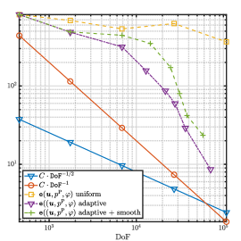
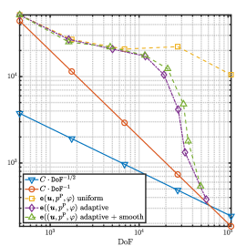
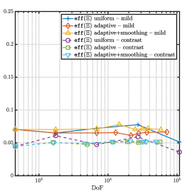
Figure 7.1. Example 2. Error decay and effectivity indexes for the convergence test on an L-shaped domain using mild and high-contrast elastic parameters with $k=1$.

7.2. Verification of a posteriori error estimates

To assess the performance of the proposed estimators, we use the L-shaped domain $\Omega=(-1,1)^{2}\setminus(0,1)^{2}$, the interface is zig-zag-shaped and going from the reentrant corner $(0,0)$ to the bottom-left corner of the domain $(-1,-1)$, and the porous domain is the one above the interface. We consider manufactured solutions with high gradients near the reentrant corner

$$\bm{u}=10^{-2}\begin{pmatrix}((x-x_{a})^{2}+(y-y_{a})^{2})^{-2/3}\\ ((x-x_{a})^{2}+(y-y_{a})^{2})^{-2/3}\end{pmatrix},\quad p^{\mathrm{P}}=((x-x_{a})^{2}+(y-y_{a})^{2})^{-2/3},$$

with $(x_{a},y_{a})=(0.01,0.01)$. We employ adaptive mesh refinement consisting in the usual steps of solving, then computing the local and global estimators, marking, refining, and smoothing. The marking of elements for refinement follows the classical Dörfler approach [21]: a given $K\in\mathcal{T}_{h}$ is marked (added to the marking set $\mathcal{M}_{h}\subset\mathcal{T}_{h}$) whenever the local error indicator $\Xi_{K}$ satisfies

$$\sum_{K\in\mathcal{M}_{h}}\Xi^{2}_{K}\geq\zeta\sum_{K\in\mathcal{T}_{h}}\Xi_{K}^{2},$$

where $\zeta$ is a user-defined bulk density parameter. All edges in the elements in $\mathcal{M}_{h}$ are marked for refinement. Additional edges are marked for the sake of closure, and an additional smoothing step (Laplacian smoothing on the refined mesh to improve the shape regularity of the new mesh) is applied before starting a new iteration of the algorithm. When computing convergence rates under adaptive mesh refinement, we use the expression

$$\texttt{r}_{(\cdot)}=-2\log(e_{(\cdot)}/\tilde{e}_{(\cdot)})[\log({\tt DoF}/\widetilde{{\tt DoF}})]^{-1}.$$

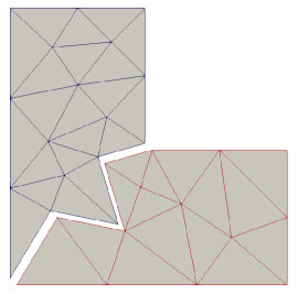
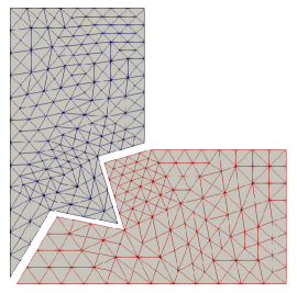
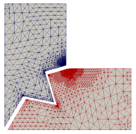
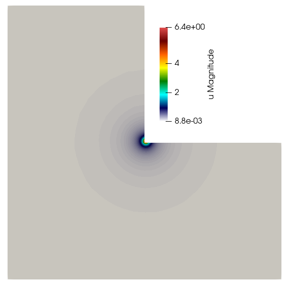
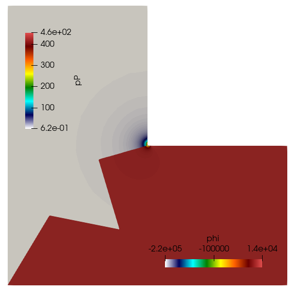
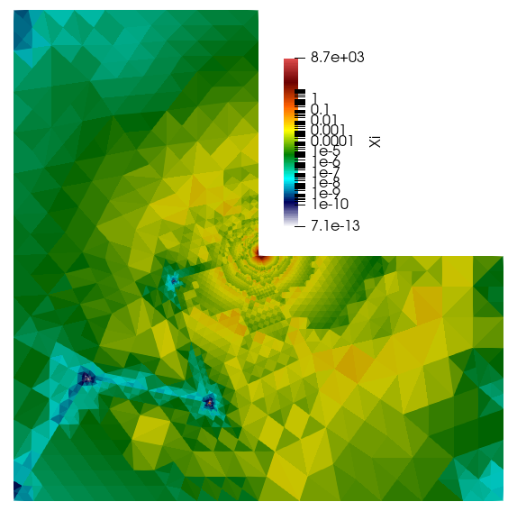
Figure 7.2. Example 2. Initial meshes for poroelastic and elastic subdomains, and meshes after 2 and 7 steps of adaptive refinement guided by $\Xi$ (top). The bottom row shows, at the finest level and for the case without mesh smoothing, the approximate global displacement, Biot fluid pressure, and the cell-wise value of the a posteriori error indicator. Here we use $k=1$.

We set the following parameter values $c_{0}=0.01$, $\alpha=0.5$, $\eta=0.01$, $\kappa=10^{-3}$ and consider two cases for the Young and Poisson moduli: first $E^{\mathrm{E}}=10$, $E^{\mathrm{P}}=100$, $\nu^{\mathrm{E}}=0.495$, $\nu^{\mathrm{P}}=0.4$, and secondly larger contrast: $E^{\mathrm{E}}=1000$, $E^{\mathrm{P}}=10$, $\nu^{\mathrm{E}}=0.499$, $\nu^{\mathrm{P}}=0.25$. Moreover, we only use the polynomial degree $k=1$, $\beta_{\bm{u}}=500$, and $\zeta=10^{-7}$. For this case we consider continuous fluid pressure approximations. The error history is presented in the left and centre panels of Figure 7.1. There we plot the error decay vs the number of degrees of freedom for the case of uniform mesh refinement, and adaptive mesh refinement with or without a smoothing step, and using the mild vs high contrast mechanical parameters. For comparison we also plot an indicative of the orders $\mathcal{O}(h)$ and $\mathcal{O}(h^{2})$ (thanks to the relation $\texttt{DoF}^{-1/d}\lesssim h\lesssim\texttt{DoF}^{-1/d}$, in 2D we take $C\,\texttt{DoF}^{-1/2}$ and $C\,\texttt{DoF}^{-1}$, respectively). We note that for high contrast parameters, the performance of the three methods is very similar. However, as the mesh is refined, for roughly the same computational cost, the two adaptive methods render a much better approximate solution. Another observation is that the effectivity indexes (plotted in the right panel) have a slightly higher oscillation than in the adaptive cases, but overall they do not show a systematic increase/decrease. We also show samples of adaptive meshes in Figure 7.2. The a posteriori error indicator correctly identifies and guides the agglomeration of elements near the zones of high gradients (the reentrant corner), plus the zones where the contrast occurs (the interface corners). The figure also portrays examples of approximate solutions together with the value of $\Xi_{K}$ locally.

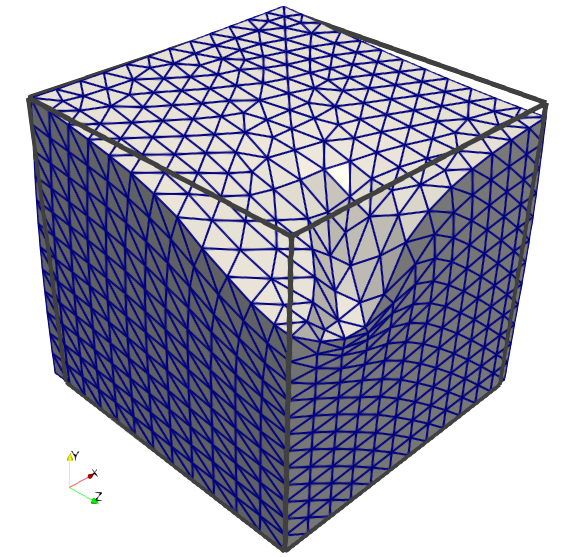
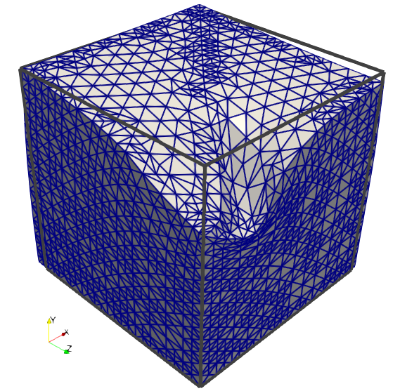
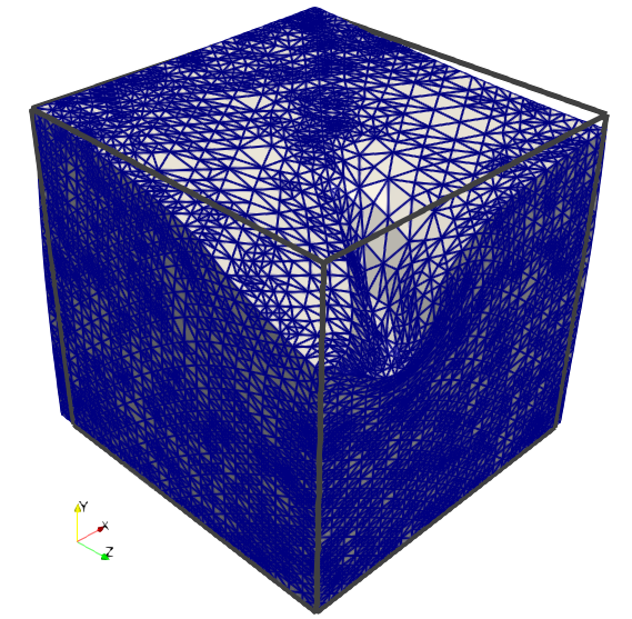
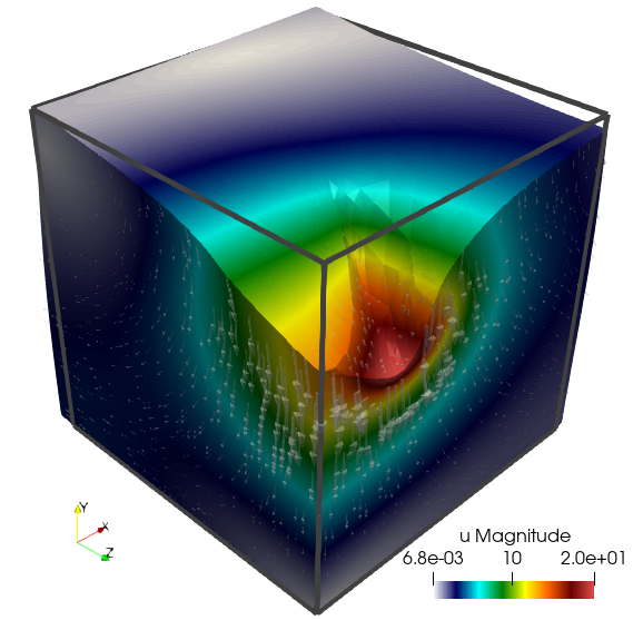
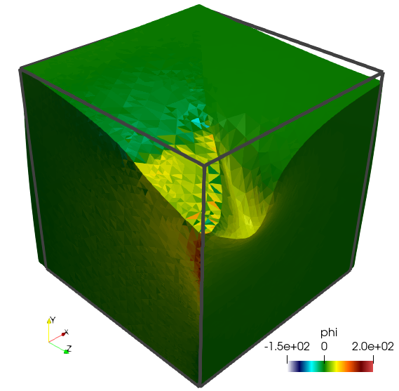
Figure 7.3. Example 3. Meshes on the deformed domain after 1, 2, and 4 steps of adaptive refinement guided by $\Xi$. The bottom row shows, at the finest level, the approximate displacement and total pressure on both subdomains, as well as the convergence of the global a posteriori error estimator.

7.3. A simple simulation of indentation in a 3D layered material

We now consider the punch problem (the drainage of a body by an induced compression loading [20, 36]). The full domain is $\Omega=(0,50)^{3}$ mm³, and it is equi-separated into elastic and poroelastic subdomains by a diagonal plane. The elastic moduli, hydromechanical coupling constants, and fluid model parameters are

$$E^{\mathrm{E}}=50\,\text{kN/mm}^{2},\quad E^{\mathrm{P}}=210\,\text{kN/mm}^{2},\quad\nu^{\mathrm{E}}=0.3,\quad\nu^{\mathrm{P}}=0.499,$$

$$\alpha=0.85,\quad c_{0}=0.1,\quad\kappa=10^{-3}\,\text{mm},\quad\eta=10^{-2}\text{kN/mm}^{2}\text{s}.$$

A normal surface load is applied on a quarter of the plane $y=50$ mm, near the corner $(0,50,50)$, where the traction has magnitude 60 N/mm². On the three planes $x=0$, $y=0$, and $z=50$ mm we prescribe zero normal displacement $\bm{u}\cdot\bm{n}=0$ together with an influx condition $\frac{\kappa}{\eta}\nabla p^{\mathrm{P}}\cdot\bm{n}=-1.7$ mm/s, and on the remainder of the boundary we set stress-free conditions for the solid phase and zero Biot pressure. Figure 7.3 shows the deformed configuration after a few steps of mesh adaptation, which clearly illustrates the jump in material properties. The meshes are more densely refined near the interface, indicating that the estimator captures correctly the error in these regions. The bottom plots suggest a difference in compliance, as observed across the interface, the deformations are more pronounced in the elastic domain. Note that the method guided by the a posteriori error estimate is particularly effective in capturing high solution gradients (of global displacement and of global total pressure). The rightmost panel of the figure also shows, in log-log scale, the decay of the global error estimator $\Xi$ vs the number of degrees of freedom, for comparison we also plot an indicative of the mesh size, for 3D, $C\,{\tt DoF}^{-\frac{1}{3}}$, which confirms that the estimator converges at least with $\mathcal{O}(h)$ to zero. Note that we are using here the lowest-order method $k=0$ with continuous fluid pressure approximation, and the mesh agglomeration parameter is chosen as $\zeta=0.02$.

7.4. A test with realistic model parameters (application to brain multiphysics)

The Biot-elasticity system described in this paper is useful in a range of applications. We show here, as an example, how it can be used to calculate the displacement in a system consisting of the wall of a penetrating vessel and the interstitium surrounding it. A proper network of vessels is shown in [28, 39], but we will do a simplified 2D illustration. Here, the vessel is T-shaped with the interstitium in a surrounding box. The boundaries are divided into Dirichlet and Neumann boundaries for both the vessel wall and the interstitium domains. The bottom boundary of the vessel wall and the top and bottom boundary of the interstitium have Dirichlet boundaries while the side boundaries for both the vessel wall and interstitium have Neumann boundaries. The mesh is shown in Figure 7.4 (top left). The displacement is driven by a pressure wave along the inside of the vessel wall, represented as a sinus wave with a period of one second and a maximum value of 1 kPa. The value is taken from [46] where the intraventricular intracranial pressure is reported to be mostly in the range 0.1-1 kPa. The vessel wall for rats are reported to be between 3.8 and 5.8 $\mu$m and the diameter of the vessels is reported to be 43 and 63 $\mu$m [11]. We choose the vessel to have a diameter of 50 $\mu$m while the vessel wall have a thickness of 5 $\mu$m in this example. The Lame parameters in the interstitium are $\mu=1$ kPa and $\lambda=1$ MPa in our example. This is in the range of $\mu=[590,2.5\cdot 10^{3}]$ Pa and $\lambda=[529,1.0\cdot 10^{11}]$ Pa given in [43]. In the vessel wall, they are chosen to be 1 MPa and 1 GPa respectively, which is similar to the reported ranges of $\mu=[3.3\cdot 10^{3},8.2\cdot 10^{5}]$ Pa and $\lambda=[3.0\cdot 10^{4},3.4\cdot 10^{12}]$ Pa given in [12, 43]. Additionally, the permeability is 100 nm² in the interstitium which within the ranges of 10 to 2490 nm² presented in [29, 43]. We use mixed boundary conditions as follows

$$[2{\mu^{\mathrm{E}}}\bm{\varepsilon}(\bm{u}^{\mathrm{E}})-\varphi^{\mathrm{E}}\mathbf{I}]\bm{n}^{\partial\Omega^{\mathrm{E}}} =0\text{ on }\Gamma^{P}_{N}$$ (7.1a)

$$\bm{u}^{\mathrm{E}} =0\text{ on }\Gamma^{P}_{D}$$ (7.1b)

$$[2{\mu^{\mathrm{P}}}\bm{\varepsilon}(\bm{u}^{\mathrm{P}})-\varphi^{\mathrm{P}}\mathbf{I}]\bm{n}^{\partial\Omega^{\mathrm{P}}} =0\text{ on }\Gamma^{P}_{N}$$ (7.1c)

$$\frac{1}{\eta}\langle\kappa\nabla p^{P}\cdot\bm{n},q^{P}\rangle_{\partial\Omega_{P}} =0\text{ on }\Gamma^{P}_{N}$$ (7.1d)

$$\bm{u}^{\mathrm{P}} =0\text{ on }\Gamma^{P}_{D},$$ (7.1e)

where $\Gamma^{E}_{N}$ and $\Gamma^{E}_{D}$ is the Neumann and Dirichlet boundaries for the vessel wall and $\Gamma^{P}_{N}$ and $\Gamma^{P}_{D}$ is the Neumann and Dirichlet boundaries for the interstitium. The previously mentioned pressure wave is described by

$$[2{\mu^{\mathrm{E}}}\bm{\varepsilon}(\bm{u}^{\mathrm{E}})-\varphi^{\mathrm{E}}\mathbf{I}]\bm{n}^{\partial\Omega^{\mathrm{E}}} =g(t)\bm{n}^{\partial\Omega^{\mathrm{E}}}\ \ \text{on}\ \Gamma_{\text{traction}},$$ (7.2)

where $\Gamma_{\text{traction}}$ is the inside of the vessel wall and $g(t)=10^{3}\cdot\sin(2\pi t)$. The simulation runs over 0.5 seconds which encompass a full expansion and contraction of the vessel wall by the pressure sine wave.

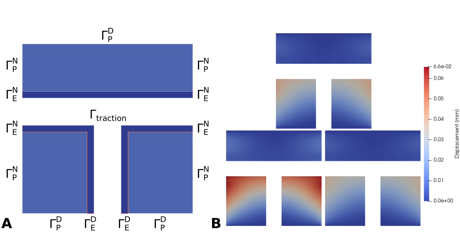
Figure 7.4. The solution of the Biot-elasticity system on a T-vessel domain. A) shows the domain with boundaries. The dark blue is the vessel wall and the lighter blue is the interstitium. The top and the bottom of the interstitium domain and the bottom of the vessel wall domain are Dirichlet boundaries, while the sides of both the interstitium and the vessel wall are Neumann boundaries. B) shows the displacement after 0.10 seconds (top), 0.25 seconds (bottom left) and 0.40 seconds (bottom right).

We time discretize the transient problem using Crank-Nicolson’s method with a constant time step $\Delta t=0.01$ seconds, and solve the problem at each step with a sparse direct solver. From the solution, Figure 7.4, we observe that the pressure wave causes the displacement to spread through the vessel wall and into the interstitium. As the pressure wave goes back to zero, the displacement in the interstitium relaxes back to zero as well. The maximum displacement is 66 $\mu$m. This displacement is quite large considering the maximum arterial wall velocity is 18-25 $\mu$m/s in mice, as reported in [40].

7.5. Evaluation of preconditioning robustness

We thoroughly evaluated the robustness of $\mathcal{P}_{h}$ in (6.4) for a wide span of physical parameter-value ranges of interest, different mesh resolutions, H(div)-conforming approximations for the displacements (in particular, BDM and Raviart–Thomas), different rectangular domain shapes, and elastic and poroelastic rectangular subdomain shapes. Overall, our results confirm an asymptotically constant number of MINRES iterations with mesh resolution even with material parameters that exhibit very large jumps accross the interface (e.g., we tested up to 3 orders of magnitude jumps in $\mu$ and $\lambda$), and/or very small or very large values (e.g., $\kappa\in[10^{-3},10^{-5},10^{-7}]\text{ m}^{2}$; $\lambda,\mu\in[1,10^{3},10^{6},10^{9}]$ Pa), including the extreme cases of near incompressibility, near impermeability, and near zero storativity. We note, however, that the value of the penalty parameter $\beta_{\bm{u}}$ has to be chosen carefully (typically via numerical experimentation), as it can have a significant impact on preconditioner efficiency.

For conciseness, in this section, we only show results for the particularly challenging (and realistic) combination of physical parameter values corresponding to the problem in Section 7.4. We use the upper part of the domain in this problem, namely the rectangular domain $\Omega=[0,0.25]\times[0.17,0.25]$, with elastic subdomain spanning the thin stripe $[0,0.25]\times[0.17,0.1705]$. As usual, the poroelastic domain is defined as the complement of the elastic domain. We used a triangular uniform mesh generator parametrizable by the number of layers of triangles in the thinner dimension of the elastic domain, which we refer to as $\ell$. Note that $h=0.05/\ell$. We tested in particular with three mesh resolutions corresponding to $\ell=2,4,8$. We solve problem (3.5) with the known manufactured solution described in Section 7.1. We report results only for BDM with $k=0$, although we stress that the number of iterations obtained for Raviart-Thomas with $k=1$ were very similar to those reported herein. The preconditioned MINRES solver is used in conjunction with $\mathcal{P}_{h}$ in (6.4), and convergence is claimed whenever the Euclidean norm of the (unpreconditioned) residual of the whole system is reduced by a factor of $10^{6}$. The action of the preconditioner was computed by LU decomposition in all cases. As an illustration of the challenge at hand, for $\ell=2$, $\beta_{\bm{u}}=20$, the condition number of the unpreconditioned system (3.5) is approximately as large as $1.25\times 10^{26}$ (as computed by the cond Julia function). By a suitable scaling of the system, this large number could be reduced to $1.25\times 10^{14}$ (i.e., by 12 orders of magnitude). In particular, we scale (2.1a) and (2.1d) with $1/\max(\mu^{\mathrm{P}},\mu^{\mathrm{E}})$ and solve for the scaled pressures $\varphi^{\mathrm{P,E}}\leftarrow\varphi^{\mathrm{P,E}}/\max(\mu^{\mathrm{P}},\mu^{\mathrm{E}})$ and $p^{\mathrm{P}}\leftarrow p^{\mathrm{P}}/\max(\mu^{\mathrm{P}},\mu^{\mathrm{E}})$; see also scale_parameters function in [7] for full details. We stress that, while the number of preconditioned MINRES iterations to solve the original and scaled systems was almost equivalent in all cases tested, we observed a much more reliable behaviour of the error curves for the scaled equations, in particular, under the assumption of a relatively coarse fixed residual tolerance. Thus, in the sequel, we report the errors we obtained in the presence of such an scaling. Finally, in order to study the dependence of the number of iterations and error on the penalisation parameter $\beta_{\bm{u}}$, we tested with different values of $\beta_{\bm{u}}\in[10,5000]$.

In Figure 7.5 (left), we report the number of preconditioned MINRES iterations versus number of degrees of freedom. While the value chosen for $\beta_{\bm{u}}$ has an impact on the number of iterations for fixed mesh resolution, we can observe nevertheless an asymptotically constant number of iterations with mesh resolution for most of the values of $\beta_{\bm{u}}$ tested. This can be better observed in Figure 7.5 (right), where we report the number of iterations versus $\beta_{\bm{u}}$ for different values of mesh resolution $\ell$; the number of iterations to achieve convergence is approximately constant with mesh resolution except for values of $\beta_{\bm{u}}$ within $[50,200]$. In order to have a more complete picture, in the curves labeled as “solver=pminres” in Figure 7.6, we report the errors in the displacements (left), fluid pressure (center), and global pressure (right) versus $\beta_{\bm{u}}$, obtained with the preconditioned MINRES solver. As a reference, in the curves labeled as “solver=lu” in Figure 7.6, we report the corresponding errors obtained with a robust sparse direct solver (UMFPACK). We can observe that the value of $\beta_{\bm{u}}$ has an impact on the error obtained, particularly noticeable in the case of the preconditioned MINRES solver; only for the smallest value of $\beta_{\bm{u}}=10$, the accuracy of the sparse direct solver can be matched for all unknowns. We have checked that, as expected, as we use finer residual tolerances, the error curves for the MINRES solver become closer to those obtained with the sparse direct solver (at the price of some more iterations).

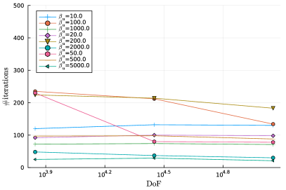
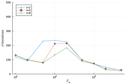
Figure 7.5. Number of preconditioned MINRES iterations versus number of degrees of freedom for different values of $\beta_{\bm{u}}$ (left) and versus $\beta_{\bm{u}}$ for different values of mesh resolution $\ell$ (right).

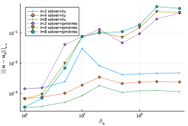
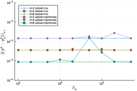
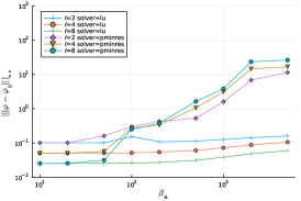
Figure 7.6. Error in the displacements (left), fluid pressure (center), and global pressure (right) versus $\beta_{\bm{u}}$ for different values of mesh resolution $\ell$.

References

- [1] Elyes Ahmed, Florin Adrian Radu and Jan Martin Nordbotten “Adaptive poromechanics computations based on a posteriori error estimates for fully mixed formulations of Biot’s consolidation model” In Computer Methods in Applied Mechanics and Engineering 347, 2019, pp. 264–294
- [2] M.. Alnæs et al. “The FEniCS Project Version 1.5” In Archive of Numerical Software 3.100, 2015, pp. 9–23
- [3] P.. Amestoy, I.. Duff, J. Koster and J.-Y. L’Excellent “A Fully Asynchronous Multifrontal Solver Using Distributed Dynamic Scheduling” In SIAM Journal on Matrix Analysis and Applications 23.1, 2001, pp. 15–41
- [4] Veronica Anaya, Arbaz Khan, David Mora and Ricardo Ruiz-Baier “Robust a posteriori error analysis for rotation-based formulations of the elasticity/poroelasticity coupling” In SIAM Journal on Scientific Computing 44.4, 2022, pp. B964–B995
- [5] Verónica Anaya, Zoa De Wijn, Bryan Gómez-Vargas, David Mora and Ricardo Ruiz-Baier “Rotation-based mixed formulations for an elasticity-poroelasticity interface problem” In SIAM Journal on Scientific Computing 42.1, 2020, pp. B225–B249
- [6] Douglas N Arnold “An interior penalty finite element method with discontinuous elements” In SIAM Journal on Numerical Analysis 19.4 SIAM, 1982, pp. 742–760
- [7] S. Badia et al. “Software used in “Efficient and reliable divergence-conforming methods for an elasticity-poroelasticity interface problem””, https://doi.org/10.5281/zenodo.8017784 URL: https://doi.org/10.5281/zenodo.8017784
- [8] Santiago Badia, Alberto F. Martín and Francesc Verdugo “GridapDistributed: a massively parallel finite element toolbox in Julia” In Journal of Open Source Software 7.74 The Open Journal, 2022, pp. 4157 URL: https://doi.org/10.21105/joss.04157
- [9] Santiago Badia and Francesc Verdugo “Gridap: An extensible Finite Element toolbox in Julia” In Journal of Open Source Software 5.52 The Open Journal, 2020, pp. e2520 URL: https://doi.org/10.21105/joss.02520
- [10] Francesco Ballarin “multiphenics – easy prototyping of multiphysics problems in FEniCS” Accessed: 2022-03-10, https://mathlab.sissa.it/multiphenics
- [11] Gary L Baumbach, Philip B Dobrin, Michael N Hart and Donald D Heistad “Mechanics of cerebral arterioles in hypertensive rats.” In Circulation research 62.1 Am Heart Assoc, 1988, pp. 56–64
- [12] DH Bergel “The static elastic properties of the arterial wall” In The Journal of physiology 156.3 Wiley-Blackwell, 1961, pp. 445
- [13] Daniele Boffi, Franco Brezzi and Michel Fortin “Mixed Finite Element Methods and Applications” Berlin: Springer-Verlag, 2013
- [14] Susanne C Brenner “Korn’s inequalities for piecewise H1 vector fields” In Mathematics of Computation JSTOR, 2004, pp. 1067–1087
- [15] Franco Brezzi, Jim Douglas and L Donatella Marini “Two families of mixed finite elements for second order elliptic problems” In Numerische Mathematik 47.2 Springer, 1985, pp. 217–235
- [16] Raimund Bürger, Arbaz Khan, Paul E. Méndez and Ricardo Ruiz-Baier “Divergence-conforming methods for transient doubly-diffusive flows: A priori and a posteriori error analysis” In Arxiv Preprint arXiv:2102.05819, 2021
- [17] Raimund Bürger, Paul E. Méndez and Ricardo Ruiz-Baier “On H(div)-conforming methods for double-diffusion equations in porous media” In SIAM Journal on Numerical Analysis 57.3, 2019, pp. 1318–1343
- [18] Pablo GS Carvalho, Philippe RB Devloo and Sônia M Gomes “On the use of divergence balanced H(div)-L2 pair of approximation spaces for divergence-free and robust simulations of Stokes, coupled Stokes–Darcy and Brinkman problems” In Mathematics and Computers in Simulation 170 Elsevier, 2020, pp. 51–78
- [19] Yumei Chen, Feiteng Huang and Xiaoping Xie “H(div) conforming finite element methods for the coupled Stokes and Darcy problem” In Journal of Computational and Applied Mathematics 235.15 Elsevier, 2011, pp. 4337–4349
- [20] Mertcan Cihan, Blaž Hudobivnik, Fadi Aldakheel and Peter Wriggers “3D mixed virtual element formulation for dynamic elasto-plastic analysis” In Computational Mechanics 68.3 Springer, 2021, pp. 1–18
- [21] Willy Dörfler “A Convergent Adaptive Algorithm for Poisson’s Equation” In SIAM Journal on Numerical Analysis 33.3, 1996, pp. 1106–1124
- [22] Emilie Eliseussen, Marie E. Rognes and Travis B. Thompson “A-posteriori error estimation and adaptivity for multiple-network poroelasticity” In Arxiv Preprint arXiv:2111.13456, 2021
- [23] A Ern and J.-L. Guermond “Theory and Practice of Finite Elements” Appl. Math. Sci. 159, Springer-Verlag, New York, 2004
- [24] Guosheng Fu and Christoph Lehrenfeld “A strongly conservative hybrid DG/mixed FEM for the coupling of Stokes and Darcy flow” In Journal of Scientific Computing 77.3 Springer, 2018, pp. 1605–1620
- [25] V. Girault, G. Pencheva, M.. Wheeler and T. Wildey “Domain decomposition for poroelasticity and elasticity with DG jumps and mortars” In Mathematical Models and Methods in Applied Sciences 21.01, 2011, pp. 169–213
- [26] Vivette Girault, Xueying Lu and Mary F. Wheeler “A posteriori error estimates for Biot system using Enriched Galerkin for flow” In Computer Methods in Applied Mechanics and Engineering 369, 2020, pp. e113185
- [27] Vivette Girault, Mary F Wheeler, Benjamin Ganis and Mark E Mear “A lubrication fracture model in a poro-elastic medium” In Mathematical Models and Methods in Applied Sciences 25.04 World Scientific, 2015, pp. 587–645
- [28] Florian Goirand, Tanguy Le Borgne and Sylvie Lorthois “Network-driven anomalous transport is a fundamental component of brain microvascular dysfunction” In Nature communications 12.1 Nature Publishing Group, 2021, pp. 1–11
- [29] Karl Erik Holter et al. “Interstitial solute transport in 3D reconstructed neuropil occurs by diffusion rather than bulk flow” In Proceedings of the National Academy of Sciences 114.37 National Acad Sciences, 2017, pp. 9894–9899
- [30] Qingguo Hong and Johannes Kraus “Uniformly stable discontinuous Galerkin discretization and robust iterative solution methods for the Brinkman problem” In SIAM Journal on Numerical Analysis 54.5 SIAM, 2016, pp. 2750–2774
- [31] Qingguo Hong, Johannes Kraus, Maria Lymbery and Fadi Philo “Conservative discretizations and parameter-robust preconditioners for Biot and multiple-network flux-based poroelasticity models” In Numerical Linear Algebra with Applications 26.4 Wiley Online Library, 2019, pp. e2242
- [32] Qingguo Hong, Johannes Kraus, Jinchao Xu and Ludmil Zikatanov “A robust multigrid method for discontinuous Galerkin discretizations of Stokes and linear elasticity equations” In Numerische Mathematik 132.1 Springer, 2016, pp. 23–49
- [33] Guido Kanschat and Béatrice Riviere “A strongly conservative finite element method for the coupling of Stokes and Darcy flow” In Journal of Computational Physics 229.17 Elsevier, 2010, pp. 5933–5943
- [34] Guido Kanschat and Beatrice Riviere “A finite element method with strong mass conservation for Biot’s linear consolidation model” In Journal of Scientific Computing 77.3 Springer, 2018, pp. 1762–1779
- [35] Juho Könnö and Rolf Stenberg “H(div)-conforming finite elements for the Brinkman problem” In Mathematical Models and Methods in Applied Sciences 21.11 World Scientific, 2011, pp. 2227–2248
- [36] Sarvesh Kumar, Ricardo Oyarzúa, Ricardo Ruiz-Baier and Ruchi Sandilya “Conservative discontinuous finite volume and mixed schemes for a new four-field formulation in poroelasticity” In ESAIM: Mathematical Modelling and Numerical Analysis 54.1, 2020, pp. 273–299
- [37] J. Lee, Kent-Andre Mardal and R. Winther “Parameter-Robust Discretization and Preconditioning of Biot’s Consolidation Model” In SIAM Journal on Scientific Computing 39.1, 2017, pp. A1–A24
- [38] Yuwen Li and Ludmil T Zikatanov “Residual-based a posteriori error estimates of mixed methods for a three-field Biot’s consolidation model” In IMA Journal of Numerical Analysis 42.1 Oxford University Press, 2022, pp. 620–648
- [39] Sylvie Lorthois, Florian Goirand and Tanguy Le Borgne “Raw data for “Network-driven anomalous transport is a fundamental component of brain microvascular dysfunction”, Nature Communications, 12, 7295 (2021)” Harvard Dataverse, 2021 URL: https://doi.org/10.7910/DVN/QJDUUA
- [40] Humberto Mestre et al. “Flow of cerebrospinal fluid is driven by arterial pulsations and is reduced in hypertension” In Nature communications 9.1 Nature Publishing Group UK London, 2018, pp. 4878
- [41] Andro Mikelić and Mary F. Wheeler “On the interface law between a deformable porous medium containing a viscous fluid and an elastic body” In Mathematical Models and Methods in Applied Sciences 22.11, 2012, pp. 1250031
- [42] Maxim A Olshanskii, Jörg Peters and Arnold Reusken “Uniform preconditioners for a parameter dependent saddle point problem with application to generalized Stokes interface equations” In Numerische Mathematik 105 Springer-Verlag, 2006, pp. 159–191
- [43] Joshua H Smith and Joseph AC Humphrey “Interstitial transport and transvascular fluid exchange during infusion into brain and tumor tissue” In Microvascular research 73.1 Elsevier, 2007, pp. 58–73
- [44] Francesc Verdugo and Santiago Badia “The software design of Gridap: A Finite Element package based on the Julia JIT compiler” In Computer Physics Communications 276 Elsevier BV, 2022, pp. 108341 URL: https://doi.org/10.1016/j.cpc.2022.108341
- [45] Rüdiger Verfürth “A Posteriori Error Estimation Techniques for Finite Element Methods” In A Posteriori Error Estim. Tech. Finite Elem. Methods Oxford: Oxford University Press, 2013
- [46] Vegard Vinje et al. “Respiratory influence on cerebrospinal fluid flow–a computational study based on long-term intracranial pressure measurements” In Scientific reports 9.1 Nature Publishing Group UK London, 2019, pp. 9732
- [47] Yuping Zeng, Mingchao Cai and Feng Wang “An H(div)-conforming Finite Element Method for Biot’s Consolidation Model” In East Asian Journal on Applied Mathematics 9.3 NIH Public Access, 2019, pp. 558
- [48] Yuping Zeng, Zhifeng Weng and Fen Liang “Convergence Analysis of H(div)-Conforming Finite Element Methods for a Nonlinear Poroelasticity Problem” In Discrete Dynamics in Nature and Society 2020 Hindawi, 2020, pp. 9494389