Deep Learning-based Auto-encoder for Time-offset Faster-than-Nyquist Downlink NOMA with Timing Errors and Imperfect CSI

Abstract

In this paper, we examine the encoding and decoding of transmitted sequences for downlink time-offset with faster than Nyquist signaling NOMA (T-NOMA). As a baseline, we use the singular value decomposition (SVD)-based scheme proposed in previous studies for encoding and decoding. Even though this SVD-based scheme provides reliable communication, its time complexity increases quadratically with the sequence length. We propose a convolutional neural network (CNN) auto-encoder (AE) for encoding and decoding with linear time complexity. We explain the design of the encoder and decoder architectures and the training criteria. By examining several variants of the CNN AE, we show that it can achieve an excellent trade-off between performance and complexity. A proposed CNN AE outperforms the SVD method using a lower implementation complexity by approximately 2 dB in a T-NOMA system with two users assuming no timing offset errors or channel state information estimation errors. In the presence of channel state information (CSI) error variance of 1$\%$ and uniform timing error at $\pm$4% of the symbol interval, the proposed CNN AE provides up to 10 dB SNR gain over the SVD method. We also propose a novel modified training objective function consisting of a linear combination of the traditionally used cross-entropy (CE) loss function and a closed-form expression for the bit error rate (BER) called the Q-loss function. Simulations show that the modified loss function achieves SNR gains of up to 1 dB over the CE loss function alone. Finally, we investigate several novel CNN architectures for both the encoder and decoder components of the AE that employ additional linear feed-forward connections between the CNN stages; experiments show that these architectural innovations achieve additional SNR gains of up to 2.2 dB over the standard serial CNN AE architecture.

I Introduction

Next-generation wireless standards will support more users, reduce latencies, facilitate high data rates, and improve reliability [1]. Current wireless standards employ orthogonal multiple access (OMA) techniques, where distinct users can only communicate over orthogonal resources. An example is orthogonal frequency-division multiple access (OFDMA), which assigns orthogonal sub-carriers to different users to limit inter-user interference (IUI) [2]. However, OMA techniques are sub-optimal in terms of achieving the channel capacity [3]. With non-orthogonal multiple access (NOMA), multiple users can communicate over the same resource element (frequency sub-carriers, time slots, or spreading codes) [1, 4].

I-A Downlink Power-domain NOMA (P-NOMA)

Power-domain NOMA (P-NOMA) assigns different signal powers to different users [5, 1, 6]. Consider a downlink channel where a base station communicates to two users over the same channel. In P-NOMA, the base station transmits the superposition of two non-orthogonal signal components. Each component is intended for a particular recipient. Assume that User 1 has better channel conditions than User 2. To recover their own message, User 1 decodes the message of User 2 first. Ideally, at User 1, User 2’s message can be decoded correctly and removed from the superposition due to User 1’ better channel conditions. Then, User 1 can decode their respective message without interference. User 2 decodes their own message with interference from User 1’s message, which cannot be canceled due to User 2’ worse channel conditions. P-NOMA enables multiple users to communicate over orthogonal resources via superposition encoding and successive interference cancellation. For the two-user Gaussian broadcast channel, the described P-NOMA scheme can achieve the channel capacity [7, pp. 509–595].

I-B Faster than Nyquist Signaling

Typically, the transmission pulse satisfies the Nyquist intersymbol interference (ISI) criterion. The time-domain Nyquist criterion for a pulse $h(t)$ is that $h(0)=1$ and $h(nT)=0$, where $T$ is the symbol interval and $n$ is an integer[8]. If the noise-free pulse shape after matched filtering satisfies the Nyquist-pulse criterion, then by sampling the matched filter output at the Nyquist data transmission rate, the received signal does not experience inter-symbol interference (ISI). Hence, maximum likelihood symbol detection can be achieved using symbol-by-symbol processing without considering channel memory, resulting in simpler implementations. Suppose data is transmitted at a rate faster than the Nyquist transmission rate. In that case, the received signal experiences ISI, and symbol-by-symbol processing no longer provides maximum likelihood detection performance. However, with appropriate data processing to account for this ISI, faster than Nyquist signaling enables higher Shannon capacities, improved bandwidth efficiencies, and multiple user broadcasting [8, 9]. This paper considers encoding and decoding schemes for FTN broadcast signaling in downlink NOMA.

I-C Time-offset with faster than Nyquist Signaling NOMA (T-NOMA)

Time-offset with faster than Nyquist signaling NOMA (T-NOMA) introduces timing offsets between the continuous-time signals intended for different users and transmits the superposition of such signals [9, 5, 10]. For decoding in T-NOMA, the received time-domain signal is sampled at a faster rate than the Nyquist transmission rate. T-NOMA leverages faster than Nyquist (FTN) signaling for the broadcast channel, as proposed by Kim and Bajcsy in [9]. FTN broadcasting achieves the channel capacity of the broadcast channel. Furthermore, maximizing the sum rate in T-NOMA facilitates fairness among users, contrary to P-NOMA [5].

I-D Auto-encoder

The auto-encoder (AE) was first proposed in [11] as a non-linear generalization of principal component analysis. The AE consists of a neural network-based encoder and decoder that are trained jointly to minimize an objective function. For example, in image reconstruction, the encoder learns efficient representations of the input images and the decoder learns to recover the images from such representations. The mean squared error (MSE) loss function is commonly used for training the AE. The work in [12] by O’Shea and Hoydis is among the first to illustrate the application of AEs to wireless channels, including a two-user interference channel and a single user fading channel. The AE described in [12] accepts the messages from distinct users for transmission. The encoder encodes the messages such that the decoder can reliably decode the transmitted messages.

I-E Relevant Studies on Using an Auto-encoder for NOMA

In T-NOMA, one of the major challenges is the design of efficient encoding and decoding schemes for data recovery. A linear singular value decomposition (SVD) based encoding and decoding scheme is proposed in [5, 13, 14] for T-NOMA. In, [5, 13], the authors consider achievable rates for P-NOMA and the SVD scheme in T-NOMA. This scheme enables the receiver to decouple the superposition signal sequence into independent channels with minimal interference assuming accurate knowledge of the timing offset at the transceivers. However, the SVD’s encoding and decoding complexities are quadratic in the length of the transmitted sequence. In [14], Chaki and Sugiura propose a linear encoding and decoding scheme for T-NOMA based on the SVD. Their results show that the proposed scheme achieves competitive BERs and spectral efficiencies using the raised cosine filter compared with the rectangular filter. In this paper, we propose a convolutional neural network (CNN) auto-encoder (AE) for T-NOMA whose complexity is linear in the length of the transmitted sequence and is more resilient to errors in the timing offset.

In [15], Gui et al. propose an AE consisting of fully connected and long short-term memory (LSTM) layers for P-NOMA. To address imperfect interference cancellation, Kang et al. in [16] propose an AE for encoding and decoding in P-NOMA using fully-connected neural networks (FNNs). In [17], Sun et al. propose using a FNN for detection and message passing with another FNN decoder in P-NOMA. In [18], Ye et al. propose using a deep neural network (DNN) AE consisting of FNNs for P-NOMA. The encoder encodes the messages over the available orthogonal resource elements, and the decoder recovers the transmitted messages. In [19], Luo et al. propose an AE to learn a sparse code multiple access for downlink NOMA. Their results indicate that the AE outperforms previously proposed sparse codes in terms of the average bit error rate (BER) and complexity. In [20], Miuccio et al. propose integrating a generative adversarial network (GAN) with an auto-encoder for sparse code multiple access code design for NOMA. Their results show improved BER performance, especially at low SNRs. In [21], Han et al. propose a deep AE for sparse code multiple access where both the resource allocation and bit-to-symbol mapping are jointly optimized. The authors show ttheir proposed approach achieves improvements in BER performance that are competitive with a baseline one-user channel.

I-F Summary of Proposed Methods

Despite the recent progress in deep learning systems for NOMA, the proposed approaches assume NOMA with Nyquist rate transmission. When considering T-NOMA, the AE must consider the full length of the transmitted sequence for encoding and decoding. Hence, the AE must be designed such that long sequences are processed efficiently.

The novel contributions of this paper are summarized as follows.

1. We propose novel CNN AE architectures for the T-NOMA downlink channel with linear complexity in the length of the transmitted sequence. To the best of the authors’ knowledge, no previous studies have examined the design of AEs for T-NOMA. We show that the proposed AE design outperforms the SVD-based scheme in terms of detection accuracy, robustness, and efficiency.

2. We propose a novel objective loss function that combines conventional cross-entropy loss with a Q-function-based term that estimates the error probability using the mean and variance of empirical log-likelihood ratios (LLRs). We show that this modification of the loss function can result in better BERs given the same neural network architecture.

3. We derive the ergodic achievable rates for P-NOMA. We compare the achievable rates for P-NOMA with those for the SVD scheme in T-NOMA. Further, we provide analytical expressions for the BER of P-NOMA. We provide a BER comparison between P-NOMA, the SVD scheme in T-NOMA, and CNN AE architectures for T-NOMA.

4. We evaluate the impact of timing error and imperfect channel state information (CSI) on the performance of the proposed and baseline systems. We show that such impairments result in data-dependent noise seen at the receiver. To improve the robustness of the CNN AE to this data-dependent noise, we propose a multilayer perceptron (MLP) power allocator (MLP-PA) at the transmitter and an MLP CSI transformer (MLP-T) at the receiver. We show that the MLP components improve the performance of the CNN AE. When BPSK modulation is used in a two-user T-NOMA system, we demonstrate twice the throughput of a single user system given the same average power per user.

II System Model

II-A Downlink Channel Model for T-NOMA

Let $x_{k}[n]$ denote the modulation symbol intended for user $k$ at time $n$, $T$ be the symbol interval, $p(t)$ be the truncated pulse shape spanning $N_{p}$ symbols for the duration $T_{p}=N_{p}T$, $N$ be the block length, and $P_{k,n}$ be the transmit power allocated for $n$th symbol intended for the $k$th user. Then, the complex baseband component of the transmitted signal intended for user $k$ is given by [5]:

$$x_{k}(t)=\sum_{n=1}^{N}\sqrt{P_{k,n}}x_{k}[n]p(t-(n-1)T).$$ (1)

Let $K$ denote the number of users, and $\tau_{k}$ denote the time offset introduced in the signal intended for user $k$. The base station transmits the superposition signal $x_{\text{transmit}}=\sum_{k=1}^{K}x_{k}(t-\tau_{k}).$ If $h_{r}$ is the flat fading channel complex coefficient for the $N$ symbols when communicating to user $r$, then user $r$’s received signal is given by:

$$y^{r}(t)=h_{r}\sum_{k=1}^{K}x_{k}(t-\tau_{k})+n^{r}(t),$$ (2)

where $n^{r}(t)$ is complex additive white Gaussian noise (CAWGN) representing the electronics noise at the user equipment with power spectral density $N_{0}$.

As shown in [9, 5], the sufficient statistics at the receiver for user $r$ for estimating $x_{k}[n]$ are given by:

$$y_{l}^{r}[m] =\int_{-\infty}^{\infty}y^{r}(u)p(u-(m-1)T-\tau_{l})du=(y^{r}(t)*p(-t))|_{t=(m-1)T+\tau_{l}},$$ (3)

$$\quad r=1,\ldots,K,\leavevmode\nobreak\ l=1,\ldots,K,\leavevmode\nobreak\ m=1,\ldots,N.$$

By defining $g(t)\triangleq p(t)*p(-t)$ and $g_{l,k}[m-n]\triangleq g((m-n)T+(\tau_{l}-\tau_{k}))$, we can write the discrete-time sufficient statistics as:

$$y_{l}^{r}[m]=h_{r}\sum_{k=1}^{K}\sum_{n=1}^{N}\sqrt{P_{k,n}}g_{l,k}[m-n]x_{k}[n]+n_{l}^{r}[m].$$ (4)

Appendix A illustrates the correlator receivers for obtaining the sufficient statistics with two users and an offset of $T/2$.

Without loss of generality, we assume $\mathbf{E}\{|x_{k}[m]|^{2}\}=1$, $\mathbf{E}\{|h_{r}|^{2}\}=1$, and $\sum_{m}{g}_{l,k}^{2}[m]=1$. Let $P_{k}$ denote the average power allocated to user $k$. Then, $P_{k}=(1/N)\sum_{n}P_{k,n}$, and the average total power budget is $P=\sum_{k}P_{k}$. The correlated noise $n_{l}^{r}[m]=n(t)*p(t)|_{t=(m-1)T+\tau_{l}}$ has the auto-correlation given by:

$$R_{l}^{r}[m]=\mathbf{E}[n_{l}^{r}[n+m]n_{l}^{r*}[n]]=\begin{cases}N_{0}g_{l,r}[m],&\text{if $m\leq N_{p}$},\\ 0,&\text{otherwise.}\end{cases}$$ (5)

II-B SVD-based Baseline

The received signal in (4) can be written in matrix form as follows. Let $\mathbf{y}^{r}_{l}=[y_{l}^{r}[1],\ldots,y_{l}^{r}[N]]^{T}$, $\mathbf{y}^{r}=[\mathbf{y}^{rT}_{1},\ldots,\mathbf{y}^{rT}_{K}]^{T}$, and $\mathbf{n}^{r}$ be similarly defined. The transmitted symbols are interleaved such that $\mathbf{x}=[\mathbf{x}[1],\ldots,\mathbf{x}[N]]^{T}$, where $\mathbf{x}[n]=[x_{1}[n],\ldots,x_{K}[n]]$ [9]. When computing the convolution between $\mathbf{x}$ and $\mathbf{g}_{l,k}$, only the $N_{v}=N-N_{p}+1$ valid outputs that do not require zero padding are considered. Then, $\mathbf{y}^{r}$ is given by:

$$\mathbf{y}^{r}=h_{r}\mathbf{G}\mathbf{P}\mathbf{x}+\mathbf{n}^{r},$$ (6)

where $\mathbf{G}$ is a $KN_{v}\times KN$ doubly-block Toeplitz matrix representing the superposition and convolutions using $\mathbf{g}_{l,k}$s, and $\mathbf{P}=\text{diag}([P_{k,n}])$.

The transmitter can encode the transmitted symbols by premultiplying $\mathbf{Px}$ by a unitary matrix $\mathbf{U}_{\text{transmit}}$. Then, the receiver premultiplies the received signal sequence by the unitary matrix $\mathbf{U}_{\text{receive}}$. Using the appropriate choice of the encoding and post-processing matrices, the superposition channel can be decoupled into separate channels. Assuming $\mathbf{G}$ has rank $r_{\mathbf{G}}$, an SVD of $\mathbf{G}$ is given by $\mathbf{G}=\mathbf{U}\mathbf{\Lambda}\mathbf{V}^{H}$, where $\mathbf{U}$ and $\mathbf{V}$ are unitary matrices such that $\mathbf{U}^{H}\mathbf{U}=\mathbf{V}^{H}\mathbf{V}=\mathbf{I}_{r_{\mathbf{G}}\times r_{\mathbf{G}}}$, and $\mathbf{\Lambda}$ is a rectangular diagonal matrix with $r_{\mathbf{G}}$ non-zero singular values. If $\mathbf{U}_{\text{transmit}}=\mathbf{V}$ and $\mathbf{U}_{\text{receive}}=\mathbf{U}^{H}$, then, ideally, the received signal can be decoupled into $r_{\mathbf{G}}$ channels without IUI as follows:

$$\mathbf{U}^{H}\mathbf{y}^{r}=h_{r}\mathbf{\Lambda}\mathbf{P}\mathbf{x}+\mathbf{U}^{H}\mathbf{n}^{r}.$$ (7)

From (7), the diagonal matrix $\mathbf{\Lambda}$ premultiplies $\mathbf{P}\mathbf{x}$, resulting in $r_{\mathbf{G}}\leq KN_{v}$ decoupled sub-channels seen by the receiver. Ideally, the $r_{\mathbf{G}}$ sub-channels do not contain ISI or IUI. Thus, the detection does not use SIC, which can be difficult to realize in practice. The SVD encoding and decoding applies linear operations on the discrete transmitted and received samples, respectively. The encoding and decoding complexity of the SVD is $O(KN_{v})$ as discussed in Subsection IV-C.

II-C Sources of Data-dependent Noise

We illustrate that errors in the timing offsets cause data-dependent noise. Consider the two-user downlink channel where the intended difference between the timing offsets is $\tau_{\text{design}}=\tau_{1,\text{design}}-\tau_{2,\text{design}}$. Without loss of generality, we assume that $\tau_{2,\text{design}}=0$. Due to propagation delays, mobility of users, and sample time errors, the actual time offset is $\tau=\tau_{\text{design}}+\epsilon$, where $\epsilon$ is the timing error. We assume that $\epsilon$ is zero-mean and uniformly distributed over a width $w>0$, i.e., $\epsilon\sim U(-w/2,w/2)$. Because of the timing error, the transmitted symbols undergo the matrix transformation $\mathbf{G}_{\epsilon}$ instead of $\mathbf{G}$. Let $\mathbf{G}_{\epsilon}=\mathbf{U}_{\epsilon}\mathbf{\Lambda}_{\epsilon}\mathbf{V}_{\epsilon}^{H}$ be an SVD of $\mathbf{G}_{\epsilon}$. Let $\mathbf{U}^{H}\mathbf{U}_{\epsilon}=\mathbf{I}+\mathbf{E}_{u}$ and $\mathbf{V}^{H}_{\epsilon}\mathbf{V}=\mathbf{I}+\mathbf{E}_{v}$. Then, the encoding and decoding by the SVD gives:

$$\mathbf{U}^{H}\mathbf{y}^{r} =h_{r}\mathbf{U}^{H}\mathbf{G}_{\epsilon}\mathbf{V}\mathbf{Px}+\mathbf{U}^{H}\mathbf{n}^{r}=h_{r}(\mathbf{I}+\mathbf{E}_{u})\mathbf{\Lambda}_{\epsilon}(\mathbf{I}+\mathbf{E}_{v})\mathbf{Px}+\mathbf{U}^{H}\mathbf{n}^{r}$$ (8)

$$=h_{r}\mathbf{\Lambda}_{\epsilon}\mathbf{Px}+h_{r}\mathbf{n}_{\epsilon}(\mathbf{x})+\mathbf{U}^{H}\mathbf{n}^{r},$$ (9)

where $\mathbf{n}_{\epsilon}(\mathbf{x})\triangleq(\mathbf{\Lambda_{\epsilon}}\mathbf{E}_{v}+\mathbf{E}_{u}\mathbf{\Lambda}_{\epsilon}+\mathbf{E}_{u}\mathbf{\Lambda}_{\epsilon}\mathbf{E}_{v})\mathbf{Px}$ is the data-dependent noise term due to the error $\epsilon$ on the timing offset.

Another source of data-dependent noise is the estimation error of $h_{r}$. To correctly detect the transmitted symbols, $h_{r}$ is usually estimated by the receiver. To enable estimating $h_{r}$ at the receiver, a pilot symbol is transmitted by the base station to the user. This pilot symbol is known at the receiver by design. The pilot symbol can be appended to the beginning of the transmitted sequence. The estimated $h_{r}$, denoted $\hat{h}_{r}$, is expected to be accurate for the duration $TN$. In some communication systems, the CSI estimate at the receiver is fed back to the transmitter for power allocation. In practice, the estimation of $h_{r}$ introduces an error $\delta$ such that $\hat{h}_{r}=h_{r}+\delta$. Hence, for detection, multiplying the received signal by $\hat{h}_{r}^{*}$ gives:

$$\hat{h}_{r}^{*}\mathbf{y}^{r} =(h_{r}^{*}+\delta^{*})h_{r}\mathbf{G}\mathbf{P}\mathbf{x}+(h_{r}^{*}+\delta^{*})\mathbf{n}^{r}=|h_{r}|^{2}\mathbf{G}\mathbf{P}\mathbf{x}+\delta^{*}h_{r}\mathbf{G}\mathbf{P}\mathbf{x}+(h_{r}^{*}+\delta^{*})\mathbf{n}^{r}.$$ (10)

The term $\delta^{*}h_{r}\mathbf{G}\mathbf{P}\mathbf{x}$ in (10) is data-dependent and unknown to the receiver. The error $\delta$ can be modeled as a complex Gaussian random variable with zero mean, i.e., $\delta\sim\mathcal{CN}(0,\sigma^{2}_{\delta})$. From (9) and (10), the effect of both timing and CSI estimation errors on the received signal is:

$$\hat{h}_{r}^{*}\mathbf{U}^{H}\mathbf{y}^{r}=|h_{r}|^{2}\mathbf{\Lambda}_{\epsilon}\mathbf{Px}+|h_{r}|^{2}\mathbf{n}_{\epsilon}(\mathbf{x})+\mathbf{n}_{\delta}(\mathbf{x})+(h_{r}^{*}+\delta^{*})\mathbf{U}^{H}\mathbf{n}^{r},$$ (11)

where $\mathbf{n}_{\delta}(\mathbf{x})\triangleq\delta^{*}h_{r}\mathbf{n}_{\epsilon}(\mathbf{x})+\delta^{*}h_{r}\mathbf{\Lambda}_{\epsilon}\mathbf{Px}$ is the data-dependent noise due to the error on the CSI estimate. Thus, the SVD method is sensitive to timing offset and CSI estimation errors.

III Achievable Rates for Two-User NOMA

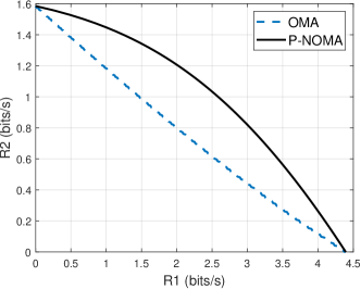
Figure 1: The achievable rate pairs in OMA and P-NOMA. The figure assumes that $(|h_{1}|^{2}/\sigma_{1}^{2})/(|h_{2}|^{2}/\sigma_{2}^{2})=10$, $P=2$, $W=1$, and that the powers $P_{i}$s, $i=1,2$, for OMA have been optimized to maximize the sum rate ($R_{1}+R_{2}$) for each given bandwidth split $\alpha_{\text{OMA}}$.

Let $\sigma_{r}^{2}$ denote the AWGN noise variance for user $r$. OMA splits the bandwidth $W$ between the two users such that user 1 communicates over allocated bandwidth $\alpha_{\text{OMA}}W$, and user 2 communicates over the allocated bandwidth $(1-\alpha_{\text{OMA}})W$. Let $P_{i}$ be the power allocated to user $i$, $i=1,2$, where $P_{1}+P_{2}=P$. Then, the achievable rates by OMA are given by:

$$R_{1}=\alpha_{\text{OMA}}W\log_{2}\Bigg{(}1+\dfrac{P_{1}|h_{1}|^{2}}{\alpha_{\text{OMA}}W\sigma_{1}^{2}}\Bigg{)},$$ (12)

$$R_{2}=(1-\alpha_{\text{OMA}})W\log_{2}\Bigg{(}1+\dfrac{P_{2}|h_{2}|^{2}}{(1-\alpha_{\text{OMA}})W\sigma_{2}^{2}}\Bigg{)}.$$ (13)

In comparison, for the P-NOMA system, we assume that the users’ channel qualities have been sorted such that $|h_{s}|^{2}/\sigma_{s}^{2}>|h_{w}|^{2}/\sigma_{w}^{2}$, where the subscripts $s$ and $w$ denote the stronger and weaker users, respectively. In the P-NOMA system, the stronger user can correctly decode their message as well as the weaker user’s message. However, the weaker user considers the stronger user’s message as noise for decoding [1]. Let $W$ denote the bandwidth of $p(t)$. For the raised cosine pulse, $W=(1/(2T))(1+\beta)$, where $\beta$ is the roll-off factor. Hence, the instantaneous achievable rates for the P-NOMA users are given by [5, 9]:

$$R_{s}=W\log_{2}\Bigg{(}1+\dfrac{P_{s}|h_{s}|^{2}}{W\sigma_{s}^{2}}\Bigg{)},$$ (14)

$$R_{w}=W\log_{2}\Bigg{(}1+\dfrac{P_{w}|h_{w}|^{2}}{P_{s}|h_{w}|^{2}+W\sigma_{w}^{2}}\Bigg{)},$$ (15)

where $P_{s}+P_{w}=P$. Fig. 1 compares the achievable rate pairs for OMA and P-NOMA. P-NOMA achieves strictly higher rates than OMA, except for the corner points where the base station communicates with only one user.

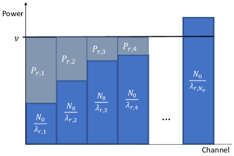
Figure 2: The water-filling algorithm finds the power level $\nu$ satisfying the power constraint. If $\inf\lambda_{r,n}>0$, then the water-filling solution gives that all allocated powers should satisfy $P_{r,n}\lambda_{r,n}=c$.

In contrast, in T-NOMA, the SVD baseline can decouple the superposition channel into $KN$ channels, where $K=2$ for the two-user channel. Hence, the achievable rate for user $r$ is given by [5]:

$$R_{r}=\dfrac{W}{KN}\sum_{n=1}^{N}\log_{2}\Bigg{(}1+\dfrac{P_{r,n}\lambda_{r,n}|h_{r}|^{2}}{(W/K)\sigma_{r}^{2}}\Bigg{)}.$$ (16)

It can be shown using the water filling algorithm that the average rate $R_{r}$ is maximized when all sub-channels have equal effective SNRs as illustrated in Fig. 2 (cf. [7]). Hence, the allocated powers $P_{r,n}$s depend on $\lambda_{r,n}$s such that $P_{r,n}\lambda_{r,n}=c$, where $c$ is a positive constant, subject to the power budget $\sum_{r,n}P_{r,n}=NP$. Thus, we have that $c=(NP)/(\sum_{r,n}1/\lambda_{r,n})$.

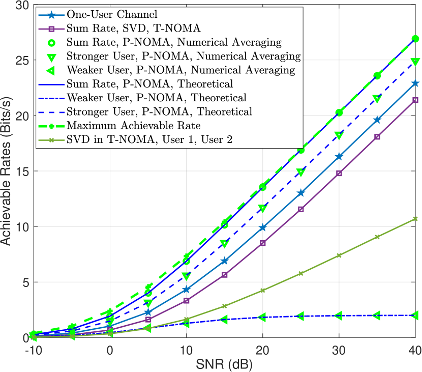
(a) $\beta=1$.

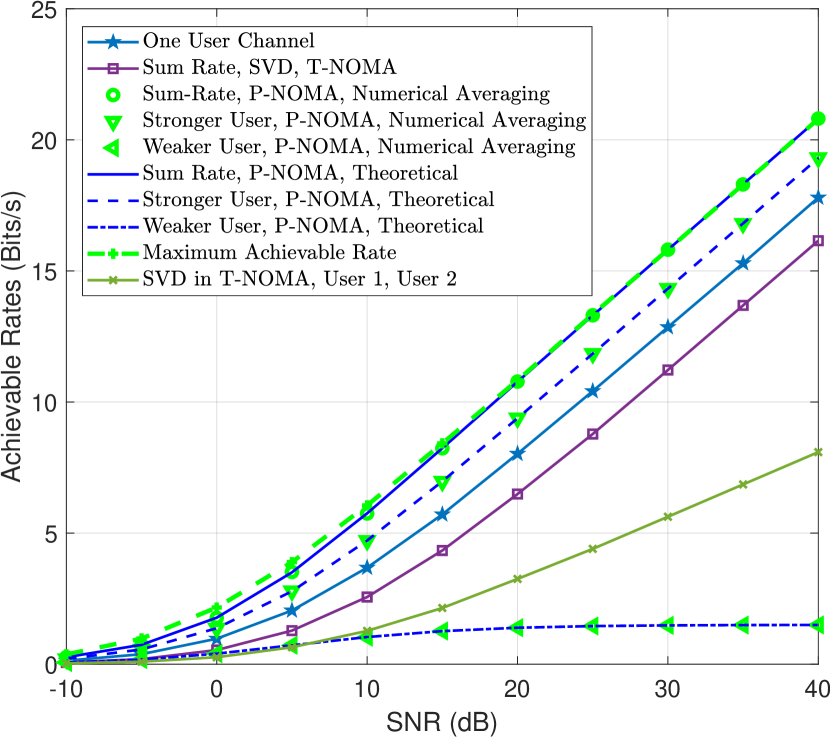
(b) $\beta=1/2$.

Figure 3: Achievable rates on the Rayleigh fading channel.

Fig. 3 compares the average achievable rates of P-NOMA and T-NOMA for two-user NOMA for different values of $\beta$. The derivation of the theoretical achievable rate curves for P-NOMA shown in Fig. 3 is presented in Appendix C. Numerical averaging indicates that rate expressions are averaged over many realizations of the channel fading coefficients. We assume that $\sigma_{1}^{2}=\sigma_{2}^{2}=N_{0}$. The average SNR per use is defined as $P/(2N_{0})$ for a fair comparison with the one-user system with power $P_{1}$. We set $P_{1}=P_{2}=1$, and $h_{r}\sim\mathcal{CN}(0,1)$. For T-NOMA, we use an offset $\tau=T/2$, which is the optimal offset for two-user T-NOMA [22, 10].

In P-NOMA, the achievable rate of the stronger user is much higher than the rate of the weaker user. The higher average-rate in P-NOMA for the stronger user comes at the cost of unfair channel usage, whereas T-NOMA aims at providing a high average rate while maintaining fairness among users. Furthermore, in P-NOMA, the achievable rate of the weaker user saturates at about 0.5 bits per channel use, whereas the individual rates for the SVD with T-NOMA do not, since both users achieve the same average rate. The SVD in T-NOMA achieves a lower sum rate than P-NOMA. In the SVD in T-NOMA, both users are allocated the same power and experience the same fading statistics. Hence, both users achieve the same achievable rate.

As shown in [9, 3], the channel capacity for T-NOMA is equivalent to the channel capacity for P-NOMA. Accordingly, the difference between SVD’s T-NOMA achievable rates and the maximum achievable rates (P-NOMA) suggests that encoding and decoding schemes can be developed that exceed the SVD method in T-NOMA. However, the design of such schemes can be difficult. Thus, we propose a data-driven AE that learns the encoding and decoding for T-NOMA. Although deriving closed-form achievable rates of CNN AE T-NOMA systems is an open problem, the CNN AE achieves much lower BERs than the SVD, as shown in Fig. 7 in Section V, which indicates higher achievable rates of the CNN AE than SVD’s achievable rates. We also provide an analysis of the average BER for P-NOMA in Appendix D. We discuss the BER performance in Section V.

IV Proposed AE for T-NOMA

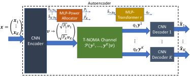
Figure 4: CNN autoencoder system. The encoder encodes the messages $\mathbf{x}$ for transmission as $\mathbf{v}$. The stochastic T-NOMA channel superimposes the transmitted sequences and uses faster than Nyquist signaling. The decoder at each user recovers the transmitted messages from the received sequence.

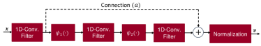
Figure 5: CNN encoder block diagram. The non-linear activation functions $\psi_{i}$s enable non-linear encoding. The final layer normalizes the output to satisfy the rate and power constraints.

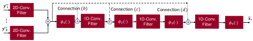
Figure 6: CNN decoder block diagram for user $r$. The first convolutional layer accepts the complex sequences of sufficient statistics for 2D-processing. The outcome sequence is further processed by 1D convolutional layers and non-linear activations.

IV-A AE Architecture

We propose a CNN-based AE for efficient encoding and decoding for T-NOMA. The CNN AE is shown in Fig. 4. At the transmitter, the encoder accepts the input message sequence $\mathbf{x}$ for transmission formed by concatenating the sequences of each user into a vector, i.e., $\mathbf{x}=[\mathbf{x}_{1}^{T},\ldots,\mathbf{x}_{K}^{T}]^{T}$, where $\mathbf{x}_{k}$ is an $N\times 1$ sequence intended for user $k$, $k=1,\ldots,K$. The CNN encoder encodes $\mathbf{x}$ into $\mathbf{v}$ for transmission, where $\mathbf{v}=[\mathbf{v}_{1}^{T},\ldots,\mathbf{v}_{K}^{T}]^{T}$, and $\mathbf{v}_{k}$ is the encoded sequence for user $k$. The encoded sequence $\mathbf{v}$ satisfies rate and power constraints. The encoding rate is one, which is the same rate as the baseline SVD method, i.e., both $\mathbf{x}$ and $\mathbf{v}$ are length-$KN$ sequences. The encoded sequence $\mathbf{v}$ passes through the T-NOMA channel as given in (4), with $v_{k}[n]$ replacing $x_{k}[n]$ in (5).

At the receiver, each user receives a sequence of sufficient statistics $\mathbf{y}^{r}=[\mathbf{y}^{rT}_{1},\ldots,\mathbf{y}^{rT}_{K}]^{T}$, as discussed in subsection II-A. At each user, a CNN decoder estimates the transmitted symbols from the received sequence to give $\hat{\mathbf{x}}_{k}$ for user $k$. During the training stage, the transmitted sequences and their estimates are used to compute the objective function. The encoder and decoder are jointly trained to minimize the objective function.

Encoder Architecture: The encoder block diagram is shown in Fig. 5. The CNN encoder consists of three finite impulse response (FIR) convolutional filter banks, two non-linear activations, and a normalization stage. The number of filters in each filter bank is denoted by $L_{e,i}$, $i=1,\ldots,U_{e}$, where $U_{e}$ is the number of convolutional stages at the encoder; $U_{e}$ = 3 in Fig. 5. The length of the filters in stage $i$ is denoted by $S_{e,i}$. After each of the first two convolutional stages, a non-linear activation $\psi_{i}(\cdot)$ is applied to the output. As a result of numerous experiments with different combinations of non-linear activations, we have concluded that the scaled exponential linear unit (SELU) is the most appropriate option for $\psi_{i}(\cdot)$. SELUs provide self-normalizing properties during training, thereby causing the hidden outputs to have zero mean and unit variance, which ameliorates vanishing or exploding gradients [23]. The SELU activation is defined by the element-wise operation:

$$\text{selu}(x)=\gamma\begin{cases}x,&\text{ if }x>0,\\ \alpha(e^{x}-1),&\text{ if }x\leq 0,\end{cases}$$ (17)

where $\gamma\approx 1.0507$ and $\alpha\approx 1.6732$. In addition to the non-linear activation, we also use batch normalization to reduce training performance sensitivity to weight initialization, while enabling some regularization benefits [24]. To ensure the output $\mathbf{v}$ has the expected length of $KN$ estimates, the hidden output samples can be padded with a few zero samples. The final layer is a normalization layer to ensure the transmitted symbols sequence is zero-mean and satisfies the power constraint $P_{k}=\dfrac{1}{N}\sum_{n=1}^{N}|v_{k}[n]|^{2}$. Moreover, we investigate the impact of the linear connection labeled (a) in the Fig. 5, which provides a more direct path for gradients to flow from the last convolutional layer to the first convolutional layer.

MLP Power allocator: Different from the SVD method, the AE does not necessarily decouple the users’ channels. Hence, water-filling or equal power allocation between channels is suboptimal for the AE. To leverage the end-to-end optimization of the AE for power allocation, we propose using a multilayer perceptron (MLP) power allocator (MLP-PA) that is jointly trained with the encoder and decoder. The MLP-PA accepts the estimates of the CSI at the transmitter for each user $\hat{h}_{r,\text{Tx}}$ to allocate the the available power to the sequences intended for each user, as shown in Fig. 4. We use two hidden layers for the MLP-PA. The first layer (input layer) is a size $2K\times M_{h_{1}}$ matrix that accepts the real and imaginary parts of the $K$ CSI terms and outputs $M_{h_{1}}$ hidden outputs. The hidden outputs are then passed through the selu($x$) activation. The first hidden layer contains a matrix of size $M_{h_{1}}\times M_{h_{2}}$ followed by selu($x$) activation. Batch normalization is used after the selu($x$) activation. The second hidden layer contains a matrix of size $M_{h_{2}}\times M_{h_{3}}$. The final layer linearly maps the $M_{h_{3}}$ outputs to $K$ outputs, denoted $o_{k}$. The matrix coefficients of the input and hidden layers are trainable parameters that are optimized in the end-to-end training process. The soft-max activation is applied to the $K$ hidden outputs to give the ratios of the total powers $P$ that will be allocated to the users. That is, the power allocated to user $k$ is computed as $P_{k}=Pe^{o_{k}}/\sum_{j=1}^{K}e^{o_{j}}$.

MLP CSI Combiner: Given the CSI estimate $\hat{h}_{r,\text{Rx}}$ at each user, the received signal is multiplied by $\hat{h}_{r,\text{Rx}}^{*}/|\hat{h}_{r,\text{Rx}}|^{2}$, which maximizes the SNR for linear combining [25]. Ideally, this multiplication cancels out the phase shift due to the fading channel when the CSI is known at the receiver. This strategy is optimal in a local sense, assuming that there is minimal or no IUI remaining in the received signals. We propose using an MLP CSI transformer (MLP-T) at each user that is optimized based on the end-to-end performance. MLP-T uses the CSI estimate $\hat{h}_{r,\text{Rx}}$ at each user to provide the combining factor $q_{r}$ as shown in Fig. 4 for user $r$. The MLP-T consists of two hidden layers with selu($x$) activation. The first layer accepts the real and imaginary parts of $\hat{h}_{r,\text{Rx}}$. This first layer contains a matrix of size $2\times M_{c_{1}}$. The second layer contains a matrix of size $M_{c_{1}}\times M_{c_{2}}$. Let $q_{r}$ denote the MLP-T combining factor at user $r$. Then, the output layer consists of a matrix that maps the $M_{c_{2}}$ hidden outputs to $[\operatorname{Re}\{q_{r}\},\operatorname{Im}\{q_{r}\}]$.

Decoder Architecture: Fig. 6 shows the CNN decoder’s architecture for detecting user $r$’s sequence $\mathbf{x}_{r}$. The input to the decoder is the sequence $\mathbf{y}^{r}$ scaled by the ratio combining factor $q_{r}$ to give $\mathbf{y}^{\prime r}\triangleq q_{r}\mathbf{y}^{r}$. Let the number of filters at each convolutional stage be denoted by $L_{d,i}$, and the length of filters at each stage be denoted by $S_{d,i}$, where $i=1,\ldots,U_{d}$, and $U_{d}$ is the number of convolutional stages at the decoder; $U_{d}=4$ in Fig. 6. The first convolutional layer uses 2D FIR filters to process the real and imaginary parts of $\mathbf{y}^{\prime r}_{l}$. The 2D convolution produces 1D-sequences for each 2D filter bank for further processing. The output 1D-sequences per 2D filter bank are then summed to give 1D sequences. Then, a non-linear activation $\phi_{1}(\cdot)$ is applied followed by 1D-convolutional layers and non-linear activations. The SELU is selected as the non-linear activation for $\phi_{1}(\cdot)$ and $\phi_{2}(\cdot)$. For $\phi_{3}(\cdot)$, the hard swish (h-swish) function is used [26]. Batch normalization is applied at the output of $\phi_{i}(\cdot)$, $i=1,2,3$. The output of the final convolutional layer is passed through a final activation $\phi_{4}(\cdot)$ to give the estimate $\hat{\mathbf{x}}_{r}$ of the length-$N$ symbols sequence intended for user $r$. The activation $\phi_{4}(\cdot)$ depends on the training criteria as discussed in subsection IV-B.

IV-B Training Criteria

Cross-entropy: Sequence detection can be formulated as a multi-class multi-label classification problem (cf. [27]). Let $\mathds{1}_{x[n]=m}$ denote the indicator function such that $\mathds{1}_{x[n]=m}=1$ if $x[n]=m$ (and zero otherwise), where $m=0,1,\ldots,M-1$, $M$ is the cardinality of the message set for $x[n]$, and $p_{m,n}=\Pr\{x[n]=m\}$ be the soft estimate $\hat{x}[n]$. Then, the CE loss $\mathcal{H}\{x[n],\hat{x}[n]\}$ between the estimate and the correct message is given by:

$$\mathcal{H}\{x[n],\hat{x}[n]\}=-\sum_{m=0}^{M-1}\mathds{1}_{x[n]=m}\log(p_{m,n}).$$ (18)

Consider the $i$th input sequence $\mathbf{x}^{\langle i\rangle}$ in a training mini-batch, $i=0,\ldots,L-1$, where $L$ is the number of input sequences in a mini-batch. Then, the average CE loss $J_{\text{CE}}$ is computed by averaging the CE loss over the sequences in the mini-batch as follows:

$$J_{\text{CE}}=\dfrac{1}{LKN}\sum_{i=0}^{L-1}\sum_{n=0}^{KN-1}\mathcal{H}\{x^{\langle i\rangle}[n],\hat{x}^{\langle i\rangle}[n]\}.$$ (19)

If $M=2$, then $\phi_{4}(\cdot)$ can be the sigmoid activation $\text{sigmoid}(x)=1/(1+e^{-x})$, where the output of the final convolutional layer has length $N$. In this case, the output of the CNN is $p_{0,n}$, $0\leq n\leq N$. If $M>2$, then $\phi_{4}(\cdot)$ is the soft-max activation $\sigma(\mathbf{z}_{n})_{m}=e^{z_{n,m}}/\sum_{m=0}^{M-1}e^{z_{n,m}}$, where the last convolutional layer produces $M$ output sequences $\mathbf{z}=[\mathbf{z}_{n}]$ such that $\mathbf{z}_{n}=[z_{0,n},\ldots,z_{M-1,n}]$. MSE: The MSE can be used for training the AE. For MSE training, $\phi_{4}(\cdot)$ can be the identity function $I(x)=x$. Then, the output is the estimate of the message in the Euclidean distance sense (as opposed to the probability of correct bit estimation in CE training). The sample average squared error $J_{\text{MSE}}$ over the entire sequence in a mini-batch is computed as follows:

$$J_{\text{MSE}}=\dfrac{1}{LKN}\sum_{i=0}^{L-1}\sum_{n=0}^{KN-1}(x^{\langle i\rangle}[n]-\hat{x}^{\langle i\rangle}[n])^{2}.$$ (20)

In the case where $M=2$, the tanh activation can also be used for $\phi_{4}(\cdot)$ instead of $I(x)$.

Cross-entropy with Q-function In comparison with the MSE loss, the cross-entropy loss has been shown to produce lower BERs. Nevertheless, achieving the minimum cross-entropy does not guarantee achieving the minimum BER. We use the first and second order statistics of the LLRs in each mini-batch to further decrease the BER during training. Assume the transmitted symbols follow the BPSK modulation. The LLR is defined as:

$$\text{LLR}_{i} =\log\Big{(}\dfrac{\Pr\{x_{i}=+1\}}{\Pr\{x_{i}=-1\}}\Big{)}=\log\Big{(}\dfrac{\hat{p}_{i}}{1-\hat{p}_{i}}\Big{)}.$$ (21)

For each mini-batch, assume the LLRs are Gaussian. Our goal is to minimize the overlap between the Gaussian corresponding to a $+1$ transmitted bit and the Gaussian corresponding to a $-1$ transmitted bit. This overlap is captured by the Q-function, where $Q(x)\triangleq(1/\sqrt{2\pi})\int_{x}^{\infty}e^{-u^{2}/2}du$.

In a mini-batch containing $L$ sequences of length-$N$ bits per user, we compute the means and variances of the conditional LLRs. Let $s\in\{-1,+1\}$ denote the transmitted symbol. Each mini-batch contains $L_{s}+N_{s}$ LLRs corresponding to symbol $s$, where $L_{+1}+L_{-1}=L$, and $N_{+1}+N_{-1}=N$. Let LLR${}^{s}_{a,b}$ denote the conditional LLRs corresponding to symbol $s$, where $a=0,\ldots,L_{s}-1$, and $b=0,\ldots,N_{s}-1$. Then, the empirical mean and variance of LLR${}^{s}_{a,b}$ are computed as follows:

$$\mu_{s}=\dfrac{1}{L_{s}N_{s}}\sum_{a,b}\text{LLR}^{s}_{a,b},\text{ and }\sigma^{2}_{s}=\dfrac{1}{L_{s}N_{s}}\sum_{a,b}(\text{LLR}^{s}_{a,b}-\mu^{s})^{2}.$$ (22)

We introduce the training Q-function loss (Q-loss) as:

$$J_{\text{Q}}\triangleq\dfrac{1}{2}\sum_{s}Q\bigg{(}\gamma\dfrac{\mu_{s}}{\sigma_{s}}\bigg{)},$$ (23)

where $\gamma>0$ is a hyperparameter to be tuned. The combined cross-entropy with Q-loss objective function is given by:

$$J_{\text{CEQ}}=\mathcal{H}\{x[n],\hat{x}[n]\}+\alpha J_{\text{Q}},$$ (24)

where $\alpha>0$ is the weight factor. Empirically, we find that small values of $\alpha$ in the range $(0,1)$ can provide significant BER improvements for appropriate values of $\gamma$. The Q-loss in (23) can be extended to $M$-QAM and $M$-PSK modulations by defining $M$-ary LLRs (cf. [28]).

Table I: Number of convolutional filters $L_{e,i}$ and $L_{d,j}$ for the encoders and decoders of different variants of the CNN AE, $i=1,2,3$ and $j=1,2,3,4$. All CNN AEs user FIR filters of length 11 samples, i.e., $S_{e,i}=S_{d,j}=11$.

Method	Encoder	Decoder
CNN AE1	$1,1,1$	$1,1,1,1$
CNN AE2	$2,4,2$	$1,1,1,1$
CNN AE3	$2,4,2$	$1,1,2,2$
CNN AE4	$1,1,1$	$2,4,4,2$
CNN AE5	$2,4,2$	$2,4,4,2$
CNN AE6	$1,1,1$	$1,2,8,4$
CNN AE7	$1,1,1$	$2,16,128,16$
CNN AE8	$2,4,2$	$2,16,128,16$
CNN AE9	$2,4,2$	$4,32,128,16$

IV-C Complexity Comparison

Table II: Complexity comparison for sequence estimation. The numerical values give the complexity order for the simulated system with $K=2$ and $N=512$, and CNN AE5. The CNN AE also requires $O(KN)$ and $O(K^{3}N)$ computations of the non-linear activations for the encoder and decoder, respectively. For MLP-PA we use $M_{h_{i}}=32$. For MLP-T, we use $M_{c_{i}}=8$.

Method	FLOPs	Storage
SVD, Encoder	$(KN)^{2}$ $\sim 1.0486\times 10^{6}$	$(KN)^{2}$ $\sim 1.0486\times 10^{6}$
SVD, Decoder	$(KN)^{2}$ $\sim 1.0486\times 10^{6}$	$(KN)^{2}$ $\sim 1.0486\times 10^{6}$
CNN AE, Encoder	$KN\sum_{i=1}^{U_{e}}L_{e,i}S_{e,i}$ $\sim 1.8022\times 10^{5}$	$K\sum_{i=1}^{U_{e}}L_{e,i}S_{e,i}$ $\sim 352$
CNN AE, Decoder	$K^{2}N(2KL_{d,1}S_{d,1}+\sum_{i=2}^{U_{d}}L_{d,i}S_{d,i})$ $\sim 4.0550\times 10^{5}$	$K(2KL_{d,1}S_{d,1}+\sum_{i=2}^{U_{d}}L_{d,i}S_{d,i})$ $\sim 396$
MLP-PA	$M_{h_{1}}(2K+M_{h_{2}})+M_{h_{2}}M_{h_{3}}+M_{h_{3}}\sim 656$	$M_{h_{1}}(2K+M_{h_{2}})+M_{h_{2}}M_{h_{3}}+M_{h_{3}}\sim 656$
MLP-T	$2M_{c_{1}}+M_{c_{1}}M_{c_{2}}+2M_{c_{2}}\sim 96$	$2M_{c_{1}}+M_{c_{1}}M_{c_{2}}+2M_{c_{2}}\sim 96$

Table II summarizes the complexity and storage requirements for the SVD-based baseline and the CNN AE employed in the T-NOMA system. The baseline pre-multiplies the $KN\times 1$ vector $\mathbf{Px}$ by a $KN\times KN$ matrix and post-multiples the received signal sequence $\mathbf{y}^{r}$ by another $KN\times KN$ matrix. Hence, the order of the number of floating-point operations (FLOPs), i.e., elementary multipliers and adders, for each matrix multiplication is $O(KN)^{2}$ per sequence encoding and decoding. Whereas, the CNN AE uses discrete-time convolutions, which require $O(KNL_{e,i}S_{e,i})$ and $O(K^{2}N{L_{d,i}S_{d,i}})$ FLOPs for each convolutional layer in the encoder and the decoder, respectively. Therefore, the CNN AE’s complexity is linear in $N$, whereas the SVD’s complexity is quadratic in $N$.

Furthermore, the SVD method stores $(KN)^{2}$ parameters at the encoder and decoders. In contrast, the CNN AE only stores the coefficients of the FIR filters at each convolutional stage and the batch normalization means and variances, which gives a storage order of $KL_{e,i}S_{e,i}$ and $K^{2}L_{d,1}S_{d,1}$ for the encoder and decoder respectively. For the CNN decoder, where $K$ is large, the complexity is dictated by the first convolutional layer because it processes the length-$KN$ complex sequence of sufficient statistics. Thus, compared with the SVD’s quadratic storage order in $KN$, the CNN AE’s storage is independent of $N$ and quadratic in $K$.

V Numerical Results

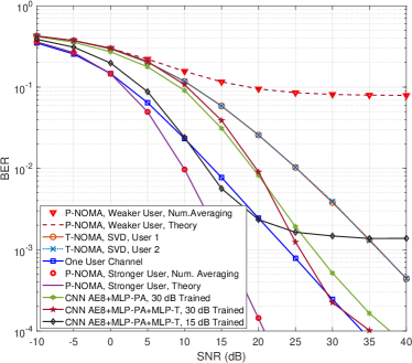
Figure 7: BER comparison between P-NOMA, T-NOMA, and a one-user Rayleigh fading channel. P-NOMA allows reliable transmission only for the stronger user. In contrast, T-NOMA allows two users to communicate reliably by sharing the same orthogonal resource element, while guaranteeing fairness among users. The CNN AE BER curves are identical for both users. Hence, given the same average SNR per user, the CNN AE8 communicates at double the rate of a single-user system while maintaining the same BER when trained at SNRs of 15 dB and 30 dB.

We present simulation results to compare the BER performances of the discussed systems. We consider a two-user NOMA system, i.e., $K=2$, with binary phase shift keying (BPSK) modulation for both users. The fading is Rayleigh distributed such that $\mathbf{E}\{|h_{i}|^{2}\}=1$, $i=1,2$. Also, both users have the same variance of the AWGN electronics noise, i.e., $\sigma_{1}^{2}=\sigma_{2}^{2}=N_{0}$. The SNR is computed with respect to user 1’s signal, i.e., SNR $=\mathbf{E}\{|h_{1}|^{2}/\sigma_{1}^{2}\}=1/N_{0}$. We set the frame length as $N=512$ data symbols per user. Testing is performed using $64\times 2048=131,072$ frames. We use the root raised cosine pulse (RRCP) with a unity roll-off factor for $p(t)$. The discrete time raised cosine pulse (RCP) samples $\mathbf{g}_{l,k}$ are sampled accordingly and truncated to have an ISI span of 7 symbols per user, which captures most of the energy in the RCP. For T-NOMA, we use the timing offset $\tau_{\text{design}}=T/2$, which is the optimal offset for two-user NOMA [22]. The allocated powers $P_{r,n}$s depend on $\lambda_{r,n}$s such that $P_{r,n}\lambda_{r,n}=c$, where $0<c<1$, subject to the power budget $\sum_{r,n}P_{r,n}=NP$, where $P=2$. The average BER results with BPSK modulation for P-NOMA are obtained by numerically averaging $\text{BER}_{i}=Q(\sqrt{2\eta_{i}})$ for several random realizations of the instantaneous channel SNRs $\eta_{i}$, where $i\in\{s,w\}$ corresponds to the stronger user and the weaker user, respectively, and $Q(.)$ denotes the Gaussian $Q$-function. Moreover, we use $\eta_{s}=P_{s}|h_{s}|^{2}/(WN_{0})$ and $\eta_{w}=(P_{w}|h_{w}|^{2})/(P_{s}|h_{w}|^{2}+WN_{0})$, where the channel gains have been sorted such that $|h_{s}|^{2}/\sigma_{s}^{2}>|h_{w}|^{2}/\sigma_{w}^{2}$,. The theoretical BER curves for P-NOMA are obtained by using (54) and (55) in Appendix D. For all T-NOMA results, we simulate a T-NOMA system as discussed in subsection II-A.

Table III: Hyperparameters Settings.

Hyperparameter	Setting
Number of Data Symbols per Sequence per User	$512$
Number of Training Sequences	$131,072$
Number of Validation Sequences	$512$
Number of Testing Sequences	$131,072$
Number of Sequences per Training Minibatch	$32$
Learning Rate	$3\times 10^{-3}$
Number of Training Epochs	$20$
Training Algorithm	Adam
Training SNR	$30$ dB
Design Time Offset	$T/2$
Number of Users	$2$
Fading Distribution	Rayleigh
Distribution of Timing Error	Uniform
Distribution of CSI Error	Gaussian

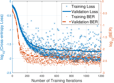
Figure 8: Learning curve.

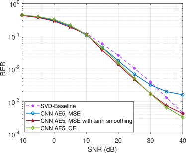
Figure 9: BER performance comparison between the SVD baseline and the CNN AE with different training modes.

V-A BER Performance in P-NOMA vs. T-NOMA

This subsection investigates the bit error rate (BER) performance of P-NOMA and T-NOMA systems in the absence of timing or CSI estimation errors. Fig. 7 illustrates a comparison of BER performance between P-NOMA and T-NOMA systems.

In P-NOMA, while the stronger user attains the best BER results, the weaker user’s performance shows an error floor, plateauing at approximately 0.08 BER by 20 dB. On the other hand, T-NOMA, using the SVD method, provides equal BER performance for both users, ensuring fairness. Additionally, the average BER for P-NOMA levels off at around 20 dB due to the weaker user’s significantly higher BER. In contrast, T-NOMA exhibits a consistent decline in BER for both users as the signal-to-noise ratio (SNR) increases. By 20 dB SNR, T-NOMA outperforms P-NOMA in terms of average user performance. Fig. 7 also includes the BER performance of a single-user system with maximum likelihood (ML) detection over the Rayleigh fading channel.

At an SNR of 30 dB, the convolutional neural network (CNN) AE8 with the multilayer perceptron power allocation (MLP-PA) surpasses the SVD performance by around 9 dB. When the MLP-T is incorporated into the CNN AE8, an additional 3 dB improvement in performance is observed. When trained at 15 dB, the CNN AE system demonstrates significant gains over the SVD for SNRs ranging from 5 dB to 30 dB. Given the same average SNR per user, the CNN AE8 communicates at double the rate of a single-user system while maintaining the same BER when trained at SNRs of 15 dB and 30 dB.

V-B SVD-baseline vs. CNN AE for T-NOMA

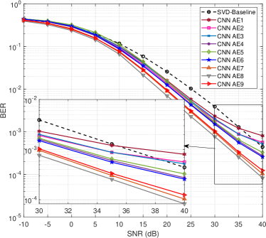
Figure 10: BER performances for several CNN AE variants. The complexity increases from CNN AE1 to CNN AE9.

We compare the BER performances of the CNN AE and the SVD in T-NOMA. The CNN AE is trained using randomly generated $131,072$ frames at 30 dB SNR and tested using another random set of $131,072$ frames per testing SNR, where each frame contains 512 bits per user. The Adam optimizer, a variant of the stochastic gradient descent algorithm, is used in the back propagation [29]. The CNN AE is trained for 20 epochs using a fixed base learning rate of $3\times 10^{-3}$. The CNN AE system is implemented in Python using the Pytorch library. Table III summarizes the settings used in the simulations. Fig 8 shows the progressions of the BER and the CE with training iterations. Minimizing the CE coincides with reducing the BER.

Initially, we consider the scenario without timing or CSI estimation errors. The CNN AE includes the encoder and decoder CNNs, excluding the MLP components unless specified. The default power allocation for the CNN AE is $P_{1}=P_{2}=1$ unless otherwise stated. Fig. 9 compares the BER performances of the SVD method and the CNN AE5 for the T-NOMA system. Using CE training, the CNN AE outperforms the SVD for SNRs larger than 10 dB. For SNRs between 20 dB and 35 dB, the CNN AE achieves between 2 dB and 3 dB SNR gains over the SVD.

Additionally, CE training of the CNN AE yields better performance than MSE training. The performance under MSE training improves when utilizing a tanh activation function for output smoothing. In some scenarios, MSE is easier to compute than CE. Therefore, in such cases, tanh smoothing enables the achievement of BERs comparable to those obtained through CE training.

V-C BER Performance of Different Variants of the CNN AE

This subsection illustrates the performance-complexity trade-off of the CNN AE where no timing or CSI errors are present. Fig. 10 shows the BER performances of the different CNN AE variants shown in Table I. CNN AE1 uses the fewest number of filters in our proposed architecture and requires the lowest complexity. CNN AE9 entails the highest computational complexity among the variants. Interestingly, CNN AE4 uses fewer filters at the encoder than CNN AE5 and achieves similar BER performance. This suggests that increasing the decoder’s complexity can yield higher performance improvements than increasing the encoder’s complexity. The best performance is achieved by CNN AE8, which outperforms the SVD by about 8 dB at an SNR of 30 dB. We note that with further tuning of the hyperparameters using Bayesian optimization (cf. [30]), CNN AE9 may perform at least as well as CNN AE8.

V-D Benefits of Q-function Loss

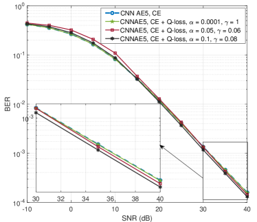
Figure 11: Impact of Q-function loss.

Fig. 11 shows CNN AE5’s BER performance with different loss functions. By combining the CE with the Q-function loss, we achieve around 0.8 dB gain for a BER of $2\times 10^{-4}$. To achieve this gain, the hyperparameters $\alpha$ and $\gamma$ must be tuned appropriately. The BER gain can be achieved at no increase in inference complexity, at the cost of using the combined CE and Q-function loss during training.

V-E Benefits of Linear Connections

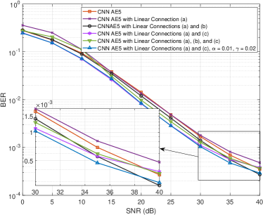
Figure 12: Impact of linear connections.

Fig. 12 illustrates the BER performance of CNN AE5 with different linear connections combinations at the encoder and decoder. We note that including linear connections (a) and (c) provides around 2.2 dB gain for a BER of $1.1\times 10^{-3}$ compared with a CNN AE5. With the CNN AE5 architecture, including linear connections (a) and (c) results in best performance at the training SNR of 30 dB, but connections (a) and (b) provide the best performance at 40 dB SNR, with crossover occurring at about 35 dB. When the combined CE and Q-function loss is used for training, the gain over the best performing system trained only with CE is between 0.5 dB and 1 dB for SNRs between 30 dB and 38 dB.

V-F Impact of Imperfect CSI

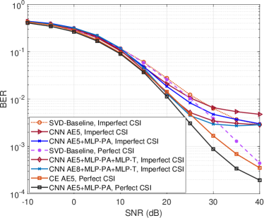
Figure 13: Impact of imperfect CSI on BER performance. The error on the CSI is added at 20 dB, i.e., $\mathbf{E}[|\delta|^{2}]=0.01$.

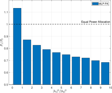
Figure 14: Power allocation using MLP power allocator for different realizations of the CSI.

This subsection investigates the impact of imperfect CSI at the transceivers on the BER of the SVD and the CNN AE when no timing errors are present. Fig. 13 shows the impact of imperfect CSI on the performances of the SVD and the CNN AE. Imperfect CSI causes error floors in the BERs of all methods. The reason is that the error on the CSI estimate not only results in data dependent noise, but also affects the AWGN as shown in (11). The MLP-PA improves the resilience of the CNN AE to imperfect CSI. Furthermore, including the MLP-T allows further performance gains by the CNN system. For SNRs between 20 dB and 30 dB, CNN AE5 with the MLP-PA and the MLP-T provide up to 7 dB gain in performance over the SVD baseline. Fig. 14 shows a histogram of the power allocation between users by the MLP-PA. The MLP-PA allocates power according to the end-to-end CE of the system. Fig. 14 shows that allocating more power to the weaker user enables improvement in the end-to-end BER.

V-G Impact of Timing Offset Error

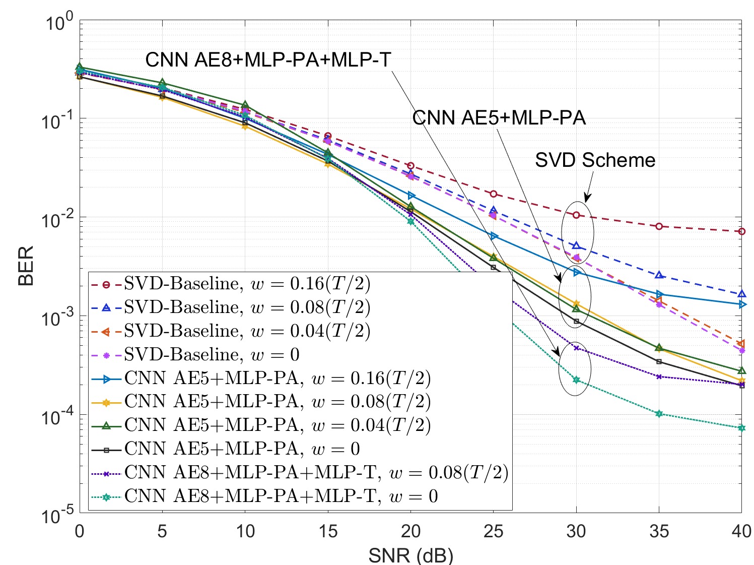
Figure 15: Impact of imperfect timing offset error on the BER performance. The timing error is added at width of $w\times$ the design offset $\tau_{\text{design}}$, i.e., $\epsilon\sim U(-(w/2)\tau_{\text{design}},(w/2)\tau_{\text{design}})$.

This subsection considers the impact of timing error on the BER performance, where perfect CSI is assumed. Fig. 15 shows the impact of timing error on the performance of SVD baseline and CNN AE5 with MLP-PA. Timing errors cause about 5 dB loss in performance for the SVD. In contrast, CNN AE5 experiences about a 2 dB loss in performance at high SNRs. CNN AE5 outperforms the SVD baseline by significant margins at high SNRs when timing error is introduced to the NOMA system, e.g., by about 10 dB at a BER of $2\times 10^{-3}$. Hence, the CNN AE is more robust to timing errors than the SVD method.

V-H Impact of Timing Error and Imperfect CSI

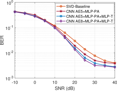
Figure 16: BER performance comparison between the SVD and the CNN AE where the CSI error variance is 0.01, and the timing error width is at $16\%$ of $\tau_{\text{design}}$.

This subsection considers the effect of both imperfect CSI and timing errors. Fig. 16 compares the BERs of CNN AE5 and the SVD method when both timing error and imperfect CSI are considered. CNN AE5 with the MLP-PA achieves about 2 dB gain in performance over the SVD for SNRs between 20 dB and 30 dB. Moreover, integrating the MLP-T with CNN AE5 achieves an additional 1 dB to 2 dB gains for SNRs between 20 dB and 40 dB. CNN AE8 achieves an additional 2 dB gain at an SNR of 25 dB. Both CNN AEs achieve approximately the same BER by an SNR of 40 dB. Also, at BERs of $4\times 10^{-3}$ and $3\times 10^{-3}$, CNN AE5 and CNN AE8 with MLP-PA and MLP-T achieve gains of 10 dB and greater than 10 dB over SVD, respectively.

VI Conclusion

We propose a convolutional neural network (CNN) auto-encoder (AE) for downlink time-offset with faster than Nyquist signaling non-orthogonal multiple access (T-NOMA). As in previous studies, our simulations demonstrate that T-NOMA satisfies the user fairness criterion, whereas P-NOMA does not. In T-NOMA, the singular value decomposition (SVD) baseline’s encoding and decoding complexities are quadratic in the length of the transmitted sequence. In comparison, the proposed AE’s encoding and decoding complexities are linear in the length of the transmitted sequence. Using simulated data of a two-user T-NOMA system, we have shown that the AE outperforms the SVD baseline by about 2 dB for BERs less than $10^{-2}$ under perfect CSI conditions. We have also shown that the CNN AE entails a linear time complexity in the length of the transmitted sequence, whereas the SVD entails a quadratic time complexity. We have proposed a multilayer perceptron (MLP) power allocator (MLP-PA) and an MLP transformer (MLP-T) for power allocation and channel state information (CSI) transformation that are trained using the end-to-end performance. the AE with MLP-PA outperforms the SVD baseline by about 6 dB at BERs of about $10^{-3}$. Furthermore, we have demonstrated that the CNN AE system can be more resilient to timing error and imperfect CSI than the SVD baseline. In addition, future works can study the impact of CSI errors and timing errors on the achievable rates.

Appendix A Sufficient Statistic Samples for Matched Filter Output in T-NOMA

Let $p(t)$ be the root raised cosine pulse. Assuming $P_{k,n}=1$, $h_{r}=1$, and no noise, then $y^{r}(t)$ is given by

$$y^{r}(t)=\sum_{n}x_{1}[n]p(t-T/2-(n-1)T)+\sum_{n}x_{2}[n]p(t-(n-1)T)$$ (25)

Then, the sufficient statistics sequence $[\mathbf{y}_{1}^{r},\mathbf{y}_{2}^{r}]$ is obtained as follows. The sequence $\mathbf{y}_{1}^{r}$ is obtained by correlating $y^{r}(t)$ with $p(t-(m-1)T-T/2)$. That is,

$$y_{1}^{r}[m]= \int_{-\infty}^{\infty}y^{r}(\lambda)p(\lambda-(m-1)T-T/2)d\lambda$$ (26)

$$= \sum_{n}x_{1}[n]\int_{-\infty}^{\infty}p(\lambda-T/2-(n-1)T)p(\lambda-(m-1)T-T/2)d\lambda$$

$$+\sum_{n}x_{2}[n]\int_{-\infty}^{\infty}p(\lambda-(n-1)T)p(\lambda-(m-1)T-T/2)d\lambda.$$ (27)

Using a change of variable $\lambda^{\prime}=\lambda-T/2-(n-1)T$ for the first integral, and a change of variable $\lambda^{\prime}=\lambda-(n-1)T$ for the second integral, we get

$$y_{1}^{r}[m]= \sum_{n}x_{1}[n]\int_{-\infty}^{\infty}p(\lambda^{\prime})p(\lambda^{\prime}+(n-m)T)d\lambda^{\prime}$$

$$+\sum_{n}x_{2}[n]\int_{-\infty}^{\infty}p(\lambda^{\prime})p(\lambda^{\prime}+(n-m)T-T/2)d\lambda^{\prime}$$ (28)

$$= \sum_{n}x_{1}[n]\int_{-\infty}^{\infty}p(\lambda^{\prime})p((m-n)T-\lambda^{\prime})d\lambda^{\prime}$$

$$+\sum_{n}x_{2}[n]\int_{-\infty}^{\infty}p(\lambda^{\prime})p((m-n)T+T/2-\lambda^{\prime})d\lambda^{\prime},$$ (29)

where the last equality follows by the even symmetry of $p(t)$. Thus,

$$y_{1}^{r}[m]=\sum_{n}x_{1}[n](p*p)(t)|_{t=(m-n)T}+\sum_{n}x_{2}[n](p*p)(t)|_{t=(m-n)T+T/2}.$$ (30)

The sequence $\mathbf{y}_{2}^{r}$ is obtained by correlating $y^{r}(t)$ with $p(t-(m-1)T)$. Hence,

$$y_{2}^{r}[m]= \int_{-\infty}^{\infty}y^{r}(\lambda)p(\lambda-(m-1)T)d\lambda$$ (31)

$$= \sum_{n}x_{1}[n]\int_{-\infty}^{\infty}p(\lambda-T/2-(n-1)T)p(\lambda-(m-1)T)d\lambda$$

$$+\sum_{n}x_{2}[n]\int_{-\infty}^{\infty}p(\lambda-(n-1)T)p(\lambda-(m-1)T)d\lambda.$$ (32)

Using a change of variable $\lambda^{\prime}=\lambda-T/2-(n-1)T$ for the first integral, and a change of variable of $\lambda^{\prime}=\lambda-(n-1)T$ for the second integral, we get

$$y_{2}^{r}[m]= \sum_{n}x_{1}[n]\int_{-\infty}^{\infty}p(\lambda^{\prime})p(\lambda^{\prime}+(n-m)T+T/2)d\lambda^{\prime}$$

$$+\sum_{n}x_{2}[n]\int_{-\infty}^{\infty}p(\lambda^{\prime})p(\lambda^{\prime}+(n-m)T)d\lambda^{\prime}$$ (33)

$$= \sum_{n}x_{1}[n]\int_{-\infty}^{\infty}p(\lambda^{\prime})p((m-n)T-T/2-\lambda^{\prime})d\lambda^{\prime}$$

$$+\sum_{n}x_{2}[n]\int_{-\infty}^{\infty}p(\lambda^{\prime})p((m-n)T-\lambda^{\prime})d\lambda^{\prime},$$ (34)

where the last equality follows by the even symmetry of $p(t)$. Thus, we get

$$y_{2}^{r}[m]=\sum_{n}x_{1}[n](p*p)(t)|_{t=(m-n)T-T/2}+\sum_{n}x_{2}[n](p*p)(t)|_{t=(m-n)T}.$$ (35)

Appendix B Average Rate analysis for P-NOMA with Two Users

For P-NOMA with two users, the users’ instantaneous SNRs have been sorted such that $|h_{s}|^{2}/\sigma_{s}^{2}>|h_{w}|^{2}/\sigma_{w}^{2}$. Therefore, the user associated to $\gamma_{s}=|h_{s}|^{2}/(W\sigma_{s}^{2})$ is considered as the stronger user and the user associated to $\gamma_{w}=|h_{w}|^{2}/(W\sigma_{w}^{2})$ is considered as the weaker user. We assume that the unsorted users’ SNRs $\alpha_{1}$ and $\alpha_{2}$ follow the Rayleigh fading distribution, such that, for $i=1,2$, the cumulative distribution function (CDF) of $\alpha_{i}\triangleq|h_{i}|^{2}/\sigma_{i}^{2}$ is given by $F_{\alpha_{i}}(y)=1-e^{-y/\overline{\alpha}_{i}}$, where $\overline{\alpha}_{i}$ is the average value of ${\alpha}_{i}$. Accordingly, we can easily show that for the stronger user with SNR $\gamma_{s}=\max\left(\alpha_{1},\alpha_{2}\right)$, its CDF expression can be expressed as $F_{\gamma_{s}}(y)=\prod_{i=1}^{2}F_{\alpha_{i}}(y)$, which can be written as $F_{\gamma_{s}}(y)=1-e^{-y/\overline{\alpha}_{1}}-e^{-y/\overline{\alpha}_{2}}+e^{-y(1/\overline{\alpha}_{1}+1/\overline{\alpha}_{2})}$. However, for the weaker user with SNR $\gamma_{w}=\min\left(\alpha_{1},\alpha_{2}\right)$, we can obtain the CDF expression as $F_{\gamma_{w}}(y)=1-\left[1-F_{\alpha_{1}}(y)\right]\left[1-F_{\alpha_{2}}(y)\right]=1-e^{-y(1/\overline{\alpha}_{1}+1/\overline{\alpha}_{2})}$.

The instantaneous achievable rate for the stronger and the weaker users can respectively be expressed as [5]:

$$R_{s} =W\log_{2}\left(1+\frac{P_{s}|h_{s}|^{2}}{W\sigma_{s}^{2}}\right),$$ (36)

$$R_{w} =W\log_{2}\left(1+\frac{P_{w}|h_{w}|^{2}}{P_{s}|h_{w}|^{2}+W\sigma_{w}^{2}}\right),$$ (37)

where $P_{s}$ and $P_{w}$ denote the allocated power to the stronger and weaker users, respectively, and $P=P_{s}+P_{w}$ is the total allocated power. Assuming that $X_{s}=\gamma_{s}\,P_{s}$, where $\gamma_{s}=|h_{s}|^{2}/(W\sigma_{s}^{2})$, the average rate for the stronger user $\overline{R}_{s}$ can be obtained by averaging $R_{s}$ using the probability density function (PDF) of $X_{s}$, $f_{X_{s}}(x_{s})$; hence, $\overline{R}_{s}$ can be written as a function of $F_{X_{s}}(x_{s})$ as:

$$\overline{R}_{s} =W\int_{0}^{\infty}\log_{2}\left(1+x_{s}\right)f_{X_{s}}(x_{s})\,d{x_{s}}=W\log_{2}(e)\int_{0}^{\infty}\frac{1-F_{X_{s}}(x_{s})}{1+x_{s}}\,d{x_{s}},$$ (38)

where the second equality follows by integration be parts. Since $F_{X_{s}}(x_{s})={\rm P}(X_{s}\leq x_{s})={\rm P}(\gamma_{s}\,P_{s}\leq x_{s})=F_{\gamma_{s}}(x_{s}/P_{s})$, then, $F_{X_{s}}(x_{s})=1-e^{-x_{s}/(P_{s}\overline{\alpha}_{1})}-e^{-x_{s}/(P_{s}\overline{\alpha}_{2})}+e^{-x_{s}(1/(P_{s}\overline{\alpha}_{1})+1/(P_{s}\overline{\alpha}_{2}))}$. Then, (38) becomes

$$\overline{R}_{s} =W\log_{2}(e)\int_{0}^{\infty}\frac{1}{1+x_{s}}\left[e^{-\frac{x_{s}}{P_{s}\overline{\alpha}_{1}}}+e^{-\frac{x_{s}}{P_{s}\overline{\alpha}_{2}}}-e^{-x_{s}(\frac{1}{P_{s}\overline{\alpha}_{1}}+\frac{1}{P_{s}\overline{\alpha}_{2}})}\right]\,d{x_{s}}.$$ (39)

The first integral in (39) can be evaluated as $\int_{0}^{\infty}\frac{1}{1+x_{s}}e^{-x_{s}/(P_{s}\overline{\alpha}_{1})}\,d{x_{s}}=\int_{1}^{\infty}\frac{1}{t}e^{-(t-1)/(P_{s}\overline{\alpha}_{1})}\,d{t}$ $=e^{1/(P_{s}\overline{\alpha}_{1})}\int_{1}^{\infty}\frac{1}{t}e^{-t/(P_{s}\overline{\alpha}_{1})}\,d{t}=e^{1/(P_{s}\overline{\alpha}_{1})}E_{1}(\frac{1}{P_{s}\overline{\alpha}_{1}})$, where we have used $\int_{1}^{\infty}t^{-1}e^{-\lambda t}dt=E_{1}(\lambda)$, for $\lambda>0$, where $E_{1}(.)$ is the first-order exponential integral. Similarly, we can evaluate the remaining integral terms in (39), which yields:

$$\overline{R}_{s} =W\log_{2}(e)\left[e^{\frac{1}{P_{s}\overline{\alpha}_{1}}}E_{1}\left(\frac{1}{P_{s}\overline{\alpha}_{1}}\right)+e^{\frac{1}{P_{s}\overline{\alpha}_{2}}}E_{1}\left(\frac{1}{P_{s}\overline{\alpha}_{2}}\right)\right.\left.+e^{\frac{\overline{\alpha}_{1}+\overline{\alpha}_{2}}{P_{s}\overline{\alpha}_{1}\overline{\alpha}_{2}}}E_{1}\left({\frac{\overline{\alpha}_{1}+\overline{\alpha}_{2}}{P_{s}\overline{\alpha}_{1}\overline{\alpha}_{2}}}\right)\right],$$ (40)

that is the average rate for the stronger user in P-NOMA.

For the weaker user the rate expression in (37) can be re-written as:

$${R}_{w} =W\log_{2}\left(1+\frac{P_{w}|h_{w}|^{2}}{P_{s}|h_{w}|^{2}+W\sigma_{w}^{2}}\right)=W\log_{2}\left(\frac{1+(P_{s}+P_{w})|h_{w}|^{2}/(W\sigma_{w}^{2})}{1+\frac{P_{s}|h_{w}|^{2}}{W\sigma_{w}^{2}}}\right)$$

$$=W\log_{2}\left(1+\frac{P|h_{w}|^{2}}{W\sigma_{w}^{2}}\right)-W\log_{2}\left(1+\frac{P_{s}|h_{w}|^{2}}{W\sigma_{w}^{2}}\right).$$ (41)

Then, from (41) and similarly to the steps used for the stronger user given in (38), the average rate for the weaker user can be obtained by evaluating:

$$\overline{R}_{w} =W\int_{0}^{\infty}\frac{1-F_{\gamma_{w}}(x_{w}/P)}{1+x_{w}}\,d{x_{w}}-W\int_{0}^{\infty}\frac{1-F_{\gamma_{w}}(x_{w}/P_{s})}{1+x_{w}}\,d{x_{w}}.$$ (42)

Substituting $F_{\gamma_{w}}(y)=1-e^{-y(1/\overline{\alpha}_{1}+1/\overline{\alpha}_{2})}$ in above equation and evaluating the corresponding integrals by using $\int_{1}^{\infty}t^{-1}e^{-\lambda t}dt=E_{1}(\lambda)$, for $\lambda>0$, we obtain:

$$\overline{R}_{w} =W\log_{2}(e)\left[e^{\frac{\overline{\alpha}_{1}+\overline{\alpha}_{2}}{P\overline{\alpha}_{1}\overline{\alpha}_{2}}}E_{1}\left({\frac{\overline{\alpha}_{1}+\overline{\alpha}_{2}}{P\overline{\alpha}_{1}\overline{\alpha}_{2}}}\right)-e^{\frac{\overline{\alpha}_{1}+\overline{\alpha}_{2}}{P_{s}\overline{\alpha}_{1}\overline{\alpha}_{2}}}E_{1}\left({\frac{\overline{\alpha}_{1}+\overline{\alpha}_{2}}{P_{s}\overline{\alpha}_{1}\overline{\alpha}_{2}}}\right)\right].$$ (43)

Appendix C Gradients of the Q-function-loss

We show how to compute the gradient of the Q-function loss to update the weights in the AE’s last layer. Denote the estimate of the probability that a transmitted bit is $+1$ for mini-batch $l$ and bit index $n$ by $\hat{p}_{l,n}$. As a function of the final layer weights $w_{j}$, $\hat{p}_{l,n}$ can be written as

$$\hat{p}_{l,n}=\phi\Big{(}\sum_{j}w_{j}o^{l}_{n-j}\Big{)},$$ (44)

where $\phi(x)$, the final layer activation, can be the sigmoid function $\phi(x)=1/(1+\exp(-x))$, and $o^{l}_{n-j}$ is the input to the final layer for the $n$-th bit in the $l$-th training mini-batch.

The partial derivative of the Q-function loss term $J_{Q}$ with respect to the final layer can be obtained using the chain rule as follows

$$\dfrac{\partial J_{Q}}{\partial w_{j}} =\dfrac{\partial\dfrac{1}{2}\sum_{s,l,n}Q\bigg{(}\gamma\dfrac{\mu_{s}}{\sigma_{s}}\bigg{)}}{\partial w_{j}}=\dfrac{1}{4}\sum_{s,l,n}\dfrac{\partial\text{erfc}(\frac{\mu^{s}}{\sqrt{2}\sigma_{s}})}{\partial\frac{\mu^{s}}{\sigma_{s}}}\dfrac{\partial\frac{\mu^{s}}{\sigma_{s}}}{\partial\text{LLR}^{s}_{l,n}}\dfrac{\partial\text{LLR}^{s}_{l,n}}{\partial\hat{p}_{l,n}}\dfrac{\partial\hat{p}_{l,n}}{\partial w_{j}}.$$ (45)

We then evaluate the individual terms in (45). The derivative $\partial\hat{p}_{l,n}/\partial w_{j}$ is given by

$$\dfrac{\partial\hat{p}_{l,n}}{\partial w_{j}}=\phi^{\prime}\Big{(}\sum_{j}w_{j}o_{i-j}\Big{)}o^{l}_{n-j},$$ (46)

The LLR is defined as

$$\text{LLR}_{l,s} \triangleq\log\Big{(}\dfrac{\Pr\{\hat{x}_{l,n}=+1\}}{\Pr\{\hat{x}_{l,n}=-1\}}\Big{)}=\log\Big{(}\dfrac{\hat{p}_{l,n}}{1-\hat{p}_{l,n}}\Big{)}.$$ (47)

The derivative of the LLR with respect to $\hat{p}_{l,n}$ is given by

$$\dfrac{\partial\text{LLR}_{l,n}}{\partial\hat{p}_{l,n}}=\dfrac{1}{\hat{p}_{l,n}(1-\hat{p}_{l,n})}.$$ (48)

Note that gradient clipping is typically used to prevent large gradients in (48). From (22), it is straightforward to show that

$$\dfrac{\partial\mu^{s}/\sigma_{s}}{\partial\text{LLR}^{s}_{l,n}}=\dfrac{1}{L_{s}N_{s}}\Bigg{(}\dfrac{1}{\sigma_{s}}-\dfrac{2\mu_{s}(\text{LLR}_{l,n}^{s}-\mu^{s})}{\sigma_{s}^{3}}\Bigg{)}.$$ (49)

Using the fact that $d(\text{erfc}(\sqrt{ax}))/dx=-\sqrt{a/(\pi x)}\exp(-ax)$, we get that

$$\dfrac{\partial\text{erfc}(\gamma\frac{\mu^{s}}{\sqrt{2}\sigma_{s}})}{\partial\frac{\mu^{s}}{\sigma_{s}}} =\sqrt{\dfrac{\gamma\sigma_{s}}{2\pi\mu_{s}}}\exp\Big{(}-\dfrac{1}{2}\Big{(}\gamma\dfrac{\mu^{s}}{\sigma_{s}}\Big{)}^{2}\Big{)}.$$ (50)

Appendix D Average BER Analysis for P-NOMA with two users

The average BER expression for P-NOMA system can be obtained from [31]:

$$\overline{{\rm BER}} =\int_{0}^{\infty}{\rm BER}({\gamma})\,f_{\gamma}(\gamma)\,d\gamma=-\int_{0}^{\infty}{\rm BER}^{{}^{\prime}}({\gamma})\,F_{\gamma}(\gamma)\,d\gamma,$$ (51)

where ${\rm BER}^{{}^{\prime}}({\gamma})$ is the first order derivative of ${\rm BER}(\gamma)$, the instantaneous BER of the modulation mode, given by ${\rm BER}(\gamma)=a\,Q\left(\sqrt{b\,\gamma}\right)$ [31], where the coefficients $\{a,b\}$ are constant values that depend on the modulation mode (e.g., for BPSK modulation $a=1,b=2$), and $Q\left(.\right)$ is the Gaussian $Q$-function. Substituting $Q\left(x\right)=(1/\sqrt{2\pi})\,\int_{x}^{+\infty}\exp(-t^{2}/2)dt$ into (51) simply yields:

$$\overline{{\rm BER}}=\frac{a}{\sqrt{2\pi}}\,\int_{0}^{\infty}\,e^{-\frac{t^{2}}{2}}\,F_{\gamma}\left(\frac{t^{2}}{b}\right)\,dt.$$ (52)

For the stronger user, substituting the CDF $F_{\gamma_{s}}(y)$ (in Appendix B) into (52) yields:

$$\overline{{\rm BER}}_{s}=\frac{a}{\sqrt{2\pi}}\,\int_{0}^{\infty}\,e^{-\frac{t^{2}}{2}}\, \Bigg{[}1-e^{-\frac{t^{2}}{b\overline{\alpha}_{1}}}-e^{-\frac{t^{2}}{b\overline{\alpha}_{2}}}+e^{-\frac{t^{2}}{b}\big{(}\frac{1}{\overline{\alpha}_{1}}+\frac{1}{\overline{\alpha}_{2}}\big{)}}\Bigg{]}\,dt.$$ (53)

Using  $\int_{0}^{\infty}e^{-\mu^{2}\,x^{2}}\,dx=\sqrt{\pi}/(2\mu)$ [32, eq. (3.466.1)], we obtain:

$$\overline{{\rm BER}}_{s}=\frac{a}{2}-\frac{a}{2\sqrt{2}} \Bigg{[}\Bigg{(}\frac{1}{2}+\frac{1}{b\overline{\alpha}_{1}}\Bigg{)}^{-0.5}+\left(\frac{1}{2}+\frac{1}{b\overline{\alpha}_{2}}\right)^{-0.5}-\left(\frac{1}{2}+\frac{\overline{\alpha}_{1}+\overline{\alpha}_{2}}{b\overline{\alpha}_{1}\overline{\alpha}_{2}}\right)^{-0.5}\Bigg{]}.$$ (54)

On the other hand, for the weaker user, we have that $\gamma=\frac{P_{w}|h_{w}|^{2}}{P_{s}|h_{w}|^{2}+W\sigma_{w}^{2}}=\frac{P_{w}\gamma_{w}}{1+P_{s}\gamma_{w}}$. Using (51), the average BER for the weaker user can be obtained from:

$$\overline{{\rm BER}}_{w}=\int_{0}^{\infty}a\,Q\left(\sqrt{\frac{bP_{w}\gamma_{w}}{1+P_{s}\gamma_{w}}}\right)\,f_{\gamma_{w}}\left(\gamma_{w}\right)\,d\gamma_{w}.$$ (55)

Considering $f_{{\gamma}_{w}}(y)=\frac{\overline{\alpha}_{1}\overline{\alpha}_{2}}{\overline{\alpha}_{1}+\overline{\alpha}_{2}}e^{-y(1/\overline{\alpha}_{1}+1/\overline{\alpha}_{2})}$, we can evaluate (55) numerically.

References

- [1] Y. Saito, Y. Kishiyama, A. Benjebbour, T. Nakamura, A. Li, and K. Higuchi, “Non-orthogonal multiple access (NOMA) for cellular future radio access,” in Proc. 2013 IEEE 77th Vehicular Technology Conference (VTC Spring), 2013, pp. 1–5.
- [2] H. Yin and S. Alamouti, “OFDMA: A broadband wireless access technology,” in Proc. 2006 IEEE Sarnoff Symposium, 2006, pp. 1–4.
- [3] Y. J. D. Kim, J. Bajcsy, and D. Vargas, “Faster-than-Nyquist broadcasting in Gaussian channels: Achievable rate regions and coding,” IEEE Trans. Commun., vol. 64, no. 3, pp. 1016–1030, 2016.
- [4] Z. Ding, X. Lei, G. K. Karagiannidis, R. Schober, J. Yuan, and V. K. Bhargava, “A survey on non-orthogonal multiple access for 5G networks: Research challenges and future trends,” IEEE J. Sel. Areas Commun., vol. 35, no. 10, pp. 2181–2195, 2017.
- [5] M. Ganji and H. Jafarkhani, “Time asynchronous NOMA for downlink transmission,” in Proc. 2019 IEEE Wireless Communications and Networking Conference (WCNC), 2019, pp. 1–6.
- [6] A. Benjebbour, Y. Saito, Y. Kishiyama, A. Li, A. Harada, and T. Nakamura, “Concept and practical considerations of non-orthogonal multiple access (NOMA) for future radio access,” in Proc. 2013 International Symposium on Intelligent Signal Processing and Communication Systems, 2013, pp. 770–774.
- [7] T. M. Cover and J. A. Thomas, Elements of Information Theory. John Wiley & Sons, 2005.
- [8] J. B. Anderson, F. Rusek, and V. wall, “Faster-than-Nyquist signaling,” Proc. IEEE, vol. 101, no. 8, pp. 1817–1830, 2013.
- [9] Y. J. D. Kim and J. Bajcsy, “Faster than Nyquist broadcast signaling,” in Proc. 26th Biennial Symposium on Communications (QBSC), 2012, pp. 186–189.
- [10] M. Ganji, X. Zou, and H. Jafarkhani, “Asynchronous transmission for multiple access channels: Rate-region analysis and system design for uplink NOMA,” IEEE Trans. Wireless Commun., pp. 1–15, 2021.
- [11] M. A. Kramer, “Nonlinear principal component analysis using autoassociative neural networks,” AIChE journal, vol. 37, no. 2, pp. 233–243, 1991.
- [12] T. O’Shea and J. Hoydis, “An introduction to deep learning for the physical layer,” IEEE Trans. on Cogn. Commun. Netw., vol. 3, no. 4, pp. 563–575, 2017.
- [13] J. Cui, G. Dong, S. Zhang, H. Li, and G. Feng, “Asynchronous NOMA for downlink transmissions,” IEEE Commun. Lett., vol. 21, no. 2, pp. 402–405, 2017.
- [14] P. Chaki and S. Sugiura, “Power-domain-multiplexed precoded faster-than-Nyquist signaling for NOMA downlink,” in Proc. GLOBECOM 2022 - 2022 IEEE Global Communications Conference, 2022, pp. 3977–3982.
- [15] G. Gui, H. Huang, Y. Song, and H. Sari, “Deep learning for an effective nonorthogonal multiple access scheme,” IEEE Trans. Veh. Technol., vol. 67, no. 9, pp. 8440–8450, 2018.
- [16] J. M. Kang, I. M. Kim, and C. J. Chun, “Deep learning-based MIMO-NOMA with imperfect SIC decoding,” IEEE Syst. J., vol. 14, no. 3, pp. 3414–3417, 2020.
- [17] F. Sun, K. Niu, and C. Dong, “Deep learning based joint detection and decoding of non-orthogonal multiple access systems,” in Proc. 2018 IEEE Globecom Workshops (GC Wkshps), 2018, pp. 1–5.
- [18] N. Ye, X. Li, H. Yu, L. Zhao, W. Liu, and X. Hou, “DeepNOMA: A unified framework for NOMA using deep multi-task learning,” IEEE Trans. Wireless Commun., vol. 19, no. 4, pp. 2208–2225, 2020.
- [19] Q. Luo, Z. Liu, G. Chen, Y. Ma, and P. Xiao, “A novel multitask learning empowered codebook design for downlink SCMA networks,” IEEE Wireless Commun. Lett., vol. 11, no. 6, pp. 1268–1272, 2022.
- [20] L. Miuccio, D. Panno, and S. Riolo, “A Wasserstein GAN Autoencoder for SCMA Networks,” IEEE Wireless Commun. Lett., vol. 11, no. 6, pp. 1298–1302, 2022.
- [21] M. Han, H. Seo, A. T. Abebe, and C. G. Kang, “Deep learning-based codebook design for code-domain non-orthogonal multiple access: Approaching single-user bit-error rate performance,” IEEE Trans. on Cogn. Commun. Netw., vol. 8, no. 2, pp. 1159–1173, 2022.
- [22] C. Liu and N. C. Beaulieu, “Exact BER performance for symbol-asynchronous two-user non-orthogonal multiple access,” IEEE Commun. Lett., vol. 25, no. 3, pp. 764–768, 2021.
- [23] G. Klambauer, T. Unterthiner, A. Mayr, and S. Hochreiter, “Self-normalizing neural networks,” in Proc. Advances in Neural Information Processing Systems (NIPS), 2017.
- [24] S. Ioffe and C. Szegedy, “Batch normalization: Accelerating deep network training by reducing internal covariate shift,” arXiv preprint arXiv:1502.03167, 2015.
- [25] D. G. Brennan, “Linear diversity combining techniques,” Proceedings of the IRE, vol. 47, no. 6, pp. 1075–1102, 1959.
- [26] A. Howard, M. Sandler, B. Chen, W. Wang, L.-C. Chen, M. Tan, G. Chu, V. Vasudevan, Y. Zhu, R. Pang, H. Adam, and Q. Le, “Searching for mobilenetv3,” in Proc. 2019 IEEE/CVF International Conference on Computer Vision (ICCV), 2019, pp. 1314–1324.
- [27] A. K. Menon, A. S. Rawat, S. Reddi, and S. Kumar, “Multilabel reductions: what is my loss optimising?” in Advances in Neural Information Processing Systems, H. Wallach, H. Larochelle, A. Beygelzimer, F. d'Alché-Buc, E. Fox, and R. Garnett, Eds., vol. 32. Curran Associates, Inc., 2019.
- [28] S.-J. Park, “Bitwise log-likelihood ratios for quadrature amplitude modulations,” IEEE Commun. Lett., vol. 19, no. 6, pp. 921–924, 2015.
- [29] D. P. Kingma and J. Ba, “Adam: A method for stochastic optimization,” arXiv preprint arXiv:1412.6980, 2014.
- [30] J. Bergstra, D. Yamins, and D. Cox, “Making a science of model search: Hyperparameter optimization in hundreds of dimensions for vision architectures,” in Proc. 30th International Conference on Machine Learning, 2013, pp. 115–123.
- [31] J. Proakis and M. Salehi, Digital Communication. McGraw Hill, 2007.
- [32] I. Gradshteyn, I. Ryzhik, , and A. Jeffrey, Table of integrals, series, and products. New York, NY, USA: Academic, 2007.