Sim-to-real transfer of active suspension control using deep reinforcement learning

Abstract

We explore sim-to-real transfer of deep reinforcement learning controllers for a heavy vehicle with active suspensions designed for traversing rough terrain. While related research primarily focuses on lightweight robots with electric motors and fast actuation, this study uses a forestry vehicle with a complex hydraulic driveline and slow actuation. We simulate the vehicle using multibody dynamics and apply system identification to find an appropriate set of simulation parameters. We then train policies in simulation using various techniques to mitigate the sim-to-real gap, including domain randomization, action delays, and a reward penalty to encourage smooth control. In reality, the policies trained with action delays and a penalty for erratic actions perform nearly at the same level as in simulation. In experiments on level ground, the motion trajectories closely overlap when turning to either side, as well as in a route tracking scenario. When faced with a ramp that requires active use of the suspensions, the simulated and real motions are in close alignment. This shows that the actuator model together with system identification yield a sufficiently accurate model of the actuators. We observe that policies trained without the additional action penalty exhibit fast switching or bang-bang control. These present smooth motions and high performance in simulation but transfer poorly to reality. We find that policies make marginal use of the local height map for perception, showing no indications of look-ahead planning. However, the strong transfer capabilities entail that further development concerning perception and performance can be largely confined to simulation.

1 Introduction

As deep reinforcement learning (DRL) evolves towards a valuable method for control in rough terrain, research has mainly focused on lightweight robots with electric motors [1]. While electric motors may not be well suited for tasks that involve heavy lifting or transport under harsh conditions, hydraulic systems are particularly effective. Hydraulic actuators are durable, can deliver high forces or torques, and can withstand high impulses during operation. The main disadvantage when it comes to controller design is their complexity, often with the presence of coupling effects, making them challenging to model [2]. The modelling challenges are enhanced when dealing with heavy vehicles in harsh environments, such as in construction, mining, and forestry, where data collection is expensive and time-consuming. Simulators are an attractive option to train controllers as they alleviate the problem of time, safety, and cost. But, as has been well documented, DRL controllers that work well in simulation rarely perform at the same level in the real world [3, 4]. This reality gap for heavy vehicles with hydraulic actuators has yet to be explored.

To make the transition towards a higher level of autonomy, heavy vehicles designed to operate in rough terrain will require advanced control methods. In forestry, novel concepts are emerging that aim to increase vehicle mobility and act more gently on the terrain [5]. A promising approach is to use active suspensions to overcome obstacles and distribute the machine’s weight to minimize soil disturbance and the risk of overturning. The concept of active suspensions for a full-scale forestry machine is a non-trivial design and control problem. In previous work, we developed a controller for a wheeled forestry vehicle with active suspensions using DRL [6]. The controller learnt to utilize a local height map for perception and make adequate decisions regarding if to drive straight over or circumvent obstacles. Although the controller presented the desired characteristics on challenging terrain, including 3D reconstructions from actual forest environments, it was never tested outside the simulation environment.

In the context of rough terrain, most work on DRL controllers that attempt transfer from simulation to reality use applications from legged locomotion. Legged locomotion is challenging due to the fast actuation, torso balance, and development of various gait patterns. The ability to perceive the terrain and adapt the gait before ground contact is a crucial aspect of fast locomotion and robustness to terrain variations. There is a resemblance between heavy vehicles with active suspensions and legged locomotion in their need to use perception for planning and control to select a suitable path and adapt the contact organs to the terrain. However, they differ in that hydraulic actuators rely on slow actuation, and forestry vehicles have a low centre of mass, making them relatively insensitive to the balance point. Instead, the complication lies in modelling the hydraulic driveline. If the driveline is modelled appropriately, there is reason to believe that the successful methods for sim-to-real transfer utilized in legged locomotion should have the same effect on wheeled vehicles with controllable suspensions and slow actuators.

A common approach to bridge the reality gap in DRL is to apply domain randomization to the simulation environment [3, 7]. The idea is to randomize parameters in the simulation that are uncertain in the real world, either because they cannot be measured or to account for unmodelled physics. Although randomizing simulation parameters related to the dynamics, such as joint and contact friction, mass, and observation noise has been shown to produce robust controllers [8, 9, 10], this approach may compromise specialization in favour of generalization.

To limit the trade-off between specialization and generalization, domain randomization can be combined with system identification [11]. Accurate actuator models are essential for successful transfer to reality [12] but generally involve many simulation parameters with high uncertainty. System identification can be used to find the simulation parameters to match the response of the physical system given some, typically impulse or step, control signal.

Related to the model of the actuators, system latency presents additional challenges that significantly affect transfer capability [12]. For hydrostatic drivelines with coupling effects, the delay between the control signal and the actuator’s response is large and depends on the configuration and current effort of other actuators. Consequently, the delays are hard to predict, even through system identification. Several studies have addressed the issue of system latencies by including the previous control in the observation space and extending the DRL controller with memory. Memory provides the policies with enough information to learn about when a previous action takes effect. Recurrent neural networks, such as long short-term memory (LSTM), are an option to add memory. Another option, which is simpler to implement yet equally effective, is to augment the observation space with several windows of past observations [13, 14].

To better understand the transfer capabilities of DRL controllers for heavy vehicles with hydraulic actuators, we train policies in simulation and deploy them on the physical counterpart. The vehicle, which has eight degrees of freedom for continuous control, is a novel concept dedicated to forestry with active suspensions and a hydrostatic driveline, see Fig. 1. In a multibody dynamics framework, we model the actuators using kinematic constraints and identify the model parameters using system identification. The policies are trained on rough terrain with obstacles, where we apply domain randomization for observation noise and actuator delays. To evaluate the transfer to reality, we deploy four policies with varying degrees of sim-to-real measures in real-world scenarios. Although we aim to achieve high-quality controllers, our primary focus is to study the transfer capabilities of the policies. We test policies on simple driving scenarios, a vibration course, and ramps, requiring active use of the suspensions. We analyze to what extent the policies use the visual input, locally and for look-ahead planning.

Figure 1: Xt28 forwarder on the vibration course.

2 Real platform, Xt28

The Xt28 vehicle is a six-wheeled full-scale concept machine with a design that differs from typical forwarders used in forestry [5]. It has two articulation joints for steering instead of one and six wheels without tracks or bogies, where each wheel has an actively articulated suspension. The drivetrain is powered by a diesel engine that drives three hydraulic pumps. Two pumps are used for the transmission, and a third pump provides power to the hydraulics for the active suspensions, steering, and crane. Table 1 summarizes the machine’s properties.

Table 1: Properties of the Xt28 forwarder prototype.

Machine total weight, full load	$31\,000\text{\,}\mathrm{k}\mathrm{g}$
Load capacity	$14\,000\text{\,}\mathrm{k}\mathrm{g}$
Engine maximum torque	$1300\text{\,}\mathrm{N}\mathrm{m}$
Engine rpm at maximum torque	$1500\text{\,}\mathrm{r}\mathrm{p}\mathrm{m}$
Working rpm	$1200\text{\,}\mathrm{r}\mathrm{p}\mathrm{m}$
Engine power at working rpm	$150\text{\,}\mathrm{k}\mathrm{W}$
Suspension range	$0.50\text{\,}\mathrm{m}$
Wheel radius	$0.74\text{\,}\mathrm{m}$

2.1 Hydrostatic transmission

Each of the two pumps in the transmission forms a closed circuit with three wheel-motors connected in parallel, see Fig. 2. One wheel in the front frame and two on the opposite side in the middle and rear frame form one circuit. The wheel-motors and the pumps all have variable displacements. One Electronic Control Unit (ECU) is responsible for controlling the displacements to achieve target speed and accomplish differential behaviour during turning [dell2015modelling]. The target speed is set by a throttle per cent. All wheels have rotation speed sensors (encoders) which allow both speed and direction to be measured for each wheel.

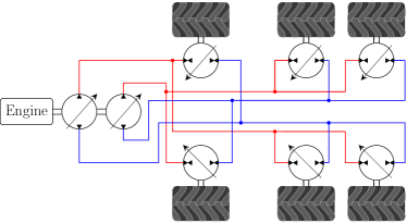
Figure 2: Circuits of the hydrostatic transmission.

2.2 Steering

Steering is actuated by push-pull pairs of hydraulic cylinders, one pair in each of the two articulation joints. Both joints have sensors in the push-pull cylinders to allow measurement of the steering angle. Steering is controlled through the front joint and is regulated using a PI controller with gains $k_{\mathrm{p}}=0.025$, $k_{\mathrm{i}}=0.2~{}\mathrm{s}^{-1}$. An additional PI controller ensures the angle of the rear joint is $56\text{\,}\mathrm{\char 37\relax}$ of the front joint, where the relation is determined by geometry. We tune the rear controller and use a small delay relative to the front to achieve a trade-off between positioning accuracy and the forced pull on the rear parts of the machine. The steering also has a speed threshold which restricts the machine from turning whenever its forward speed is below $0.3\text{\,}\mathrm{k}\mathrm{m}\mathrm{/}\mathrm{h}$.

2.3 Pendulum arm control

The Xt28 has a dedicated ECU for controlling the pendulum arms. The hydraulic pump and valves that are responsible for the suspensions have a hydraulic load-sensing control system. In load-sensing systems, the pump displacement is controlled through a hydraulic feedback line from the actuator valves [16]. Ideally, this ensures a constant flow and makes the system more adaptive to changes in load. The speed of the cylinder is proportional to the flow, and the flow correlates to the valve control signal.

All arm cylinders are equipped with pressure sensors on both the high- and low-pressure sides. The pressure sensors allow for a differential pressure measurement of the cylinder, which is used to estimate the ground force of each wheel.

We can control the pendulum arms in three different modes: using conventional control to achieve automatic active suspensions, passive suspensions, and manual active suspensions. The passive mode runs simultaneously with either automatic active or manual active suspensions. The mode we expose to the DRL controller is the manual active suspensions. We use the conventional controller for active suspensions during experiments to compare it with the DRL controller.

2.3.1 Passive suspensions

The passive mode is based on small pre-pressured hydraulic accumulators, one for each wheel connected to the high-pressure side of each cylinder. The accumulators provide some slack in the system and can absorb the highest impulse forces. Fig. 3 illustrates the hydraulic circuit for a one-wheel suspension.

2.3.2 Automatic active suspensions

The system with automatic suspensions has a customized implementation that runs on the dedicated ECU unit for the pendulum arms. The controller has a cascaded design in three levels: The top level has three P-controllers for roll, pitch, and height along with a fourth controller for ground pressure. The ground pressure controller aims to evenly distribute the normal force among all wheels and requests a force for each arm, considering the uneven weight distribution of the machine. The pitch controller inputs a measurement of the vehicle’s pitch angle and outputs a requested force change between the front and rear arms. Similarly, the roll controller inputs the vehicle’s roll angle and outputs a requested force change between the left and right side arms. The height controller uses the average height of the arms as input and outputs a requested force change of all arms. The outputs of the four subsystems are expressed in terms of requests for each wheel arm, and the resulting setpoint for each arm is simply a weighted sum of all four controller requests. The middle level of the controller is a PID controller that converts the forces into currents corresponding to valve openings. At the lowest level is a hardware controller for electric output currents built into the ECU to ensure the setpoints for the hydraulic valve solenoids.

2.3.3 Manual suspensions

The machine supports “manual suspensions”, which allow direct control of the valves of pendulum cylinders. A single value per arm is used to move the wheel downwards, upwards, or keep still. To provide position control of the wheel suspensions, PI controllers convert the target cylinder positions to valve openings. The cylinder positions, that have a range $[0.0,0.5]~{}\mathrm{m}$, are measured and used as feedback. The PI controllers were tuned on the physical machine to achieve a satisfactory response without overloading the hydraulic system. The resulting gains are $k_{\mathrm{p}}=0.004~{}\mathrm{mm}^{-1}$, $k_{\mathrm{i}}=0.0001~{}\mathrm{mm}^{-1}\mathrm{s}^{-1}$ with a windup limit of 100 as a maximum limit for the error integral.

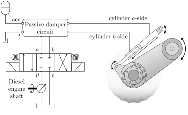
Figure 3: Simplified hydraulic circuit for the suspension of one pendulum arm. The direction control valve above the diesel engine shaft controls the fluid flow to the actuator. Each of the three boxes represents a different valve position, where the centre box indicates the neutral position with both ports closed. The pump and tank are common.

2.4 Pose and velocity measurements

The machine has a global navigation satellite system (GNSS) with dual antennas placed on the cabin’s roof. The system is based on two simpleRTK2B GNSS modules from Ardusimple comprising ZED-F9P5 modules from u-blox. These are connected in a moving base RTK setup with a local base station for correction. The system provides positional data with the capability of cm accuracy. It also provides velocity and heading. To measure the roll and pitch angles, an IMU is placed in the front frame of the vehicle.

2.5 Communication

To read sensors, process data, and control the machine, a hardware interface node is implemented in Robot Operating System (ROS), release Melodic Morenia [17]. The node runs on an onboard Nvidia Jetson and allows easy access to pose and velocity measurements and the vehicle joints using ROS topics. The GNSS is connected to the Jetson with USB and exposed to ROS using the package KumarRobotics ublox. ROS topics regarding joint control and sensing are communicated through the pendulum arms, steering angles, and wheels via the onboard ECUs through CAN-bus interfaces. The ROS network is deployed onboard the machine using a 1 Gbit/s Ethernet connection.

3 Simulation environment

The simulation environment consists of rigid bodies interacting through contacts, friction, and kinematic constraints using the physics engine AGX Dynamics [18].

3.1 Terrains

To represent terrains, we use height maps on a uniform grid with 0.1 m resolution that we interpolate using triangular, piecewise planar elements, to form a continuous surface. The geometric mesh is assigned to a static rigid body that represents the ground. We use Perlin noise [19] to generate terrains with natural variation and embed semi-ellipsoids to represent boulders.

The terrain-wheel contact properties determine how the vehicle interacts with the terrain.

3.2 Vehicle model

The vehicle model is based on a CAD drawing of the original vehicle and has 14 actuated joints. Although it is possible to simulate hydraulic circuits and electronics explicitly, this approach would increase the number of simulation parameters to calibrate and slow down the simulation. Instead, we model the actuator dynamics using 1D constraints.

To achieve steering, we use hinge joints with 1D motors in place of the push-pull pairs at the articulation joints of the real machine. To simulate the hydraulic circuits illustrated in Fig. 2, we model the transmission as two cross-connected differentials connected to a central engine. The engine tries to maintain a target rotational speed of the two input shafts that connect it with the differentials. We represent each differential as a kinematic constraint that distributes torque over three output shafts, ensuring that the average speed matches that of the input shaft. We associate the output shafts with their corresponding wheel axis of rotation. For computational reasons concerning contact detection, we treat the wheels as rigid with spherical shapes.

Linear joints with compliant 1D lock constraints actuate the suspensions. The lock limits the remaining degree of freedom to a fixed position in a soft way to imitate the smoothing and dampening effect of a hydraulic accumulator. This way of modelling the passive suspensions is also intended to compensate for the simplified wheel model. Shifting the rest position of the lock along the axis of the cylinder enables manual position control of the suspensions and effectively extends or contracts the shaft.

To achieve position control similar to the real vehicle, we simulate the PI controllers for suspension and articulation. These controllers offer the same functionality as the real actuators and were tuned to make the model agree with the physical machine in step response experiments. Therefore, the controllers also provide a means for model tuning between the simulated and real machine.

3.3 System identification

To have an accurate model of the actuator dynamics, we design test scenarios that are run on both the real and the simulated platform. The simulation parameters are tuned manually until a given control signal produces a similar enough response from both the real and simulated machine. Special effort is put into calibrating the model’s control of the pendulum arms and the articulated steering.

In total, we tune some 50 parameters during calibration. There are 14 parameters involved in the articulated steering, which affects both the front and rear hinges. These parameters include delays, PID gains, as well as ranges for angles, torques, and angular velocities. The model for pendulum arms has 24 tunable parameters, including PID gains, actuator range, different speed limits for contraction and extension, lock constraint compliance and damping, force range limits, force thresholds, delays, and drift speed. The remaining parameters include the engine torque range, wheel axes rolling resistance, and properties of the wheel-ground contact material, such as Young’s modulus, restitution, friction, and damping coefficients.

3.3.1 Pendulum arms

The pendulum arms’ actuator dynamics is characterised by interactions between the manual and passive suspension systems running in parallel.

Fig. 4 shows an example of a quasi-static calibration test of the pendulum arm control. The test scenario is the following: Starting at standstill with the pendulum arms fully contracted, extend the front and rear hydraulic cylinders while keeping the middle pair contracted. The front and rear cylinders go from minimal to maximal extension and back again in two steps. Note how the real machine struggles to keep the middle pair of arms in place when they are not supported by the ground. Looking at the arm extension curves in this scenario, we see that the real machine is able to use the weight of the chassis to rapidly contract its arms. One can also note that the real machine is faster to extend its rear arms than the front ones. This is explained by the machine being front-heavy when running with an empty bunk and hydraulic coupling effects. To overcome these issues, we considered using different PID gains for each of the three sections as well as different gains for extension and contraction. Ultimately we decided against this to avoid adding more parameters to the model and risk overfitting.

Since distributing the vehicle’s weight on any more than three arms is an underdetermined configuration, it is significantly more difficult to reproduce the load on each arm than to reproduce the cylinder extension. During calibration, we typically settle for agreeing on overall trends such as the ones shown in Fig. 4 and instead try to replicate the sum of the forces on all arms, as seen in Fig. 5. The total vertical force on the arms is consistently larger in simulation than in reality; this is accounted for by simply rescaling the force readings before passing them to the DRL controller.

The pendulum arms in the front section are mounted in the opposite direction of the other four, with the wheel in front of the chassis mount points. As the arms extend, they make a pinching motion toward the ground. Since the hydraulic fluid in the wheel-motors at standstill counteract wheel rotation, this motion can increase the load on the hydraulic cylinders. Since the hydraulic load is used to estimate the tire-ground forces, we will (falsely) register this as an increase in vertical force. This explains the non-constant sum seen in Fig. 5. When the vehicle is at rest, we expect all vertical forces to sum up to the machine’s sprung mass.

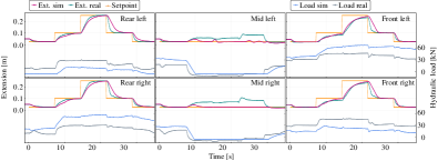
Figure 4: Step responses in arm extension and vertical load per arm in simulation compared to those of the real machine.

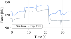
Figure 5: Forces from simulation compared to real-world measurements. Curves show the sum of the estimated vertical force on each wheel during the same calibration test as in Fig. 4.

3.3.2 Steering & Transmission

To model the steering, we implement the relation for the front and rear joints described in Section 2.2 and tune the gains in the simulated PI-controller. Fig. 6 shows results from a test scenario with a sharp S-turn on flat terrain. Note that the simulation does not have any actuator delays in this scenario except for the built-in delay in the rear waist hinge. The large offset in the front angle at around $t=$10\text{\,}\mathrm{s}$$ is a result of regular delay combined with a slightly faster acceleration in simulation, making the machine reach the speed threshold for turning a few moments earlier. The offsets at the start of the final turnaround at $t=$36\text{\,}\mathrm{s}$$ are examples of pure actuator delays.

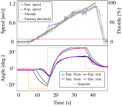
Figure 6: Comparison of articulation hinge angles and forward speed during a steering calibration test. Note that only one signal is used to control both the front and rear hinges.

3.3.3 Model validation

To prevent overfitting, we set aside data from a few of the calibration tests and DRL-controlled test runs and used them as a validation set. Fig. 7 shows the pendulum arm control signals and responses during a live run as the result of a prototype DRL-controller. The vehicle is commanded to drive 25 m straight ahead on flat terrain. Despite the erratic bang-bang control signals, the responses in the simulation show good agreement with the ones from the real experiment.

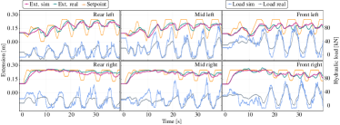
Figure 7: Comparison of arm extension and vertical load per arm sim-vs-real during an agent-controlled test run.

4 Controller

The goal of the DRL controller is to safely and efficiently reach a target pose specified by a planar position and heading. The control system is based on several components, as illustrated in Fig. 8. The reinforcement learning trains the controller, which is supported by PID controllers for the different actuators.

As a safety precaution, to assure that the vehicle cannot overturn, the controller is set to use at most half of the suspension range, i.e. $[0.00,0.25]$ m. For the same reason, we also limit the controller output signal to $30\text{\,}\mathrm{\char 37\relax}$ of full arm movement speed.

4.1 Control policy

The policy is a multivariate Gaussian represented as a neural network with parameters $\theta$ that maps state $s$ to mean action $\mu_{\theta}(s)$. During exploration, the probability of selecting action $a$ in state $s$ is given by $\pi_{\theta}(a|s)=\mathcal{N}(a|\mu_{\theta}(s),\mathrm{diag}(\sigma^{2}))$. The variance vector $\sigma^{2}$ is treated as a standalone parameter, independent of the state.

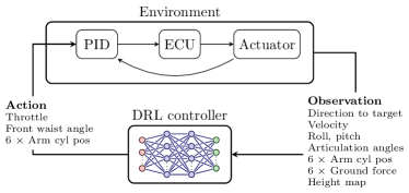
Figure 8: Overview of the control system.

4.2 Observation and action

The controller receives directions $(x,y,\Psi)$ to the target pose and velocity in its local frame of reference as well as the roll and pitch angle. The vehicle configuration is input in terms of the piston displacement for each suspension and both frame articulation angles. To learn about the wheel–terrain interaction, we provide the forces in the hydraulic cylinders. Each force input is scaled by the sum of forces during static equilibrium and clipped to $[-1,1]$. We also include the previous action in the observation space.

The exteroceptive input consists of a local height map that follows the vehicle position and heading in a global frame. The heights are extracted through localization in a global map [6, 20]. A global map can be obtained in advance from aerial laser scans and processed offline to only include the terrain. The local map extends $15\times 10$ m² with a grid of $30\times 20$ points. Heights are taken relative to the reference frame and scaled to be in $[0,1]$.

Given an observation, the controller outputs an 8D action in $[-1,1]$. The action specifies throttle, target angle for the front frame articulation, and target position for each suspension joint.

4.3 Learning control

To train control policies, we use the stable-baselines3 [21] implementation of PPO [22]. The architecture of the policy and value network as well as the hyperparameters are the same as in our previous study [6]. The exception is the discount factor $\gamma=0.995$ to account for longer episodes and the addition of a limit for the Kullback-Leibler divergence of 0.1 between policy updates. We let the simulation run at 60 Hz and use a control frequency of $f_{\mathrm{control}}=10$ Hz.

4.3.1 Reward

The complete reward consists of individual terms, as developed and described in detail in [6], and takes the form

$$r=r_{\mathrm{tar}}+r_{\mathrm{prog}}r_{\mathrm{speed}}r_{\mathrm{head}}r_{\mathrm{forces}}r_{\mathrm{roll}}.$$ (1)

The target reward is defined as $r_{\mathrm{tar}}=k_{\mathrm{tar}}\mathds{1}(\Psi,d_{t})$, where $k_{\mathrm{tar}}$ is a constant set to $5\text{\,}\mathrm{\char 37\relax}$ of the maximum, undiscounted, episodic return and the indicator function $\mathds{1}$ evaluates to 1 at the target and 0 otherwise. Success is defined as being within 0.3 m of the target with less than 9^∘ relative heading and 7.5^∘ roll angle. To densify the signal, we reward progress toward the target as $r_{\mathrm{prog}}=(d_{t-1}-d_{t})f_{\mathrm{control}}$, where $d_{t}$, $d_{t-1}$ is the current and previous distance from the vehicle to the target projected to the horizontal plane. The term $r_{\mathrm{speed}}=\min(1,\exp[k_{\mathrm{speed}}(v_{\mathrm{lim}}-|v|)])$ encourages limited vehicle speeds, where $v_{\mathrm{lim}}=0.8$ m/s, and $k_{\mathrm{speed}}=2$ s/m is a constant manually tuned to control the rate of reward decay for speeds above $v_{\mathrm{lim}}$. Heading alignment is increasingly important as the vehicle approaches the target as $r_{\mathrm{head}}=\exp[-\frac{1}{2}\left(\Psi/(d_{t}/k_{\mathrm{d}})\right)^{2}]$, where the constant $k_{\mathrm{d}}=5$ m is tuned in accord with the turning radius of the vehicle. To limit ground pressure, we consider the standard deviation of normalized ground forces, $\sigma_{\mathrm{forces}}$. We promote even weight distribution through $r_{\mathrm{forces}}=\exp[-\frac{1}{2}\left(\sigma_{\mathrm{forces}}/k_{\mathrm{forces}}\right)^{2}]$, where $k_{\mathrm{forces}}=0.1$. To avoid the risk of overturning, we define the roll reward as $r_{\mathrm{roll}}=\exp[-\frac{1}{2}\left(\phi/k_{\mathrm{\phi}}\right)^{2}]$, where $k_{\mathrm{\phi}}=\pi/16$.

The reward (1) is sufficient to train well-behaved policies but may yield a control signal that exhibits fast switching between or near the control limits. While extremal switching or bang-bang control may be optimal in many continuous control problems [23], it is unsuitable for several reasons. Pure or near bang-bang behaviour may cause wear and tear on the equipment, unnecessary energy consumption, and excite higher-order dynamics that aggravates sim-to-real transfer. Several works address the problem of bang-bang control from DRL controllers by introducing action regularization in the objective function [24] or by constraining the optimization problem [25]. However, with the risk of limiting exploration, we take the common approach of adding a penalty to the reward function.

Striving towards a smooth control signal, we use an additional term in the reward

$$r^{\prime}=r+r_{\Delta_{a}},$$ (2)

where $r_{\Delta_{a}}=\Delta_{a}^{T}M\Delta_{a}$ penalizes the difference between the current and previous action, $\Delta_{a}$. The diagonal matrix $M$ holds a weight factor for each actuator. We use $-0.01$ for the throttle and the steering, and $-0.05$ for the suspensions.

4.3.2 Training

We train control policies on ten environments that run in parallel with different terrains. Before an episode starts, the environment deploys the vehicle with a random heading at a random position within the unit square of the terrain origin. We place the target 25 m away along a circular arc with relative heading $\psi$ sampled uniformly within $\pm\psi_{\mathrm{max}}$. Then, we shift the target heading $\pm\psi_{\mathrm{max}}/2$ relative to $\psi$ so it does not always point in the radial direction.

An episode has a horizon of 45 s, corresponding to 450 control steps. The episode is terminated if the vehicle reaches the target pose or in the event of a terminal condition. A terminal condition occurs if the vehicle exceeds the roll limit of 30^∘, if it misses the target, or if there is contact between anything else than the wheels and the ground.

To modulate difficulty during training, we use a two-lesson curriculum. The first lesson uses uneven but simple terrains without obstacles and heading parameter $\phi_{\mathrm{max}}=\pi/6$. The second lesson focuses on learning to use the suspensions and less emphasis on turning. Therefore it uses $\phi_{\mathrm{max}}=\pi/8$ but has terrains with larger variations and embedded obstacles to represent passable boulders. We change the learning rate from $2.5\times 10^{-4}$ in the first lesson to $1.0\times 10^{-5}$ in the second.

4.4 Narrowing the reality gap

To understand the effect of different strategies to overcome the reality gap, we train policies using three different settings. The nominal setting is to train without any sim-to-real consideration apart from system identification. The second setting uses reward (2), whose additional purpose is to mitigate bang-bang control. The third setting uses the same action penalty and includes observation noise and action delays.

4.4.1 Observation noise

We add independent Gaussian noise to some of the observations at each step. The noise has zero mean with standard deviation taken from sensor data sheets or estimated from calibration experiments, e.g., the measured velocity when standing still or driving with constant speed. We use a standard deviation of 0.005 m for the positional data, 0.075 m/s for planar velocity, 0.025 m/s vertically, and 0.005 rad for the heading. The local height map already contains noise from the original laser scan. From maps collected on a flat parking lot, we estimate a suitable standard deviation that corresponds to 4.5 cm.

4.4.2 Action delays

The intricate hydraulic driveline of the vehicle inherently leads to delays at different time scales for the different actuators. We determine the typical delays by measuring the time from when we send a control signal to when we see any response in the actuator [11]. Our tests reveal that the throttle delay is in the range $[0.2,0.7]$ s, the frame articulation delay in $[0.2,0.5]$ s, and the suspensions delay in $[0.1,0.2]$ s.

Action delays are included during training by sampling a delay for each of the three groups of actuators at the beginning of an episode. Depending on the delay, we withhold actions a number of steps before passing them to the actuators, which then respond immediately.

For the controller to learn about delays, we augment the observation space with a window of previous observations, excluding the height field data. We use a window size of eight considering the control frequency of 10 Hz so that the largest possible delay of 0.7 s can be part of observation history.

4.5 Implementation on the Xt28

The DRL controller is implemented in Python 3.8 and runs on a laptop placed inside the cabin. We employ a Rosbridge [26] for seamless communication between the DRL controller and ROS, regardless of the ROS system, Python version, or packages involved.

To construct the observation space as expected by the policies, we must deal with sensors that run on different frequencies. All sensors run at 100 Hz except the GNSS, which has a frequency of 8 Hz and thus defines the frequency of the DRL controller. While waiting for the GNSS, we store data from the other sensors in running lists. When the GNSS publishes, we average over all sources that have more than one value. The GNSS data is transformed from geodetic to local frame, which is also used to extract the local height map from the elevation model of the environment. Finally, observations are mapped to the ranges used in the simulation before being fed to the policy. The policy outputs a vector of actions that are mapped to their corresponding actuator and published as ROS topics for actuation.

5 Results and discussion

The training and evaluation of the two-step curriculum across three different settings, resulted in four policies of interest: A, B, $\mathrm{C}_{1}$ and $\mathrm{C}_{2}$, see Fig. 9. We suspect that policies $\mathrm{C}_{1}$ and $\mathrm{C}_{2}$ will have the best transfer capabilities to the real vehicle, as they were trained with observation noise, action delays, and reward (2) that includes a penalty for changes in the control signal. Policies A and B are kept for comparison.

Progress during the second lesson is marginal. The reason is either that the terrains with obstacles are too difficult or that the low ground clearance developed during the first lesson is hard to unlearn. Without a higher ground clearance, the chassis frequently collides with obstacles that cause episode termination. We discovered that Policy $\mathrm{C}_{2}$ was better than $\mathrm{C}_{1}$ at overcoming obstacles but degraded in terms of a smooth control signal, leading us to proceed by evaluating both of them on the physical machine.

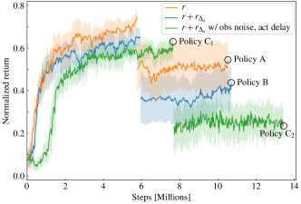
Figure 9: Learning curves plotted over a two-lesson curriculum, evaluated for 20 episodes, once every $25\text{\,}\mathrm{k}$ steps. We chose the best policy from the first lesson in terms of normalized return as starting point for the second. Among the policies developed in the second lesson, the final selections are policies A, B, and $\mathrm{C}_{2}$. Policy $\mathrm{C}_{2}$ was chosen for its high success rate of $95\text{\,}\mathrm{\char 37\relax}$. Additionally, we retain Policy $\mathrm{C}_{1}$.

The field experiments took place at Troëdsson Teleoperation Lab, run by Skogforsk and located in Jälla, Sweden. The area consists of a large gravel parking surrounded by blocky forest terrain. Two years before the field experiment, the entire area was scanned using airborne photogrammetry that resulted in a digital surface model with a resolution of $0.25\text{\,}\mathrm{m}$. Combining the geotagged surface model with the onboard RTK GNSS allows us to extract local height maps that are part of the controller observation space.

We emphasize that the main focus of the remaining experiments is to evaluate the sim-to-real transfer. The crucial aspect is that the strategies learnt in simulation also work well in reality, so for the analysis to have meaning, it matters if these strategies present what we desire and aim for when shaping the reward functions. In that sense, performance is also relevant.

5.1 Basic driving

We evaluate policy performance in terms of reward (1) for three scenarios on flat ground: driving straight, turning left, and right, see Fig. 10. The simulation cases vary in complexity from perfect observations and immediate action to noisy observations and delayed actions. The real data was collected on the flat parking space.

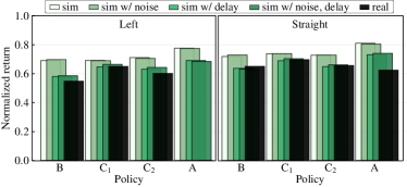
Figure 10: Policy performance in simulation compared to reality according to the base reward. The target is placed on flat ground 25 m away straight ahead or to the left, corresponding to an initial relative heading of $23^{\circ}$. The right case was omitted due to symmetry. Unfortunately, an error in the GNSS caused unusable data for Policy A for left and right turns.

Among the four policies, $\mathrm{C}_{1}$ shows the best transfer capabilities over all scenarios, while policies B and  $\mathrm{C}_{2}$ are comparable. On flat terrain, Policy $\mathrm{C}_{1}$ is expected to outperform Policy $\mathrm{C}_{2}$ because the latter proceeds to train on rougher terrain with boulders. This causes it to trade specializing in flat terrain to handle avoidance of obstacles and practice a more active use of the suspensions. Despite no such experience from training, the base Policy A performs the best in simulation even with observation noise and action delays but sees a large drop when deployed in reality. Overall, we note that adding delays to simulations has the most pronounced effect on policies that lack experience with delays, while the impact of noise is minor for all policies.

Evaluating performance in terms of the reward does not justify the true experience of witnessing the field tests. For some runs, the real machine displayed shakiness, pulsating sound from the hydraulic motors, and other unwanted behaviour that we had not anticipated and therefore not included in any reward function.

In the simulations, all four policies accomplish smooth motions, a necessary characteristic for real-world applications. To study the real motions, we plot the trajectories relative to the initial pose, see the left panel in Fig. 11. Policies A and B yield wiggly trajectories compared to $\mathrm{C}_{1}$ and $\mathrm{C}_{2}$ that progress towards the target smoothly. The target is reached in all three cases for $\mathrm{C_{2}}$, two out of three times for $\mathrm{C_{1}}$, and only once for Policy B. The right panel in Fig. 11 shows the control action for the throttle and steering angle with the target straight ahead. As is clear, Policy A exhibits bang-bang control, which in our case works well in simulation but transfers poorly to reality. During the experiments, we could hear the hydraulic motors struggling rhythmically to build up and release pressure. The signal from Policy $\mathrm{C}_{1}$ resulted in smooth motions and overall best behaviour from a visual and auditorial standpoint among all four policies. The results confirm the importance of including actuator delays during training. The results also show that, without some kind of regularization for actions, the policy is likely to converge to an unwanted bang-bang controller.

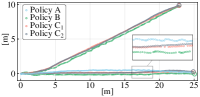
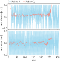
Figure 11: Left: Physical trajectories on even terrain, where a large circle at the endpoint indicates reaching the target. The target pose is placed 25 m away with initial relative headings $0^{\circ}$ and $23^{\circ}$, respectively. Policy A only has one trajectory due to an error in the GNSS for the other two. Right: Policy action for throttle and front steering angle in the case of driving straight.

To mimic a practical use case, we test Policy $\mathrm{C}_{1}$ on a sequence of targets that trace out a predefined route. Given the initial vehicle pose, we use a simple GUI application to manually choose subsequent target poses on a 2D map of the digital elevation model. To see how the controller handles situations incompatible with the kinematic constraints of the vehicle and unseen states, some subsequent targets require impossibly sharp turns. The experiments are carried out in reality as well as in simulation, see Fig. 12. In general, the controller succeeds to follow the route and trace out a smooth trajectory in both reality and simulation. The decision-making of the policy is not straightforward to explain. For some reason, the real case starts to deviate from the simulation at the first left turn in Fig. 12, causing the controller to end up in a challenging situation. From that moment on, the following targets become increasingly difficult, to the point where the targets in the upper left part are missed almost immediately. As a consequence, the controller then focuses on the next target, which exacerbates the offset compared to the simulation case. Eventually, the controller recovers to complete the route and does so without presenting any high-risk manoeuvres. Apart from the aforementioned deviations, the real and simulated motions overlap, showing adequate transfer capabilities in terms of driving and steering.

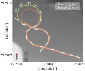
Figure 12: Real and simulated trajectories starting in the bottom right executed by Policy $\mathrm{C}_{1}$ when set to follow a sequence of target poses. Target positions are drawn as white circles, and the corresponding arrows show the target heading. The vehicle is true to scale.

5.2 Vibration course

To study the use of the height map information for controlling the arms, we use a vibration course. It consists of obstacles that are normally bolted to a concrete fundament following a standardized design and layout with the purpose to compare the performance of different forwarders, see Fig. 13. We use approximately the same layout and attach the obstacles to the gravel ground.

During the field experiments, we compare two cases of driving through the vibration course, with and without adding obstacles to the digital surface model. In the latter case, the controller only sees the ground and must rely fully on the proprioceptive information to physically feel the obstacles. There was no clear difference between the two runs, but with several obstacles, noisy measurements, and variations in initial conditions, the results were difficult to analyze.

Instead, we resort to simulation with the motivation that if the controller does not make use of the height map there, then it will not do so in reality either. In simulation, we embed the obstacles in the surface model and perform two experiments identical to the field experiments, except we use a completely flat ground to avoid noisy measurements, see Fig. 14. As can be seen, the information from the height map has no clear effect on the arm control, so we conclude that the controller mainly uses proprioceptive information for decision-making. We did note that, for other constant height maps of extreme values, the controller gets stuck or performs poorly, indicating that the local heights are of some use. The use is, however, not for look-ahead planning, as we had hoped and anticipated from previous work [6].

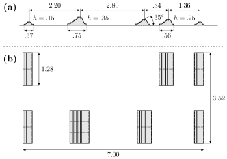
Figure 13: Illustration of the vibration course from a side view (a) and top-down view (b). The machine drives from left to right in the figure. All values are in metres.

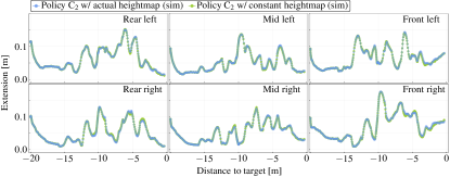
Figure 14: Comparison between two simulation runs over the vibration course, one with obstacles included in the height map and one without.

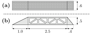
Figure 15: Schematic of the ramp obstacle from a top-down view (a) and side view (b). The vehicle drives from left to right in the figure. All values are in metres.

5.3 Obstacles

To study the use of the suspensions in isolation, we use a ramp wide enough to fit one wheel, see Fig. 15. For this case, the controller uses Policy $\mathrm{C}_{2}$, which has trained on terrains with boulders, including observation noise and action delays. The primary objective of this experiment is to evaluate the sim-to-real transfer capability, with a secondary focus on examining the learnt control strategy.

The DRL controller successfully manages to control the arms to overcome the big ramp and reach the target placed 15 m straight ahead. To make a comparison with the simulation, we use the 3D representation of the scanned gravel parking area with embedded obstacles, see Fig. 16. The vehicle and target are placed at the same coordinates as during the real experiment. A sim-vs-real video is available as supplementary material, found here: http://umit:cs:umu:se/s2r-ascdrl/ When we study the arm extensions, it is clear that the strategy developed in simulation to control the suspensions work equally well in reality, see Fig. 17. As the front left wheel moves up the ramp, the controller tries to lift it while pressing down on the other side to maintain levelling and balance ground forces. We see similar behaviour for the wheels on the middle and rear sections. With locked suspensions, the vehicle would have a maximum roll angle of roughly 14 degrees, which with the DRL control is reduced to 6 degrees.

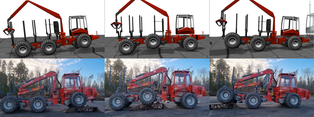
Figure 16: Sim-vs-real comparison of Policy $\mathrm{C}_{2}$ driving over the large ramp. Images are mirrored to run from left to right.

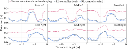
Figure 17: Arm extension for all wheels when driving over the large ramp. The real and simulation case uses Policy $\mathrm{C}_{2}$. In the human case, the suspensions were regulated by a conventional controller that has a nominal extension of 0.25 m and twice the range of the DRL controllers.

As seen in Fig. 17, we also compare the DRL controller to the automatic suspension control with a human operator for steering and throttle. The trends in arm extensions show a clear resemblance, indicating that the DRL controller has learnt a similar strategy to balance ground forces. The human case results in a maximum roll angle of 4 degrees, although the comparison is not entirely fair. For reasons of safety and comfort, the human operator drove significantly slower than the DRL controller, giving more time for the actuators to level out, and was allowed to use twice the suspension range. When placing the ramp on the other side of the vehicle, the DRL controller got stuck on the chassis. However, considering the small margins with the limited suspension range, this is a challenging scenario.

Having previously established that the local height map is not significant in controlling suspensions, the hydraulic load must act as the primary feedback. However, since the system identification in Section 3.3.1 uses calibration scenarios on level ground it is not clear how well it applies to the ramp experiments. Fig. 18 compares the normalized hydraulic loads when passing the ramp, which show qualitative agreement, indicating that the system identification has captured the dynamics beyond the calibration scenarios. The main difference between the curves is that the simulation shows larger fluctuations. This is because the simulation model assumes rigid wheels and compliant lock constraints for the suspensions, whereas the real system has flexible tires and hydraulic accumulators that provide additional smoothing and damping. While these differences do not seem to affect performance, they imply the need for a tire model to increase simulation fidelity. Interestingly, the “noise” in simulated hydraulic load has the same effect as domain randomization. This explains why the policies are so robust to the domain shift and perform better than expected in the real world, despite not adding noise to the observations for the hydraulic load.

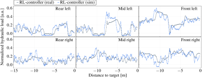
Figure 18: Hydraulic load on the suspensions when driving over the large ramp, where both the real and the simulation case use Policy $\mathrm{C}_{2}$.

6 Conclusion

We conclude that an accurate model of the actuator dynamics, modelling action delays, and preventing the emergence of bang-bang control are necessary to handle the sim-to-real gap for heavy vehicles with hydraulic actuators in rough terrain.

Actuator models using 1D motor constraints and system identification produce sufficiently accurate models of the hydraulic actuators. This approach is faster to simulate and requires fewer parameters for tuning than modelling the actual hydraulic circuits. Moreover, some of the success is attributed to the low-level PID controllers, which operate independently of the DRL controller and are responsible for the final actuation of the system. Tuning the PIDs in simulations allows slack in modelling errors and can mitigate the effect of unmodelled actuator dynamics. A higher fidelity simulation would involve a tire model but does not appear to be necessary for the studied control task. Natural terrain may amplify the effects of the simplified tire model. However, due to wet November conditions, we were unable to transport the vehicle to the areas of blocky natural terrain.

Aside from the actuator model, including actuator delays during training have the most prominent effect on sim-to-real transfer. The impact of adding observation noise is unclear since the simulated ground forces, the primary feedback for suspension control, are already noisy. As a result, the effect on controller robustness is similar to domain randomization.

The controllers we present have room for improvement when it comes to obstacles and making use of perceptual information. Due to slow learning, the current study did not reach the level of learning to distinguish between passable and unpassable obstacles as in our previous work [6]. This is partly attributed to the vehicle model of the hydrostatic transmission with two exotic differential gears. Compared to the previous study, which employed individual wheel torque control, the current transmission presents a more complex state-action-reward mapping, necessitating further effort. Another potential reason is the limited available suspension range and speed enforced for safety reasons, which restricts exploration. To address these complexities, a promising approach is to take inspiration from similar work in legged locomotion, e.g., by using an attention-based recurrent encoder [9]. These encoders could simplify learning about the transmission and enhance the use of the suspensions by coupling proprioceptive and exteroceptive information in look-ahead planning. On the upside, we now know that the control strategies learnt in simulation transfer to reality.

7 Acknowledgements

The research was supported in part by Troëdsson Teleoperation Lab, Mistra Digital Forest, Algoryx Simulation AB, Swedish National Infrastructure for Computing at High-Performance Computing Center North (HPC2N), eSSENCE, and eXtractor AB.

8 Declaration of generative AI and AI-assisted technologies in the writing process

During the preparation of this work, the authors used ChatGPT 3.5 to enhance text clarity, fluency, and conciseness. After using this tool, the authors reviewed and edited the content as needed and take full responsibility for the content of the publication.

References

- [1] H. Hu, K. Zhang, A. H. Tan, M. Ruan, C. Agia, G. Nejat, A sim-to-real pipeline for deep reinforcement learning for autonomous robot navigation in cluttered rough terrain, IEEE Robotics and Automation Letters 6 (4) (2021) 6569–6576.
- [2] P. Egli, M. Hutter, A general approach for the automation of hydraulic excavator arms using reinforcement learning, IEEE Robotics and Automation Letters 7 (2) (2022) 5679–5686.
- [3] W. Zhao, J. P. Queralta, T. Westerlund, Sim-to-real transfer in deep reinforcement learning for robotics: a survey, in: 2020 IEEE symposium series on computational intelligence (SSCI), IEEE, 2020, pp. 737–744.
- [4] G. Dulac-Arnold, N. Levine, D. J. Mankowitz, J. Li, C. Paduraru, S. Gowal, T. Hester, Challenges of real-world reinforcement learning: definitions, benchmarks and analysis, Machine Learning 110 (9) (2021) 2419–2468.
- [5] O. Gelin, R. Björheden, Concept evaluations of three novel forwarders for gentler forest operations, Journal of Terramechanics 90 (2020) 49–57.
- [6] V. Wiberg, E. Wallin, T. Nordfjell, M. Servin, Control of rough terrain vehicles using deep reinforcement learning, IEEE Robotics and Automation Letters 7 (1) (2021) 390–397.
- [7] R. Kirk, A. Zhang, E. Grefenstette, T. Rocktäschel, A survey of generalisation in deep reinforcement learning, arXiv preprint arXiv:2111.09794 (2021).
- [8] X. B. Peng, M. Andrychowicz, W. Zaremba, P. Abbeel, Sim-to-real transfer of robotic control with dynamics randomization, in: 2018 IEEE international conference on robotics and automation (ICRA), IEEE, 2018, pp. 3803–3810.
- [9] T. Miki, J. Lee, J. Hwangbo, L. Wellhausen, V. Koltun, M. Hutter, Learning robust perceptive locomotion for quadrupedal robots in the wild, Science Robotics 7 (62) (2022) eabk2822.
- [10] S. Choi, G. Ji, J. Park, H. Kim, J. Mun, J. H. Lee, J. Hwangbo, Learning quadrupedal locomotion on deformable terrain, Science Robotics 8 (74) (2023) eade2256.
- [11] J. Tan, T. Zhang, E. Coumans, A. Iscen, Y. Bai, D. Hafner, S. Bohez, V. Vanhoucke, Sim-to-real: Learning agile locomotion for quadruped robots, arXiv preprint arXiv:1804.10332 (2018).
- [12] J. Ibarz, J. Tan, C. Finn, M. Kalakrishnan, P. Pastor, S. Levine, How to train your robot with deep reinforcement learning: lessons we have learned, The International Journal of Robotics Research 40 (4-5) (2021) 698–721.
- [13] T. Haarnoja, A. Zhou, K. Hartikainen, G. Tucker, S. Ha, J. Tan, V. Kumar, H. Zhu, A. Gupta, P. Abbeel, et al., Soft actor-critic algorithms and applications, arXiv preprint arXiv:1812.05905 (2018).
- [14] T. Xiao, E. Jang, D. Kalashnikov, S. Levine, J. Ibarz, K. Hausman, A. Herzog, Thinking while moving: Deep reinforcement learning with concurrent control, arXiv preprint arXiv:2004.06089 (2020).
-
[15]
A. Dell’ Amico, L. Ericson, F. Henriksen, P. Krus,
Modelling and
experimental verification of a secondary controlled six-wheel pendulum arm
forwarder (2015).
URL http://urn.kb.se/resolve?urn=urn:nbn:se:liu:diva-122390 - [16] Z. Yan, L. Ge, L. Quan, Energy-efficient electro-hydraulic power source driven by variable-speed motor, Energies 15 (13) (2022). doi:10.3390/en15134804.
- [17] M. Quigley, K. Conley, B. Gerkey, J. Faust, T. Foote, J. Leibs, R. Wheeler, A. Y. Ng, et al., Ros: an open-source robot operating system, in: ICRA workshop on open source software, Vol. 3, Kobe, Japan, 2009, p. 5.
-
[18]
Algoryx Simulations,
AGX
Dynamics (Feb. 2022).
URL https://www.algoryx.se/documentation/complete/agx/tags/latest/doc/UserManual/source/index.html - [19] K. Perlin, An image synthesizer, ACM Siggraph Computer Graphics 19 (3) (1985) 287–296.
- [20] Q. Li, P. Nevalainen, J. Peña Queralta, J. Heikkonen, T. Westerlund, Localization in unstructured environments: Towards autonomous robots in forests with delaunay triangulation, Remote Sensing 12 (11) (2020) 1870.
-
[21]
A. Raffin, A. Hill, A. Gleave, A. Kanervisto, M. Ernestus, N. Dormann,
Stable-baselines3: Reliable
reinforcement learning implementations, Journal of Machine Learning Research
22 (268) (2021) 1–8.
URL http://jmlr.org/papers/v22/20-1364.html - [22] J. Schulman, F. Wolski, P. Dhariwal, A. Radford, O. Klimov, Proximal policy optimization algorithms, arXiv preprint arXiv:1707.06347 (2017).
- [23] T. Seyde, I. Gilitschenski, W. Schwarting, B. Stellato, M. Riedmiller, M. Wulfmeier, D. Rus, Is bang-bang control all you need? solving continuous control with bernoulli policies, Advances in Neural Information Processing Systems 34 (2021) 27209–27221.
- [24] S. Mysore, B. Mabsout, R. Mancuso, K. Saenko, Regularizing action policies for smooth control with reinforcement learning, in: 2021 IEEE International Conference on Robotics and Automation (ICRA), IEEE, 2021, pp. 1810–1816.
- [25] S. Bohez, A. Abdolmaleki, M. Neunert, J. Buchli, N. Heess, R. Hadsell, Value constrained model-free continuous control, arXiv preprint arXiv:1902.04623 (2019).
- [26] C. Crick, G. Jay, S. Osentoski, B. Pitzer, O. C. Jenkins, Rosbridge: Ros for non-ros users, in: Robotics Research: The 15th International Symposium ISRR, Springer, 2017, pp. 493–504.