Adversarial Training Should Be Cast as a
Non-Zero-Sum Game

Abstract

One prominent approach toward resolving the adversarial vulnerability of deep neural networks is the two-player zero-sum paradigm of adversarial training, in which predictors are trained against adversarially-chosen perturbations of data. Despite the promise of this approach, algorithms based on this paradigm have not engendered sufficient levels of robustness, and suffer from pathological behavior like robust overfitting. To understand this shortcoming, we first show that the commonly used surrogate-based relaxation used in adversarial training algorithms voids all guarantees on the robustness of trained classifiers. The identification of this pitfall informs a novel non-zero-sum bilevel formulation of adversarial training, wherein each player optimizes a different objective function. Our formulation naturally yields a simple algorithmic framework that matches and in some cases outperforms state-of-the-art attacks, attains comparable levels of robustness to standard adversarial training algorithms, and does not suffer from robust overfitting.

1 Introduction

A longstanding disappointment in the machine learning (ML) community is that deep neural networks (DNNs) remain vulnerable to seemingly innocuous changes to their input data including nuisances in visual data [1, 2, 3, 4, 5], sub-populations [6, 7, 8, 9], and distribution shifts [10, 11, 12, 13, 14]. Prominent amongst these vulnerabilities is the setting of adversarial examples, wherein it has been conclusively shown that imperceptible, adversarially-chosen perturbations can fool state-of-the-art classifiers parameterized by DNNs [15, 16, 17, 18, 19]. In response, a plethora of research has proposed so-called adversarial training (AT) algorithms [20, 21, 22, 23, 24, 25, 26], which are designed to improve robustness against adversarial examples.

AT is ubiquitously formulated as a two-player zero-sum game, where both players—often referred to as the defender and the adversary—respectively seek to minimize and maximize the classification error. However, this zero-sum game is not implementable in practice as the discontinuous nature of the classification error is not compatible with first-order optimization algorithms. To bridge this gap between theory and practice, it is commonplace to replace the classification error with a smooth surrogate loss (e.g., the cross-entropy loss) which is amenable to gradient-based optimization [25, 27]. And while this seemingly harmless modification has a decades-long tradition in the ML literature due to the guarantees it imparts on non-adversarial objectives [28, 29, 30], there is a pronounced gap in the literature regarding the implications of this relaxation on the standard formulation of AT.

As the field of robust ML has matured, surrogate-based AT algorithms (see, e.g., [25, 27, 26, 31]) have collectively ushered in significant progress toward designing stronger attacks and obtaining more robust defenses [32]. However, despite these advances, recent years have witnessed a plateau in robustness measures on leaderboards such as RobustBench, resulting in the widely held beliefs that robustness and accuracy may be irreconcilable [33, 34, 35] and that robust generalization requires significantly more data [36, 37, 38]. Moreover, various phenomena such as robust overfitting [39] and insufficient robustness evaluation [40] have indicated that progress has been overestimated [41]. To combat these pitfalls, state-of-the-art algorithms increasingly rely on ad-hoc regularization schemes [42, 27, 43, 44, 45], weight perturbations [46, 47, 48], and heuristics such as multiple restarts [25], carefully crafted learning rate schedules [39], and convoluted stopping conditions [41], all of which contribute to an unclear set of best practices and a growing literature concerned with identifying flaws in various AT schemes [49].

Motivated by these challenges, we argue that the pervasive surrogate-based zero-sum approach to AT suffers from a fundamental flaw. Our analysis of the standard minimax formulation of AT reveals that maximizing a surrogate like the cross-entropy provides no guarantee that the the classification error will increase, resulting in weak adversaries and ineffective AT algorithms. In identifying this shortcoming, we prove that to preserve guarantees on the optimality of the classification error objective, the defender and the adversary must optimize different objectives, resulting in a non-zero-sum game. This leads to a novel, yet natural bilevel formulation [50] of AT in which the defender minimizes an upper bound on the classification error, while the attacker maximizes a continuous reformulation of the classification error. We then propose an algorithm based on our formulation which is free from heuristics and ad hoc optimization techniques. Our empirical evaluations reveal that our approach matches the test robustness achieved by the state-of-the-art, yet highly heuristic approaches such as AutoAttack, and that it eliminates the problem of robust overfitting.

Contributions. We summarize our contributions in the following bullets.

• New formulation for adversarial robustness. Starting from the discontinuous minmax formulation of AT with respect to the 0-1 loss, we derive a novel continuous bilevel optimization formulation, the solution of which guarantees improved robustness against the optimal adversary.

• New adversarial training algorithm. We derive a new, heuristic-free algorithm (Algorithm 2) based on our bilevel formulation, and show that offers strong robustness on CIFAR-10.

• Elimination of robust overfitting. Without the need of heuristic modifications, our algorithm does not suffer from robust overfitting (RO). This suggest that RO is an artifact of the use of improper surrogates in the original AT paradigm, and that the use of a correct optimization formulation is enough to solve it.

• State-of-the-art robustness evaluation. We show that our proposed optimization objective for the adversary yields a simple algorithm that matches the performance of the state-of-the-art, yet highly complex AutoAttack method, on classifiers trained on CIFAR-10.

2 The promises and pitfalls of adversarial training

2.1 Preliminaries: Training DNNs with surrogate losses

We consider a $k$-way classification setting, wherein data arrives in the form of instance-label pairs $(X,Y)$ drawn i.i.d. from an unknown joint distribution $\mathcal{D}$ taking support over $\mathcal{X}\times\mathcal{Y}\subseteq\mathbb{R}^{d}\times[K]$, where $[K]:=\{1,\dots,K\}$. Given a suitable hypothesis class $\mathcal{F}$, one fundamental goal in this setting is to select an element $f\in\mathcal{F}$ which correctly predicts the label $Y$ of a corresponding instance $X$. In practice, this hypothesis class $\mathcal{F}$ often comprises functions $f_{\theta}:\mathbb{R}^{d}\to\mathbb{R}^{K}$ which are parameterized by a vector $\theta\in\Theta\subset\mathbb{R}^{p}$, as is the case when training DNNs. In this scenario, the problem of learning a classifier that correctly predicts $Y$ from $X$ can written as follows:

$$\min_{\theta\in\Theta}\mathbb{E}\bigg{\{}\operatorname*{arg\,max}_{i\in[K]}f_{\theta}(X)_{i}\neq Y\bigg{\}}$$ (1)

Here $f_{\theta}(X)_{i}$ denotes the $i^{\text{th}}$ component of the logits vector $f_{\theta}(X)\in\mathbb{R}^{K}$ and we use the notation $\{A\}$ to denote the indicator function of an event $A$, i.e., $\{A\}:=\mathbb{I}_{A}(\cdot)$. In this sense, $\{\operatorname*{arg\,max}_{i\in[K]}f_{\theta}(X)_{i}\neq Y\}$ denotes the classification error of $f_{\theta}$ on the pair $(X,Y)$.

Prominent among the barriers to solving (1) in practice is the fact that the classification error is a discontinuous function of $\theta$, which in turn renders continuous first-order methods (e.g., gradient descent) intractable. Fortunately, this pitfall can be resolved by minimizing a surrogate loss function $\ell:[k]\times[k]\to\mathbb{R}$ in place of the classification error [29, §12.3]. For minimization problems, surrogate losses are chosen to be differentiable upper bounds of the classification error of $f_{\theta}$, in the sense that

$$\bigg{\{}\operatorname*{arg\,max}_{i\in[K]}f_{\theta}(X)_{i}\neq Y\bigg{\}}\leq\ell(f_{\theta}(X),Y).$$ (2)

This inequality gives rise to a differentiable counterpart of (1) which is amenable to minimization via first-order methods and can be compactly expressed in the following optimization problem:

$$\min_{\theta\in\Theta}\mathbb{E}\>\ell(f_{\theta}(X),Y).$$ (3)

Examples of commonly used surrogates are the hinge loss and the cross-entropy loss. Crucially, the inequality in (2) guarantees that the problem in (3) provides a solution that decreases the classification error [28], which, as discussed above, is the primary goal in supervised classification.

2.2 The pervasive setting of adversarial examples

For common hypothesis classes, it is well-known that classifiers obtained by solving (3) are sensitive to seemingly benign changes to their input data. Among these vulnerabilities, perhaps the most well-studied is the setting of adversarial examples, wherein a plethora of research has demonstrated that state-of-the-art classifiers can be fooled by small, adversarially-chosen perturbations [15, 16, 17, 18, 19]. In other words, given an instance label pair $(X,Y)$, it is relatively straightforward to find perturbations $\eta\in\mathbb{R}^{d}$ with small norm $\left|\left|\eta\right|\right|\leq\epsilon$ for some fixed $\epsilon>0$ such that

$$\operatorname*{arg\,max}_{i\in[K]}f_{\theta}(X)_{i}=Y\qquad\text{and}\qquad\operatorname*{arg\,max}_{i\in[K]}f_{\theta}(X+\eta)_{i}\neq\operatorname*{arg\,max}_{i\in[K]}f_{\theta}(X)_{i}.$$ (4)

The task of finding such perturbations $\eta$ which cause the classifier $f_{\theta}$ to misclassify perturbed data points $X+\eta$ can be compactly cast as the following maximization problem:

$$\eta^{\star}\in\operatorname*{arg\,max}_{\eta:\|\eta\|\leq\epsilon}\bigg{\{}\operatorname*{arg\,max}_{i\in[K]}f_{\theta}(X+\eta)_{i}\neq Y\bigg{\}}$$ (5)

Here, if both of the expressions in (4) hold for the perturbation $\eta=\eta^{\star}$, then the perturbed instance $X+\eta^{\star}$ is called an adversarial example for $f_{\theta}$ with respect to the instance-label pair $(X,Y)$.

Due to prevalence of adversarial examples, there has been pronounced interest in solving the robust analog of (1), which is designed to find classifiers that are insensitive to small perturbations. This robust analog is ubiquitously written as the following a two-player zero-sum game with respect to the discontinuous classification error:

$$\min_{\theta\in\Theta}\mathbb{E}\bigg{[}\max_{\eta:\|\eta\|\leq\epsilon}\bigg{\{}\operatorname*{arg\,max}_{i\in[K]}f_{\theta}(X+\eta)_{i}\neq Y\bigg{\}}\bigg{]}$$ (6)

An optimal solution $\theta^{\star}$ for (6) yields a model $f_{\theta^{\star}}$ that achieves the lowest possible classification error despite the presence of adversarial perturbations. For this reason, this problem—wherein the interplay between the maximization over $\eta$ and the minimization over $\theta$ comprises a two-player zero-sum game— is the starting point for numerous algorithms which aim to improve robustness.

2.3 Surrogate-based approaches to robustness

As discussed in § 2.1, the discontinuity of the classification error complicates the task of finding adversarial examples, as in (5), and of training against these perturbed instances, as in (6). One appealing approach toward overcoming this pitfall is to simply deploy a surrogate loss in place of the classification error inside (6), which gives rise to the following pair of optimization problems:

$$\eta^{\star}\in\operatorname*{arg\,max}_{\eta:\left|\left|\eta\right|\right|\leq\epsilon}\ell(f_{\theta}(X+\eta),Y)$$ (7)

$$\min_{\theta\in\Theta}\mathbb{E}\left[\max_{\eta:\|\eta\|\leq\epsilon}\ell(f_{\theta}(X+\eta),Y)\right]$$ (8)

Indeed, this surrogate-based approach is pervasive in practice. Madry et al.’s seminal paper on the subject of adversarial training employs this formulation [25], which has subsequently been used as the starting point for numerous AT schemes [20, 21, 22, 25, 26].

Pitfalls of surrogate-based optimization. Despite the intuitive appeal of this paradigm, surrogate-based adversarial attacks are known to overestimate robustness [51, 52, 41], and standard adversarial training algorithms are known to fail against strong attacks. Furthermore, this formulation suffers from pitfalls such as robust overfitting [39] and trade-offs between robustness and accuracy [53, 54]. To combat these shortcomings, empirical adversarial attacks and defenses have increasingly relied on heuristics such as multiple restarts, variable learning rate schedules [41], and carefully crafted initializations, resulting in a widening gap between the theory and practice of adversarial learning. In the next section, we argue that these pitfalls can be attributed to the fundamental limitations of (8).

3 Non-zero-sum formulation of adversarial training

3.1 Fundamental limitations of surrogates in adversarial learning

From an optimization perspective, the surrogate-based approaches to adversarial evaluation and training outlined in § 2.3 engenders two fundamental limitations.

• Limitation I: Weak attackers. In the adversarial evaluation problem of (7), the adversary maximizes an upper bound on the classification error. This means that any solution $\eta^{\star}$ to (7) is not guaranteed to increase the classification error in (5), resulting in weakened adversaries which are misaligned with the goal of finding adversarial examples that fool DNNs. Indeed, when the surrogate is an upper bound on the classification error, the only conclusion about the adversarial perturbation $\eta^{\star}$ obtained from (7) and its true objective (5) is:

  $$\bigg{\{}\operatorname*{arg\,max}_{i\in[K]}f_{\theta}(X+\eta^{\star})_{i}\neq Y\bigg{\}}\leq\max_{\eta:\left|\left|\eta\right|\right|\leq\epsilon}\ell(f_{\theta}(X+\eta),Y)$$ (9)

  Notably, the right hand side of (9) can be arbitrarily large while the left hand side can simultaneously be equal to zero, i.e., the problem in (7) can fail to produce an adversarial example, even at optimality. Thus, while it is known empirically that attacks based on (7) tend to overestimate robustness [41, 52, 55], we show that this shortcoming is evident a priori.

• Limitation II: Ineffective defenders. Because attacks which seek to maximize upper bounds on the classification error are not proper surrogates for the classification error (c.f., Limitation I), training a model $f_{\theta}$ on such perturbations does not guarantee any improvement in robustness. Therefore, AT algorithms which seek to solve (8) are ineffective in that they do not optimize the worst-case classification error. For this reason, it should not be surprising that robust overfitting [39] occurs for models trained to solve eq. 8.

Both of these limitations arise directly by virtue of rewriting (7) and (8) with the surrogate loss $\ell$. Therefore, to summarize, there is a distinct tension between the efficient, yet misaligned paradigm of surrogate-based adversarial training with the principled, yet intractable paradigm of minimax optimization on the classification error. In the remainder of this section, we resolve this tension by decoupling the optimization problems of the adversary and the training algorithm.

3.2 Decoupling adversarial attacks and defenses

Our starting point is the two-player zero-sum formulation in (6). Observe that this minimax optimization problem can be equivalently cast as a bilevel optimization problem:

$$\min_{\theta\in\Theta} \mathbb{E}\bigg{\{}\operatorname*{arg\,max}_{i\in[K]}f_{\theta}(X+\eta^{\star})_{i}\neq Y\bigg{\}}$$ (10)

$$\operatorname*{subject\,\,to\quad} \eta^{\star}\in\operatorname*{arg\,max}_{\eta:\>\|\eta\|\leq\epsilon}\bigg{\{}\operatorname*{arg\,max}_{i\in[K]}f_{\theta}(X+\eta)_{i}\neq Y\bigg{\}}$$ (11)

While this problem still constitutes a zero-sum game, the role of the attacker (the constraint in (11)) and the role of the defender (the objective in (10)) are now decoupled. From this perspective, the tension engendered by introducing surrogate losses is laid bare: the attacker ought to maximize a lower bound of the classification error (c.f., Limitation I), whereas the defender ought to minimize an upper bound on the classification error (c.f., Limitation II). This implies that to preserve guarantees on optimality, the attacker and defender must optimize separate objectives. In what follows, we discuss these objectives for the attacker and defender in detail.

The attacker’s objective. We first address the role of the attacker. To do so, we define the negative margin $M_{\theta}(X,Y)$ of the classifier $f_{\theta}$ as follows:

$$M_{\theta}:\mathcal{X}\times\mathcal{Y}\to\mathbb{R}^{k},\qquad M_{\theta}(X,Y)_{j}\triangleq f_{\theta}(X)_{j}-f_{\theta}(X)_{Y}$$ (12)

We call $M_{\theta}(X,Y)$ the negative margin because a positive value of (12) corresponds to a misclassification. As we show in the following proposition, the negative margin function (which is differentiable) provides an alternative characterization of the classification error.

Proposition 1.

Given a fixed data pair $(X,Y)$, let $\eta^{\star}$ denote any maximizer of $M_{\theta}(X+\eta,Y)_{j}$ over the classes $j\in[K]-\{Y\}$ and perturbations $\eta\in\mathbb{R}^{d}$ satisfying $\left|\left|\eta\right|\right|\leq\epsilon$, i.e.,

$$(j^{\star},\eta^{\star})\in\operatorname*{arg\,max}_{j\in[K]-\{Y\},\>\eta:\>\left|\left|\eta\right|\right|\leq\epsilon}M_{\theta}(X+\eta,Y)_{j}.$$ (13)

Then if $M_{\theta}(X+\eta^{\star},Y)_{j^{\star}}>0$, $\eta^{\star}$ induces a misclassification and satisfies the constraint in (11), meaning that $X+\eta^{\star}$ is an adversarial example. Otherwise, if $M_{\theta}(X+\eta^{\star},Y)_{j^{\star}}\leq 0$, then any $\eta:\>\left|\left|\eta\right|\right|<\epsilon$ satisfies (11), and no adversarial example exists for the pair $(X,Y)$. In summary, if $\eta^{\star}$ is as in eq. 13, then $\eta^{\star}$ solves the lower level problem in eq. 11.

We present a proof in appendix A. Proposition 1 implies that the non-differentiable constraint in (11) can be equivalently recast as an ensemble of $K$ differentiable optimization problems that can be solved independently. This can collectively be expressed as

$$\eta^{\star}\in\operatorname*{arg\,max}_{\eta:\>\left|\left|\eta\right|\right|<\epsilon}\>\max_{j\in[K]-\{Y\}}\>M_{\theta}(X+\eta,Y)_{j}.$$ (14)

Note that this does not constitute a relaxation; (11) and (14) are equivalent optimization problems. This means that the attacker can maximize the classification error directly using first-order optimization methods without resorting to a relaxation.

The defender’s objective. Next, we consider the role of the defender. To handle the discontinuous upper-level problem in (10), note that this problem is equivalent to a perturbed version of the supervised learning problem in (1). As discussed in § 2.1, the strongest results for problems of this kind have historically been achieved by means of a surrogate-based relaxation. Subsequently, replacing the 0-1 loss with a differentiable upper bound like the cross-entropy is a principled, guarantee-preserving approach for the defender.

3.3 Putting the pieces together: Non-zero-sum adversarial training

By combining the disparate problems discussed in the preceeding section, we arrive at a novel non-zero-sum (almost-everywhere) differentiable formulation of adversarial training: $\displaystyle\min_{\theta\in\Theta}$ $\displaystyle\mathbb{E}\>\ell(f_{\theta}(X+\eta^{\star}),Y)$ (15) $\displaystyle\operatorname*{subject\,\,to\quad}$ $\displaystyle\eta^{\star}\in\operatorname*{arg\,max}_{\eta:\>\|\eta\|\leq\epsilon}\max_{j\in[K]-\{Y\}}M_{\theta}(X+\eta,y)_{j}$ (16) Notice that the second level of this bilevel problem remains non-smooth due to the maximization over the classes $j\in[K]-\{Y\}$. To impart smoothness on the problem without relaxing the constraint, observe that we can equivalently solve $K-1$ distinct smooth problems in the second level for each sample $(X,Y)$, resulting in the following equivalent optimization problem:

$$\min_{\theta\in\Theta} \mathbb{E}\>\ell(f_{\theta}(X+\eta^{\star}_{j^{\star}}),Y)$$ (17)

$$\operatorname*{subject\,\,to\quad} \eta_{j}^{\star}\in\operatorname*{arg\,max}_{\eta:\>\|\eta\|\leq\epsilon}M_{\theta}(X+\eta,y)_{j}\qquad\forall j\in[K]-\{Y\}$$ (18)

$$j^{\star}\in\operatorname*{arg\,max}_{j\in[K]-\{Y\}}M_{\theta}(x+\eta_{j}^{\star},y)_{j}$$ (19)

Hence, in (19), we first obtain one perturbation $\eta_{j}^{\star}$ per class which maximizes the negative margin $M_{\theta}(X+\eta^{\star}_{j},Y)$ for that particular class. Next, in (18), we select the class index $j^{\star}$ corresponding to the perturbation $\eta^{\star}_{j}$ that maximized the negative margin. And finally, in the upper level, the surrogate minimization over $\theta\in\Theta$ is on the perturbed data pair $(X+\eta^{\star}_{j^{\star}},Y)$. The result is a non-zero-sum formulation for AT that is amenable to gradient-based optimization, and preserves the optimality guarantees engendered by surrogate loss minimization without weakening the adversary.

4 Algorithms

Input: Data-label pair $(x,y)$, perturbation size $\epsilon$, model $f_{\theta}$, number of classes $K$, iterations $T$

Output: Adversarial perturbation $\eta^{\star}$

1 function $\text{BETA}{(}x,y,\epsilon,f_{\theta},T{)}$

2       for $j\in 1,\ldots,K$ do

             $\eta_{j}\leftarrow\text{Unif}[\max(X-\epsilon,0),\min(X+\epsilon,1)]$ // (assume images in $[0,1]^{d}$)

3            

4      for $t=1,\ldots,T$ do

5             for $j\in 1,\ldots,K$ do

                   $\eta_{j}\leftarrow\text{OPTIM}(\eta_{j},\nabla_{\eta_{i}}M_{\theta}(x+\eta_{j},y)_{j})$ // (optimizer step, e.g., RMSprop)

                   $\eta_{j}\leftarrow\Pi_{B_{\epsilon}(X)\cap[0,1]^{d}}(\eta_{j})$ // (Projection onto valid perturbation set)

6                  

7            

8       $j^{\star}\leftarrow\operatorname*{arg\,max}_{j\in[K]-\{y\}}M_{\theta}(x+\eta_{j},y)$

9       return $\eta_{j^{\star}}$

10

Algorithm 1 Best Targeted Attack (BETA)

Input: Dataset $(X,Y)=(x_{i},y_{i})_{i=1}^{n}$, perturbation size $\epsilon$, model $f_{\theta}$, number of classes $K$, iterations $T$, attack iterations $T^{\prime}$

Output: Robust model $f_{\theta^{\star}}$

1 function $\text{BETA-AT}{(}X,Y,\epsilon,f_{\theta},T,T^{\prime}{)}$

2      

3      for $t\in 1,\ldots,T$ do

4             Sample $i\sim\text{Unif}[n]$

5             $\eta^{\star}\leftarrow\text{BETA}(x_{i},y_{i},\epsilon,f_{\theta},T^{\prime})$

6             $L(\theta)\leftarrow\ell(f_{\theta}(x_{i}+\eta^{\star}),y_{i})$

             $\theta\leftarrow\text{OPTIM}(\theta,\nabla L(\theta))$ // (optimizer step, e.g., SGD)

7            

8      return $f_{\theta}$

9

Algorithm 2 BETA Adversarial Training (BETA-AT)

Given the non-zero-sum formulation of AT in the previous section, the next question is how one should solve this bilevel optimization problem in practice. Our starting point is the empirical version of this bilevel problem, wherein we assume access to a finite dataset $\{(x_{i},y_{i})\}_{i=1}^{n}$ of $n$ instance-label pairs sampled i.i.d. from $\mathcal{D}$.

$$\min_{\theta\in\Theta} \frac{1}{n}\sum_{i=1}^{n}\ell(f_{\theta}(x_{i}+\eta^{\star}_{ij^{\star}}),y_{i})$$ (20)

$$\operatorname*{subject\,\,to\quad} \eta^{\star}_{ij}\in\operatorname*{arg\,max}_{\eta:\|\eta\|\leq\epsilon}M_{\theta}(x_{i}+\eta,y_{i})_{j}\qquad \forall i,j\in[n]\times[K]-\{Y\}$$ (21)

$$j^{\star}\in\operatorname*{arg\,max}_{j\in[K]-\{y_{i}\}}M_{\theta}(x_{i}+\eta^{\star}_{ij},y_{i})_{j} \qquad\forall i\in[n]$$ (22)

To solve this empirical problem, we adopt a stochastic optimization based approach. That is, we first iteratively sample mini-batches from our dataset uniformly at random, and then obtain adversarial perturbations by solving the lower level problems in (21) and (22). Note that given the differentiability of the negative margin, the lower level problems can be solved iteratively with generic optimizers, e.g., Adam [56] or RMSprop. This procedure is summarized in Algorithm 1, which we call the BEst Targeted Attack (BETA), given that it directly maximizes the classification error.

After obtaining such perturbations, we calculate the perturbed loss in (20), and then differentiate through this loss with respect to the model parameters. By updating the model parameters $\theta$ in the negative direction of this gradient, our algorithm seeks classifiers that are robust against perturbations found by BETA. We call the full adversarial training procedure based on this attack BETA Adversarial Training (BETA-AT), as it invokes BETA as a subroutine; see Algorithm 2 for details.

Smoothing the lower level. One potential limitation of the BETA-AT algorithm introduced in Algorithm 2 is its sample efficiency: BETA computes one adversarial perturbation per class, but only one of these perturbations is chosen for the upper level of the bilevel formulation (20). In this way, one could argue that there is wasted computational effort in discarding perturbations that achieve high values of the negative margin (12). This potential shortcoming is a byproduct of the non-smoothness of the max operator in (22). Fortunately, we can alleviate this limitation by using smooth under-approximations of the max (e.g., the softmax function), which is continuously differentiable. We explore this scheme in Appendix B.

5 Experiments

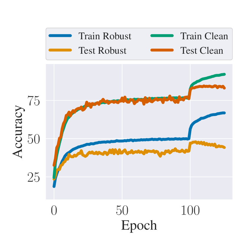
(a) PGD¹⁰ learning curves.

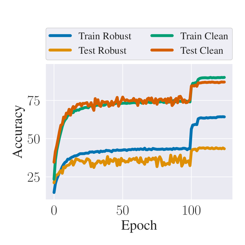
(b) BETA-AT¹⁰ learning curves.

Figure 1: BETA does not suffer from robust overfitting. We plot the learning curves against a PGD²⁰ adversary for PGD¹⁰ and BETA-AT¹⁰. Observe that although PGD displays robust overfitting after the first learning rate decay step, BETA-AT does not suffer from this pitfall.

In this section, we evaluate the performance of BETA and BETA-AT on CIFAR-10 [57]. Throughout, we consider a range of AT algorithms, including PGD [25], FGSM [26], TRADES [27], MART [31], as well as a range of adversarial attacks, including APGD and AutoAttack [41]. We consider the standard perturbation budget of $\epsilon=8/255$, and all training and test-time attacks use a step size of $\alpha=2/255$. For both TRADES and MART, we set the trade-off parameter $\lambda=5$, which is consistent with the original implementations [31, 27].

The bilevel formulation eliminates robust overfitting. Robust overfitting occurs when the robust test accuracy peaks immediately after the first learning rate decay, and then falls significantly in subsequent epochs as the model continues to train [39]. This is illustrated in Figure 1(a), in which we plot the learning curves (i.e., the clean and robust accuracies for the training and test sets) for a ResNet-18 [58] model trained using 10-step PGD against a 20-step PGD adversary. Notice that after the first learning rate decay step at epoch 100, the robust test accuracy spikes, before dropping off in subsequent epochs. On the other hand, BETA-AT does not suffer from robust overfitting, as shown in Figure 1(b). We argue that this strength of our method is a direct result of our bilevel formulation, in which we train against a proper surrogate for the adversarial classification error.

BETA-AT outperforms baselines on the last iterate of training. We next compare the performance of ResNet-18 models trained using four different AT algorithms: FGSM, PGD, TRADES, MART, and BETA. PGD, TRADES, and MART used a 10-step adversary at training time. At test time, the models were evaluated against five different adversaries: FGSM, 10-step PGD, 40-step PGD, 10-step BETA, and APGD. We report the performance of two different checkpoints for each algorithm: the best performing checkpoint chosen by early stopping on a held-out validation set, and the performance of the last checkpoint from training. Note that while BETA performs comparably to the baseline algorithms with respect to early stopping, it outperforms these algorithms significantly when the test-time adversaries attack the last checkpoint of training. This owes to the fact that BETA does not suffer from robust overfitting, meaning that the last and best checkpoints perform similarly.

Table 1: Adversarial performance on CIFAR-10. We report the test accuracies of various AT algorithms against different adversarial attacks on the CIFAR-10 dataset.

Training algorithm	Test accuracy
	Clean		FGSM		PGD10		PGD40		BETA10		APGD
	Best	Last	Best	Last	Best	Last	Best	Last	Best	Last	Best	Last
FGSM	81.96	75.43	94.26	94.22	42.64	1.49	42.66	1.62	40.30	0.04	41.56	0.00
PGD10	83.71	83.21	51.98	47.39	46.74	39.90	45.91	39.45	43.64	40.21	44.36	42.62
TRADES10	81.64	81.42	52.40	51.31	47.85	42.31	47.76	42.92	44.31	40.97	43.34	41.33
MART10	78.80	77.20	53.84	53.73	49.08	41.12	48.41	41.55	44.81	41.22	45.00	42.90
BETA-AT5	87.02	86.67	51.22	51.10	44.02	43.22	43.94	42.56	42.62	42.61	41.44	41.02
BETA-AT10	85.37	85.30	51.42	51.11	45.67	45.39	45.22	45.00	44.54	44.36	44.32	44.12
BETA-AT20	82.11	81.72	54.01	53.99	49.96	48.67	49.20	48.70	46.91	45.90	45.27	45.25

BETA matches the robustness estimate of AutoAttack. AutoAttack is a state-of-the-art adversarial attack which is widely used to estimate the robustness of trained models on leaderboards such as RobustBench [32, 41]. In brief, AutoAttack comprises a collection of four disparate attacks: APGD-CE, APGD-T, FAB, and Square Attack. AutoAttack also involves several heuristics, including multiple restarts and variable stopping conditions. In Table 2, we compare the performance of the top-performing models on RobustBench against AutoAttack, APGD-T, and BETA with RMSprop. Both APGD-T and BETA used thirty steps, whereas we used the default implementation of AutoAttack, which runs for 100 iterations. We also recorded the gap between AutoAttack and BETA. Notice that the 30-step BETA—a heuristic-free algorithm derived from our bilevel formulation of AT—performs almost identically to AutoAttack, despite the fact that AutoAttack runs for significantly more iterations and uses five restarts, which endows AutoAttack with an unfair computational advantage. That is, excepting for a negligible number of samples, BETA matches the robustness estimate of AutoPGD-targeted and AutoAttack, despite using an off-the-shelf optimizer.

Table 2: Estimated $\ell_{\infty}$ robustness (robust test accuracy). BETA+RMSprop (ours) vs APGD-targeted (APGD-T) vs AutoAttack (AA). CIFAR-10. BETA and APGD-T use 30 iterations + single restart. $\epsilon=8/255$. AA uses 4 different attacks with 100 iterations and 5 restarts.

Model	BETA	APGD-T	AA	BETA/AA gap	Architecture
Wang et al. [59]	70.78	70.75	70.69	0.09	WRN-70-16
Wang et al. [59]	67.37	67.33	67.31	0.06	WRN-28-10
Rebuffi et al. [60]	66.75	66.71	66.58	0.17	WRN-70-16
Gowal et al. [61]	66.27	66.26	66.11	0.16	WRN-70-16
Huang et al. [62]	65.88	65.88	65.79	0.09	WRN-A4
Rebuffi et al. [60]	64.73	64.71	64.64	0.09	WRN-106-16
Rebuffi et al. [60]	64.36	64.27	64.25	0.11	WRN-70-16
Gowal et al. [61]	63.58	63.45	63.44	0.14	WRN-28-10
Pang et al. [63]	63.38	63.37	63.35	0.03	WRN-70-16

6 Related work

Robust overfitting. Several recent papers (see, e.g., [60, 64, 65, 66, 31, 67]) have attempted to explain and resolve robust overfitting [39]. However, none of these works point to a fundamental limitation of adversarial training as the cause of robust overfitting. Rather, much of this past work has focused on proposing heuristics for algorithms specifically designed to reduce robust overfitting, rather than to improve adversarial training. In contrast, we posit that the lack of guarantees of the zero-sum surrogate-based AT paradigm [25] is at fault, as this paradigm is not designed to maximize robustness with respect to classification error. And indeed, our empirical evaluations in the previous section confirm that our non-zero-sum formulation eliminates robust overfitting.

Estimating adversarial robustness. There is empirical evidence that attacks based on surrogates (e.g., PGD) overestimate the robustness of trained classifiers [41, 52, 55]. Indeed, this evidence served as motivation for the formulation of more sophisticated attacks like AutoAttack [41], which empirically tend to provide more accurate estimates of robustness. In contrast, we provide solid, theoretical evidence that commonly used attacks overestimate robustness due to the misalignment between standard surrogate losses and the adversarial classification error. Moreover, we show that optimizing the BETA objective with a standard optimizer (e.g., RMSprop) achieves the same robustness as AutoAttack without employing ad hoc training procedures such as multiple restarts. convoluted stopping conditions, or adaptive learning rates.

One notable feature of past work is an overservation made in [55], which finds that multitargeted attacks tend to more accurately estimate robustness. However, their theoretical analysis only applies to linear functions, whereas our work extends these ideas to the nonlinear setting of DNNs. Moreover, [55] do not explore training using a multitargeted attack, whereas we show that BETA-AT is an effective AT algorithm that mitigates the impact of robust overfitting.

Bilevel formulations of AT. Prior to our work, [68] proposed a different pseudo-bilevel formulation for AT, wherein the main objective was to justify the Fast AT algorithm introduced in [69]. More specifically, the formulation in [68] is designed to produce solutions that coincide with the iterates of Fast AT by linearizing the attacker’s objective. In contrast, our bilevel formulation appears naturally following principled relaxations of the intractable classification error AT formulation. In this way, the formulation in [68] applies only in the context of Fast AT, whereas our formulation deals more generally with the task of adversarial training.

7 Conclusion

In this paper, we rigorously studied the standard zero-sum formulation of adversarial training. We argued that the surrogate-based relaxation commonly employed to improve the tractability of this problem voids guarantees on the ultimate robustness of trained classifiers, resulting in weak adversaries and ineffective AT algorithms. This shortcoming motivated the formulation of a novel, yet natural bilevel approach to adversrial training and evaluation. In our paradigm, the adversary and defender optimize separate objectives, which constitutes a non-zero-sum game that preserves guarantees on robustness. Based on this formulation, we developed a new adversarial attack algorithm—BETA, which stands for BEst Adversarial Attack—and a concomitant AT algorithm, which we call BETA-AT. In our experiments, we showed that BETA-AT eliminates robust overfitting, which we argued is a direct result of optimizing an objective which is aligned with the goal of finding true adversarial examples. We also showed that even when early stopping based model selection is used, BETA-AT performed comparably to AT. And finally, we showed that BETA provides almost identical estimates of robustness to AutoAttack, indicating that when the adversarial objective closely matches the true objective, one need not resort to heuristics like multiple restarts, variable stopping conditions, and adaptive learning rate schedules to accurately estimate robustness.

With regard to the bilevel formulation in this paper, future directions abound. One could imagine applying this framework to other changes in the data space, including the kinds of distribution shifts that are common in fields like domain adaptation and domain generalization. A convergence analysis of BETA and an analysis of the sample complexity of BETA-AT are two more directions that we leave for future work. The prospect of applying more sophisticated bilevel optimization algorithmic techniques to this problem is also a promising avenue for future research.

Appendix A Proof of proposition 1

Suppose there exists $\hat{\eta}$ satisfying $\left|\left|\hat{\eta}\right|\right|\leq\epsilon$ such that for some $j\in[K]$, $j\neq Y$ we have $M_{\theta}(X+\hat{\eta},Y)_{j}>0$, i.e., assume

$$\max_{j\in[K]-\{Y\},\>\eta:\|\eta\|\leq\epsilon}M_{\theta}(X+\eta,Y)_{j}>0$$ (23)

for such $\hat{\eta}$ and such $j$ we have $f_{\theta}(X+\hat{\eta})_{j}>f_{\theta}(X+\hat{\eta})_{Y}$ and thus $\operatorname*{arg\,max}_{j\in[K]}f_{\theta}(X+\hat{\eta})_{j}\neq Y$. Hence, such $\hat{\eta}$ induces a misclassification error i.e.,

$$\hat{\eta}\in\operatorname*{arg\,max}_{\eta:\|\eta\|_{2}\leq\epsilon}\left\{\operatorname*{arg\,max}_{j\in[K]}f_{\theta}(X+\eta)_{j}\neq Y\right\}$$ (24)

In particular if

$$(j^{\star},\eta^{\star})\in\operatorname*{arg\,max}_{j\in[K]-\{Y\},\>\eta:\|\eta\|\leq\epsilon}M_{\theta}(X+\eta,Y)_{j}\Rightarrow\eta^{\star}\in\operatorname*{arg\,max}_{\eta:\|\eta\|_{2}\leq\epsilon}\left\{\operatorname*{arg\,max}_{j\in[K]}f_{\theta}(X+\eta)_{j}\neq Y\right\}$$ (25)

Otherwise, assume

$$\max_{j\in[K]-\{Y\},\>\eta:\|\eta\|\leq\epsilon}M_{\theta}(X+\eta,Y)_{j}<0,$$ (26)

then for all $\eta:\>\left|\left|\eta\right|\right|<\epsilon$ and all $j\neq Y$ we have $f_{\theta}(X+\eta)_{j}<f_{\theta}(X+\eta)_{Y}$, so that $\operatorname*{arg\,max}_{j\in[K]}f_{\theta}(x+\eta)_{j}=Y$ i.e., there is no adversarial example in the ball. In this case for any $\eta$, in particular In particular if

$$(j^{\star},\eta^{\star})\in\operatorname*{arg\,max}_{j\in[K]-\{Y\},\>\eta:\|\eta\|\leq\epsilon}M_{\theta}(X+\eta,Y)_{j}$$ (27)

Then

$$0=\left\{\operatorname*{arg\,max}_{j\in[K]}f_{\theta}(X+\eta^{\star})_{j}\neq Y\right\}=\max_{\eta:\|\eta\|_{2}\leq\epsilon}\left\{\operatorname*{arg\,max}_{j\in[K]}f_{\theta}(X+\eta)_{j}\neq Y\right\}$$ (28)

In conclusion, the solution

$$(j^{\star},\eta^{\star})\in\operatorname*{arg\,max}_{j\in[K]-\{Y\},\>\eta:\|\eta\|\leq\epsilon}M_{\theta}(X+\eta,Y)_{j}$$ (29)

always yields a maximizer of the misclassification error.

Appendix B Smooth reformulation of the lower level

First, note that the problem in eqs. 20, 21 and 22 is equivalent to

$$\begin{split}&\min_{\theta\in\Theta}\frac{1}{n}\sum_{i=1}^{n}\sum_{j=1}^{K}\lambda^{\star}_{ij}\ell(f_{\theta}(x_{i}+\eta^{\star}_{ij}),y_{i})\\ &\text{subject to }\lambda^{\star}_{ij},\eta^{\star}_{ij}\in\operatorname*{arg\,max}_{\begin{subarray}{c}\|\eta_{ij}\|\leq\epsilon\\ \lambda_{ij}\geq 0,\|\lambda_{i}\|_{1}=1,\lambda_{iy}=0\end{subarray}}\sum_{j=1}^{K}\lambda_{ij}M_{\theta}(x_{i}+\eta_{ij},y_{i})_{j}\qquad\forall i\in[n]\end{split}$$ (30)

This is because the maximum over $\lambda_{i}$ in eq. 30 is always attained at the coordinate vector $\mathbf{e}_{j}$ such that $M_{\theta}(x_{i}+\eta_{ij}^{\star},y_{i})$ is maximum.

An alternative is to smooth the lower level optimization problem by adding an entropy regularization:

$$\begin{split}\max_{\eta:\|\eta\|\leq\epsilon}\max_{j\in[K]-\{y\}}M_{\theta}(x+\eta_{j},y)_{j}&=\max_{\eta:\|\eta\|\leq\epsilon}\max_{\lambda\geq 0,\|\lambda\|_{1}=1,\lambda_{y}=0}\langle\lambda,M_{\theta}(x+\eta_{j},y)_{j=1}^{K}\rangle\\ &\geq\max_{\eta:\|\eta\|\leq\epsilon}\max_{\lambda\geq 0,\|\lambda\|_{1}=1,\lambda_{y}=0}\langle\lambda,M_{\theta}(x+\eta_{j},y)_{j=1}^{K}\rangle-\frac{1}{\mu}\sum_{j=1}^{K}\lambda_{j}\log(\lambda_{j})\\ &=\max_{\eta:\|\eta\|\leq\epsilon}\frac{1}{\mu}\log\left(\sum_{\begin{subarray}{c}j=1\\ j\neq y\end{subarray}}^{K}e^{\mu M_{\theta}(X+\eta,y)_{j}}\right)\end{split}$$ (31)

where $\mu>0$ is some temperature constant. The inequality here is due to the fact that the entropy of a discrete probability $\lambda$ is positive. The innermost maximization problem in (31) has the closed-form solution:

$$\lambda^{\star}_{j}=\frac{e^{\mu M_{\theta}(x+\eta_{j},y)_{j}}}{\sum_{\begin{subarray}{c}j=1\\ j\neq y\end{subarray}}^{K}e^{\mu M_{\theta}(x+\eta_{j},y)_{j}}}:j\neq y,\qquad\lambda^{\star}_{y}=0$$ (32)

Hence, after relaxing the second level maximization problem following eq. 31, and plugging in the optimal values for $\lambda$ we arrive at:

$$\begin{split}&\min_{\theta\in\Theta}\frac{1}{n}\sum_{i=1}^{n}\sum_{\begin{subarray}{c}j=1\\ j\neq y_{i}\end{subarray}}^{K}\frac{e^{\mu M_{\theta}(x_{i}+\eta_{ij},y_{i})_{j}}}{\sum_{\begin{subarray}{c}j=1\\ j\neq y_{i}\end{subarray}}^{K}e^{\mu M_{\theta}(x_{i}+\eta_{ij},y_{i})_{j}}}\ell(f_{\theta}(x_{i}+\eta^{\star}_{ij}),y_{i})\\ &\text{subject to }\eta^{\star}_{ij}\in\operatorname*{arg\,max}_{\|\eta_{ij}\|\leq\epsilon}M_{\theta}(x_{i}+\eta_{ij},y_{i})_{j}\qquad\forall i\in[n],j\in[K]\end{split}$$ (33)

$\displaystyle\min_{\theta\in\Theta}$ $\displaystyle\frac{1}{n}\sum_{i=1}^{n}\sum_{\begin{subarray}{c}j=1\\ j\neq y_{i}\end{subarray}}^{K}\frac{e^{\mu M_{\theta}(x_{i}+\eta^{\star}_{ij},y_{i})_{j}}}{\sum_{\begin{subarray}{c}j=1\\ j\neq y_{i}\end{subarray}}^{K}e^{\mu M_{\theta}(x_{i}+\eta^{\star}_{ij},y_{i})_{j}}}\ell(f_{\theta}(x_{i}+\eta^{\star}_{ij}),y_{i})$ (34) $\displaystyle\operatorname*{subject\,\,to\quad}$ $\displaystyle\eta^{\star}_{ij}\in\operatorname*{arg\,max}_{\eta:\|\eta\|\leq\epsilon}M_{\theta}(x_{i}+\eta,y_{i})_{j}$ $\displaystyle\forall i\in[n]$ (35)

In this formulation, both upper- and lower-level problems are smooth (barring the possible use of nonsmooth components like ReLU). Most importantly (I) the smoothing is obtained through a lower bound of the original objective in eqs. 21 and 22, retaining guarantees that the adversary will increase the misclassification error and (II) all the adversarial perturbations obtained for each class now appear in the upper level (34), weighted by their corresponding negative margin. In this way, we make efficient use of all perturbations generated: if two perturbations from different classes achieve the same negative margin, they will affect the upper-level objective in fair proportion. This formulation gives rise to algorithm 3.

Input: Dataset $(X,Y)=(x_{i},y_{i})_{i=1}^{n}$, perturbation size $\epsilon$, model $f_{\theta}$, number of classes $K$, iterations $T$, attack iterations $T^{\prime}$, temperature $\mu>0$

Output: Robust model $f_{\theta^{\star}}$

1 function $\text{SBETA-AT}{(}X,Y,\epsilon,\theta,T,\gamma,\mu{)}$

2       for $t\in 1,\ldots,T$ do

3             Sample $i\sim\text{Unif}[n]$

4             Initialize $\eta_{j}\sim\text{Unif}[\max(0,x_{i}-\epsilon),\min(x_{i}+\epsilon,1)],\forall j\in[K]$

5             for $j\in 1,\ldots,K$ do

6                   for $t\in 1,\ldots,T^{\prime}$ do

7                         $\eta_{j}\leftarrow\text{OPTIM}(\eta_{j},\nabla_{\eta}M_{\theta}(x_{i}+\eta_{j},y_{i})_{j})$ $\triangleright$ (attack optimizer step, e.g., RMSprop)

8                         $\eta_{j}\leftarrow\Pi_{B_{\epsilon}(x_{i})\cap[0,1]^{d}}(\eta_{j})$ $\triangleright$ (Projection onto valid perturbation set)

9                  

10            Compute $L(\theta)=\sum_{j=1,j\neq y_{i}}^{K}\frac{e^{\mu M_{\theta}(x_{i}+\eta_{j},y_{i})_{j}}}{\sum_{j=1,j\neq y_{i}}^{K}e^{\mu M_{\theta}(x_{i}+\eta_{j},y_{i})_{j}}}\ell(f_{\theta}(x_{i}+\eta_{j}),y_{i})$

11             $\theta\leftarrow\text{OPTIM}(\theta,\nabla L(\theta))$ $\triangleright$ (model optimizer step)

12      return $f_{\theta}$

13

Algorithm 3 Smooth BETA Adversarial Training (SBETA-AT)

References

- Robey et al. [2020] Alexander Robey, Hamed Hassani, and George J Pappas. Model-based robust deep learning: Generalizing to natural, out-of-distribution data. arXiv preprint arXiv:2005.10247, 2020.
- Laidlaw et al. [2020] Cassidy Laidlaw, Sahil Singla, and Soheil Feizi. Perceptual adversarial robustness: Defense against unseen threat models. arXiv preprint arXiv:2006.12655, 2020.
- Hendrycks and Dietterich [2019] Dan Hendrycks and Thomas Dietterich. Benchmarking neural network robustness to common corruptions and perturbations. In International Conference on Learning Representations, 2019.
- Hendrycks et al. [2021] Dan Hendrycks, Steven Basart, Norman Mu, Saurav Kadavath, Frank Wang, Evan Dorundo, Rahul Desai, Tyler Zhu, Samyak Parajuli, Mike Guo, et al. The many faces of robustness: A critical analysis of out-of-distribution generalization. In Proceedings of the IEEE/CVF International Conference on Computer Vision, pages 8340–8349, 2021.
- Eykholt et al. [2018] Kevin Eykholt, Ivan Evtimov, Earlence Fernandes, Bo Li, Amir Rahmati, Chaowei Xiao, Atul Prakash, Tadayoshi Kohno, and Dawn Song. Robust physical-world attacks on deep learning visual classification. In Proceedings of the IEEE conference on computer vision and pattern recognition, pages 1625–1634, 2018.
- Santurkar et al. [2021] Shibani Santurkar, Dimitris Tsipras, and Aleksander Madry. Breeds: Benchmarks for subpopulation shift. International Conference on Learning Representations, 2021.
- Sohoni et al. [2020] Nimit Sohoni, Jared Dunnmon, Geoffrey Angus, Albert Gu, and Christopher Ré. No subclass left behind: Fine-grained robustness in coarse-grained classification problems. Advances in Neural Information Processing Systems, 33:19339–19352, 2020.
- Koh et al. [2021] Pang Wei Koh, Shiori Sagawa, Henrik Marklund, Sang Michael Xie, Marvin Zhang, Akshay Balsubramani, Weihua Hu, Michihiro Yasunaga, Richard Lanas Phillips, Irena Gao, et al. Wilds: A benchmark of in-the-wild distribution shifts. In International Conference on Machine Learning, pages 5637–5664. PMLR, 2021.
- Zhou et al. [2022] Allan Zhou, Fahim Tajwar, Alexander Robey, Tom Knowles, George J Pappas, Hamed Hassani, and Chelsea Finn. Do deep networks transfer invariances across classes? arXiv preprint arXiv:2203.09739, 2022.
- Xiao et al. [2021] Kai Xiao, Logan Engstrom, Andrew Ilyas, and Aleksander Madry. Noise or signal: The role of image backgrounds in object recognition. International Conference on Machine Learning, 2021.
- Arjovsky et al. [2019] Martin Arjovsky, Léon Bottou, Ishaan Gulrajani, and David Lopez-Paz. Invariant risk minimization. arXiv preprint arXiv:1907.02893, 2019.
- Eastwood et al. [2022] Cian Eastwood, Alexander Robey, Shashank Singh, Julius Von Kügelgen, Hamed Hassani, George J Pappas, and Bernhard Schölkopf. Probable domain generalization via quantile risk minimization. arXiv preprint arXiv:2207.09944, 2022.
- Sagawa et al. [2020] Shiori Sagawa, Aditi Raghunathan, Pang Wei Koh, and Percy Liang. An investigation of why overparameterization exacerbates spurious correlations. In International Conference on Machine Learning, pages 8346–8356. PMLR, 2020.
- Robey et al. [2021a] Alexander Robey, George J Pappas, and Hamed Hassani. Model-based domain generalization. Advances in Neural Information Processing Systems, 34:20210–20229, 2021a.
- Szegedy et al. [2013] Christian Szegedy, Wojciech Zaremba, Ilya Sutskever, Dumitru Erhan Joan Bruna, Ian Goodfellow, and Rob Fergus. Intriguing properties of neural networks. In ICLR, 2013.
- Biggio et al. [2013a] B. Biggio, I. Corona, D. Maiorca, B. Nelson, N. Srndic, P. Laskov, G. Giacinto, and F. Roli. Evasion attacks against machine learning at test time. In ECML/PKKD, 2013a.
- Biggio et al. [2012] Battista Biggio, Blaine Nelson, and Pavel Laskov. Poisoning attacks against support vector machines. arXiv preprint arXiv:1206.6389, 2012.
- Carlini and Wagner [2017] Nicholas Carlini and David Wagner. Towards evaluating the robustness of neural networks. In 2017 ieee symposium on security and privacy (sp), pages 39–57. Ieee, 2017.
- Biggio et al. [2013b] Battista Biggio, Igino Corona, Davide Maiorca, Blaine Nelson, Nedim Šrndić, Pavel Laskov, Giorgio Giacinto, and Fabio Roli. Evasion attacks against machine learning at test time. In Machine Learning and Knowledge Discovery in Databases: European Conference, ECML PKDD 2013, Prague, Czech Republic, September 23-27, 2013, Proceedings, Part III 13, pages 387–402. Springer, 2013b.
- Huang et al. [2015] Ruitong Huang, Bing Xu, Dale Schuurmans, and Csaba Szepesvari. Learning with a strong adversary. ArXiv, abs/1511.03034, 2015.
- Wong and Kolter [2018] Eric Wong and Zico Kolter. Provable defenses against adversarial examples via the convex outer adversarial polytope. ICML, 2018.
- Kurakin et al. [2017] Alexey Kurakin, Ian Goodfellow, and Samy Bengio. Adversarial examples in the physical world. ICLR Workshop, 2017. URL https://openreview.net/forum?id=HJGU3Rodl.
- Robey et al. [2021b] Alexander Robey, Luiz Chamon, George J Pappas, Hamed Hassani, and Alejandro Ribeiro. Adversarial robustness with semi-infinite constrained learning. Advances in Neural Information Processing Systems, 34:6198–6215, 2021b.
- Sridhar et al. [2022] Kaustubh Sridhar, Oleg Sokolsky, Insup Lee, and James Weimer. Improving neural network robustness via persistency of excitation. In 2022 American Control Conference (ACC), pages 1521–1526. IEEE, 2022.
- Madry et al. [2018] Aleksander Madry, Aleksandar Makelov, Ludwig Schmidt, Dimitris Tsipras, and Adrian Vladu. Towards deep learning models resistant to adversarial attacks. In ICLR, 2018.
- Goodfellow et al. [2015] Ian J Goodfellow, Jonathon Shlens, and Christian Szegedy. Explaining and harnessing adversarial examples. In ICLR, 2015.
- Zhang et al. [2019] Hongyang Zhang, Yaodong Yu, Jiantao Jiao, Eric P. Xing, Laurent El Ghaoui, and Michael I. Jordan. Theoretically principled trade-off between robustness and accuracy. In ICML, 2019.
- Bartlett et al. [2006] Peter L Bartlett, Michael I Jordan, and Jon D McAuliffe. Convexity, classification, and risk bounds. Journal of the American Statistical Association, 101(473):138–156, 2006. doi: 10.1198/016214505000000907. URL https://doi.org/10.1198/016214505000000907.
- Shalev-Shwartz and Ben-David [2014] Shai Shalev-Shwartz and Shai Ben-David. Understanding machine learning: From theory to algorithms. Cambridge university press, 2014.
- Roux [2017] Nicolas Le Roux. Tighter bounds lead to improved classifiers. In International Conference on Learning Representations, 2017. URL https://openreview.net/forum?id=HyAbMKwxe.
- Wang et al. [2020] Yisen Wang, Difan Zou, Jinfeng Yi, James Bailey, Xingjun Ma, and Quanquan Gu. Improving adversarial robustness requires revisiting misclassified examples. ICLR, 2020.
- Croce et al. [2020a] Francesco Croce, Maksym Andriushchenko, Vikash Sehwag, Edoardo Debenedetti, Nicolas Flammarion, Mung Chiang, Prateek Mittal, and Matthias Hein. Robustbench: a standardized adversarial robustness benchmark. arXiv preprint arXiv:2010.09670, 2020a.
- Tsipras et al. [2019a] Dimitris Tsipras, Shibani Santurkar, Logan Engstrom, Alexander Turner, and Aleksander Madry. Robustness may be at odds with accuracy. In ICLR, 2019a.
- Dobriban et al. [2020] Edgar Dobriban, Hamed Hassani, David Hong, and Alexander Robey. Provable tradeoffs in adversarially robust classification. arXiv preprint arXiv:2006.05161, 2020.
- Javanmard et al. [2020] Adel Javanmard, Mahdi Soltanolkotabi, and Hamed Hassani. Precise tradeoffs in adversarial training for linear regression. In Conference on Learning Theory, pages 2034–2078. PMLR, 2020.
- Schmidt et al. [2018] Ludwig Schmidt, Shibani Santurkar, Dimitris Tsipras, Kunal Talwar, and Aleksander Madry. Adversarially robust generalization requires more data. Advances in neural information processing systems, 31, 2018.
- Chen et al. [2020] Lin Chen, Yifei Min, Mingrui Zhang, and Amin Karbasi. More data can expand the generalization gap between adversarially robust and standard models. In International Conference on Machine Learning, pages 1670–1680. PMLR, 2020.
- Stutz et al. [2019] David Stutz, Matthias Hein, and Bernt Schiele. Disentangling adversarial robustness and generalization. In Proceedings of the IEEE Conference on Computer Vision and Pattern Recognition, pages 6976–6987, 2019.
- Rice et al. [2020] Leslie Rice, Eric Wong, and J Zico Kolter. Overfitting in adversarially robust deep learning. In ICML, 2020.
- Carlini et al. [2019] Nicholas Carlini, Anish Athalye, Nicolas Papernot, Wieland Brendel, Jonas Rauber, Dimitris Tsipras, Ian Goodfellow, Aleksander Madry, and Alexey Kurakin. On evaluating adversarial robustness. arXiv preprint arXiv:1902.06705, 2019.
- Croce and Hein [2020] Francesco Croce and Matthias Hein. Reliable evaluation of adversarial robustness with an ensemble of diverse parameter-free attacks. In International conference on machine learning, pages 2206–2216. PMLR, 2020.
- Kannan et al. [2018] H. Kannan, A. Kurakin, and I. Goodfellow. Adversarial logit pairing. arXiv preprint arXiv:1803.06373, 2018.
- Chan et al. [2020] Alvin Chan, Yi Tay, Yew Soon Ong, and Jie Fu. Jacobian adversarially regularized networks for robustness. ICLR, 2020.
- Hoffman et al. [2019] Judy Hoffman, Daniel A Roberts, and Sho Yaida. Robust learning with jacobian regularization. arXiv preprint arXiv:1908.02729, 2019.
- Finlay et al. [2018] Chris Finlay, Jeff Calder, Bilal Abbasi, and Adam Oberman. Lipschitz regularized deep neural networks generalize and are adversarially robust. arXiv preprint arXiv:1808.09540, 2018.
- Wu et al. [2020] Dongxian Wu, Shu tao Xia, and Yisen Wang. Adversarial weight perturbation helps robust generalization. NeurIPS, 2020.
- Sun et al. [2021] Xu Sun, Zhiyuan Zhang, Xuancheng Ren, Ruixuan Luo, and Liangyou Li. Exploring the vulnerability of deep neural networks: A study of parameter corruption. In Proceedings of the AAAI Conference on Artificial Intelligence, volume 35, pages 11648–11656, 2021.
- Foret et al. [2020] Pierre Foret, Ariel Kleiner, Hossein Mobahi, and Behnam Neyshabur. Sharpness-aware minimization for efficiently improving generalization. arXiv preprint arXiv:2010.01412, 2020.
- Latorre et al. [2023] Fabian Latorre, Igor Krawczuk, Leello Tadesse Dadi, Thomas Pethick, and Volkan Cevher. Finding actual descent directions for adversarial training. In The Eleventh International Conference on Learning Representations, 2023. URL https://openreview.net/forum?id=I3HCE7Ro78H.
- Bard [2013] Jonathan F Bard. Practical bilevel optimization: algorithms and applications, volume 30. Springer Science & Business Media, 2013.
- Mosbach et al. [2018] Marius Mosbach, Maksym Andriushchenko, Thomas Trost, Matthias Hein, and Dietrich Klakow. Logit pairing methods can fool gradient-based attacks. arXiv preprint arXiv:1810.12042, 2018.
- Croce et al. [2020b] Francesco Croce, Jonas Rauber, and Matthias Hein. Scaling up the randomized gradient-free adversarial attack reveals overestimation of robustness using established attacks. International Journal of Computer Vision, 128:1028–1046, 2020b.
- Tsipras et al. [2019b] D. Tsipras, S. Santurkar, L. Engstrom, A. Turner, and A. Madry. Robustness may be at odds with accuracy. In ICLR, 2019b.
- Robey et al. [2022] Alexander Robey, Luiz Chamon, George J Pappas, and Hamed Hassani. Probabilistically robust learning: Balancing average and worst-case performance. In International Conference on Machine Learning, pages 18667–18686. PMLR, 2022.
- Gowal et al. [2019] Sven Gowal, Jonathan Uesato, Chongli Qin, Po-Sen Huang, Timothy Mann, and Pushmeet Kohli. An alternative surrogate loss for pgd-based adversarial testing. arXiv preprint arXiv:1910.09338, 2019.
- Kingma and Ba [2014] Diederik P Kingma and Jimmy Ba. Adam: A method for stochastic optimization. arXiv preprint arXiv:1412.6980, 2014.
- Krizhevsky et al. [2009] Alex Krizhevsky, Vinod Nair, and Geoffrey Hinton. Cifar datasets (canadian institute for advanced research). 2009. URL http://www.cs.toronto.edu/~kriz/cifar.html.
- He et al. [2016] Kaiming He, Xiangyu Zhang, Shaoqing Ren, and Jian Sun. Deep residual learning for image recognition. In CVPR, 2016.
- Wang et al. [2023] Zekai Wang, Tianyu Pang, Chao Du, Min Lin, Weiwei Liu, and Shuicheng Yan. Better diffusion models further improve adversarial training. arXiv preprint arXiv:2302.04638, 2023.
- Rebuffi et al. [2021] Sylvestre-Alvise Rebuffi, Sven Gowal, Dan A. Calian, Florian Stimberg, Olivia Wiles, and Timothy Mann. Fixing data augmentation to improve adversarial robustness. arXiv preprint arXiv:2103.01946, 2021.
- Gowal et al. [2021] Sven Gowal, Sylvestre-Alvise Rebuffi, Olivia Wiles, Florian Stimberg, Dan Andrei Calian, and Timothy Mann. Improving robustness using generated data. In A. Beygelzimer, Y. Dauphin, P. Liang, and J. Wortman Vaughan, editors, Advances in Neural Information Processing Systems, 2021. URL https://openreview.net/forum?id=0NXUSlb6oEu.
- Huang et al. [2022] Shihua Huang, Zhichao Lu, Kalyanmoy Deb, and Vishnu Naresh Boddeti. Revisiting Residual Networks for Adversarial Robustness: An Architectural Perspective. arXiv e-prints, art. arXiv:2212.11005, December 2022. doi: 10.48550/arXiv.2212.11005.
- Pang et al. [2022] Tianyu Pang, Min Lin, Xiao Yang, Jun Zhu, and Shuicheng Yan. Robustness and accuracy could be reconcilable by (Proper) definition. In Kamalika Chaudhuri, Stefanie Jegelka, Le Song, Csaba Szepesvari, Gang Niu, and Sivan Sabato, editors, Proceedings of the 39th International Conference on Machine Learning, volume 162 of Proceedings of Machine Learning Research, pages 17258–17277. PMLR, 17–23 Jul 2022. URL https://proceedings.mlr.press/v162/pang22a.html.
- Chen et al. [2021] Tianlong Chen, Zhenyu Zhang, Sijia Liu, Shiyu Chang, and Zhangyang Wang. Robust overfitting may be mitigated by properly learned smoothening. In International Conference on Learning Representations, 2021. URL https://openreview.net/forum?id=qZzy5urZw9.
- Yu et al. [2022] Chaojian Yu, Bo Han, Li Shen, Jun Yu, Chen Gong, Mingming Gong, and Tongliang Liu. Understanding robust overfitting of adversarial training and beyond. In Kamalika Chaudhuri, Stefanie Jegelka, Le Song, Csaba Szepesvari, Gang Niu, and Sivan Sabato, editors, Proceedings of the 39th International Conference on Machine Learning, volume 162 of Proceedings of Machine Learning Research, pages 25595–25610. PMLR, 17–23 Jul 2022. URL https://proceedings.mlr.press/v162/yu22b.html.
- Dong et al. [2022] Yinpeng Dong, Ke Xu, Xiao Yang, Tianyu Pang, Zhijie Deng, Hang Su, and Jun Zhu. Exploring memorization in adversarial training. In International Conference on Learning Representations, 2022. URL https://openreview.net/forum?id=7gE9V9GBZaI.
- Lee et al. [2020] Saehyung Lee, Hyungyu Lee, and Sungroh Yoon. Adversarial vertex mixup: Toward better adversarially robust generalization. In Proceedings of the IEEE/CVF Conference on Computer Vision and Pattern Recognition (CVPR), June 2020.
- Zhang et al. [2022] Yihua Zhang, Guanhua Zhang, Prashant Khanduri, Mingyi Hong, Shiyu Chang, and Sijia Liu. Revisiting and advancing fast adversarial training through the lens of bi-level optimization. In Kamalika Chaudhuri, Stefanie Jegelka, Le Song, Csaba Szepesvari, Gang Niu, and Sivan Sabato, editors, Proceedings of the 39th International Conference on Machine Learning, volume 162 of Proceedings of Machine Learning Research, pages 26693–26712. PMLR, 17–23 Jul 2022. URL https://proceedings.mlr.press/v162/zhang22ak.html.
- Wong et al. [2020] Eric Wong, Leslie Rice, and J. Zico Kolter. Fast is better than free: Revisiting adversarial training. ICLR, 2020.