FP-IRL: Fokker-Planck-based Inverse Reinforcement Learning — A Physics-Constrained Approach to Markov Decision Processes

Abstract

Inverse Reinforcement Learning (IRL) is a compelling technique for revealing the rationale underlying the behavior of autonomous agents. IRL seeks to estimate the unknown reward function of a Markov decision process (MDP) from observed agent trajectories. However, IRL needs a transition function, and most algorithms assume it is known or can be estimated in advance from data. It therefore becomes even more challenging when such transition dynamics is not known a-priori, since it enters the estimation of the policy in addition to determining the system’s evolution. When the dynamics of these agents in the state-action space is described by stochastic differential equations (SDE) in Itô calculus, these transitions can be inferred from the mean-field theory described by the Fokker-Planck (FP) equation. We conjecture there exists an isomorphism between the time-discrete FP and MDP that extends beyond the minimization of free energy (in FP) and maximization of the reward (in MDP). We identify specific manifestations of this isomorphism and use them to create a novel physics-aware IRL algorithm, FP-IRL, which can simultaneously infer the transition and reward functions using only observed trajectories. We employ variational system identification to infer the potential function in FP, which consequently allows the evaluation of reward, transition, and policy by leveraging the conjecture. We demonstrate the effectiveness of FP-IRL by applying it to a synthetic benchmark and a biological problem of cancer cell dynamics, where the transition function is inaccessible.

1 Introduction

Principles may be unavailable for deciphering the incentive mechanism in a complex decision-making system, especially when we have poor or even no knowledge about the system (e.g., on the environment, agents, etc.). Important examples of this type arise in cancer biology where the mechanisms of cancer cell metastasis remain to be understood, and in human interactions where human agents may change unpredictably and into regimes not encountered previously. The stochasticity of the system and the heterogeneity among individuals (cells or humans) further complicate the problem. Nonetheless, learning incentives holds great potential for understanding these complex systems and eventually developing targeted interventions to control them. Inverse Reinforcement Learning (IRL) [25, 21, 23, 22, 32, 8] is a powerful tool that can aid in the data-driven recovery of incentive mechanisms that force the behavior of the target agent.

IRL has demonstrated remarkable success in diverse fields, such as human behaviors [23, 32], robotics [16], and biology [18]. However, it is not without limitations. Firstly, IRL typically requires a known mathematical model that represents the environment. This can be problematic in situations where knowledge about the environment dynamics is lacking or imperfect, and an explicit, analytical form of transition function is not available. The examples of interactions between cancer cells or human agents also fall under this category. An empirical treatment of transition functions can be undesirable because it is often very challenging to generalize to state and action regions away from training samples relying on observations alone, especially under high-dimensional settings and when training data is limited and noisy. Secondly, recent IRL algorithms with unknown transitions make rely on deep learning techniques [15]. However, the lack of interpretability in deep learning models can translate to a similar shortfall in credibility, both of which are of central importance in scientific applications.

With the above motivation, we propose a new method of physics-constrained IRL. This method simultaneously estimates the transition and reward functions using only data on trajectories, while also inferring physical principles that govern the system and using them to constrain the learning. The key contributions of our work center around a conjecture on the structural isomorphism between the physics governed by a well-known optimal transport model—the Fokker-Planck (FP) equation—and Markov Decision Processes (MDPs). This is arrived from leveraging fundamental principles of the FP physics to build models for the MDP. We then exploit these theoretical and modeling insights and propose the physics-based FP-IRL algorithm. Finally, we demonstrate FP-IRL through numerical experiments on synthetic and real-world examples.

2 Related Work

Studies most closely related to our work are as follows. Herman et al. [15] introduced a data-driven IRL to simultaneously estimate the reward and transition using neural networks, but devoid of physics. Garg et al. [9] proposed an IRL algorithm that learns the state-action value function first with a given transition, and infers the reward function using the inverse Bellman operator. Lastly, Kalantari et al. [20] applied a variant of Bayesian IRL to study gene mutations in cancer cell populations. In contrast to these, our framework will infer the transition and reward simultaneously but constrained by the FP physics, while exploiting the inverse Bellman operator in applications to study the migration dynamics of agents such as cancer cells and human actors. Besides these references, we briefly review other topics more broadly connected to our approach.

Inverse Reinforcement Learning (IRL) [25, 21] has the main goal of learning an unknown reward function. Many new IRL variants and extensions have since been developed. The maximum margin method [21, 23] infers a reward function such that the expected reward of the demonstrated policy exceeds that of other sub-optimal policies by a maximal margin. The reward function inferred by the feature matching method [1] maximizes the margin while driving the resulting policy to be close to the demonstrated policy by comparing their feature counts. Entropy regularization has been added to feature matching to represent the uncertainty of predictions in [32, 31, 30]. Using generative imitation learning [16], adversarial IRL [8, 29, 14] has extended entropy-regularized IRL to generative adversarial modeling [10]. Finally, Bayesian IRL [22, 20] computes the likelihood of trajectories given a reward function and uses Bayesian inference to quantify the uncertainty surrounding the reward function.

Entropy Regularized Reinforcement Learning (also called soft reinforcement learning or energy-based reinforcement learning) uses the principle of maximum entropy to regularize reward inference [31] in order to obtain a robust optimal policy in an uncertain environment [3, 11, 12, 13]. The objective function bears a formal similarity to the free energy in statistical physics, but does not have the rigorous connection to it that we establish in this work.

Free Energy Principle [7, 4, 5] propose a general principle that defines a free energy related to information-theoretic ideas. When extended to reinforcement learning [6], the information gain in this setting can be interpreted as the reward.

3 Fokker-Planck-based Inverse Reinforcement Learning

In this section, we introduce the fundamentals of MDP and discuss the modeling of an MDP using FP in the IRL context. We then conjecture a structure isomorphism between the MDP and FP, and discuss the method to estimate the transition, reward, and policy leveraging the conjecture.

3.1 Preliminaries

3.1.1 Markov Decision Processes and Reinforcement Learning

A Markov Decision Process (MDP) is defined by a tuple $\mathcal{M}\triangleq\{\mathcal{S},\mathcal{A},p_{0}(\cdot),R(\cdot),T(\cdot)\}$ consisting of a state space $\mathcal{S}$ with possible states $\boldsymbol{s}\in\mathcal{S}$, action space $\mathcal{A}$ with possible actions $\boldsymbol{a}\in\mathcal{A}$, initial state probability function $p_{0}(\boldsymbol{s}):\mathcal{S}\mapsto\mathbb{P}$, reward function $R(\boldsymbol{s},\boldsymbol{a}):\mathcal{S}\times\mathcal{A}\mapsto\mathbb{R}$ that evaluates the instantaneous scalar reward when taking action $\boldsymbol{a}$ at state $\boldsymbol{s}$, and transition probability function $T(\boldsymbol{s}^{\prime}|\boldsymbol{s},\boldsymbol{a}):\mathcal{S}\times\mathcal{A}\times\mathcal{S}\mapsto\mathbb{P}$ that evaluates the probability of transitioning to state $\boldsymbol{s}^{\prime}$ when taking action $\boldsymbol{a}$ at state $\boldsymbol{s}$.

In infinite-horizon MDP, Reinforcement Learning (RL) is concerned with finding a time-invariant (stochastic) policy $\pi(\boldsymbol{a}|\boldsymbol{s}):\mathcal{S}\times\mathcal{A}\mapsto\mathbb{P}$ (evaluating the probability of taking action $\boldsymbol{a}$ at state $\boldsymbol{s}$) that maximizes the expected cumulative discounted reward:

$$\pi^{*}(\cdot)=\operatorname*{arg\,max}_{\pi(\cdot)\in\Pi}\quad\mathbb{E}_{\begin{subarray}{c}\boldsymbol{s}_{0}\sim p_{0}(\cdot),\\ \boldsymbol{a}_{t}\sim\pi(\cdot|\boldsymbol{s}_{t}),\\ \boldsymbol{s}_{t+1}\sim T(\cdot|\boldsymbol{s}_{t},\boldsymbol{a}_{t})\end{subarray}}\left[\sum_{t=0}^{\infty}\gamma^{t}R(\boldsymbol{s}_{t},\boldsymbol{a}_{t})\right].$$ (1)

where $\gamma\in[0,1)$ is the future reward discount factor. The expected cumulative reward can also be written in recursive form, and the RL problem is equivalent to finding a policy maximizing the Bellman expectation equations [2]:

$$Q_{\pi}(\boldsymbol{s},\boldsymbol{a})= R(\boldsymbol{s},\boldsymbol{a})+\gamma\mathbb{E}_{\boldsymbol{s}^{\prime}\sim T(\cdot|\boldsymbol{s},\boldsymbol{a})}\left[V_{\pi}(\boldsymbol{s}^{\prime})\right]$$ (2a)

$$V_{\pi}(\boldsymbol{s})= \mathbb{E}_{\boldsymbol{a}\sim\pi(\cdot|\boldsymbol{s})}\left[Q_{\pi}(\boldsymbol{s},\boldsymbol{a})\right],$$ (2b)

where $Q(\boldsymbol{s},\boldsymbol{a})$ is the state-action value function that evaluates the expected cumulative rewards when choosing action $\boldsymbol{a}$ at state $\boldsymbol{s}$, and $V(\boldsymbol{s})$ is the state-value function that evaluates the expected cumulative rewards if the agent is at state $\boldsymbol{s}$.

3.1.2 Inverse Reinforcement Learning

Inverse Reinforcement Learning (IRL) is a problem where the goal is to infer unknown reward function $R(\cdot)$ from observed trajectories $\mathcal{D}\triangleq\{(\boldsymbol{s}_{0}^{(i)},\boldsymbol{a}_{0}^{(i)},\cdots,\boldsymbol{s}_{\tau_{i}}^{(i)},\boldsymbol{a}_{\tau_{i}}^{(i)}))\}_{i=1}^{N}$ ($N$ denotes the number of trajectories, $\tau_{i}$ the number of timesteps in the $i$-th trajectory) of a demonstrator (e.g., expert) who employs a policy that maximizes the unknown expected rewards. Thus, the reward function encapsulates the incentive mechanism and quantifies the motivation of the agent’s behavior.

Conventionally, only $R(\cdot)$ is unknown from the MDP while all other components, including the transition probability function $T(\cdot)$, are assumed known or given. The transition is crucial to enable trajectory sampling, allowing the IRL problem to be tackled iteratively by adjusting the proposed $R(\cdot)$ so that the difference between simulated and observed trajectories can be minimized. However, in many real-life problems $T(\cdot)$ is also unknown (e.g., a probabilistic rule for cancer cell migration is not available). The absence of $T(\cdot)$ thus introduces indeterminacy, allowing many more transition-reward pairings to potentially describe the demonstrator behavior. It is then crucial to combat this exacerbated ill-posedness by introducing additional regularization and constraints. We propose to achieve this by incorporating physical principles into IRL that will yield physically-meaningful and explainable results, instead of employing pure data-driven black-box models [15] for learning the transition and reward functions.

3.2 Physics-based Modeling for Learning the Transition Function

The FP equation arises in many contexts in physics wherein the time evolution of a density function can be posed as an optimal transport map. It therefore provides a framework to model physical systems of evolving distributions, and motivates our strategy to inject physics into IRL by constraining and learning the transition of the probability density function through the FP dynamics. This is achieved by first recognizing that an MDP with a given policy $\pi(\cdot)$ reduces to a Markov process (MP) on the lumped state $\boldsymbol{x}=(\boldsymbol{s},\boldsymbol{a})$, where the MP transition is

$$T_{\text{MP}}(\boldsymbol{x}^{\prime}|\boldsymbol{x})=T_{\text{MP}}(\boldsymbol{s}^{\prime},\boldsymbol{a}^{\prime}|\boldsymbol{s},\boldsymbol{a})=\pi(\boldsymbol{a}^{\prime}|\boldsymbol{s}^{\prime})T(\boldsymbol{s}^{\prime}|\boldsymbol{s},\boldsymbol{a})$$ (3)

with $\pi(\boldsymbol{a}^{\prime}|\boldsymbol{s}^{\prime})=\pi(\boldsymbol{a}^{\prime}|\boldsymbol{s}^{\prime},\boldsymbol{s},\boldsymbol{a})$ due to the Markov property. Then, if the MP joint transition can be inferred, we would also be able to retrieve the MDP transition via

$$T(\boldsymbol{s}^{\prime}|\boldsymbol{s},\boldsymbol{a})=\int_{\mathcal{A}}T_{\text{MP}}(\boldsymbol{s}^{\prime},\boldsymbol{a}^{\prime}|\boldsymbol{s},\boldsymbol{a})\ d\boldsymbol{a}^{\prime}.$$ (4)

Learning the MP transition will leverage connections between MPs and stochastic differential equations (SDEs). Specifically, we target the class of stochastic processes whose dynamics are governed by the Itô SDE (e.g., FP dynamics):

$$\mathrm{d}\boldsymbol{X}(t)=-\nabla\psi(\boldsymbol{X}(t))\mathrm{d}t+\sqrt{2\beta^{-1}}\mathrm{d}\boldsymbol{W}(t)$$ (5)

where $\boldsymbol{X}$ denotes the lumped state random variable of dimension $d$, $\psi(\cdot)$ is the potential function, $\beta$ is the inverse temperature in statistical physics, and $\boldsymbol{W}$ is a $d$-dimensional Wiener process. Thus, the change of state involves directed motion down a potential gradient and diffusion resulting in a random walk from the Wiener process. Under finite time step $\Delta t$, the state transition for this SDE follows a Gaussian distribution:

$$T_{\text{MP}}(\boldsymbol{x}^{\prime}|\boldsymbol{x})=\left(\frac{\beta}{4\pi\Delta t}\right)^{d/2}\exp{\left(\frac{-\beta||\boldsymbol{x}-\boldsymbol{x}^{\prime}-\nabla\psi(\boldsymbol{x})\Delta t||^{2}}{4\Delta t}\right)}.$$ (6)

Fully describing the MP transition thus requires $\psi(\cdot)$ and $\beta$. We approach this learning task by enlisting the FP partial differential equation (PDE) [24] that correspondingly describes the evolution of probability density of states $p(\boldsymbol{x})$ under the Itô SDE in Eq. 5:

$$\frac{\partial p}{\partial t}=\nabla\cdot(\nabla\psi(\boldsymbol{x})p)+\beta^{-1}\Delta p.$$ (7)

As we show below LABEL:{sec:vsi}, the form of the FP PDE Eq. 7 can be inferred from data $\mathcal{D}$ using an approach called Variational System Identification (VSI).

3.3 Free Energy in an MDP System

Once the MDP transition is obtained, the remaining task for IRL entails estimating the reward function and corresponding optimal policy. This is enabled by a key conjecture of this work, that the value function in MDP is equivalent to the potential function in FP of MDP-induced MP by using free energy functional.

In statistical mechanics, free energy plays a central role in understanding the behavior of physical systems as it allows us to calculate the equilibrium properties and predict the outcomes of (thermodynamic) processes. Free energy $F$ is defined to be a function of internal energy and entropy of a stochastic system:

$$F(p)= \int_{\mathcal{X}}\psi(\boldsymbol{x})p(\boldsymbol{x})d\boldsymbol{x}+\beta^{-1}\int_{\mathcal{X}}p(\boldsymbol{x})\log p(\boldsymbol{x})d\boldsymbol{x}.$$ (8)

The principle of minimum free energy states that a system will evolve towards a state of minimum $F$ (i.e. maximum stability). Jordan et al. [19] further proved that the solution of

$$p_{t+1}=\operatorname*{arg\,min}_{p}W_{2}(p_{t},p)^{2}+\Delta t\ F(p)$$ (9)

converges to the solution of FP PDE in Eq. 7 as $\Delta t\to 0$, where $W_{2}(\cdot,\cdot)$ denotes the Wasserstein-2 distance between two distributions. The Wasserstein flows are thus generated by minimizing $F(p)$ in an isomorphism to the maximization of the cumulative reward, or value, in MDPs.

In an MDP system, the agent’s policy is designed to maximize the value function while being constrained by the environment’s dynamics (transition function). This means that the agent employs its policy to reach states where the value function is high. We can also observe that in the context of a population of agents in the MDP or in the probability view of the agent states, the expected value function ($\mathbb{E}_{p_{t}(\boldsymbol{s},\boldsymbol{a})}[Q(\boldsymbol{s},\boldsymbol{a})]$ or $\mathbb{E}_{p_{t}(\boldsymbol{s})}[V(\boldsymbol{s})]$) will increase over time $t$ while being constrained by the environment’s dynamics. The system satisfies the principle of minimum energy. Therefore, we propose the following conjecture.

Conjecture 3.1.

The potential function in FP is equivalent to the negative state-action value function in MDP:

$$\psi(\boldsymbol{s},\boldsymbol{a})=-Q_{\pi}(\boldsymbol{s},\boldsymbol{a}).$$ (10)

Remark.

The potential function is the driver whose minimization leads to FP dynamics. The value function is the driver whose maximization leads to the MDP. This equivalence thus leads to the isomorphism between FP dynamics and the MDP. ∎

In an MDP, the minimization of free energy can be achieved in two ways. (1) At any given state distribution over time, the agent can minimize the free energy by finding an optimal policy, so that the potential function is optimal and drives the state distribution towards lower free energy (high expected reward). Because the policy is not fully determined by the other components of an MDP, any arbitrary policy will have its own value function by the Contraction Mapping Theorem. In order to reduce the free energy in the global sense, the policy should be optimal, and therefore, the value function should be maximized. (2) If the policy is already optimal and fixed, applying it repeatedly over time will lead to the free energy minimum of the system. Because in IRL, we assume the agent already adopts an optimal policy, case (1) above is not considered in our model, but gives us a fundamental reason for why the value function is equivalent to the (negative) FP potential function.

3.4 The Agent’s Policy Constrained by FP

In this section, we show that the Boltzmann policy is the optimal policy when constrained by FP physics.

The steady-state distribution $p_{\infty}(\boldsymbol{x})$ of the Fokker-Planck dynamics minimizes the free energy functional, and has the form of the Gibbs-Boltzmann density [19].

$$p_{\infty}(\boldsymbol{x})=p_{\infty}(\boldsymbol{s},\boldsymbol{a})=Z^{-1}\exp(-\beta\psi(\boldsymbol{s},\boldsymbol{a}))$$ (11)

where $Z=\int_{\mathcal{S}}\int_{\mathcal{A}}\exp(-\beta\psi(\boldsymbol{s},\boldsymbol{a}))\mathrm{d}\boldsymbol{a}\mathrm{d}\boldsymbol{s}$ is a normalization constant. The marginalized steady-state distribution of state $\boldsymbol{s}$ follows:

$$p_{\infty}(\boldsymbol{s})=\int_{\mathcal{A}}p_{\infty}(\boldsymbol{s},\boldsymbol{a})\mathrm{d}\boldsymbol{a}=Z^{-1}\int_{\mathcal{A}}\exp(-\beta\psi(\boldsymbol{s},\boldsymbol{a}))d\boldsymbol{a}.$$ (12)

Therefore, the conditional distribution of action $\boldsymbol{a}$ given state $\boldsymbol{s}$ is

$$p_{\infty}(\boldsymbol{a}|\boldsymbol{s})=\frac{p_{\infty}(\boldsymbol{s},\boldsymbol{a})}{p_{\infty}(\boldsymbol{s})}=\frac{\exp(-\beta\psi(\boldsymbol{s},\boldsymbol{a}))}{\int_{\mathcal{A}}\exp(-\beta\psi(\boldsymbol{s},\boldsymbol{a}^{\prime}))d\boldsymbol{a}^{\prime}}$$ (13)

which is in the same form as the Boltzmann policy Eq. 14 in the previous RL study [26, 31, 12, 13].

$$\pi^{*}(\boldsymbol{a}|\boldsymbol{s})=\frac{\exp(\beta Q_{\pi}(\boldsymbol{s},\boldsymbol{a}))}{\int_{\mathcal{A}}\exp(\beta Q_{\pi}(\boldsymbol{s},\boldsymbol{\hat{a}}))d\boldsymbol{\hat{a}}}$$ (14)

Thus providing some evidence for our 3.1.

In Sec. 3.2, we have shown that the MDP reduces to an MP when the policy is fixed. Now, we expand the MP back to an MDP. For lumped state $\boldsymbol{x}$, the transformation of $p(\boldsymbol{s})$ to $p(\boldsymbol{s},\boldsymbol{a})$ happens through the optimal policy, which follows the Boltzmann distribution. While the optimal policy has been identified as Boltzmann in the steady state, a reasonable assumption is that this result holds also in the transient state, as it is consistent with the conclusion of the time-invariant policy in the MDP.

The Wasserstein distance, $W_{2}(p_{t},p)^{2}$ in Eq. 9 appears in a form known as a movement-limiter. It imposes a physics constraint that the change in the distribution should be small in an infinitesimal time step. Thus it can be neglected in the context of the MDP and the minimization problem in Eq. 9 for an agent becomes

$$\pi^{\ast}=\operatorname*{arg\,min}_{\pi(\cdot|\cdot)}F(p,\pi,-Q_{\pi})$$ (15)

where

$$\begin{split}F(p,\pi,-Q_{\pi})=&-\int_{\mathcal{S}}\int_{\mathcal{A}}p(\boldsymbol{s},\boldsymbol{a})Q_{\pi}(\boldsymbol{s},\boldsymbol{a})\mathrm{d}\boldsymbol{a}\ \mathrm{d}\boldsymbol{s}+\beta^{-1}\int_{\mathcal{S}}\int_{\mathcal{A}}p(\boldsymbol{s},\boldsymbol{a})\log p(\boldsymbol{s},\boldsymbol{a})\mathrm{d}\boldsymbol{a}\ \mathrm{d}\boldsymbol{s}\end{split}$$ (16)

$$\begin{split}=&\int_{\mathcal{S}}p(\boldsymbol{s})\int_{\mathcal{A}}\pi(\boldsymbol{a}|\boldsymbol{s})\left[-Q_{\pi}(\boldsymbol{s},\boldsymbol{a})+\beta^{-1}\log\pi(\boldsymbol{a}|\boldsymbol{s})\right]\mathrm{d}\boldsymbol{a}\mathrm{d}\boldsymbol{s}\end{split}$$ (17)

Because $p(\boldsymbol{s})$ is transitioned from the previous time step by environment and cannot be optimized, the optimal policy for a given value function is the Boltzmann policy for a given value function, by substituting Eq. 17 into Eq. 15.

3.5 Inverse Bellman Equation

With the transition function Eq. 4 of the induced Markov process and state-action value function $Q_{\pi}(\boldsymbol{s},\boldsymbol{a})$ obtained from Fokker-Planck equation 3.1 and Boltzmann policy Eq. 14, the reward function $R(\cdot)$ can be simply derived from the inverse Bellman equation

$$R(\boldsymbol{s},\boldsymbol{a})=Q_{\pi}(\boldsymbol{s},\boldsymbol{a})-\gamma\mathbb{E}_{\boldsymbol{s}^{\prime},\boldsymbol{a}^{\prime}\sim T(\cdot|\boldsymbol{s},\boldsymbol{a})}\left[Q_{\pi}(\boldsymbol{s}^{\prime},\boldsymbol{a}^{\prime})\right].$$ (18)

Thus, there is a unique reward function Eq. 18 corresponding to a pair of transition and value functions as shown in Theorem 3.2.

Theorem 3.2.

Define the inverse Bellman operator $\mathcal{T}:\mathcal{Q}\mapsto\mathcal{R}$ (where $\mathcal{Q},\mathcal{R}$ denote the spaces of value functions and reward functions, respectively) such that

$$(\mathcal{T}Q_{\pi})(\boldsymbol{s},\boldsymbol{a})=Q_{\pi}(\boldsymbol{s},\boldsymbol{a})-\gamma\mathbb{E}_{\boldsymbol{s}^{\prime},\boldsymbol{a}^{\prime}\sim T(\cdot|\boldsymbol{s},\boldsymbol{a})}\left[Q_{\pi}(\boldsymbol{s}^{\prime},\boldsymbol{a}^{\prime})\right]$$ (19)

For a transition $T(\cdot)$ Eq. 4 and policy $\pi(\cdot)$ Eq. 14, $\mathcal{T}$ is a bijective mapping.

Sketch of proof.

Consider the discretized Bellman operator: $\mathcal{T}(Q_{\pi})=(\mathbb{I}-\gamma T)Q_{\pi}$. We prove that the linear operator, $\mathcal{T}(Q_{\pi})$ is invertible by contradiction. See Appendix A or [9] for complete proof. ∎

This leads to the conclusion that estimating the potential function $\psi(\cdot)$ in the FP equation corresponding to the induced MP is sufficient to infer the reward function in the MDP.

3.6 Inference of the Fokker-Planck PDE

We use Variational System Identification (VSI) method for data-driven inference of the Fokker-Planck PDE. Readers are directed to Refs [27, 28] for background and details on VSI. We consider the spatiotemporal state-action density field, $p(\boldsymbol{x},t)$ with $(\boldsymbol{x},t)\in\Omega\times[0,T]$ where $\Omega$ is the continuous domain of admissible state-action values and $[0,T]$ is the time interval. The weak form of Eq. 7 with periodic boundary conditions:

$$\int_{\mathcal{S}\times\mathcal{A}}\frac{\partial p}{\partial t}wd\Omega+\int_{\mathcal{S}\times\mathcal{A}}p\nabla\psi\cdot\nabla w+\beta^{-1}\nabla p\cdot\nabla wd\Omega=0$$ (20)

where $w$ is the weighting function commonly used in variational calculus. Noting that the $\boldsymbol{x}=(s_{1},s_{2},a_{1},a_{2})$, we consider a tensor basis for interpolating the unknown potential function, $\psi$.

$$\psi(\boldsymbol{x})=\sum_{i,j,k,l}\theta_{i,j,k,l}\phi_{i,j,k,l}(\boldsymbol{x}),\qquad\phi_{i,j,k,l}(\boldsymbol{x})=h_{i}(s_{1})h_{j}(s_{2})h_{k}(a_{1})h_{l}(a_{2})$$ (21)

where $h_{i}$ represents 1-d Hermite cubic functions with added periodicity (see the Appendix). The weak form leads to the following residual:

$$\boldsymbol{R}=\int_{\mathcal{S}\times\mathcal{A}}\frac{\partial p}{\partial t}wd\Omega+\sum_{i,j,k,l}\theta_{i,j,k,l}\int_{\mathcal{S}\times\mathcal{A}}p\nabla\phi_{i,j,k,l}\cdot\nabla wd\Omega+\beta^{-1}\int_{\mathcal{S}\times\mathcal{A}}\nabla p\cdot\nabla wd\Omega$$ (22)

The parameters, $\boldsymbol{\theta}\equiv\{\theta_{i,j,k,l}\}_{i,j,k,l}$ are estimated using the data field, $p^{d}(\boldsymbol{x},t)$ evaluated at discrete timesteps $t\in\{t_{1},\cdots,t_{n}\}$

$$\boldsymbol{\theta}^{*}=\operatorname*{arg\,min}_{\boldsymbol{\theta}}\sum_{t\in\{t_{1},\cdots,t_{n}\}}||\boldsymbol{R}(\boldsymbol{p^{\text{d}}(.,t);\boldsymbol{\theta}})||_{2}^{2}$$ (23)

In favor of a parsimonious model, which can be quantified as the sparsity of basis terms, we intend to estimate the most significant terms in the prescribed ansatz for $\psi$ and drop all the insignificant ones. A popular greedy approach is the Stepwise regression method. In this approach, we iteratively identify a term that, when eliminated, causes a minimal change in the loss of the reduced optimization problem. To avoid dropping more than the necessary terms, we perform the statistical F-test that signifies the relative change in loss with respect to the change in the number of terms. Therefore, we use a threshold for the F-value as a stopping criterion for stepwise regression. More details on this approach are available in the previous works mentioned above.

3.7 FP-IRL Algorithm

We summarize our overall FP-IRL method in Algorithm 1.

Input: $\mathcal{M}/\{R,T\}$, Observed trajectories

Output: Reward, Policy, Transition

1 Estimate potential function using VSI by solving Eq. 23 ;

2 Estimate transition using Eq. 3 ;

3 Estimate policy by Boltzmann policy Eq. 14 ;

4 Estimate reward by Eq. 18;

Algorithm 1 FP-IRL

4 Experiments

In this section, we demonstrate our method on a synthetic example and a biological problem of cancer cell metastasis. All experiments were conducted on the Expanse cluster resource provided by National Science Foundation’s Access program. Each training experiment utilized single CPU nodes (AMD EPYC 7742). The memory required for each experiment depends on the discretizations $n$ and scales with $\mathcal{O}(n^{d})$.

4.1 Synthetic Example and Convergence Study

The purpose of the synthetic example is to provide validation against known ground truth, and to carry out a convergence study. We first define a value function, as shown in Fig. 1(a), using the Hermite orthogonal polynomial basis in order to have sufficient expressivity. The transition, optimal policy, and reward are then induced from Eq. 4, Eq. 14, Eq. 18, respectively. Starting with an initial distribution of $p_{0}\propto{1}/{(\sin^{2}(4\pi s_{1})+\sin^{2}(4\pi s_{2})+1)}$, we estimated the probability distribution over all timesteps, $\mathcal{D}=\{p_{t}(\boldsymbol{s},\boldsymbol{a})\}_{t}$, via evolution by MDP. Alternately, one can sample trajectories and estimate the probability densities from them. Finally, we estimated the value function using VSI, as shown in Fig. 1(b). We show that our method can accurately estimate the value function and reward function Fig. 1(c) and 1(d) when using a high-resolution mesh for state-action space. In Fig. 2(a), we show that the Kullback–Leibler(KL) divergence $D_{\mathrm{KL}}(p_{t}||q_{t})$ between the probability distribution $p_{t}$ in data $\mathcal{D}$, and the probability distribution $q_{t}$ simulated by using inferred optimal policy and transition is decreasing with time, alluding to convergence to the same steady state. However, predicting the transient behavior is much more challenging.

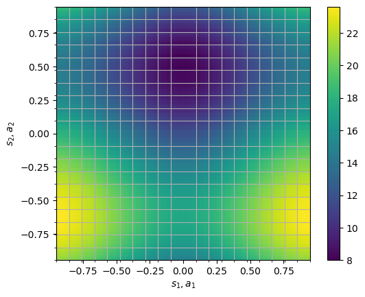
(a) Ground truth value function

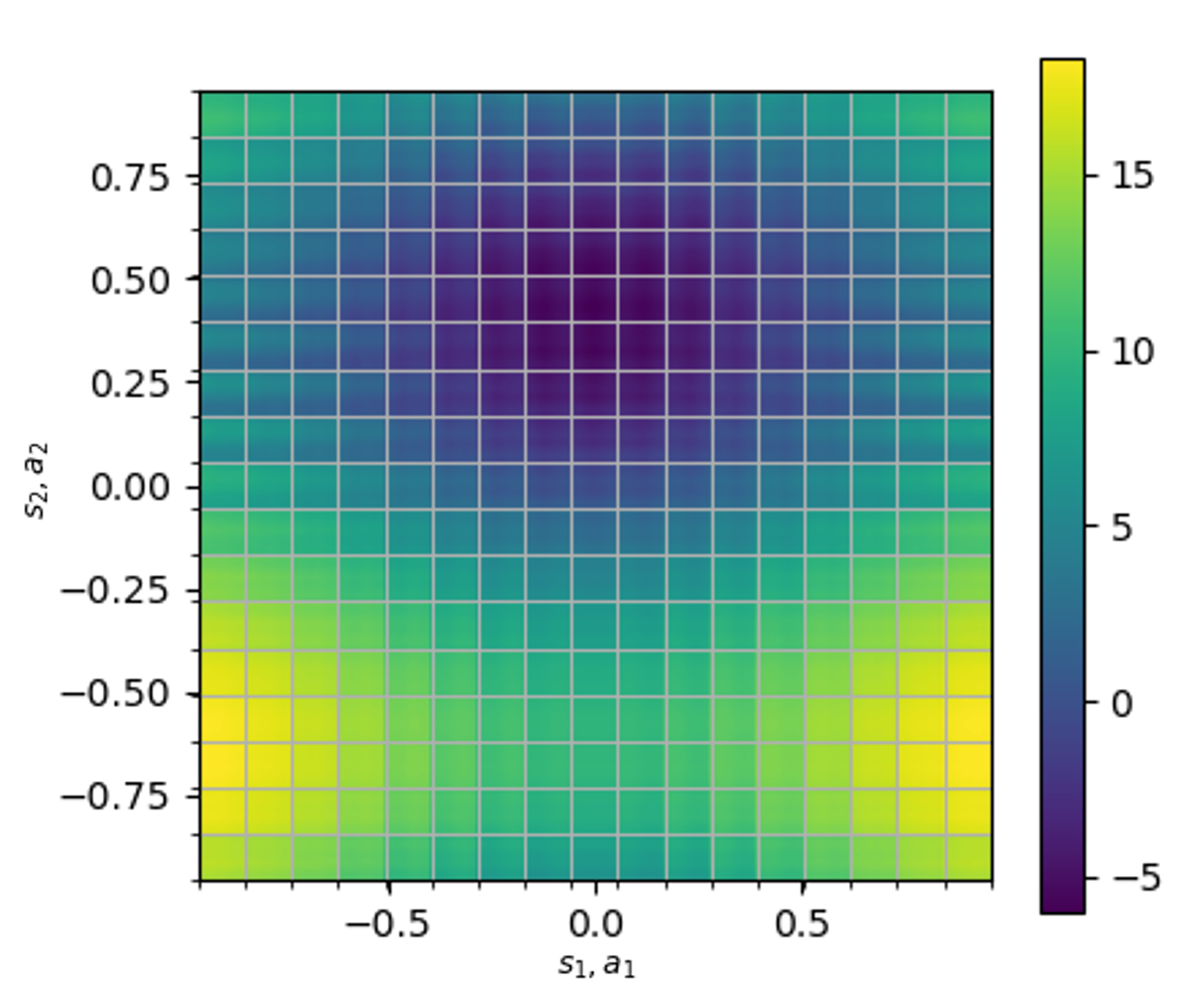
(b) Inferred value function

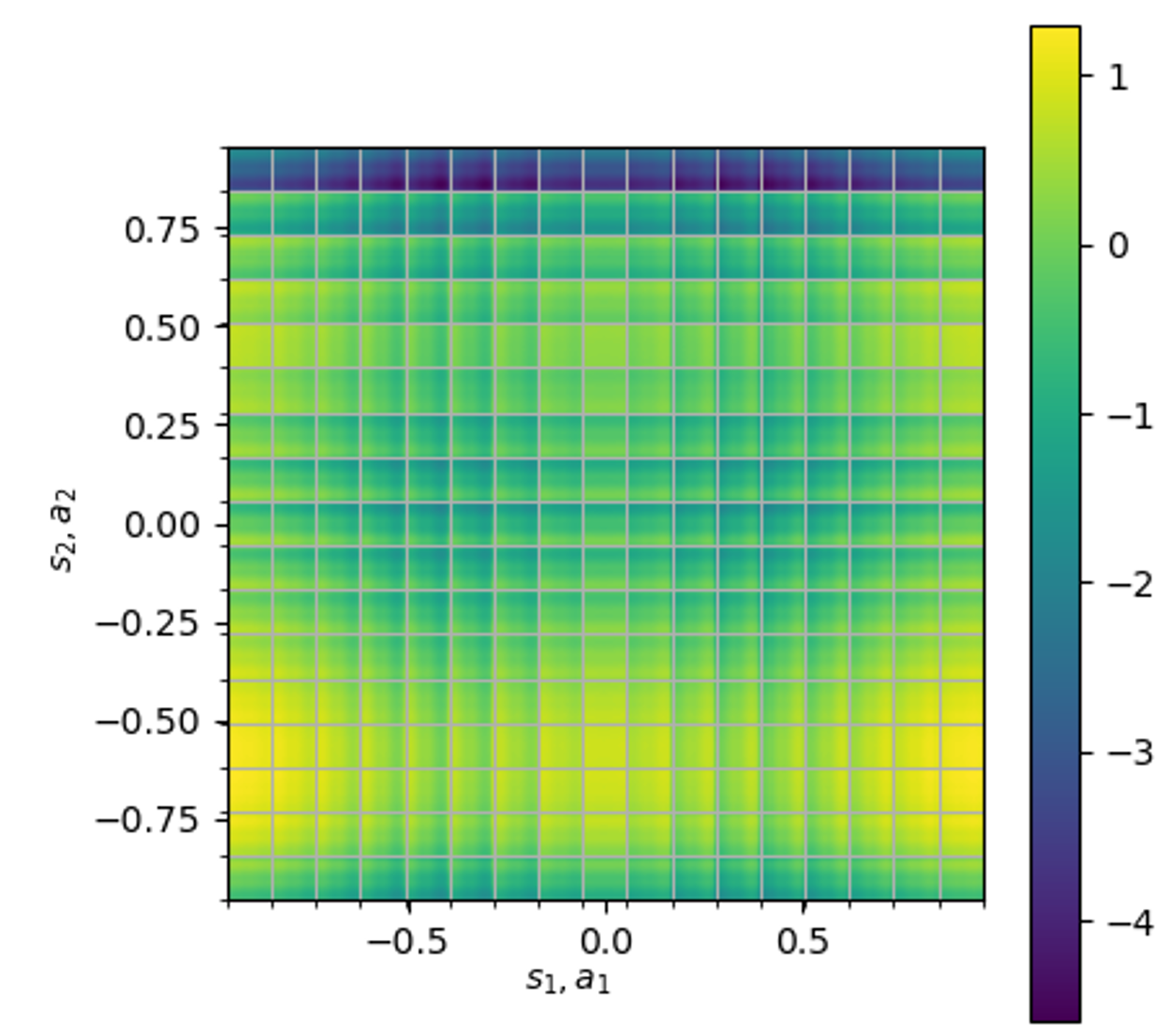
(c) Ground truth reward

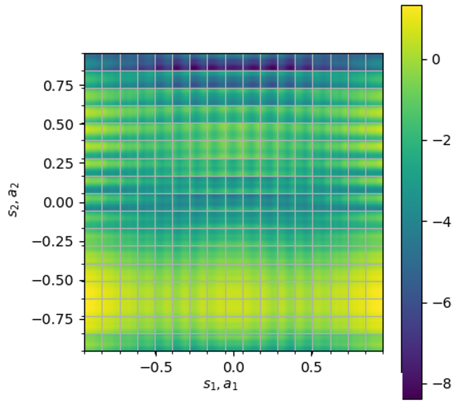
(d) Inferred reward function

Figure 1: Comparison of inferred ground truth value and reward (using highest resolution mesh with $N=17$) with respect to ground truth (plotted with $N=20$)

We also consider the effect of the mesh resolution of the space $\mathcal{S}\times\mathcal{A}$. Previous studies [27, 28] have shown convergence in the inference conducted using VSI method. Here we investigate the convergence in the state-action value function and, consequently, the reward. We consider a box domain with $\Omega=[-1,1]^{4}$ using Cartesian meshes with nodes at $\boldsymbol{x}\in\left\{-1,-1+\frac{2}{N},\cdots,-1+\frac{2i}{N},\cdots,1\right\}^{4}$. We evaluate the error estimated $\psi$ compared to the ground truth state-action value generated using fixed-point iteration (details provided in Appendix B). The results of the convergence analysis are presented in Fig. 2(b) and 2(c) where the error is observed to decrease with finer mesh resolution.

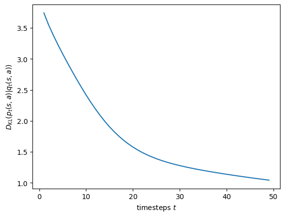
(a)

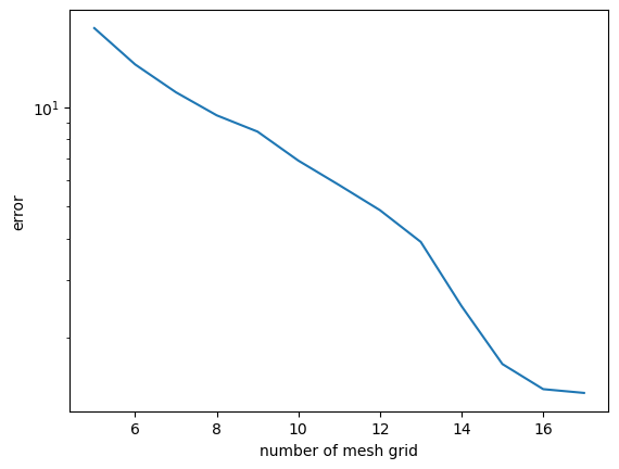
(b)

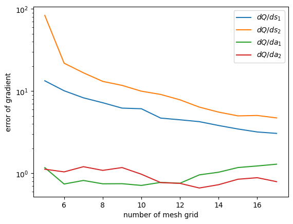
(c)

Figure 2: (a) KL divergence $D_{\mathrm{KL}}(p_{t}|q_{t})$ of the probability distribution between data distribution and simulation probability distribution over time. The errors of the (b) value function and (c) partial derivatives of the value function, estimated as $\frac{1}{|\Omega|}\left(\int_{\Omega}(f(\boldsymbol{x})-f_{\text{GT}}(\boldsymbol{x}))^{2}d\boldsymbol{x}\right)^{1/2}$

4.2 Cancer Cell Metastasis

As a proof-of-concept, we apply our algorithm to a dataset on MDA-MB231 cancer cells in a migration assay Fig. 3(a) [17], which monitors 1332 cells in 361 timesteps. A chemical gradient of the chemo-attractant CXCL12 is applied pointing to the left: the negative horizontal direction. This induces the cells to migrate leftward, on average. We define the x-y velocity $v_{x}$, $v_{y}$ as states, and ERT, Akt as the actions. The data is rescaled to $(-1,1)$ for computation, and we empirically estimate the probability density of cells. Our FP-IRL algorithm applied to this dataset recovers the result that the cell will receive a high reward for moving leftward with a high velocity in agreement with our knowledge about the experimental setup. Interestingly, FP-IRL also uncovers a vertical component to the velocity providing high rewards. These are for the state space, $\mathcal{S}$ corresponding to cell velocities. Additionally, the action space $\mathcal{A}$ in this study corresponds to the expression of kinases ERK and Akt. FP-IRL infers a policy expressing low Akt when moving towards left with high speed to be optimal.

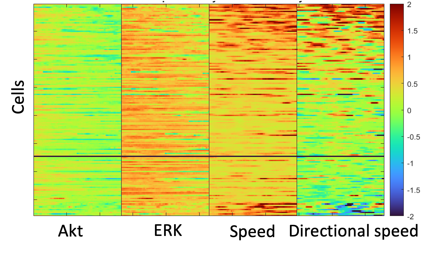
(a)

(b)

Figure 3: (a) Kymograph for the cancer cell migration data: each column shows the different variables measured from that experiment, and each row shows the measurement value over time.(b) Reward and policy inferred from data, the left shows the reward and the right shows the policy

5 Discussion

5.1 Significance

In this work, we have conjectured an isomorphism between the physics of the FP equation of optimal transport and key ideas in MDPs. On this basis, we have proposed a novel physics-based IRL algorithm, and demonstrated it on a problem studying the dynamics of living agents in biology. This approach could initiate a new paradigm of artificial intelligence for physics-based biology, in which we seek to learn the deemed reward gained by cell agents following a policy. With physics-constrained modeling, this allows the application of IRL to problems where the transition is not available and has not been mathematically modeled, or discovered. Computationally, the incorporation of physics results in methods that are less expensive than other generic IRL algorithms: We do not need to solve the forward reinforcement learning problem iteratively (e.g. through a min-max optimization) to evaluate the reward parameters and corresponding policy. Instead, we infer parameters of the physical system, and through our conjecture, obtain the transition, reward and policy. Our physics-based approach also offers an alternative to purely neural network-based methods to uncover the reward function from the system.

5.2 Limitations

One limitation of our approach is that we start from the free energy in Fokker-Planck dynamics; the target dynamics therefore must submit to this description in the continuous limit. Moreover, the stochastic differential equation constrains the state and action space $\mathcal{S}\times\mathcal{A}$ to be $\mathbb{R}^{n}$, where we have described the dynamics using periodic assumptions. Also, we use partial differential equations, limiting the definition of to be continuous. The convergence analysis shows that a finer discretization is required to accurately estimate the potential function. This makes our method less suitable for coarsely binned state-action spaces. The process of identifying an FP equation is not trivial and requires some prior domain knowledge. Finally, our method rests on mean-field physics, and therefore, may not be suitable to study multi-agent systems with interactions in the current setting.

5.3 Future works

There are several directions in which this physics-based framework for IRL can be extended. Possible theoretical extensions include: (1) more expressive diffusive mechanisms like Maxwell-Stephan diffusion that account for collisions between agents and (2) considerations for reflected Brownian motion that describes the evolution of agents in bounded domains. Turning toward additional capabilities for this framework, many physical systems, such as migration mechanics of cells, naturally involve the proliferation and death of these individual agents. Modeling such mechanisms, that involve terminal and source states in MDP, results in reactive mechanisms in FP dynamics. This extension will also be a subject of consequent studies. Furthermore, we observe a correlation between the Markov Potential Game and the concept of potential in free energy functional. Another possible future work is an extension to multi-agent problems and uncovering the inter-agents rewards.

6 Conclusion

We developed a novel physics-based IRL algorithm, FP-IRL, that can uncover both the reward function and transition function even when confronted with limited information about the system under investigation. Our approach leverages the fundamental physics principle of minimization of energy and establishes a conjecture regarding the structural isomorphism between FP and MDP. With the conjecture, we can estimate the reward and transition with low computational expense. We validate the efficacy of our method in a synthetic problem and show that it converges to the true solution as we enhance the resolution of the mesh. Finally, we employ our algorithm to infer the reward structure for dynamics of kinase-dependent migration of cancer cells from experimentally obtained data.

Appendix A Inverse Bellman Operator

In this section, we show the proof for Theorem 3.2.

Note that the proof is similar to the proof of Lemma 3.1 in Appendix 2 of [9], but their inverse Bellman operator is defined as

$$R(\boldsymbol{s},\boldsymbol{a})=(\mathcal{T}Q_{\pi})(\boldsymbol{s},\boldsymbol{a})=Q_{\pi}(\boldsymbol{s},\boldsymbol{a})-\gamma\mathbb{E}_{\begin{subarray}{c}\boldsymbol{s}^{\prime}\sim T(\cdot|\boldsymbol{s},\boldsymbol{a}),\\ \boldsymbol{a}^{\prime}\sim\pi(\cdot|\boldsymbol{s}^{\prime})\end{subarray}}\left[Q_{\pi,\text{soft}}(\boldsymbol{s}^{\prime},\boldsymbol{a}^{\prime})-\log\pi(a^{\prime}|s^{\prime})\right]$$ (24)

where $Q_{\pi,\text{soft}}(\cdot)$ is a so-called soft Bellman equation, but ours is defined as

$$R(\boldsymbol{s},\boldsymbol{a})=(\mathcal{T}Q_{\pi})(\boldsymbol{s},\boldsymbol{a})=Q_{\pi}(\boldsymbol{s},\boldsymbol{a})-\gamma\mathbb{E}_{\begin{subarray}{c}\boldsymbol{s}^{\prime}\sim T(\cdot|\boldsymbol{s},\boldsymbol{a}),\\ \boldsymbol{a}^{\prime}\sim\pi(\cdot|\boldsymbol{s}^{\prime})\end{subarray}}\left[Q_{\pi}(\boldsymbol{s}^{\prime},\boldsymbol{a}^{\prime})\right]$$ (25)

where $Q_{\pi}(\boldsymbol{s},\boldsymbol{a})$ denotes the conventional Bellman expectation function of a policy $\pi(\cdot)$.

Lemma A.1.

The matrix ($I-A$) is nonsingular if the norm of matrix $A$ is less than 1 (i.e. $||A||<1$).

Proof.

Proof by contradiction: Let $I-A$ be singular. Therefore, there exists an $\boldsymbol{x}$ (where $\boldsymbol{x}\neq 0$) such that $(I-A)\boldsymbol{x}=0$. Then, $||\boldsymbol{x}||=||A\boldsymbol{x}||\leq||A||\ ||\boldsymbol{x}||$, and therefore $||A||\geq 1$, which contradicts the ansatz $||A||<1$. Therefore ($I-A$) is nonsingular and invertible. ∎

See 3.2

Proof.

For a fixed transition probability function $T(\boldsymbol{s}^{\prime}|\boldsymbol{s},\boldsymbol{a})$, and a fixed policy probability function $\pi(\boldsymbol{a}|\boldsymbol{s})$ in MDP, the joint transition probability function $T_{\pi}(\boldsymbol{s}^{\prime},\boldsymbol{a}^{\prime}|\boldsymbol{s},\boldsymbol{a})=T(\boldsymbol{s}^{\prime}|\boldsymbol{s},\boldsymbol{a})\pi(\boldsymbol{a}^{\prime}|\boldsymbol{s}^{\prime})$ is fixed as well. The inverse Bellman operator can be denoted in matrix form in the discrete case:

$$\boldsymbol{r}=\boldsymbol{q}-\gamma\boldsymbol{T}_{\pi}\boldsymbol{q}=(\boldsymbol{I}-\gamma\boldsymbol{T}_{\pi})\boldsymbol{q}$$ (26)

where $\boldsymbol{r}\in\mathbb{R}^{n_{s}\cdot n_{a}}$ denotes reward vector, $\boldsymbol{q}\in\mathbb{R}^{n_{s}\cdot n_{a}}$ denotes state-action value vector, $\boldsymbol{T}_{\pi}\in\mathbb{R}^{(n_{s}\cdot n_{a})\times(n_{s}\cdot n_{a})}$ denotes the joint transition matrix, and $n_{s}=|\mathcal{S}|,n_{a}=|\mathcal{A}|$ denotes the number of discretized states and actions, respectively. $(\boldsymbol{I}-\gamma\boldsymbol{T}_{\pi})$ is invertible because $||\gamma\boldsymbol{T}_{\pi}||_{1}<1$ (because $T_{\pi}$ denotes a probability function, i.e. $||\boldsymbol{T}_{\pi}||_{1}=1$, and $\gamma\in[0,1)$), as shown in Lemma A.1 . Therefore, because the inverse Bellman operator is a linear transformation with an invertible square transformation matrix $I-\gamma T$, the inverse Bellman operator $\mathcal{T}$ is a bijection when $T(\cdot),\pi(\cdot)$ are fixed. ∎

Appendix B Variational System Identification

In this section, we present the details for the VSI method in Sec. 3.6

B.1 Finite element interpolation

We consider a d-dimensional hypercube domain, $\Omega=\Pi_{i=\{1,\cdots,d\}}[a_{i},b_{i}]\subset\mathbb{R}^{d}$. A partition of $\Omega$ into elements $\Omega_{e}$ is constructed by first partitioning the line segment $[a_{i},b_{i}]$ along each dimension as $[a_{i},b_{i}]=\cup_{j=1}^{k_{i}}[x_{i}^{j},x_{i}^{j+1}]$ with $x_{i}^{1}=a_{i}$, $x_{i}^{k_{i}}=b_{i}$ and $x_{i}^{j}<x_{i}^{j+1}$. Finally, the $d$-dimensional hypercube element is constructed by taking the tensor product of the grid points as $\Omega_{e=(i_{1},\cdots,i_{d})}=\boldsymbol{\Pi}_{l}[x_{l}^{i_{l}},x_{l}^{i_{l}+1}]$. In the finite element formulation presented here, all function values are known at the grid points and the values within the element are interpolated from the neighbouring grid points as $p(\boldsymbol{x})=\sum_{r=1}^{2^{d}}p_{e(r)}N_{r}(\boldsymbol{x})$. Here $p$ represents the function being interpolated with $\boldsymbol{x}$ inside element, $e$, and $p_{e(r)}$ being the value at the $r^{th}$ neighbour of the $e^{th}$ element. The shape functions, $N_{r}$ are constructed using the tensor product of linear Lagrange interpolations in each dimension. As an example we consider the $4$-dimensional case presented in Sec. 4. We first linearly map coordinates of each element onto a unit hypercube i.e. $\Omega_{e}\rightarrow[0,1]^{d}$, representing the new coordinates with $\boldsymbol{\xi}$. The tensor product basis functions in this case are given as follows:

$$N_{1} =(1-\xi_{1})(1-\xi_{2})(1-\xi_{3})(1-\xi_{4})$$

$$N_{2} =(\xi_{1})(1-\xi_{2})(1-\xi_{3})(1-\xi_{4})$$

$$N_{3} =(1-\xi_{1})(\xi_{2})(1-\xi_{3})(1-\xi_{4})$$

$$N_{4} =(\xi_{1})(\xi_{2})(1-\xi_{3})(1-\xi_{4})$$

$$N_{5} =(1-\xi_{1})(1-\xi_{2})(\xi_{3})(1-\xi_{4})$$

$$N_{6} =(\xi_{1})(1-\xi_{2})(\xi_{3})(1-\xi_{4})$$

$$N_{7} =(1-\xi_{1})(\xi_{2})(\xi_{3})(1-\xi_{4})$$

$$N_{8} =(\xi_{1})(\xi_{2})(\xi_{3})(1-\xi_{4})$$

$$N_{9} =(1-\xi_{1})(1-\xi_{2})(1-\xi_{3})(\xi_{4})$$

$$N_{10} =(\xi_{1})(1-\xi_{2})(1-\xi_{3})(\xi_{4})$$

$$N_{11} =(1-\xi_{1})(\xi_{2})(1-\xi_{3})(\xi_{4})$$

$$N_{12} =(\xi_{1})(\xi_{2})(1-\xi_{3})(\xi_{4})$$

$$N_{13} =(1-\xi_{1})(1-\xi_{2})(\xi_{3})(\xi_{4})$$

$$N_{14} =(\xi_{1})(1-\xi_{2})(\xi_{3})(\xi_{4})$$

$$N_{15} =(1-\xi_{1})(\xi_{2})(\xi_{3})(\xi_{4})$$

$$N_{16} =(\xi_{1})(\xi_{2})(\xi_{3})(\xi_{4})$$

B.2 Residue evaluation

The finite element interpolation results in following form of the residual, which is linear in the PDE parameters, $\beta^{-1},\theta_{(j_{1},\dots,j_{d})}$:

$$\boldsymbol{R}=\boldsymbol{y}-[\boldsymbol{\Xi}_{0},\cdots,\boldsymbol{\Xi}_{(j_{1},\cdots,j_{d})},\cdots]\cdot[\beta^{-1},\cdots,\theta_{(j_{1},\cdots,j_{d})},\cdots]$$

where each entry of the vectors $\boldsymbol{y}$ and $\boldsymbol{\Xi}$ is evaluated for each timestep. The components of $\boldsymbol{y}$, $\boldsymbol{\Xi}$ and $\boldsymbol{\Xi}_{0}$ are:

$$y =\sum_{e}\sum_{r=1}^{2^{d}}\int_{\Omega_{e}}\frac{\partial p_{e(r)}}{\partial t}N_{e(r)}wd\Omega$$

$$\Xi_{0} =\sum_{e}\sum_{r=1}^{2^{d}}\int_{\Omega_{e}}p_{e(r)}\nabla_{x}N_{e(r)}\cdot\nabla_{x}wd\Omega$$

$$\Xi_{(j_{1},\cdots,j_{d})} =\sum_{e}\sum_{r=1}^{2^{d}}\int_{\Omega_{e}}p_{e(r)}N_{e(r)}\nabla_{x}\phi_{(j_{1},\cdots,j_{d})}\cdot\nabla_{x}wd\Omega$$

where $w\in\{\overline{N_{1}},\cdots,\overline{N}_{k1\times\cdots\times k_{d}}\}$ with each each $\overline{N}_{i}$ representing the finite element interpolation of a function that is $1$ on $i^{th}$ node and $0$ on every other node. The integrations are efficiently evaluated using Gauss-Legendre integration method.

B.3 Hermite cubic interpolations for $\psi$

We construct a parameterization for a $d$-dimensional differentiable function as:

$$\phi_{j_{1},\cdots,j_{d}}(\boldsymbol{x})=h_{j_{1}}(x_{1})\times\cdots\times h_{j_{d}}(x_{d})$$

where $h_{k}$ represents the Hermite cubic interpolation along each dimension. This interpolation scheme is based on piecewise cubic polynomials and provides a smooth representation of $\phi_{j_{1},\cdots,j_{d}}(\boldsymbol{x})$. In a 1d Hermite cubic interpolation of a function, for instance $f(x)=\sum_{k}\theta_{k}h_{k}(x)$, the parameters $\theta_{k}$ represent the function values and their derivative values at certain node points. This allows them to be used as a parameterization for differentiable functions.

These functions are described in a piecewise sense such that the each dimension is partitioned into line segments and the interpolant is a cubic polynomial within these segments. Moreover, the value of the function as well as its derivative is well defined at the nodes. This is achieved by considering the following interpolation for any (arbitrary) interval $x\in[x_{0},x_{1}]$ with $x_{0}$ and $x_{1}$ representing the nodes of the segment (element).

$$f(x)=\sum_{i=1}^{4}\theta_{i}h^{e}_{i}(\widehat{x}),\qquad\widehat{x}=(x-x_{0})/(x_{1}-x_{0})$$ (27)

where,

$$h^{e}_{1} =1-3\widehat{x}^{2}+2\widehat{x}^{3}$$

$$h^{e}_{2} =(\widehat{x}-2\widehat{x}^{2}+\widehat{x}^{3})(x_{1}-x_{0})$$

$$h^{e}_{3} =3\widehat{x}^{2}-2\widehat{x}^{3}$$

$$h^{e}_{4} =(-\widehat{x}^{2}+\widehat{x}^{3})(x_{1}-x_{0})$$

Moreover the derivatives of the functions are defined as $f^{\prime}(x)=\sum_{i=1}^{4}\theta_{i}h^{e^{\prime}}_{i}$ where

$$h^{e^{\prime}}_{1} =(-6\widehat{x}+6\widehat{x}^{2})/(x_{1}-x_{0})$$

$$h^{e^{\prime}}_{2} =1-4\widehat{x}+3\widehat{x}^{2}$$

$$h^{e^{\prime}}_{3} =(6\widehat{x}-6\widehat{x}^{2})/(x_{1}-x_{0})$$

$$h^{e^{\prime}}_{4} =-2\widehat{x}+3\widehat{x}^{2}$$

Periodicity in the basis functions is introduced by imposing constraints for function values and the derivatives at the boundaries in the 1-dimensional Hermite cubic interpolation.

Appendix C Synthetic Numerical Experiment Details

This section provides the implementation details of synthetic numerical experiments and the cell migration problem. The code is provided in the supplemental materials folder "fp_irl_main".

C.1 Synthetic Example

We first define the value function $Q(\boldsymbol{s},\boldsymbol{a})$ using the Hermite basis in Sec. B.3 where $a=-1,b=1$. The parameters are provided in the supplemental materials along with the code.

The transition function $T(\boldsymbol{s}^{\prime}|\boldsymbol{s},\boldsymbol{a})$ is acquired by Eq. 6 and Eq. 4:

$$T_{\text{MP}}(\boldsymbol{s}^{\prime},\boldsymbol{a}^{\prime}|\boldsymbol{s},\boldsymbol{a}) =T_{\text{MP}}(\boldsymbol{x}^{\prime}|\boldsymbol{x})=\left(\frac{\beta}{4\pi\Delta t}\right)^{d/2}\exp{\left(\frac{-\beta||\boldsymbol{x}-\boldsymbol{x}^{\prime}+\nabla Q(\boldsymbol{x})\Delta t||^{2}}{4\Delta t}\right)}$$ (6)

$$T(\boldsymbol{s}^{\prime}|\boldsymbol{s},\boldsymbol{a}) =\int_{\mathcal{A}}T_{\text{MP}}(\boldsymbol{s}^{\prime},\boldsymbol{a}^{\prime}|\boldsymbol{s},\boldsymbol{a})\ \mathrm{d}\boldsymbol{a}^{\prime}$$ (4)

The expert policy $\pi^{*}(\boldsymbol{a}|\boldsymbol{s})$ is acquired by Eq. 14:

$$\pi^{*}(\boldsymbol{a}|\boldsymbol{s})=\frac{\exp(\beta Q_{\pi}(\boldsymbol{s},\boldsymbol{a}))}{\int_{\mathcal{A}}\exp(\beta Q_{\pi}(\boldsymbol{s},\boldsymbol{\hat{a}}))\mathrm{d}\boldsymbol{\hat{a}}}$$ (14)

The ground truth reward $R(\boldsymbol{s},\boldsymbol{a})$ (that the agent’s policy maximizes) is acquired by Eq. 18:

$$R(\boldsymbol{s},\boldsymbol{a})=Q_{\pi}(\boldsymbol{s},\boldsymbol{a})-\gamma\mathbb{E}_{\boldsymbol{s}^{\prime},\boldsymbol{a}^{\prime}\sim T(\cdot|\boldsymbol{s},\boldsymbol{a})}\left[Q_{\pi}(\boldsymbol{s}^{\prime},\boldsymbol{a}^{\prime})\right]$$ (18)

Then, the probability distribution over time $\mathcal{D}=\{p_{t}(\boldsymbol{s},\boldsymbol{a})\}_{t}$ is calculated by

$$p_{0}(\boldsymbol{s},\boldsymbol{a}) =\pi(\boldsymbol{a}|\boldsymbol{s})p_{0}(\boldsymbol{s})$$ (28)

$$p_{t}(\boldsymbol{s}^{\prime},\boldsymbol{a}^{\prime}) =\pi(\boldsymbol{a}^{\prime}|\boldsymbol{s}^{\prime})\int_{\mathcal{S}\times\mathcal{A}}{p_{t-1}(\boldsymbol{s},\boldsymbol{a})}T(\boldsymbol{s}^{\prime}|\boldsymbol{s},\boldsymbol{a})\mathrm{d}\boldsymbol{a}\mathrm{d}\boldsymbol{s}$$ (29)

Alternately, we can run the Monte-Carlo simulation for trajectories using transition function $T(\boldsymbol{s}^{\prime}|\boldsymbol{s},\boldsymbol{a})$ and policy $\pi^{*}(\boldsymbol{a}|\boldsymbol{s})$, and then estimate the probability density from trajectories.

After obtaining the probability distribution over time $\mathcal{D}=\{p_{t}(\boldsymbol{s},\boldsymbol{a})\}_{t}$ for $t\in[0,T]$, we input it as data to the variational system identification algorithm Sec. 3.6 and estimate the corresponding potential function $\psi(\cdot)$ from $\mathcal{D}$. Leveraging our 3.1, the estimated value function $\hat{Q}(\cdot)=-\psi(\cdot)$, and therefore the estimated transition $\hat{T}(\cdot)$, policy $\hat{\pi}(\cdot)$, reward $\hat{R}(\cdot)$ can be obtained from the previous steps as well. We then compare the ground truth functions and estimated functions to evaluate the algorithm’s performance.

In the convergence analysis, we vary the mesh resolution from 5 to 17 on each dimension. The complete results are provided in the supplemental materials folder “convergence_analysis".

C.2 Cancer Cell Metastasis

In this problem, we define the $x,y$ velocities $v_{x}$, $v_{y}$ as states, and ERT, Akt values as the actions. Due to the domain difference for each variable, the data is rescaled to $(-1,1)$ for computation, and we empirically estimate the probability density over time of cells. Then, we estimate the potential function $\psi(\cdot)$ using variational system identification.

References

- [1] P. Abbeel and A. Y. Ng. Apprenticeship learning via inverse reinforcement learning. In Proceedings of the Twenty-First International Conference on Machine Learning, ICML ’04, page 1, New York, NY, USA, 2004. Association for Computing Machinery.
- [2] R. Bellman. On the theory of dynamic programming. Proceedings of the national Academy of Sciences, 38(8):716–719, 1952.
- [3] R. Fox, A. Pakman, and N. Tishby. Taming the noise in reinforcement learning via soft updates. In Proceedings of the Thirty-Second Conference on Uncertainty in Artificial Intelligence, UAI’16, page 202–211, Arlington, Virginia, USA, 2016. AUAI Press.
- [4] K. Friston. The free-energy principle: a rough guide to the brain? Trends in cognitive sciences, 13(7):293–301, 2009.
- [5] K. Friston. The free-energy principle: a unified brain theory? Nature reviews neuroscience, 11(2):127–138, 2010.
- [6] K. Friston, J. Daunizeau, and S. Kiebel. Active inference or reinforcement learning. PLoS One, 4(7):e6421, 2009.
- [7] K. Friston, J. Kilner, and L. Harrison. A free energy principle for the brain. Journal of Physiology-Paris, 100(1):70–87, 2006. Theoretical and Computational Neuroscience: Understanding Brain Functions.
- [8] J. Fu, K. Luo, and S. Levine. Learning robust rewards with adverserial inverse reinforcement learning. In 6th International Conference on Learning Representations, ICLR 2018, Vancouver, BC, Canada, April 30 - May 3, 2018, Conference Track Proceedings. OpenReview.net, 2018.
- [9] D. Garg, S. Chakraborty, C. Cundy, J. Song, and S. Ermon. Iq-learn: Inverse soft-q learning for imitation. Advances in Neural Information Processing Systems, 34:4028–4039, 2021.
- [10] I. Goodfellow, J. Pouget-Abadie, M. Mirza, B. Xu, D. Warde-Farley, S. Ozair, A. Courville, and Y. Bengio. Generative adversarial nets. In Z. Ghahramani, M. Welling, C. Cortes, N. Lawrence, and K. Weinberger, editors, Advances in Neural Information Processing Systems, volume 27. Curran Associates, Inc., 2014.
- [11] T. Haarnoja, H. Tang, P. Abbeel, and S. Levine. Reinforcement learning with deep energy-based policies. In D. Precup and Y. W. Teh, editors, Proceedings of the 34th International Conference on Machine Learning, volume 70 of Proceedings of Machine Learning Research, pages 1352–1361. PMLR, 06–11 Aug 2017.
- [12] T. Haarnoja, A. Zhou, P. Abbeel, and S. Levine. Soft actor-critic: Off-policy maximum entropy deep reinforcement learning with a stochastic actor. In J. Dy and A. Krause, editors, Proceedings of the 35th International Conference on Machine Learning, volume 80 of Proceedings of Machine Learning Research, pages 1861–1870. PMLR, 10–15 Jul 2018.
- [13] T. Haarnoja, A. Zhou, K. Hartikainen, G. Tucker, S. Ha, J. Tan, V. Kumar, H. Zhu, A. Gupta, P. Abbeel, et al. Soft actor-critic algorithms and applications. arXiv preprint arXiv:1812.05905, 2018.
- [14] P. Henderson, W.-D. Chang, P.-L. Bacon, D. Meger, J. Pineau, and D. Precup. Optiongan: Learning joint reward-policy options using generative adversarial inverse reinforcement learning. Proceedings of the AAAI Conference on Artificial Intelligence, 32(1), Apr. 2018.
- [15] M. Herman, T. Gindele, J. Wagner, F. Schmitt, and W. Burgard. Inverse reinforcement learning with simultaneous estimation of rewards and dynamics. In A. Gretton and C. C. Robert, editors, Proceedings of the 19th International Conference on Artificial Intelligence and Statistics, volume 51 of Proceedings of Machine Learning Research, pages 102–110, Cadiz, Spain, 09–11 May 2016. PMLR.
- [16] J. Ho and S. Ermon. Generative adversarial imitation learning. In D. Lee, M. Sugiyama, U. Luxburg, I. Guyon, and R. Garnett, editors, Advances in Neural Information Processing Systems, volume 29. Curran Associates, Inc., 2016.
- [17] K. K. Ho, S. Srivastava, P. C. Kinnunen, K. Garikipati, G. D. Luker, and K. E. Luker. Cell-to-cell variability of dynamic cxcl12-cxcr4 signaling and morphological processes in chemotaxis. bioRxiv, 2022.
- [18] T. Hossain, W. Shen, A. D. Antar, S. Prabhudesai, S. Inoue, X. Huan, and N. Banovic. A bayesian approach for quantifying data scarcity when modeling human behavior via inverse reinforcement learning. ACM Trans. Comput.-Hum. Interact., jul 2022. Just Accepted.
- [19] R. Jordan, D. Kinderlehrer, and F. Otto. Free energy and the fokker-planck equation. Physica D: Nonlinear Phenomena, 107(2):265–271, 1997. 16th Annual International Conference of the Center for Nonlinear Studies.
- [20] J. Kalantari, H. Nelson, and N. Chia. The unreasonable effectiveness of inverse reinforcement learning in advancing cancer research. Proceedings of the AAAI Conference on Artificial Intelligence, 34(01):437–445, Apr. 2020.
- [21] A. Y. Ng and S. J. Russell. Algorithms for inverse reinforcement learning. In Proceedings of the Seventeenth International Conference on Machine Learning, ICML ’00, page 663–670, San Francisco, CA, USA, 2000. Morgan Kaufmann Publishers Inc.
- [22] D. Ramachandran and E. Amir. Bayesian inverse reinforcement learning. In Proceedings of the 20th International Joint Conference on Artifical Intelligence, IJCAI’07, page 2586–2591, San Francisco, CA, USA, 2007. Morgan Kaufmann Publishers Inc.
- [23] N. D. Ratliff, J. A. Bagnell, and M. A. Zinkevich. Maximum margin planning. In Proceedings of the 23rd International Conference on Machine Learning, ICML ’06, page 729–736, New York, NY, USA, 2006. Association for Computing Machinery.
- [24] H. Risken and T. Frank. The Fokker-Planck Equation: Methods of Solution and Applications. Springer Series in Synergetics. Springer Berlin Heidelberg, 1996.
- [25] S. Russell. Learning agents for uncertain environments. In Proceedings of the eleventh annual conference on Computational learning theory, pages 101–103, 1998.
- [26] B. Sallans and G. E. Hinton. Reinforcement learning with factored states and actions. The Journal of Machine Learning Research, 5:1063–1088, 2004.
- [27] Z. Wang, X. Huan, and K. Garikipati. Variational system identification of the partial differential equations governing the physics of pattern-formation: Inference under varying fidelity and noise. Computer Methods in Applied Mechanics and Engineering, 356:44–74, 2019.
- [28] Z. Wang, X. Huan, and K. Garikipati. Variational system identification of the partial differential equations governing microstructure evolution in materials: Inference over sparse and spatially unrelated data. Computer Methods in Applied Mechanics and Engineering, 377:113706, 2021.
- [29] L. Yu, J. Song, and S. Ermon. Multi-agent adversarial inverse reinforcement learning. In K. Chaudhuri and R. Salakhutdinov, editors, Proceedings of the 36th International Conference on Machine Learning, volume 97 of Proceedings of Machine Learning Research, pages 7194–7201. PMLR, 09–15 Jun 2019.
- [30] B. D. Ziebart. Modeling Purposeful Adaptive Behavior with the Principle of Maximum Causal Entropy. PhD thesis, Carnegie Mellon University, USA, 2010. AAI3438449.
- [31] B. D. Ziebart, J. A. Bagnell, and A. K. Dey. Modeling interaction via the principle of maximum causal entropy. In Proceedings of the 27th International Conference on International Conference on Machine Learning, ICML’10, page 1255–1262, Madison, WI, USA, 2010. Omnipress.
- [32] B. D. Ziebart, A. Maas, J. A. Bagnell, and A. K. Dey. Maximum entropy inverse reinforcement learning. In Proceedings of the 23rd National Conference on Artificial Intelligence - Volume 3, AAAI’08, page 1433–1438. AAAI Press, 2008.