A semi-parametric estimation method for quantile coherence with an application to bivariate financial time series clustering

Cristian F. Jiménez-Varón^∗, Ying Sun¹, Ta-Hsin Li

Abstract

In multivariate time series analysis, the coherence measures the linear dependency between two-time series at different frequencies. However, real data applications often exhibit nonlinear dependency in the frequency domain. Conventional coherence analysis fails to capture such dependency. The quantile coherence, on the other hand, characterizes nonlinear dependency by defining the coherence at a set of quantile levels based on trigonometric quantile regression. Although quantile coherence is a more powerful tool, its estimation remains challenging due to the high level of noise. This paper introduces a new estimation technique for quantile coherence. The proposed method is semi-parametric, which uses the parametric form of the spectrum of the vector autoregressive (VAR) model as an approximation to the quantile spectral matrix, along with nonparametric smoothing across quantiles. For each fixed quantile level, we obtain the VAR parameters from the quantile periodograms, then, using the Durbin-Levinson algorithm, we calculate the preliminary estimate of quantile coherence using the VAR parameters. Finally, we smooth the preliminary estimate of quantile coherence across quantiles using a nonparametric smoother. Numerical results show that the proposed estimation method outperforms nonparametric methods. We show that quantile coherence-based bivariate time series clustering has advantages over the ordinary VAR coherence. For applications, the identified clusters of financial stocks by quantile coherence with a market benchmark are shown to have an intriguing and more accurate structure of diversified investment portfolios that may be used by investors to make better decisions.

Some key words: Clustering, Financial stocks, Financial time series, Quantile coherence, Quantile spectral analysis, VAR approximation.

Short title: Semi-parametric quantile coherence estimation

1 Introduction

For univariate time series, motivated by the least-squares interpretation of the ordinary periodogram (OP), Li (2012) proposed the quantile periodogram (QPER) based on trigonometric quantile regression. The QPER, like the ordinary periodogram, has an asymptotic exponential distribution where the mean function, known as the quantile spectrum, is a scaled version of the ordinary spectrum of the level-crossing process. In Li (2012) the QPER is shown to be resistant to nonlinear data distortion in the sense that any nonlinear memoryless transformation only affects the scaling constant in the asymptotic distribution in the given quantile. Wise et al. (1977) shows that OP is not resistant to such nonlinear data transformations as the power spectrum is distorted.

The QPER can be extended to multivariate time series, and in particular, the quantile coherence quantifies the nonlinear dependency across time series by defining coherence as a function of quantile levels as well as frequencies. The quantile coherence has an advantage over its ordinary coherence counterpart as its asymptotic distribution relies on the level-crossing cross-spectrum, which, like QPER, is resistant to nonlinear data distortion due to the robustness of quantile regression (Li, 2013). Despite the fact that quantile coherence is a more effective tool, estimating it remains challenging.

In time series analysis, many methods exist to smooth periodograms for univariate time series. For instance, Shumway and Stoffer (2017) presented several nonparametric periodogram smoothing approaches that can be used across frequencies, such as moving-average smoothing. The optimally smoothed spline (OSS) estimator by Wahba (1980) selects the smoothing parameter by minimizing the expected integrated mean square error. Some other common spectral density estimations are based on likelihood. For instance, Capon (1983) used a high-resolution estimation method, known as the maximum-likelihood method (MLM). MLM filters the time series to produce the minimum-variance unbiased estimator of the spectrum. For bivariate time series data, Pawitan and O’sullivan (1994) estimated the spectrum by means of the penalized Whittle likelihood. In terms of parametric estimators, Burg (1975) presented the maximum entropy type of estimators, which in the univariate case results in the autoregressive (AR) of spectral approximation. For quantile periodograms, the quantile spectrum needs to be smoothed across quantile levels as well. Dette et al. (2015) demonstrated that a window smoother of the quantile periodogram may consistently estimate the quantile spectrum. Chen et al. (2021) proposed a semi-parametric estimation of the quantile spectrum by using the approximation capability of the AR model. A nonparametric smoother is proposed to smooth to both quantile levels and AR coefficients in the partial autocorrelation function (PACF) domain.

In this paper, we propose a new quantile coherence estimation technique. This technique is semi-parametric, adopting the parametric version of the (VAR) spectrum as an approximation to the quantile spectral matrix, combined with nonparametric smoothing across quantile levels. First, we derive the quantile autocovariance function (QACF) from the quantile periodograms for each fixed quantile level; second, we compute the VAR parameters from the QACF using the Durbin-Levinson algorithm; the common order of the VAR approximation for all quantile levels is automatically selected by the AIC (Akaike, 1974). Third, we form the initial estimate of quantile coherence using the VAR parameters; and finally, we smooth the initial estimate of quantile coherence along quantile levels for each frequency using a nonparametric smoother. It is reasonable to assume the smoothness of the periodogram along quantile levels does not change much across frequencies. Therefore, we present a cross-validation criterion for selecting the common tuning parameter for all frequencies. The performance of the estimation method is then investigated through simulation studies.

Spectral features including spectral coherence have been used as input for many applications in time series classification and clustering (Euán et al., 2019; Chen et al., 2021). Maadooliat et al. (2018) applied their proposed spectral density estimation methods for brain signal clustering. Euán et al. (2019) developed a coherence-based hierarchical clustering methods with application to brain connectivity. The quantile frequency analysis (QFA) (see, e.g., Li, 2020, 2021) uses a two-dimensional function of the quantile spectral estimate, by varying the quantile level as well as the trigonometric frequency parameter. The QFA method has been used in two ways in classification. The first method treats quantile periodograms as images that can be directly fed into a deep-learning image classifier like convolutional neural networks (CNN). The second method employs to dimension-reduction techniques and feed the resulting features into a general-purpose classifier such as the support vector machine (Hastie et al., 2017). Chen et al. (2021) used the former approach to classify a large number of earthquake waves. Li (2020) used the latter approach to classify real-world ultrasound signals for nondestructive evaluation of the structural integrity of aircraft panels.

Bishnoi and Ravishanar (2018) studied financial time series clustering based on quantile periodogram using stock price data in several sectors. In our application, we consider the pairs of 52 stocks with the S&P $500$ (SPX) financial index as bivariate time series. These bivariate time series are employed to estimate quantile coherence for clustering purposes. We compare quantile coherence-based clusters to the standard time domain approach, which uses the beta coefficient in the Capital Asset Pricing Model (CAPM), and the ordinary coherence equivalent. We show that the quantile coherence provides additional useful information and tends to identify more meaningful clusters.

The rest of the paper is organized as follows. In Section 2, we introduce the quantile spectral matrix and the proposed estimation procedure for quantile coherence. The simulation study is presented in Section 3, and the application to financial time series clustering is described in Section 4. We conclude and discuss the paper in Section 5.

2 Methodology

In this section, we first introduce the quantile spectrum, the quantile periodogram, and the quantile coherence in Section 2.1. In Section 2.2, the multivariate Yule-Walker equations are described. A brief description of the multivariate version of the Durbin-Levinson algorithm is presented in Section 2.3. The VAR representation of the estimated quantile spectral matrix is presented in Section 2.4. Finally in Section 2.5, we present the proposed smoothing procedure for the VAR spectrum.

2.1 Quantile spectrum and quantile coherence

Assume $\{Y_{t,j}\}~{}(j=1,\ldots,k)$ are $k$ stationary random processes. Let $F_{j}(u)$ denote the CDF of $\{Y_{t,j}\}$ which is a continuous function with the derivative $\dot{F_{j}}(u)>0$. Let $\lambda_{j,\alpha}$ denote the $\alpha$ quantile of $\{Y_{t,j}\}$ for $\alpha\in(0,1)$. Finally, Let $\gamma_{\tau,j,j^{\prime}}(\alpha):=\mathbb{P}\{(Y_{t+\tau,j}-\lambda_{j,\alpha})(Y_{t,j^{\prime}}-\lambda_{j^{\prime},\alpha})<0\}$ denote the lag-$\tau$ level-crossing rate of $\{Y_{t,j}\}$ and $\{Y_{t,j^{\prime}}\}$. Then, according to Li (2012, 2013), the quantile cross-spectrum is defined as

$$s_{j,j^{\prime}}(\omega,\alpha)=\eta_{j,\alpha}\eta_{j^{\prime},\alpha}f_{j,j^{\prime}}(\omega,\alpha),$$

where

$$f_{j,j^{\prime}}(\omega,\alpha)=\sum_{\tau=-\infty}^{\infty}\biggl{\{}1-\frac{1}{2\alpha(1-\alpha)}\gamma_{\tau,j,j^{\prime}}(\alpha)\biggl{\}}\exp(i2\pi\omega\tau),~{}i=\sqrt{-1},$$

is called the level-crossing spectrum, and the scaling constants are defined as $\eta_{j,\alpha}:=\sqrt{\alpha(1-\alpha)}/\dot{F}_{j}(\lambda_{j,\alpha})$ and $\eta_{j^{\prime},\alpha}:=\sqrt{\alpha(1-\alpha)}/\dot{F}_{j^{\prime}}(\lambda_{j^{\prime},\alpha})$.

Given the observations $\{Y_{t,j}\}(t=1,\ldots,n)$ and quantile level $\alpha\in(0,1)$, consider the following quantile regression problem

$$\widehat{\bm{\beta}}_{n,j}(\omega,\alpha):=\operatorname*{arg\,min}_{\lambda_{j,\alpha}\in\mathds{R},\bm{\beta_{j}}\in\mathds{R}^{2}}\sum_{t=1}^{n}\rho_{\alpha}(Y_{t,j}-\lambda_{j}-\mathbf{x}_{t}^{\top}(\omega)\bm{\beta}_{j}),$$ (1)

where $\rho_{\alpha}(u):=u(\alpha-\mathds{I}(u<0))$ and $\mathbf{x}_{t}(\omega):=[\cos(2\pi\omega t),\sin(2\pi\omega t)]^{\top}$ for $\omega\in(0,1/2)$.

Let $\widehat{\bm{\beta}}_{n,j}(\omega,{\alpha}):=[\widehat{A}_{n,j}(\omega,\alpha),\widehat{B}_{n,j}(\omega,\alpha)]^{\top}$ denote the quantile regression solution given by Eq. (1), then, the quantile cross-periodogram between $\{Y_{t,j}\}$ and $\{Y_{t,j^{\prime}}\}$ is defined as

$$q_{j,j^{\prime},n}(\omega,\alpha)=nz_{j}(\omega,\alpha)z_{j^{\prime}}^{*}(\omega,\alpha),~{}j,j^{\prime}=1,\dots,k,$$ (2)

where $z_{j}(\omega,\alpha):=\frac{1}{2}\sqrt{n}\{\widehat{A}_{n,j}(\omega,\alpha)-i\widehat{B}_{n,j}(\omega,\alpha)\}$. Notice that when $j=j^{\prime}$ in Eq. (2), it becomes the quantile periodogram of the first kind as in Li (2012). In addition, with $\alpha=0.5$ is the Laplace periodogram by Li (2008) as a special case.

Li (2013) provided the asymptotic properties of the quantile cross-spectrum for the multivariate time series problem. A connection between the quantile periodogram/cross-periodogram and the quantile spectra/cross-spectra was established in Li (2013) (Theorem 11.3), which states that under suitable conditions, the quantile periodogram matrix $\mathbf{Q}_{n}(\omega,\alpha):=[q_{j,j^{\prime};n}(\omega,\alpha)]$ is asymptotically distributed as $\bm{\zeta\zeta}^{\mathsf{H}}$, where $\bm{\zeta}\sim\mathcal{N}_{c}(\mathbf{0},\mathbf{S}(\omega,\alpha))$, with $\mathbf{S}(\omega,\alpha):=[s_{j,j^{\prime}}(\omega,\alpha)]$.

The (squared) quantile coherence between $\{Y_{t,j}\}$ and $\{Y_{t,j^{\prime}}\}$ is defined as

$$c_{j,j^{\prime}}(\omega,\alpha)=\frac{|s_{j,j^{\prime}}(\omega,\alpha)|^{2}}{s_{j,j}(\omega,\alpha)s_{j^{\prime},j^{\prime}}(\omega,\alpha)}.$$ (3)

It takes values between $0$ and $1$

2.2 Yule-Walker equations in multivariate time series

The $k$-variate vector autoregressive (VAR) model is given by (Priestley, 1981)

$$\mathbf{X}_{t}+\mathbf{\Phi}_{1}\mathbf{X}_{t-1}+\ldots+\mathbf{\Phi}_{p}\mathbf{X}_{t-p}=\bm{\epsilon}_{t},$$ (4)

where $\mathbf{X}_{t}$ is a $k$-dimensional vector and $\mathbf{\Phi}_{1},\dots,\mathbf{\Phi}_{p}$ are $k\times k$ matrices, and $\bm{\epsilon}_{t}$ is a multivariate zero mean white noise process. Each of the components of the vector $\bm{\epsilon}_{t}$ is a univariate white noise process, uncorrelated with each other at different time points, but possibly cross-correlated at common time points.

Assuming stationarity on the VAR model, we can obtain the multivariate Yule-Walker equations by multiplying both sides of the Eq. (4) by $\mathbf{X}^{\top}_{t-h}$ and taking expectations. Denote the covariance matrix for $\mathbf{X}_{t}$ of lag $h$ by $\bm{\Gamma}_{X}(h)$, this gives,

$$\bm{\Gamma}_{X}(h)+\mathbf{\Phi}_{1}\bm{\Gamma}_{X}(h-1)+\ldots+\mathbf{\Phi}_{p}\bm{\Gamma}_{X}(h-p)=\mathbf{0},$$

In matrix form, this can be written as

$$-[\bm{\Gamma}(1)\bm{\Gamma}(2)\ldots\bm{\Gamma}(p)]=[\mathbf{\Phi}_{1}\mathbf{\Phi}_{2}\ldots\mathbf{\Phi}_{p}]\widetilde{\mathbf{\Gamma}},$$ (5)

where

$$\widetilde{\bm{\Gamma}}=\begin{bmatrix}\bm{\Gamma}(0)&\bm{\Gamma}(1)&\ldots&\bm{\Gamma}(p-1)\\ \bm{\Gamma}(1)^{\top}&\bm{\Gamma}(0)&\ldots&\bm{\Gamma}(p-2)\\ \vdots&\vdots&\vdots&\vdots\\ \bm{\Gamma}(p-1)^{\top}&\bm{\Gamma}(p-2)^{\top}&\ldots&\bm{\Gamma}(0)\end{bmatrix}$$

The Yule-Walker equations in (5) must be solved for $\mathbf{\Phi}_{r},r=1,\ldots,p$. A brute-force approach requires the inversion of $kp\times kp$ matrices.

2.3 Multivariate Durbin-Levinson Algorithm and the standard partial autocorrelation function

Whittle (1963) proposed the multivariate version of the Durbin-Levinson recursions, which solve the Yule-Walker equations in (5) with a total of $2p$ inversions of $k\times k$ matrices. (see also proposition 11.4.1 Brockwell and Davis, 1991).

Degerine (1990) proposed a way of defining the partial autocorrelation function for multivariate stationary time series through the canonical analysis of the forward and backward innovations. It is proved that there is a one-to-one correspondence between the resulting PACF and the autocovariance function.

Based on Whittle (1963) and the canonical approach defined by Degerine (1990), we employ the following algorithm to compute the VAR parameters recursively. Given a sequences of covariance matrices $\{\bm{\Gamma}(0),\bm{\Gamma}(1),\ldots\bm{\Gamma}(p)\}$,

1. Compute $V_{0}=\widetilde{V_{0}}=\bm{\Gamma}(0)$ and $\Delta_{0}=\bm{\Gamma}(1)$.

2. For $r=1,\ldots,p$, compute the PACF $\mathbf{\Psi}_{r}=\mathbf{V}^{-1/2}_{r-1}\Delta_{r-1}\widetilde{\mathbf{V}}_{r-1}^{-1/2}$.

3. Compute

   $$\mathbf{\Phi}_{r,r} =\mathbf{V}^{1/2}_{r-1}\mathbf{\Psi}_{r}\widetilde{\mathbf{V}}_{r-1}^{2}$$

   $$\widetilde{\mathbf{\Phi}}_{r,r} =\widetilde{\mathbf{V}}_{r-1}^{1/2}\mathbf{\Psi}_{r}^{\top}\mathbf{V}^{1/2}_{r-1}.$$

4. For $p\geq 2$, compute

   $$\mathbf{\Phi}_{r,r^{\prime}} =\mathbf{\Phi}_{r-1,r^{\prime}}-\mathbf{\Phi}_{r,r}\widetilde{\mathbf{\Phi}}_{r-1,r-r^{\prime}},~{}r^{\prime}=1,\ldots r-1$$

   $$\widetilde{\mathbf{\Phi}}_{r,r^{\prime}} =\widetilde{\mathbf{\Phi}}_{r-1,r^{\prime}}-\widetilde{\mathbf{\Phi}}_{r,r}\mathbf{\Phi}_{r-1,r-r^{\prime}},~{}r^{\prime}=1,\ldots r-1.$$

5. Compute

   $$\mathbf{V}_{r} =\mathbf{V}^{1/2}_{r-1}[\mathds{I}-\mathbf{\Psi}_{r}\mathbf{\Psi}^{\top}_{r}]\mathbf{V}^{1/2\top}_{r-1}$$

   $$\widetilde{\mathbf{V}}_{r} =\widetilde{\mathbf{V}}^{1/2}_{r-1}[\mathds{I}-\mathbf{\Psi}^{\top}_{r}\mathbf{\Psi}_{r}]\widetilde{\mathbf{V}}^{1/2\top}_{r-1}$$

   $$\mathbf{\Delta}_{r} =\bm{\Gamma}(r+1)-\mathbf{\Phi}_{r,1}\bm{\Gamma}(r)-\ldots-\mathbf{\Phi}_{r,r}\bm{\Gamma}(1).$$

For the VAR model to be stable, the singular values of the PACF $(\Psi_{r})$ must be less than $1$ in magnitude. Morf et al. (1978) proposed the orthogonalization procedure based on a Gramm-Schmidt process to compute the PACF and the resulting Durbin-Levinson recursion.

2.4 VAR approximation of the quantile spectrum and quantile coherence

2.4.1 The quantile autocovariance function (QACF) and order selection

We use a parametric VAR spectrum of order $p$ to approximate the quantile spectral matrix $\mathbf{S}(\omega,\alpha):=[s_{j,j^{\prime}}(\omega,\alpha)]$ for each $\alpha$. Suppose that $\mathbf{Q}_{n}(\omega_{l},\alpha),l=0,1,\ldots,2n-1$, is the raw extended quantile periodogram matrix obtained from the time series, where $\omega_{l}=l/2n$. Here the Fourier frequencies are computed at the first half and extended by symmetry. The QACF is obtained by the inverse Fourier transform of $\mathbf{Q}(\omega_{l},\alpha)$ as

$$\widehat{\bm{\Gamma}}(h,\alpha)=\sum_{l=0}^{2n-1}e^{i2\pi\omega_{l}h}\mathbf{Q}_{n}(\omega_{l},\alpha),~{}h=0,1,\ldots,n-1.$$ (6)

We use the multivariate Durbin-Levinson algorithm described in Section 2.3 to solve the multivariate Yule-Walker equations in (5) formed by $\widehat{\bm{\Gamma}}(h,\alpha)$ in Eq. (6) for each fixed $\alpha$. This algorithm produces the VAR coefficients $\widehat{\mathbf{\Phi}}(1,\alpha),\ldots,\widehat{\mathbf{\Phi}}(p,\alpha)$ and the residual covariance matrix $\widehat{\mathbf{V}}_{p}(\alpha)$. The VAR spectrum of order $p$ can be expressed as

$$\widehat{\mathbf{S}}(\omega,\alpha)=\widehat{\mathbf{U}}^{-1}(\mathbf{\omega},\alpha)~{}\widehat{\mathbf{V}}_{p}(\alpha)~{}\widehat{\mathbf{U}}^{-\mathsf{H}}(\mathbf{\omega},\alpha),$$ (7)

where,

$$\widehat{\mathbf{U}}(\mathbf{\omega},\alpha)=\mathds{I}-\sum_{r=1}^{p}\widehat{\mathbf{\Phi}}(r,\alpha)e^{-i2\pi r\mathbf{\omega}}.$$

For a given set of quantile levels $\alpha_{m},m=1,\ldots,n_{q}$, we propose to choose the order of the VAR model by minimizing the Akaike information criterion (AIC) (Akaike, 1974), i.e.,

$$\widehat{p}=\operatorname*{arg\,min}_{p\in\{0,1,\ldots,p_{\text{max}}\}}\biggl{\{}\frac{1}{n_{q}}\sum_{m=1}^{n_{q}}n\log|\widehat{\mathbf{V}}_{p}(\alpha_{m})|+2k^{2}p\biggl{\}},$$

where $n$ is the length of the time series, $k$ is the number of time series (Lütkepohl, 2005). Some other order selection criterion includes the Bayesian information criterion (BIC) by Schwarz (1978) and the corrected AIC (AIC_c) by Hurvich and Tsai (1989).

Let the $j,j^{\prime}$-th entry of $\widehat{\mathbf{S}}(\omega,\alpha)$ in (7) be denoted by $\widehat{s}_{j,j^{\prime}}(\omega,\alpha)$. Then, our preliminary parametric estimate of the quantile coherence $\widehat{c}_{j,j^{\prime}}(\omega,\alpha)$ in (3) is defined as

$$\widehat{c}_{j,j^{\prime}}(\omega,\alpha)=\frac{|\widehat{s}_{j,j^{\prime}}(\omega,\alpha)|^{2}}{\widehat{s}_{j,j}(\omega,\alpha)\widehat{s}_{j^{\prime},j^{\prime}}(\omega,\alpha)}.$$ (8)

2.5 Smoothing spline procedure

To enhance the parametric estimator of quantile coherence described in (8), we propose to smooth the estimates across quantile levels by using smoothing splines for each frequency but with a common tuning parameter.

Let the preliminary parametric quantile coherence estimate in (8) be evaluated at $n_{q}$ quantile levels $\{\alpha_{m}\}(m=1,\ldots,n_{q})$. At each frequency $\omega_{l}$, we have a one-dimensional sequence $\{\widehat{c}_{j,j^{\prime}}(\omega_{l},\alpha_{m}):m=1,\ldots,n_{q}\}$ which we would like to smooth by smoothing splines. A simple way of doing so is to apply a standard smoothing spline procedure such as the smooth.spline function in R to each of these sequences independently and let the smoothing parameters be selected by the standard leave-one-out cross-validation technique. There are two potential problems with this simple method. First, using different smoothing parameters for different frequencies may introduce undesirable artifacts of discontinuity across frequencies; moreover, the standard leave-one-out cross-validation criterion is known to be ineffective for dealing with positive correlations (Altman, 1990; Wang, 1998) which we observed in the preliminary coherence estimate across quantile levels. To overcome these difficulties, we propose a smoothing procedure that employs a common $\lambda$ for all frequencies, so that the final quantile coherence estimate can be expressed as

$$\widetilde{c}(\omega_{l},\cdot):=\operatorname*{arg\,min}_{c(\omega_{l},\cdot)}\Biggl{\{}\sum_{m=1}^{n_{q}}[\widehat{c}(\omega_{l},\alpha_{m})-c(\omega_{l},\alpha_{m})]^{2}+\lambda\int_{0}^{1}\left[\frac{\partial^{2}c(\omega_{l},\alpha)}{\partial\alpha^{2}}\right]^{2}d\alpha\Biggl{\}},l=1,\ldots,n_{f}.$$ (9)

To select the common smoothing parameter $\lambda$, we propose a special $\mathcal{K}$-fold cross-validation procedure. At each frequency $\omega_{l}$ the sequence $\{\widehat{c}_{j,j^{\prime}}(\omega_{l},\alpha_{m}):m=1,\ldots,n_{q}\}$ is randomly split into $\mathcal{K}$ (approximately) equal-size groups. At each $\kappa=1,\ldots,\mathcal{K}$, one of the groups is reserved for testing, and the remaining $\mathcal{K}-1$ groups for training. Unlike typical $\mathcal{K}$-fold cross-validation procedure, we use the mean value of the coherence estimates in the training set denoted as $\overline{c}_{\text{pred},\kappa}(\omega_{l})$, to predict the mean value of the coherence estimates in the testing set, denoted as $\overline{c}_{\text{test},\kappa}(\omega_{l})$. The smoothing parameter $\lambda$ is chosen as the minimizer of the following CV criterion

$$\text{CV}(\lambda)=\sum_{\kappa=1}^{\mathcal{K}}\Biggl{\{}\sum_{l=1}^{n_{f}}[\overline{c}_{\text{pred},\kappa}(\omega_{l})-\overline{c}_{\text{test},\kappa}(\omega_{l})]^{2}\Biggl{\}}.$$ (10)

The proposed CV criteria in (10) uses the mean value prediction to deal with the correlation of the sequences across quantile levels. The standard $\mathcal{K}$-fold cross-validation criterion predicts individual values in the test set. Because the residuals are positively correlated, the resulting tuning parameter tends to be very small for all frequencies and the level of smoothing tends to be minimal.

3 Simulation Study

In this section, we present the results of a simulation study where the proposed method is compared with some alternatives in estimating the quantile coherence of simulated time series and the results of clustering bivariate time series based on both the quantile and the ordinary coherence.

3.1 Simulation setup

The models considered in this simulation setting are

1. VAR(2) model: $\mathbf{Z}_{t}=\mathbf{A}_{1}\mathbf{Z}_{t-1}+\mathbf{A}_{2}\mathbf{Z}_{t-2}+\mathbf{W}_{t}$, $\mathbf{W}_{t}\sim\mathbf{\mathcal{N}}(\mathbf{0},\bm{\Sigma})$,

   $$\mathbf{A}_{1}=\begin{bmatrix}1.5&-0.6\\ 0.3&0.2\\ \end{bmatrix}~{}\mathbf{A}_{2}=\begin{bmatrix}-0.5&0.3\\ 0.7&-0.2\\ \end{bmatrix}~{}\bm{\Sigma}=\begin{bmatrix}4&1\\ 1&2\\ \end{bmatrix}$$

2. VARMA(2,1) model: $\mathbf{Z}_{t}=\mathbf{A}_{1}\mathbf{Z}_{t-1}+\mathbf{A}_{2}\mathbf{Z}_{t-2}+\mathbf{W}_{t}-\mathbf{B}_{1}\mathbf{W}_{t-1}$, $\mathbf{W}_{t}\sim\mathbf{\mathcal{N}}(\mathbf{0},\bm{\Sigma})$

   $$\mathbf{A}_{1}=\begin{bmatrix}0.816&-0.623\\ -1.116&1.074\\ \end{bmatrix}~{}\mathbf{A}_{2}=\begin{bmatrix}-0.643&0.592\\ 0.615&-0.133\\ \end{bmatrix}$$

   $$\mathbf{B}_{1}=\begin{bmatrix}0&-1.248\\ -0.801&0\\ \end{bmatrix}~{}\bm{\Sigma}=\begin{bmatrix}4&2\\ 2&5\\ \end{bmatrix}$$

3. Mixture model highly coherent at lower quantiles: the vector time series, $\{\mathbf{Z}_{t}\}=(Z_{t,1},Z_{t,2})^{\top}$ is a nonlinear mixture of three components given by

   $$\xi_{1} :=\mathcal{W}_{1}(U_{t,1})U_{t,2}+(1-\mathcal{W}_{1}(U_{t,1}))U_{t,1}$$

   $$Z_{t,1} :=\mathcal{W}_{2}(\xi_{1})U_{t,3}+(1-\mathcal{W}_{2}(\xi_{1}))\xi_{1},$$

   where $U_{t,1},U_{t,2}$, and $U_{t,3}$ are AR processes of mean zero and variance 1, satisfying

   $$U_{t,1} =0.8U_{t-1,1}+w_{t,1}$$

   $$U_{t,2} =-0.7U_{t-1,2}+w_{t,2}$$

   $$U_{t,3} =0.55U_{t-1,1}-0.81U_{t-2,3}+w_{t,3},$$

   where $w_{t,1}$, $w_{t,2}$, and $w_{t,3}$ are mutually independent Gaussian white noise. The mixing functions $\mathcal{W}_{1}(x)$ and $\mathcal{W}_{2}(x)$ are defined as follows

   $$\mathcal{W}_{1}(x) =\left\{\begin{matrix}0.1&\text{if}&x<-0.8\\ 0.8&\text{if}&x>0.8\\ \end{matrix}\right.$$

   $$\mathcal{W}_{2}(x) =\left\{\begin{matrix}0.5&\text{if}&x<-0.4\\ 0&\text{if}&x>0.4\\ \end{matrix}\right.,$$

   where $\mathcal{W}_{1}(x)$ is linear between $-0.8$ and $0.8$; $\mathcal{W}_{2}(x)$ is linear between $-0.4$ and $0.4$. The first component $U_{t,1}$ has a lowpass spectrum, $U_{t,2}$ has a highpass spectrum, and $U_{t,3}$ has a bandpass spectrum with a bandwidth of an AR(2) model with frequency at $0.20$. The second component $Z_{t,2}$ of the vector time series $\{\mathbf{Z}_{t}\}$, is a delayed copy of $Z_{t,1}$ by 10 time units.

4. Mixture model highly coherent at higher quantiles: the vector time series $\{\mathbf{Z}_{t}\}=(Z_{t,1},Z_{t,2})^{\top}$ is a nonlinear mixture of three components design in a similar way as the previous mixture model. To obtain highly coherence higher quantiles we just use another weighting function $\mathcal{W}_{2}(x)$, which is defined as

   $$\mathcal{W}_{2}(x)=\left\{\begin{matrix}0&\text{if}&x<-0.4\\ 0.5&\text{if}&x>0.4\\ \end{matrix}\right.,$$

   where $\mathcal{W}_{2}(x)$ is linear between $-0.4$ and $0.4$.

In the simulation study, we consider two lengths of $n=500,1000$ for the VAR and VARMA models and $n=512,1024$ for the nonlinear mixtures. For each model and length, we treat the average of 5000 raw quantile periodogram matrix as the quantile spectral matrix from which we get the true quantile coherence. Fig. 1 shows the true quantile coherence ($\mathbf{C}(\omega,\alpha):=\left[c(\omega_{l},\alpha_{m})\right],l=1,\ldots,n_{f},m=1,\ldots,n_{q}$) for the VAR and VARMA models with $n=500$ (top), and for the mixture models with $n=512$ (bottom). We compute the quantile coherence at $93$ quantile levels, $0.04,0.05,\dots,0.96$. We exclude extreme quantiles where the estimators may not have appropriate behaviors.

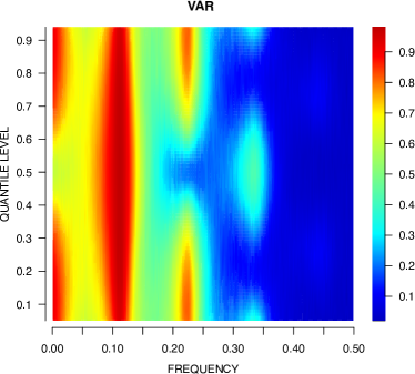
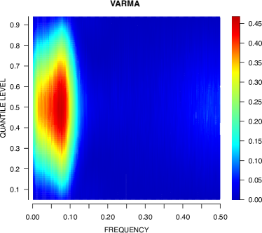
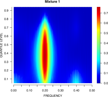
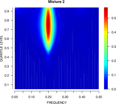
Figure 1: The true quantile coherence of 4 of considered models with $n=500$ for both VAR and VARMA models (top), with $n=512$ for both Mixture 1 and Mixture 2 (bottom).

3.2 Alternative Methods

We compare our proposed estimation method for quantile coherence to two alternative methods. (a) The 1D smoothing spline method: we smooth the raw quantile periodograms using smoothing splines, first across frequencies for each fixed quantile level, and then across quantile levels for each fixed frequency; the coherence is computed based on the resulting smoothed quantile periodogram matrix. (b) The 2D kernel smoothing method: we apply 2D smoothing to the raw quantile periodograms as bivariate functions of frequency and quantile level and compute the quantile coherence from the resulting smoothed quantile periodogram matrix. In addition, we also demonstrate the effectiveness of the smoothing across quantiles by comparing the final estimates in (9) with the preliminary estimates in (8). The parametric method described in Section 2, and second, the semi-parametric estimation that in addition, includes the jointly smoothing procedure presented in Section 2.5.

We use the following root mean squared error (RMSE) between the estimated quantile coherence and the true quantile coherence to measure the performance of an estimator:

$$D_{\text{RMSE}}\{\mathbf{C}(\omega,\alpha),\widetilde{\mathbf{C}}(\omega,\alpha)\}=\sqrt{\frac{1}{n_{f}n_{q}}\sum_{l=1}^{n_{f}}\sum_{m=1}^{n_{q}}[c(\omega_{l},\alpha_{m})-\widetilde{c}(\omega_{l},\alpha_{m})]^{2}}.$$

Table 1 shows the average RMSE from $200$ simulation runs of each case to asses performance where the smoothing parameter by five-fold CV procedures as described in Section 2.5. From Table 1, We can observe that the proposed method consistently outperforms the 1D smoothing splines and 2D kernel smoothing in all cases. Furthermore, with the exception of Mixture 2 ($n=1024$), the RMSE and standard error indicate a decreasing tendency as $n$ increases.

Table 1: The average RMSE of the quantile coherence estimates from 200 simulations. The minimum value in each of the four estimation methods in each row is highlighted in bold. We also include the standard error in parentheses.

Model	n	Semi-Parametric	Parametric	smooth.spline	2D Kernel
VAR (2)	500	0.105 (0.067)	0.115 (0.059)	0.596 (0.105)	0.567 (0.093)
VAR (2)	1000	0.071 (0.049)	0.079 (0.049)	0.415 (0.074)	0.396 (0.058)
VARMA(2,1)	500	0.065 (0.043)	0.072 (0.044)	0.575 (0.360)	0.575 (0.161)
VARMA(2,1)	1000	0.057 (0.040)	0.063 (0.040)	0.579 (0.343)	0.551 (0.130)
Mixture 1	512	0.117 (0.065)	0.121 (0.062)	0.688 (0.233)	0.648 (0.201)
Mixture 1	1024	0.069 (0.037)	0.075 (0.037)	0.645 (0.173)	0.619 (0.157)
Mixture 2	512	0.067 (0.037)	0.069 (0.037)	0.627 (0.353)	0.632 (0.192)
Mixture 2	1024	0.090 (0.046)	0.090 (0.046)	0.627 (0.330)	0.620 (0.163)

3.3 Clustering simulation

In this section, we consider the problem of clustering bivariate $(k=2)$ time series based on the similarities of their quantile coherence. We compare this method with an alternative that employs the ordinary coherence derived from the VAR model of the bivariate time series. Through the simulation study, we would like to show the potential benefit of the quantile coherence for such a problem over the ordinary coherence. To derive the ordinary coherence, we first fit a VAR model to a bivariate time series and then compute the spectral matrix using the parameters from the fitted VAR model. The ordinary coherence is defined by the VAR spectral matrix in a way similar to (7).

The clustering simulation starts by considering the four models described in Section 3.1 as the true clusters. We simulate 100 bivariate time series from each of the four models, then compute their quantile coherence and ordinary coherence. Both the quantile coherence and the ordinary coherence serve as dissimilarity measures for a hierarchical clustering procedure.

For each time series, a feature vector is created by collecting the quantile coherence $c_{1,2}(\omega,\alpha)$ for $l=1,\ldots,n_{f}$ and $m=1,\ldots,n_{q}$. The dissimilarity measure for a pair of time series is defined as the Euclidean distance between the corresponding quantile-coherence-based feature vectors. A similar method is used to define the dissimilarity measure based on the ordinary coherence.

Computing the dissimilarity measure for all pairs allows us to set a pairwise distance matrix, which is used as input for hierarchical clustering. The optimal number of clusters is chosen based on the so-called ”elbow rule” (Yuan and Yang, 2019). This rule uses the total within-cluster sum of squares (WSS) as a function of the number of clusters.

From the right panel of Fig. 2, we can clearly state that the optimal amount of clusters for the quantile coherence equals 4. On the other hand, the left panel of Fig. 2 indicates that the optimal amount of clusters for the ordinary coherence lies between 3 and 4. In a first exploratory exercise, we assumed that the number of clusters acquired by the quantile coherence, 4, was identical to the number of clusters formed from the ordinary coherence in order to evaluate the findings in terms of the allocation of members in each cluster.

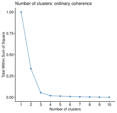
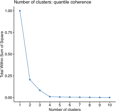
Figure 2: The total within-cluster sum of squares (WSS) as a function of the number of clusters. Based on the ordinary coherence (left), based on the quantile coherence (right).

Although the optimal number of clusters is the same in this case, the allocation results differ substantially. The ordinary coherence assigns the first cluster to the 100 bivariate series acquired by model 1, likewise for the second cluster with model 2. Finally, the remaining 200 bivariate series generated by the mixture models are assigned to the third (79 members) and fourth (121 members) clusters. The third clusters contain only simulated bivariate time series obtained from model 3, while the fourth cluster contains members obtained from both models 3 and 4.

In a second exercise, we chose 3 clusters as the optimal number from the ordinary coherence. The new results show that, as, in the previous example, the first two clusters maintain the assignment of the bivariate series that were generated from models 1 and 2, respectively. The difference now lies in the third cluster, which contains the 200 bivariate series obtained from the mixture models 3 and 4. By using three clusters, the ordinary coherence is not able to differentiate between the two mixture models. In any of the above cases, either when selecting 3 or 4 clusters, ordinary coherence is not able to correctly assign the 3 and 4 mixture models. On the contrary, the quantile coherence allows placing each of the 100 bivariate time series in a specific cluster, allowing a perfect separation of the 4 simulation models.

To show some detail, we simulate the true ordinary coherence for models 3 and 4, which correspond to the mixture models. For each model, we treat the average of 5000 raw VAR periodogram matrix as the VAR spectral matrix from which we get the true ordinary coherence. In both cases, these models present a peak of coherence around frequency $0.20$ as can be seen in Fig. 3. Comparing the results of Fig. 3 with those of Fig. 3, we can see that the difference lies in the fact that model 3 presents a peak of coherence at frequency 0.20, but this is at low and intermediate quantile levels. On the contrary model 4, although it presents the peak at the same frequency, is found at intermediate and high quantile levels. When compared to the ordinary coherence, the quantile coherence offers a more accurate clustering since it contains additional information about quantile levels that can be used to appropriately assign bivariate series, especially with mixture models.

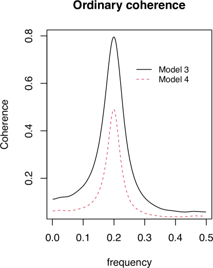
Figure 3: The true ordinary coherence of the 2 mixture models (models 3 and 4), with $n=512$.

4 Financial time series clustering

In this section, we aim to investigate the benefit of clustering the time series of stock prices using their quantile coherence with a benchmark. The objective of this experiment is to see if meaningful clusters of these stocks can be identified based on their co-variability with respect to the benchmark in different quantiles. We chose 52 stocks from the S&P 500 (SPX) somewhat arbitrarily just to evaluate the estimation method for the quantile coherence.

The 52 selected stocks represent different market sectors such as Health Care, Technology, Materials, Consumer Staples, Industrials, Consumer Discretionary, Commodities, Entertainment, Energy, Agricultural Products, Communications Services, Utilities, and Restaurants. Furthermore, the study period is 2010 to 2019, corresponding to a time period free of large oscillations like the ”Great Recession” and the Covid-19 pandemic.

The time series in this experiment comprises the daily close prices of some companies belonging to SPX. The feature vector of each series comprises the quantile coherence between this series and the SPX index evaluated at the Fourier frequencies in $(0,1/2)$ and 93 quantile levels $0.04,\ldots,0.96$. The dissimilarity matrix of these series is defined as the pairwise Euclidean distances of the corresponding quantile-coherence-based feature vector. The resulting dendrogram from the hierarchical clustering procedure is shown in Fig. 4. As discussed in Section 3.3, the optimal number of clusters from the dendrogram is chosen through the so-called ”elbow rule” (Yuan and Yang, 2019). The WSS is represented in Fig. 5, and the optimal number of clusters equals 3.

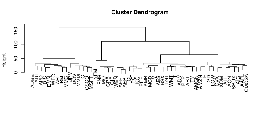
Figure 4: Dendrogram for the hierarchical clustering of 52 stocks in SPX based on the quantile coherence of their daily log returns with the index SPX.

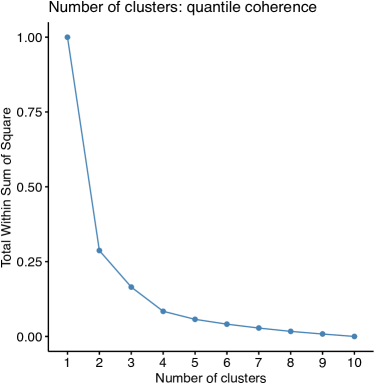
Figure 5: The total within-cluster sum of squares (WSS) as a function of the number of clusters.

In terms of quantile coherence, Cluster 1 stocks are highly coherent at low frequency and at either a very high (greater than 0.75) or very low (less than 0.1) quantile level. It also has considerable quantile coherence in the midrange and high-frequency regions. It is the only one of the three clusters that exhibit this level of activity in terms of quantile coherence in the middle and high-frequency regions. Cluster 2 has a significant level of quantile coherence around low-frequency regions, but it is not as strong as Cluster 1. Furthermore, there is no significant quantile coherence activity in other frequency areas. Finally, Cluster 3 exhibits a significant level of quantile coherence around the lower frequency regions, which is stronger than in Cluster 2 but not as high as in Cluster 1. Cluster 3 contains the largest number of stocks (29). Like Cluster 2, it lacks significant quantile coherence in other frequency ranges; nonetheless, it is significantly higher than in Cluster 2.

The beta coefficient in the Capital Asset Pricing Model (CAPM), a time domain approach, is a standard method of quantifying the systematic risk of equities in the financial industry (Sharpe, 1964; Lintner, 1965; Mossin, 1966). The CAPM methodology distinguishes the stocks that are more sensitive to market movements and those that are less sensitive to such changes. Given that no shocks or other factors caused substantial volatility throughout the period studied, the beta coefficients do not have large values. Stocks with betas above 1 will tend to move with more momentum than the S&P; Stocks with betas less than 1 with less momentum.

The quantile coherence approach creates clusters that are somewhat connected with the beta distribution; but, due to their coherence-quantile connection, the quantile coherence method gives a superior separation among the different stocks. From Table 2, and in terms of beta distribution, we can see two groups of clusters. The first group is cluster 1 which clearly shows the presence mostly of stocks with high betas (higher than 1). The second group is the one formed with clusters 2 and 3 which represent stocks with betas on average less than 1. Clusters 2 and 3 are difficult to distinguish from the beta distribution since their beta-value distributions overlap. Using the quantile coherence, these two clusters are distinguished based on their activity connected with specific quantile areas.

Table 2: Summary statistics for the beta values obtained for each of the four clusters obtained through quantile coherence

Cluster	min	max	mean	sd
Cluster 1	0.8614	1.3352	1.1085	0.1758
Cluster 2	0.3748	0.8624	0.5476	0.1619
Cluster 3	0.4856	1.4966	0.8696	0.2648

To better summarize the information found in each of the three clusters, we compute the centroids of each cluster by averaging the members. In Fig. 6, the highest values of quantile coherence are seen in the low-frequency regions, as well as the lower and upper quantile regions, in all three clusters. Cluster 1 (top left) has the highest coherence. Cluster 3 (Bottom) has a high level of quantile coherence, largely around zero frequency, with some activity in the high-frequency region, although not as much as in Cluster 1. Finally, cluster 2 (top right) only shows activity in terms of quantile coherence around the zero frequency region, with lower values compared to the other two clusters, but only in this region.

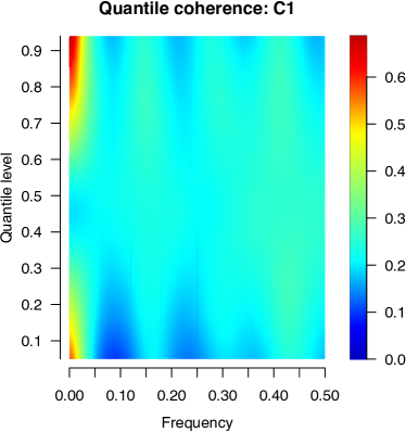
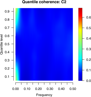
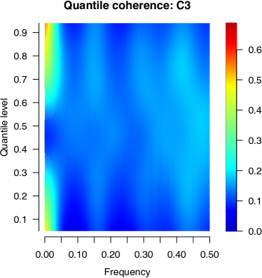
Figure 6: The quantile coherence spectra for the centroids in each of the 3 clusters.

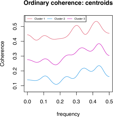
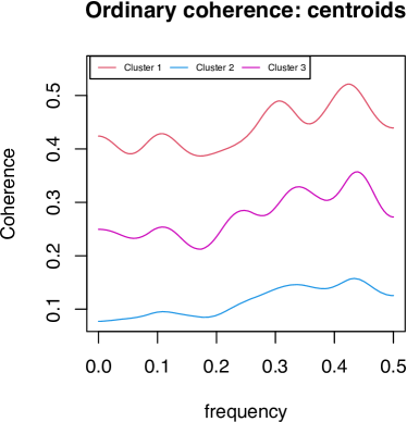
Figure 7: The ordinary coherence spectra for the centroids in each of the 3 clusters. Left. Clusters were obtained from the quantile coherence. Right. Clusters obtained from the ordinary coherence

For comparison, we repeat the hierarchical clustering procedure using the ordinary coherence. The resulting dendrogram is shown in Fig. 8. To select the optimal number of clusters in this case, similar to the quantile coherence case, the elbow plot is in Fig. 9. From Fig. 9 we can see, determining an optimal number of clusters is difficult because no clear turning point can be identified. With the sole purpose of making a fair comparison between the quantile coherence and the ordinary coherence when doing clustering, we use the same number of clusters for the ordinary coherence.

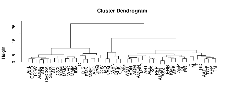
Figure 8: Dendrogram for the hierarchical clustering of 52 stocks in SPX based on the ordinary coherence with the index.

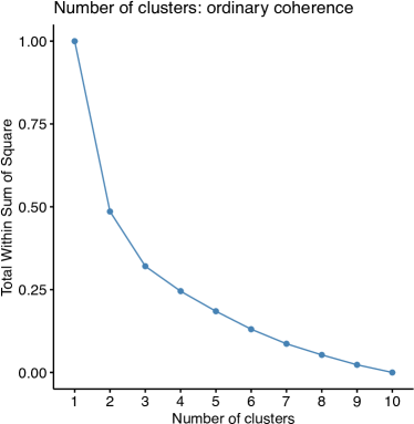
Figure 9: The total within-cluster sum of squares (WSS) as a function of the number of clusters.

We can see from the ordinary coherence that the three clusters exhibit three distinct behaviors (see the centroids for the ordinary coherence in Fig. 7 right panel). Cluster 1 is highly coherent, Cluster 2 is marginally coherent, and Cluster 3 is moderately coherent. In particular, we can see that all of the members in cluster 1 from the quantile coherence are assigned to cluster 1 again in the ordinary coherence; however, this cluster also contains 6 extra members (CVX, CMCSA, SBUX, LOW, ALL, XOM) which were assigned to cluster 3 by the quantile coherence. We can see from the centroid of cluster 3 by the quantile coherence (Fig. 6) these stocks are expected to have substantial coherence around the zero frequency region, similar to cluster 1, and some activity in the middle and higher frequency regions. Furthermore, the level of quantile coherence in the zero-frequency zone is not as high as in the first cluster. Cluster 2 derived from ordinary coherence comprises 5 of the 8 members in cluster 2 derived from quantile coherence. The remaining ones (ENB, AEE, AEP) are assigned to cluster 3 by ordinary coherence. Based on the ordinary coherence ( Fig. 7 right panel and lower plot), cluster 2 contains stocks with low coherence magnitude. These three stocks have moderate quantile coherence and are thus assigned to cluster 3.

Eventually, when we utilized the quantile coherence estimation to acquire the clusters and computed their ordinary coherence, we discovered that these three clusters have a similar partition (left panel of Fig. 7). In terms of ordinary coherence magnitude, the three groups display the same features: high coherence (cluster 1), moderate coherence (cluster 3), and low coherence (cluster 2).

Finally, to better understand the difference in cluster membership, we chose two examples in which the ordinary coherence assigns differently from the quantile coherence: CVX and ENB. For example, CVX belongs to cluster 3 based on quantile coherence but is in cluster 1 based on ordinary coherence; ENB belongs to cluster 2 based on quantile coherence but is in cluster 3 based on ordinary coherence. From the top left panel of Fig. 10, we observe that CVX exhibits a high magnitude of the ordinary coherence, which explains why it is assigned to cluster 1, however, the top right panel shows that this stock does not have a high level of quantile coherence around the zero frequency region, exhibited in the cluster 1 (top left panel of Fig. 6). Similarly, for ENB, from the ordinary coherence (bottom left panel of Fig. 10) we observe a middle range magnitude, however from the quantile coherence estimate (bottom right panel of Fig. 10), the quantile coherence activity is very small and only around the zero frequency region, very similar behavior in cluster 2 (top right panel of Fig. 6 ).

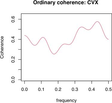
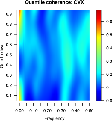
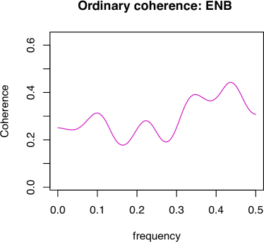
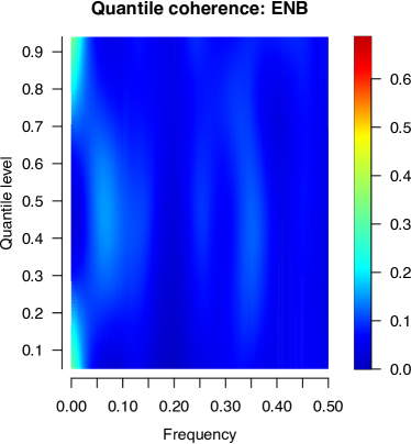
Figure 10: Different classifications between the quantile coherence and the ordinary coherence. Cases of CVX (top panel), and ENB (bottom panel).

Due to the inability of ordinary coherence to relate coherence levels to different quantiles, these results suggest that the quantile coherence is able to provide additional useful information for clustering stocks in accordance with their comovements with financial markets. This is potentially useful to investors in making decisions for the creation of diversified investment portfolios.

5 Discussion

We developed a new semi-parametric method for estimating the quantile coherence derived from trigonometric quantile regression. The proposed method employs the parametric form of the VAR approximation in conjunction with a nonparametric smoothing technique. The parametric VAR spectrum estimates the multivariate quantile spectral matrix at each quantile. The VAR model is obtained by solving the multivariate Yule-Walker equations formed by the quantile autocovariance function which is defined as the inverse Fourier transform of quantile periodograms. The AIC criterion, which balances the goodness of fit and the model complexity is used to determine the VAR order. The resulting preliminary estimate of the quantile coherence is further smoothed across quantiles by smoothing splines where the smoothing parameter is selected jointly across frequencies. For selecting the tuning parameter, a $\mathcal{K}$-fold cross-validation technique is employed to cope with the correlation found in the estimated quantile coherence across quantiles.

Similarly to the quantile periodogram maps previously described in the literature (Li, 2012, 2020), the 2D representation of the quantile coherence provides more information than the ordinary coherence and can be used as images to analyze multivariate time series data.

We also presented the result of an application of quantile coherence to financial time series. In this application, the daily closing prices of 52 stocks are grouped by their behavior against the SPX index as measured by the quantile coherence. The three clusters are distinguished largely by the coherence patterns in the low-frequency region at high and/or low quantiles.

References

- Akaike (1974) Akaike, H. (1974). A new look at the statistical model identification. IEEE Transactions on Automatic Control 19(6), 716–723.
- Altman (1990) Altman, N. S. (1990). Kernel smoothing of data with correlated errors. Journal of the American Statistical Association 85(411), 749–759.