Impact of Beam-Beam Effects on Absolute Luminosity Calibrations at the CERN Large Hadron Collider

Abstract

At the Large Hadron Collider (LHC), absolute luminosity calibrations obtained by the van der Meer () method are affected by the mutual electromagnetic interaction of the two beams. The colliding bunches experience relative orbit shifts, as well as optical distortions akin to the dynamic-$\beta$ effect, that both depend on the transverse beam separation and must therefore be corrected for when deriving the absolute luminosity scale. In the regime, the beam-beam parameter is small enough that the orbit shift can be calculated analytically. The dynamic-$\beta$ corrections to the luminometer calibrations, however, had until the end of Run 2 been estimated in the linear approximation only. In this report, the influence of beam-beam effects on the -based luminosity scale is quantified, together with the associated systematic uncertainties, by means of simulations that fully take into account the non-linearity of the beam-beam force, as well as the resulting non-Gaussian distortions of the transverse beam distributions. Two independent multiparticle simulations, one limited to the weak-strong approximation and one that models strong-strong effects in a self-consistent manner, are found in excellent agreement; both predict a percent-level shift of the absolute $pp$-luminosity values with respect to those assumed until recently in the physics publications of the LHC experiments. These results also provide guidance regarding further studies aimed at reducing the beam–beam-related systematic uncertainty on beam-beam corrections to absolute luminosity calibrations by the van der Meer method.

1 Introduction

The determination of the absolute scale of the luminosity delivered to the ALICE, ATLAS, CMS and LHCb experiments at the LHC relies almost entirely [1] on the van der Meer () method [2, 3]. Luminosity calibrations, which must be performed under specially tailored beam conditions, use beam-separation scans, also known as  scans, to relate the collision rate measured by a given luminometer to the absolute luminosity inferred from directly measured beam parameters. The proportionality between the measured rate and the absolute luminosity is expressed in terms of a “visible” cross-section denoted $\,\sigma_{\mathrm{vis}}$, which is specific to the luminometer and the counting method considered. The precision requirements, which are driven by the LHC physics program, call for -calibration uncertainties in the 1% (0.5%) range at the LHC (HL-LHC).

The beam parameters used to determine the absolute luminosity during  scans are the particle populations and transverse sizes associated with each colliding-bunch pair. During a beam-separation scan, the mutual electromagnetic interaction between two opposing bunches induces separation-dependent orbit shifts, as well as variations in the transverse size and shape of each bunch, thereby distorting the luminosity-scan curves from which the beam-overlap integrals, or equivalently the convolved transverse beam sizes, are extracted. Depending on the beam conditions under which the scans are performed, the magnitude of the resulting calibration bias – if left uncorrected – represents a significant fraction of, or can even exceed, the $\,\sigma_{\mathrm{vis}}$ systematic-uncertainty budget.

The methodology first developed in Refs. [4, 5] to quantify the impact of beam-beam effects on the absolute luminosity scale has been adopted since 2013 by all LHC Collaborations. With as input the beam separation dialed-in at each scan step, plus the measured bunch currents and convolved beam sizes, the orbit shift induced by beam-beam deflections was calculated analytically [6], and the optical distortion associated with the dynamic-$\beta$ effect was evaluated in the linear approximation [4] using the MAD-X package [7]. The two effects impacted the luminosity scale in opposite ways, resulting at the time in a net upwards correction to $\,\sigma_{\mathrm{vis}}$ of 1–1.5% for vdM calibrations at $\sqrt{s}=13$ TeV.

A recent reevaluation of this methodology, using a new beam-beam simulation package specifically developed for -scan studies, revealed that the linear approximation used in the MAD-X simulation results in a significant underestimate of the optical-distortion correction [8]. These findings motivated the studies reported in the present paper, which is organized as follows.

After a brief overview of the -calibration methodology at the LHC and of the impact thereon of beam-beam effects (Sec. 2), the relevant simulation tools are presented in Sec. 3: the MAD-X package used in the original implementation [4, 5]; the B*B package presented in Ref. [8], that models beam-beam dynamics in the transverse plane under the weak-strong approximation; and the long-established COMBI [9] multiparticle code, that is more CPU-intensive but can simulate beam-beam effects in the strong-strong regime with the optional inclusion of longitudinal dynamics. Following a systematic cross-validation of the latter two packages, B*B is used in Sec. 4 to develop an easy-to-use parameterization of beam-beam corrections to  scans in the limit of round, initially Gaussian bunches of equal brightness that collide at a single interaction point (IP) with zero crossing angle. Deviations of the colliding-bunch configuration from this idealized limit: non-Gaussian tails, elliptical transverse bunch profiles, non-zero crossing angle, collisions at multiple IPs, or unequal-brightness beams, are then either accounted for using simulation-based adjustments to the idealized parameterization, or found to be small enough to be treated as a systematic uncertainty. These and other sources of systematic uncertainty, such as tune or $\,\beta^{*}$ settings, that may affect the beam-beam correction in the  regime are consolidated in Sec. 5. An overall summary and a terse outlook are offered in Sec. 6.

2 Luminosity-calibration methodology at the LHC

The -scan formalism [2, 3] that underpins the determination of the absolute luminosity scale at the CERN ISR, RHIC and the LHC is summarized, for the simplest case, in Sec. 2.1 below; generalizations of this formalism can be found in Refs. [8, 10, 11]. At the LHC, because of both instrumental and accelerator-physics reasons [1],  scans are not performed during normal physics operation, but rather under dedicated beam conditions (Sec. 2.2). Their two fundamental ingredients, the transverse beam separation and the measured collision rate, are both affected by the beam-beam interaction (Sec. 2.3), at a level that is significant on the scale of the precision goals outlined in Sec. 1.

2.1 Absolute luminosity scale from measured beam parameters

In terms of colliding-beam parameters, the bunch luminosity ${\mathcal{L}}_{\mathrm{b}}$ is given by

$${\mathcal{L}}_{\mathrm{b}}=f_{\mathrm{r}}\,n_{1}n_{2}\,\int{\hat{\rho}_{1}(x,y)}\,\hat{\rho}_{2}(x,y)\,\mathrm{d}x\,\mathrm{d}y~{},$$ (1)

where the opposing bunches are assumed to collide head-on and with zero crossing angle, $f_{\mathrm{r}}$ is the LHC revolution frequency, $n_{1}n_{2}$ is the bunch-population product and $\hat{\rho}_{1(2)}(x,y)$ is the normalized particle density in the transverse ($x$–$y$) plane of beam 1 (2) at the IP. With the standard assumption that the particle densities can be factorized into independent horizontal and vertical component distributions, $\hat{\rho}(x,y)=\rho_{x}(x)\,\rho_{y}(y)$, Eq. (1) can be rewritten as

$${\mathcal{L}}_{\mathrm{b}}=f_{\mathrm{r}}\,n_{1}n_{2}\,\Omega_{x}(\rho_{x1},\rho_{x2})\,\Omega_{y}(\rho_{y1},\rho_{y2})~{},$$ (2)

where

$$\Omega_{x}(\rho_{x1},\rho_{x2})=\int{\rho_{x1}(x)\,\rho_{x2}(x)\,\mathrm{d}x}$$

is the beam-overlap integral in the $x$ direction (with an analogous definition in the $y$ direction). In the method proposed by van der Meer [2] at the ISR (Fig. 1, top), the overlap integral (for example in the $y$ direction) can be calculated as

$$\Omega_{y}(\rho_{y1},\rho_{y2})=\frac{{R_{y}(0)}}{{\int{R_{y}(\delta_{y})\,\mathrm{d}\delta_{y}}}}~{},$$ (3)

where $R_{y}(\delta_{y})$ is the collision rate, or equivalently the luminosity in arbitrary units, measured during a vertical scan at the time the two beams are separated vertically by the distance $\delta_{y}$. Because the collision rate $R_{y}(\delta_{y})$ is normalized to that at zero separation $R_{y}(0)$, any quantity proportional to the luminosity can be substituted in Eq. (3) in place of $R$.

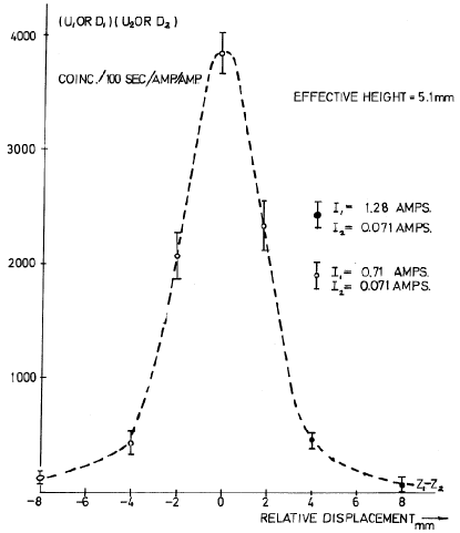
Figure 1: Top: van der Meer method at the CERN ISR. Shown is the monitor rate $R_{y}(\delta_{y})$ as a function of the relative vertical separation $\delta_{y}$ of the two beams (Figure reproduced from Ref. [12], © CERN). Bottom: beam-separation dependence of the visible interaction rate measured at the ATLAS IP during a horizontal  scan in $pp$ collisions at $\sqrt{s}=8$ TeV (LHC fill 3311), before (red circles) and after (purple squares) noise and background subtraction. The subtracted contributions are shown as triangles. The scan curve is fitted to a Gaussian function multiplied by a sixth-order polynomial, plus a constant (Figure reproduced from Ref. [13], © CERN, CC-BY-4.0 license).

Defining the vertical convolved bunch size $\Sigma_{y}$ [1] as

$$\Sigma_{y}=\frac{1}{{\sqrt{2\pi}}}\frac{{\int{R_{y}(\delta_{y})\,\mathrm{d}\delta_{y}}}}{{R_{y}(0)}}~{},$$ (4)

and similarly for $\Sigma_{x}$, the bunch luminosity in Eq. (2) can be rewritten as

$${\mathcal{L}}_{\mathrm{b}}=\frac{f_{\mathrm{r}}n_{1}n_{2}}{{2\pi\Sigma_{x}\Sigma_{y}}}~{},$$ (5)

which allows the absolute bunch luminosity at zero separation to be determined from the revolution frequency $f_{\mathrm{r}}$, the bunch-population product $n_{1}n_{2}$, and the product $\Sigma_{x}\Sigma_{y}$ which is measured directly during a pair of orthogonal scans.

If the transverse density profile of each beam $B$ ($B=1,2$) can be described by a single Gaussian of width $\sigma_{iB}$ ($i=x,y$), the convolved widths are given by

$$\Sigma_{i}=\sqrt{\sigma_{i1}^{2}+\sigma_{i2}^{2}}=\sqrt{\beta^{*}_{i1}\epsilon_{i1}+\beta^{*}_{i2}\epsilon_{i2}}$$ (6)

where $\epsilon_{iB}$ is the geometrical emittance of beam $B$ in plane $i$, and $\beta^{*}_{iB}$ is the corresponding value of the $\beta$ function at the IP. In such a case, the beam-separation dependence of the collision rate is given by

$$R_{i}(\delta_{i})=R_{i}(0)~{}e^{-\frac{\delta_{i}^{2}}{2\Sigma_{i}^{2}}}\,.$$ (7)

The luminosity curve $R_{i}(\delta_{i})$ is also Gaussian, and $\Sigma_{i}$ coincides with the standard deviation of that distribution. It is important to note, however, that the method does not rely on any particular functional form of $R_{i}(\delta_{i})$: the quantities $\Sigma_{x}$ and $\Sigma_{y}$ can be determined for any observed luminosity curve from Eq. (4) and used with Eq. (5) to determine the absolute luminosity at $\delta_{x}=\delta_{y}=0$.

In the more general case where the factorization assumption breaks down, i.e. when the particle densities cannot be factorized into a product of uncorrelated $x$ and $y$ components, Eq. (2) no longer holds, and a single pair of horizontal and vertical scans is no longer sufficient to measure the overlap integral in Eq. (1). One must then generalize the formalism to the two-dimensional case [3], and scan over a grid in the ($\delta_{x},\delta_{y}$) beam-separation space to measure the product of the convolved bunch widths [1, 8]:

$$[\Sigma_{x}\Sigma_{y}]=\frac{1}{{2\pi}}\frac{{\int{R_{x,y}(\delta_{x},\delta_{y})\,\mathrm{d}\delta_{x}\,\mathrm{d}\delta_{y}}}}{{R_{x,y}(0,0)}}~{}.$$ (8)

Here the square brackets highlight the fact that in the presence of non-factorization, the quantity $[\Sigma_{x}\Sigma_{y}]$ can no longer be broken down into a product of two independent quantities. Equation (5), however, remains formally unaffected, as do Eqs. (9)–(10) below.

In terms of luminometer observables, the bunch luminosity can be written as

$$\mathcal{L}_{\mathrm{b}}=\frac{\,\mu_{\mathrm{vis}}\,f_{\mathrm{r}}}{\,\sigma_{\mathrm{vis}}}\,,$$ (9)

where $\,\mu_{\mathrm{vis}}$ is the average number of inelastic collisions per bunch crossing detected by the luminometer considered, and $\,\sigma_{\mathrm{vis}}$ is the associated visible cross-section. Since $\,\mu_{\mathrm{vis}}$ is a directly measurable quantity, the calibration of the absolute luminosity scale amounts to determining the visible cross-section $\,\sigma_{\mathrm{vis}}$. Equating the absolute luminosity computed from beam parameters using Eq. (5) to that measured according to Eq. (9), yields:

$$\,\sigma_{\mathrm{vis}}=\mu_{\mathrm{vis,pk}}\frac{2\pi\,\Sigma_{x}\Sigma_{y}}{n_{1}n_{2}}~{},$$ (10)

where $\mu_{\mathrm{vis,pk}}$ is the visible interaction rate per bunch crossing reported at the peak of the scan curve (Fig. 1, bottom). Equation (10) provides a direct calibration of the visible cross-section $\,\sigma_{\mathrm{vis}}$ in terms of the peak visible interaction rate $\mu_{\mathrm{vis,pk}}$, the product of the convolved bunch widths $\Sigma_{x}\Sigma_{y}$, and the bunch-population product $n_{1}n_{2}$.

In the presence of a significant crossing angle, the formalism becomes more involved [8, 10, 14]. A non-zero crossing angle in either the horizontal or the vertical plane widens the corresponding luminosity-scan curve by the so-called geometrical factor $F$:

$$F=\frac{\sqrt{1+\tan^{2}\,\theta_{c}/2~{}(\sigma_{z1}^{2}+\sigma_{z2}^{2})/(\sigma_{c1}^{2}+\sigma_{c2}^{2})}}{\cos\,\theta_{c}/2}.$$ (11)

Here $\theta_{c}$ is the full crossing angle, $\sigma_{zB}$ ($B=1,2$) are the RMS bunch lengths of beams 1 and 2, and $\sigma_{cB}$ the transverse single-beam sizes in the crossing plane. The peak luminosity is reduced by the same factor. The corresponding increase in the measured value of $\Sigma_{x}$ or $\Sigma_{y}$ is exactly compensated by the decrease in $\mu_{\mathrm{vis,pk}}$, so that Eqs. (4)–(10) remain valid, and no correction for the crossing angle is needed in the determination of $\,\sigma_{\mathrm{vis}}$.

2.2 Beam conditions during van der Meer scans

The strength of the beam-beam interaction is traditionally quantified by the linear beam-beam parameter, defined as [15, 16]:

$$\xi_{x2}=\frac{n_{1}\,r_{0}\,Z_{1}\,Z_{2}\,\beta^{*}_{x2}}{2\pi\,A_{\mathrm{ion},2}\,\gamma_{2}\,\sigma_{x1}(\sigma_{x1}+\sigma_{y1})}$$ (12)

Here $\xi_{x2}$ is the horizontal beam-beam parameter experienced by beam 2 (B2), the “witness beam”; $n_{1}$ is the bunch population of beam 1 (B1), the “source beam”; $r_{0}=e^{2}/4\pi\epsilon_{0}m_{p}c^{2}$ is the classical radius of the proton; $A_{\mathrm{ion},B}$ and $Z_{B}$ ($B=1,2$) are the atomic mass number and charge number of the beam-$B$ particle type (proton or fully stripped ion); $\beta^{*}_{x2}$ is the value of the B2 horizontal $\beta$ function at the IP; $\gamma_{2}$ is the relativistic factor of the B2 particles, and $\sigma_{x1}$ ($\sigma_{y1}$) is the horizontal (vertical) transverse RMS size of B1. Formulas for the other beam and the other plane are obtained by interchanging B1 and B2, and/or $x$ and $y$.

For the most frequent case of $pp$ collisions, Equation (12) takes the more familiar form:

$$\xi_{x2}=\frac{n_{1}\,r_{0}\,\beta^{*}_{x2}}{2\pi\,\gamma_{2}\,\sigma_{x1}(\sigma_{x1}+\sigma_{y1})}\,.$$

In the case of equally populated, equally sized round beams, this expression becomes much simpler:

$$\xi=\frac{nr_{0}\,\beta^{*}}{4\pi\gamma\sigma_{0}^{2}}$$ (13)

where $n$ is the bunch population, and $\sigma_{0}=\sqrt{\epsilon\,\beta^{*}}$ is the nominal RMS beam size at the IP.

In 2018, during high-luminosity physics running in proton-proton ($pp$) mode, the LHC collided up to 2544 bunches with typical initial intensities of $1.1\times 10^{11}$ $p$/bunch, grouped in trains of 36 to 144 bunches with a minimum interbunch spacing of 25 ns. Beams crossed with a half-angle $\theta_{c}/2$ of $\pm 130\,\mu$rad in order to mitigate the impact of the long-range beam-beam interaction at parasitic crossings. At the start of stable beams, the emittance was typically 2 $\mu$m$\cdot$rad [17], the single-bunch luminosity around $7.8\times 10^{30}\,\mathrm{cm}^{-2}\,{\mathrm{s}}^{-1}$ at IP1 and IP5, and the total luminosity close to $1.9\times 10^{34}\,\mathrm{cm}^{-2}\,{\mathrm{s}}^{-1}$ at each of these two IPs. These values correspond to a pile-up parameter $\mu$ of around 55 inelastic $pp$ collisions per bunch crossing, and to a bunch-averaged, head-on beam-beam parameter $\langle\xi\rangle$ of approximately 0.005. The brightness, however, varied significantly along the bunch string, occasionally resulting in $\xi$ values as high as 0.007 for some of the bunches.

In contrast, during $pp$  scans (Table 1), the injected emittance is deliberately blown up and the bunch population significantly lowered, in order to reduce the impact of beam-beam effects as well as minimize the unbunched-beam fraction and the intensity of satellite bunches. The bunches are isolated rather than in trains, and their number is limited to 152 at most, in order to eliminate parasitic crossings and collide with zero crossing angle in the interaction regions where the beam-line layout so permits. The $\beta$ function at the IP is increased such as to bring the pile-up parameter $\mu$ down to around 0.5, i.e. in a regime where luminometers are free of instrumental non-linearities; this carries the additional advantage that it significantly increases the transverse luminous size, allowing a more precise measurement of its beam-separation dependence [1, 13].

Parameter	Typical scans	Reference
	(LHC Run 2)	parameter set
Beam energy $E_{B}$ [TeV]	6.5	3.5
Nominal tune settings $\text{Q}_{x}$/$\text{Q}_{y}$	64.31/59.32	64.31/59.32
Normalized emittance $\epsilon_{N}$ [$\mu$m$\cdot$rad]	2.2 – 3.5	4.00
IP1,5: $\,\beta^{*}$ [m]	19.2	1.50
IP2/8: $\,\beta^{*}$ [m]	19.2 / 24.0	-
IP1,5: $\theta_{c}/2$ [$\mu$rad]	0	0
IP2: $\theta_{c}/2$ [$\mu$rad]	70 – 195 ($y$)	-
IP8: $\theta_{c}/2$ [$\mu$rad]	450 – 550 ($x$)	-
Transverse convolved bunch sizes $\Sigma_{x}\approx\Sigma_{y}$ [$\mu$m]	110 – 160	56.7
Bunch spacing [ns]	$\geq 525$	-
Number of colliding bunches	30 – 124	1
Bunch population $n_{p}$ [$10^{11}$]	0.7 – 1.0	0.85
Linear beam-beam parameter $\xi$ [per IP]	0.0022 – 0.0056	0.0026
Typical bunch luminosity @ IP1, 5 [$\mathrm{cm}^{-2}\,{\mathrm{s}}^{-1}$]	$3-8\times 10^{28}$	$4\times 10^{29}$
Typical total luminosity @ IP1, 5 [$\mathrm{cm}^{-2}\,{\mathrm{s}}^{-1}$]	$2.5-9\times 10^{30}$	$4\times 10^{29}$

Table 1: Beam conditions during  scans at the LHC. Middle column: typical parameters during the 2015-2018 $pp$ scan sessions at $\sqrt{s}=13$ TeV. Right column: reference parameters used for the cross-validation of the beam-beam codes described in Sec. 3; the parameter values are chosen to match those used in the initial, MAD-X based simulations of Ref. [4], which were representative of 2011  scans at IP1 and IP5. In the absence of the beam-beam interaction, the simulated bunches are assumed round in the transverse plane, of equal radius, and strictly Gaussian in all three dimensions.

2.3 Beam–beam-induced biases and their correction

The mutual electromagnetic interaction between colliding bunches shifts their orbits, and therefore modifies their transverse separation at the IP (Sec. 2.3.1); it also distorts their transverse density distributions (Sec. 2.3.2). These two effects depend on the nominal separation $\Delta$ dialed-in at each scan step. Their combination impacts both the normalized integrals ($\Sigma_{x}$, $\Sigma_{y}$) and the peak ($\mu_{\mathrm{vis,pk}}$) of the luminosity-scan curves used in determining the absolute luminosity scale. The strategy for correcting the resulting biases is outlined in Sec. 2.3.3; its detailed implementation is developed in later chapters, in particular in Secs. 4.2.3 and 4.6.5.

2.3.1 Orbit shift

When two positively charged bunches collide with a non-zero impact parameter, they experience a mutually repulsive angular kick equivalent to that of a dipole located at the collision point, the strength of which depends on the beam separation. In the round-beam limit and for $pp$ collisions, the angular kick experienced by a B2 bunch during a horizontal beam-separation scan is given by [18]:

$$\theta_{2x}=\frac{2r_{0}n_{1}}{\gamma_{2}}\frac{\delta_{x}}{\delta}\left[\frac{1-e^{-\delta^{2}/2\Sigma_{R}^{2}}}{\delta}\right],$$ (14)

and similarly for a vertical scan. Here $\delta_{x}$ (resp. $\delta$) is the horizontal (resp. total) beam separation, and $\Sigma_{R}=\Sigma_{x}=\Sigma_{y}$ is the transverse convolved beam size. This formalism has been extended by Bassetti and Erskine [6] and by Ziemann [19] to the case of elliptical beams.

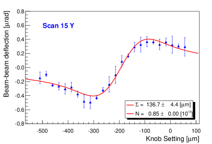
Figure 2: Total beam-beam deflection angle (B1-B2) as a function of the nominal separation $\Delta$ (denoted here by “knob setting”), during a vertical vdM scan at the ATLAS IP in $pp$ collisions at $\sqrt{s}=8$ TeV (LHC fill 3316). For each beam separately, the deflection angle is obtained from the difference between the outgoing- and incoming-beam angles measured by BPMs located in the LHC arcs outside the closed-orbit bump used for the scans. The zero of the horizontal axis is arbitrary, since only relative beam displacements matter. The vertical convolved beam size, denoted here by $\Sigma$, is extracted from a fit to Eq. (14), shown by the red curve, with as input the bunch-averaged population $\mathrm{N}$ (Figure reproduced from Ref. [20], © CERN)

This angular deflection, first observed at the Stanford Linear Collider in $e^{+}e^{-}$ collisions [18], can be measured using beam-position monitors (BPMs) installed both upstream and downstream of the IP, as illustrated in Fig. 2 for the LHC [20].

In a circular collider, the beam-beam angular kick experienced by each beam $B$ ($B=1,2$) in the $i$-plane ($i=x,y$) results in a shift of its position at the IP, given by [21]

$$\delta^{bb}_{iB}=\frac{\beta^{*}_{iB}}{2\,\tan(\pi Q_{i})}~{}\theta_{iB},$$ (15)

where $\,\beta^{*}$ is the value of the $\beta$ function at the IP and $Q_{i}$ is the betatron tune. The actual beam separation at the IP $\delta_{i}$ therefore differs slightly from the nominal separation $\Delta_{i}$:

$$\delta_{i}=\Delta_{i}+\delta^{bb}_{i},$$ (16)

where the beam–beam-induced change in beam separation, hereafter denoted by “orbit shift”, is given by $\delta^{bb}_{i}=\delta^{bb}_{i1}-\delta^{bb}_{i2}$. Since $\delta^{bb}_{iB}$ is, to first order, proportional to the corresponding beam-beam parameter $\xi_{iB}$ (Eqs. (12) and (14)), the orbit shift varies from one bunch to te next. The $\Delta$-dependence of $\delta^{bb}_{i}$ mirrors that displayed in Fig. 2 for the deflection angle, with a peak-to-peak swing of $\pm(1\text{-}2)\,\mu$m under typical -scan conditions, to be compared to typical $\Sigma_{i}$ values in the 110–160 $\mu$m range. The value of $\delta^{bb}_{i}$ changes from scan step to scan step, thereby expanding in a non-linear fashion the beam-separation scale, i.e. the horizontal axis of scan curves such as that illustrated in Fig. 1b. As a result, the overlap integral of Eq. (4) increases by typically 0.7–1.4% per plane, corresponding to a positive correction to $\,\sigma_{\mathrm{vis}}$ in the 1.4–2.8% range.

In practice, the correction for the beam-beam orbit shift is implemented as follows. At each scan step and for each colliding-bunch pair separately, $\delta^{bb}_{i}$ is calculated using the Bassetti-Erskine formula [6], with as input the measured bunch populations ($n_{1},n_{2}$) and uncorrected convolved bunch widths ($\Sigma_{x}$, $\Sigma_{y}$), as well as the beam energy, the $\,\beta^{*}$ setting and the tunes. The separation-dependent collision rate $R_{i}(\delta_{i})$ is then integrated according to Eq. (4) to obtain the beam-beam corrected values $\Sigma^{c,\mathrm{Orb}}_{x}$ and $\Sigma^{c,\mathrm{Orb}}_{y}$, using the beam-beam corrected separation $\delta$ (Eq. (16)) instead of the nominal separation $\Delta$. The agreement of this simple analytical procedure with the predictions of self-consistent multi-particle simulations will be addressed in Sec. 3.5.

2.3.2 Optical distortions

Not only does the electromagnetic field of the B1 bunch deflect the B2 bunch as a whole: it also acts as a non-linear lens that perturbs the trajectory of the individual particles in that bunch, thereby modifying the transverse density distribution of both bunches in a separation-dependent manner.

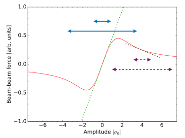
Figure 3: Beam-beam force exerted by the B1 (B2) source bunch as a whole (red curve), as a function of the betatron amplitude of a B2 (B1) test particle, for equally sized round beams. The amplitude is in units of the RMS beam size. The green and brown lines correspond to the linear component of the force at amplitudes of zero and $4\sigma$ respectively, and are akin to the effect of a quadrupole. The short (long) double arrows illustrate the range of transverse kicks experienced by a small (large) amplitude particle for beams either in head-on collision (solid blue lines), or transversely separated by $4\sigma$ (dashed magenta lines).

For small-amplitude particles and beams in head-on collision (Fig. 3, short blue arrows), the force is rather linear and resembles that of a quadrupole (green line), resulting in a tune shift proportional to the beam-beam parameter $\xi$ and in the subsequent dynamic-$\beta$ effect [4]. This “quadrupole strength” is proportional to the derivative of the beam-beam force; it is largest, and repulsive, for small-amplitude particles, changes sign around $1.6\sigma$, and becomes weakly attractive at larger amplitude (dotted brown line).

If for simplicity one assumes that for a given beam separation, all particles are subject to the same quadrupolar-like force (the strength and sign of which depend on the beam separation), then the value of $\,\beta^{*}$ at the scanning IP is modulated by the linear component of the beam-beam force. This results in a modulation of the transverse beam size, and therefore in a beam–separation-dependent modulation of the actual luminosity; however the actual shapes of the transverse density distributions projected on the $x$ and $y$ axes remain unaffected by the quadrupolar-like force. This is the approximation that was adopted in the first implementation of the optical-distortion correction [4, 5], and that will be further discussed in Sec. 3.1.

While for small amplitudes (short arrows) the force remains approximately linear, at amplitudes larger than $1\sigma$ (long arrows) it includes significant non-linear contributions. Large-amplitude particles, therefore, experience a tune shift and a $\beta$-beating that depend both on the particle amplitude (short vs. long arrows) [22], and on the beam separation (blue vs. magenta arrows). The resulting optical distortions include not only a change in optical magnification as in Ref. [4], but also distortions of the shape of the transverse density distributions. Describing their beam-separation dependence requires numerical simulations, that are detailed in Sec. 3.

In practice, the correction for optical distortions is implemented as follows. Separately for each scan step in a horizontal and vertical -scan pair, the luminosity-bias factor $[\mathcal{L}/\mathcal{L}^{0}]_{\mathrm{Opt}}$ associated with beam–beam-induced optical distortions is extracted, as a function of the nominal separation $\Delta_{i}$, from one of the multiparticle simulations described in Sec. 3. Here $\mathcal{L}$ refers to the luminosity that would be measured in the presence of beam-beam optical-distortion effects, and $\mathcal{L}^{0}$ is the corresponding luminosity if beam-beam effects were turned off altogether, all other conditions remaining unchanged. The quantity $\mathcal{L}^{0}$ is dubbed the nominal luminosity; it is akin to “Monte Carlo truth”, and is accessible in the simulation only. The beam-beam corrected collision rate $R^{c}_{i}(\delta_{i})$ is then computed by dividing the measured collision rate by this simulation-based luminosity-bias factor:

$$R^{c}_{i}(\delta_{i})=\frac{R_{i}(\Delta_{i})}{[\mathcal{L}(\Delta_{i})/\mathcal{L}^{0}(\Delta_{i})]_{\mathrm{Opt}}}$$ (17)

and used instead of $R_{i}(\delta_{i})$ in computing the beam-beam corrected convolved bunch sizes $\Sigma^{c,\mathrm{Opt}}_{x}$ and $\Sigma^{c,\mathrm{Opt}}_{y}$ (Eq. (4)), the peak rate $\,\mu^{c}=\mu_{\mathrm{vis,pk}}\,R^{c}_{i}(0)/R_{i}(0)$, and from these quantities the visible cross-section $\,\sigma^{c\mathrm{,Opt}}_{\mathrm{vis}}$ (Eq. (10)).

2.3.3 Beam-beam correction strategy

Conceptually, the principle of the beam-beam correction to  calibrations is to determine the visible cross-section $\,\sigma^{c}_{\mathrm{vis}}$ from the convolved bunch sizes and peak collision rates corrected both for the orbit shift (Sec. 2.3.1) and for optical distortions (Sec. 2.3.2), i.e. corrected to the values ($\Sigma^{c}_{x}$, $\Sigma^{c}_{y}$, $\,\mu^{c}$) that these observables would take if the beam-beam interaction could be turned off during the scan. The quantity $\,\sigma^{c}_{\mathrm{vis}}$ is then the proportionality constant that translates a measured visible interaction rate $\,\mu_{\mathrm{vis}}$ into the corresponding bunch luminosity $\mathcal{L}_{\mathrm{b}}$. It is important to note that even though the actual luminosity is always modified by the beam-beam interaction, including during head-on collisions typical of routine physics running, beam-beam corrections are only needed during scans, basically because the beam-separation dependence of the beam-beam effects distorts the -scan curves. Once $\,\sigma^{c}_{\mathrm{vis}}$ has been determined as specified above, it can always be used to translate the measured collision rate into luminosity units, irrespective of the extent to which this collision rate has been enhanced by the beam-beam interaction.

In practice, orbit-shift and optical-distortion corrections must be applied on a bunch-by-bunch basis, with as inputs the measured bunch populations ($n_{1},n_{2}$) and uncorrected convolved bunch widths ($\Sigma_{x}$, $\Sigma_{y}$), as well as the beam energy, the $\,\beta^{*}$ setting and the tunes. In many cases, these corrections can be extracted from a one-time parameterization of the simulation results in terms of the bunch-specific beam-beam parameter value and of the nominal tunes $\text{Q}_{x}$, $\text{Q}_{y}$. This procedure avoids the repeated use of CPU-intensive, time-consuming multiparticle simulations; it is detailed in Sec. 4.

3 Beam-beam simulation codes

Beam-beam corrections to  calibrations were originally based on MAD-X (Sec. 3.1). Since then, only the zero-separation case has proven amenable to analytical treatment (Sec. 3.2). Beam–separation-dependent effects have been investigated using two independent multiparticle codes dubbed B*B (Sec. 3.3) and COMBI (Sec. 3.4), that have been extensively cross-validated (Sec. 3.5).

3.1 Linear approximation with MAD-X

Since the linear part of the beam-beam force is similar to a quadrupolar field (Fig. 3), one expects the beam-beam interaction to contribute additional focusing or defocusing, thereby shifting the tunes and affecting the optical functions all around the ring, including at the IP itself: this is known as the “dynamic-$\beta$” effect. In the specialized case of equally sized round beams colliding head-on at a single location, the resulting change in the $\beta$ function at the IP is given by [4]:

$$\frac{\,\beta^{*}}{\beta^{*}_{0}}=\frac{1}{\sqrt{1-4\pi\xi\cot(2\pi\mathrm{Q})-4\pi^{2}\xi^{2}}}$$ (18)

where $\beta^{*}_{0}$ is the value of the unperturbed $\beta$ function at the IP, $\,\beta^{*}$ its value in the presence of the beam-beam interaction and Q the tune. The beam-beam parameter $\xi$ is proportional to the derivative of the beam-beam force. Equation (18) implies that the beam-beam induced change in the IP $\beta$ function, and therefore in the IP beam-size squared and in the luminosity, depends only on $\xi$ and on Q. In addition, this dynamic-$\beta$ effect is, to first order, proportional to $\xi$. This is the physical motivation underlying the parameterized-correction approach developed in Sec. 4.

In Ref. [4], the general-purpose optics code MAD-X [7] was used to model the dynamic-$\beta$ effect during simulated  scans. In this software package, beam-beam elements can be inserted at one or several IPs, and their impact on the tunes and on the single-particle optical functions computed as a function of the beam separation $\Delta$. The procedure effectively assumes that for a given beam separation, all particles in the bunch experience the same beam-beam kick, equal to that applied to a zero-amplitude particle for that particular value of $\Delta$. Unperturbed bunches are implicitly supposed to be strictly Gaussian, and to remain so in the presence of the beam-beam interaction: only the change in optical magnification between the LHC arcs and the IP is accounted for in this method.

This study was carried out for the reference parameter set listed in Table 1. The corrections were then adapted to the beam conditions of different  sessions, using the assumption that $\Delta\beta/\beta^{*}_{0}=\,\beta^{*}/\beta^{*}_{0}-1$ scales linearly with the value of $\xi$ inferred from the beam parameters measured during each scan. The simulated beam-separation dependence of the transverse beam size squared, i.e. the value of $(\mathcal{L}/\mathcal{L}^{0})^{-1}$, is illustrated in Fig. 4. Under head-on conditions ($\Delta=0$), the intrinsically defocusing beam-beam force results in a $\sim 0.7$% reduction of the beam size squared at the IP, i.e. to an increase of the luminosity $\mathcal{L}$. This apparent contradiction results from the numerical value of the fractional tunes the LHC optics was designed for (Eq. (18)). As $\Delta$ increases, the tune shift and the dynamic-$\beta$ effect weaken, change sign (in the scanning plane only) around $\Delta/\sigma^{0}\sim 1.6$, then peak and finally vanish asymptotically at very large separation. The change in optical magnification at $\Delta=0$ is slightly different in the $x$ and $y$ planes, because the corresponding fractional tunes $\text{q}_{x}$ and $\text{q}_{y}$ differ by design; the difference in beam-separation dependence also reflects the fact that the vertical kick never changes sign during a horizontal scan, while the horizontal kick does.

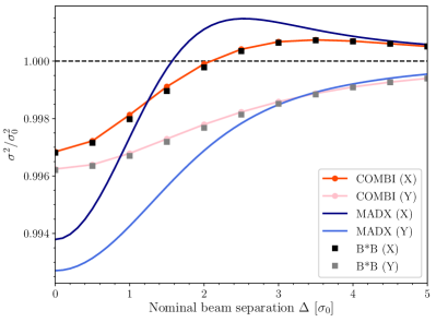
Figure 4: Beam-separation dependence of the transverse RMS beam sizes during a simulated horizontal  scan. The unperturbed beams are assumed to be round and perfectly Gaussian; their parameters are listed in the right column of Table 1. The vertical axis is the ratio squared of the actual beam size $\sigma$ to its unperturbed value $\sigma_{0}$; the horizontal axis is the nominal beam separation in units of $\sigma_{0}$. The MAD-X calculation of the single-particle dynamic-$\beta$ effect (blue curves) is compared to the results of the B*B (square markers) and COMBI (red curves) multiparticle codes. The dark- and light-colored curves and markers illustrate the evolution, during the horizontal scan, of the horizontal and the vertical beam size respectively.

Historically, the optical-distortion correction to $\,\sigma_{\mathrm{vis}}$ predicted by MAD-X under typical Run-1 and Run-2  conditions lay in the 0.2–0.4% range, much smaller than that associated with the orbit effect. For a long time, therefore, it was considered small enough that even if imperfect, it remained sufficiently accurate in view of the systematic uncertainty assigned at the time to the overall beam-beam correction, as documented e.g. in Refs. [5, 13].

In hindsight, however, the limitations of applying the MAD-X approach to beam-beam corrections may not have been fully appreciated. Since at zero beam separation, the slope of the beam-beam force is steepest for zero-amplitude particles (Fig. 3, green line), and since in MAD-X all particles in the witness bunch are assumed to experience the same linearized force, the dynamic-$\beta$ effect predicted by MAD-X at $\Delta=0$ is likely to be an overestimate; this is confirmed analytically below. The situation is reversed at large beam separation: here the derivative of the force is larger at large amplitude (green line) than at small amplitude (brown line), suggesting that MAD-X underestimates the optical distortions at large beam separation. This conjecture, however, can only be confirmed using multiparticle simulations.

3.2 Analytical estimate of optical distortions at zero beam separation

The particle phase space at any location $s$ along a storage ring is described by an ellipse, the shape of which depends on $s$ in a manner described by the well known Courant-Snyder parameters $\alpha$, $\beta$ and $\gamma$ [16]:

$$J_{u}=\frac{1}{2}(\gamma_{u}u^{2}+2\alpha_{u}up_{u}+\beta_{u}p_{u}^{2})\ .$$

Here $u=x,y$ is the deviation of the single-particle orbit from the reference trajectory, $p_{u}=du/ds$, and $J_{u}$ is the action variable that represents the invariant of the motion for each single particle when the reference energy is not changing. The particle position in transverse phase space is fully described by the action $J_{u}$ and by the corresponding phase variable $\phi_{u}$ defined as:

$$\tan{\phi_{u}}=-\beta_{u}\frac{p_{u}}{u}-\alpha_{u}\ .$$ (19)

In addition to distorting the closed orbit, the beam-beam interaction acts as a non-linear electromagnetic lens that includes a quadrupolar term; the latter affects the optical functions $\beta$ and the betatron tunes of the individual particles [22, 23]. During a  scan and for each colliding bunch, the quadrupolar component of the electromagnetic field of the opposing bunch changes as a function of the relative transverse separations $\delta_{i}$ ($i=x,y$) between the beams centroids, and of the single-particle transverse actions $J_{x}$ and $J_{y}$  [23, 24]. This results in a shift in the betatron tune, the so-called detuning with amplitude, given by [25]:

$$\Delta\text{Q}_{x}(J_{x},J_{y})=-\xi_{x}\int_{0}^{\infty}\frac{1}{(1+t)^{2}}~{}e^{-\frac{J_{x}+J_{y}}{2\epsilon(1+t)}}\times$$

$$\left[I_{0}\left(\frac{J_{x}}{2\epsilon(1+t)}\right)-I_{1}\left(\frac{J_{x}}{2\epsilon(1+t)}\right)\right]\times$$

$$I_{0}\left(\frac{J_{y}}{2\epsilon(1+t)}\right)\mathrm{d}t$$

Here $\xi_{x}$ is the beam-beam parameter, $I_{0}$ and $I_{1}$ are modified Bessel functions of the first kind, $\epsilon$ is the emittance (assumed equal in $x$ and $y$), and $t$ is a bound variable. This integral can only be solved when one action is zero, obtaining (for $J_{y}=0$):

$$\Delta\text{Q}_{x}(J_{x}) = -\xi_{x}\frac{2\epsilon}{J_{x}}\left[1-I_{0}\left(\frac{J_{x}}{2\epsilon}\right)\,e^{-\frac{J_{x}}{2\epsilon}}\right]\,$$ (20)

$$\Delta\text{Q}_{y}(J_{x}) = -\xi_{x}\left[I_{0}\left(\frac{J_{x}}{2\epsilon}\right)+I_{1}\left(\frac{J_{x}}{2\epsilon}\right)\right]\,e^{-\frac{J_{x}}{2\epsilon}}\,.$$

For a zero-amplitude particle ($J_{x}=J_{y}=0$) and beams in head-on collision ($\delta_{x}=\delta_{y}=0$), the change in tune is equal to the beam-beam parameter $\xi_{x}$.

Head-on beam-beam $\beta$-beating can be derived from the tune shift in Eq. (20) as:

$$\frac{\Delta\beta_{x}}{\beta_{x}}(J_{x},J_{y}) = -\frac{\Delta\text{Q}_{x}(J_{x},J_{y})}{\xi_{x}}\cdot\frac{\Delta\beta_{0}}{\beta_{x}}$$ (21)

where

$$\frac{\Delta\beta_{0}}{\beta_{x}}=\frac{\Delta\beta_{x}}{\beta_{x}}(0,0)$$

is the linear $\beta$-beating or, equivalently, the $\beta$-beating at $J_{x}=J_{y}=0$.

In the zero-separation case, the $\beta$-beating averaged over the particle distribution (assumed Gaussian) can be calculated as:

$$\overline{\frac{\Delta\beta}{\beta_{x}}} = \int_{0}^{\infty}dJ_{x}\int_{0}^{\infty}dJ_{y}\frac{\Delta\beta_{x}}{\beta_{x}}(J_{x},J_{y})e^{-J_{x}-J_{y}}$$

$$\approx 0.633~{}\frac{\Delta\beta_{0}}{\beta_{x}}\,.$$

For bunches colliding with zero transverse separation, therefore, the particle-action distribution is modified such that the average beam-beam beating is reduced to about $63\%$ of the single-particle estimate computed in Ref. [4]. The corresponding impact on the head-on luminosity can be derived analytically, as follows.

The RMS single-beam size $\sigma_{x}=\sqrt{\beta_{x}\,\epsilon}$, including the action-dependent, beam–beam-induced $\beta$-beating given by Eq. (21), is computed using the following relation:

$$x^{2} = 2\beta_{x}J_{x}\left(1+\frac{\Delta\beta_{x}}{\beta_{x}}\right)\cos^{2}\phi_{x}=$$

$$= \beta_{x}J_{x}\left(1+\frac{\Delta\beta_{x}}{\beta_{x}}\right)(1+\cos 2\phi_{x})\,.$$

Assuming Gaussian particle-density distributions, this yields

$$\sigma_{x}^{2}=\int_{0}^{\infty}dJ_{x}\int_{0}^{\infty}dJ_{y}\int_{0}^{2\pi}\frac{d\phi}{2\pi}\ x^{2}e^{-J_{x}-J_{y}}$$

$$=\beta_{x}\left(1+\int_{0}^{\infty}dJ_{x}\int_{0}^{\infty}dJ_{y}e^{-J_{x}-J_{y}}J_{x}\frac{\Delta\beta_{x}}{\beta_{x}}(J_{x},J_{y})\right)$$

where, for simplicity, we used an emittance value of $\epsilon=1$. The triple integral has an exact solution:

$$\sigma_{x}^{2} = \beta_{x}\left(1+\frac{1}{2}\frac{\Delta\beta_{0}}{\beta_{x}}\right)\,.$$

This calculation implies that in head-on collisions, beam–beam-induced linear $\beta$-beating of magnitude ${\Delta\beta_{0}}/{\beta}$ in both the horizontal and the vertical plane, causes a relative luminosity change of

$$\frac{\Delta L}{L}\approx-\frac{1}{2}\frac{\Delta\beta_{0}}{\beta}\,.$$ (22)

For collisions with zero transverse separation, in other words, the beam-beam interaction changes the luminosity by only half of what is expected from linear $\beta$-beating: this is consistent with the predictions of respectively COMBI and MAD-X displayed in Fig. 4.

Using the reference parameter set in Table 1, for instance, the beam–beam-induced linear $\beta$-beating amounts to about -0.6%, leading to a head-on luminosity enhancement of about 0.3%. During high-luminosity physics running typical of LHC Run 2, the effect is computed to be two to three times larger; it is both $\xi$- and tune-dependent (see Eq. (18)), and therefore its magnitude changes as beam conditions evolve.

When beams are transversely separated, analytical computations become impossible, forcing one to resort to numerical simulations such as those described below.

3.3 Weak-strong limit: B*B

The B*B package [8] is a multiparticle-simulation program developed specifically for assessing beam-beam biases in scans, that was optimized for speed by adopting several simplifying assumptions. It aims at predicting the corresponding beam-beam corrections with better than $0.1\%$ accuracy (for a given set of input parameters), so as not to contribute significantly to the overall -calibration uncertainty. The code is written in C++; it can be used as a standalone application, or as a library available in C, C++, Python and R.

The initial transverse particle density distributions $\hat{\rho}_{B}(x,y)$ ($B=s,w$) are modeled by a (linear combination of) two-dimensional elliptical Gaussian(s). Since during typical  scans at LHC, beam–beam-induced bunch-shape deformations remain small, they are taken as negligible when computing the electromagnetic field of the source bunch $s$, which therefore remains unperturbed as a function of the transverse beam separation. This makes it possible to precompute this field over a two-dimensional grid in the transverse plane at initialization time, and to use only fast interpolations on all subsequent machine turns. The opposing, “witness” bunch $w$ is represented by a set of $\mathcal{O}(1000)$ macroparticles, that are transported around the ring using linear maps, with as input the nominal ($x$, $y$) phase advance between consecutive collision points. The B*B simulation, therefore, falls in the “weak-strong” category in that it models the transverse deformation of the density distribution of the witness bunch ($\hat{\rho}_{w}\to\hat{\rho}_{w}\,+\,\delta\hat{\rho}_{w}$) caused by the electromagnetic field of an unperturbed source bunch, the density distribution of which remains unaffected. Effects such as coherent bunch oscillations, or the distortion of the shape (and therefore of the field) of the source bunch induced by the deformation of the witness bunch, are therefore implicitly neglected.

The macroparticles are selected from a two-dimensional ($x$, $y$) grid of betatron amplitudes, and assigned weights that are precalculated from the initial Gaussian density distribution $\hat{\rho}_{w}$. Their initial betatron phase is chosen randomly; the phase then samples the full $[0,2\pi]$ interval over the next $\mathcal{O}(100-1000)$ turns or so.

The overlap integral of the perturbed and unperturbed bunches (Eq. (1)) is computed as the sum over macroparticles, of the source-bunch density $\hat{\rho}_{s}(x_{w},y_{w})$ evaluated at the current location $(x_{w},y_{w})$ of the macroparticle considered, and multiplied by the weight of that same macroparticle. If the populations and initial transverse-density distributions of the two colliding bunches are identical ($n_{1}=n_{2}$ and $\hat{\rho}_{1}(x,y)=\hat{\rho}_{2}(x,y)$), the simulation needs to be run once only; in the presence of any initial B1-B2 asymmetry, it needs to be run twice, with the roles of the source and the witness bunch swapped between the two beams. The overall beam-beam bias affecting the overlap integral is approximated by

$$\int\left(\hat{\rho}_{1}+\delta\hat{\rho}_{1}\right)\left(\hat{\rho}_{2}+\delta\hat{\rho}_{2}\right)\mathrm{d}x\,\mathrm{d}y-\int\hat{\rho}_{1}\hat{\rho}_{2}\,\mathrm{d}x\,\mathrm{d}y$$

$$\approx\int\left(\delta\hat{\rho}_{1}\cdot\hat{\rho}_{2}+\hat{\rho}_{1}\cdot\delta\hat{\rho}_{2}\right)\mathrm{d}x\,\mathrm{d}y,$$

up to some physical constants and where the second-order term $\int\delta\hat{\rho}_{1}\,\delta\hat{\rho}_{2}\,\mathrm{d}x\,\mathrm{d}y$ is neglected.

The uncertainties arising from the manner in which the beam-beam force is switched on in the calculation (gradually or instantaneously), from the granularity of the simulation (finite number of macroparticles, largest sampled transverse amplitude, random choice of the initial phases), and from other simulation-control parameters such as the number of accelerator turns, are discussed in detail in Ref. [8] and found to lie well below $0.1\%$.

Finally, even though the density distributions $\hat{\rho}_{s,w}$ are only two-dimensional, and therefore represent the projection of the full six-dimensional distribution onto a plane perpendicular to the beam axis, the B*B package is capable of simulating the geometrical effects that arise in the presence of a non-zero crossing angle in a plane of arbitrary orientation [8]. Simulating longitudinal dynamics, however, and in particular the potential impact of a finite crossing angle on beam-beam corrections to the  calibration, requires a fully six-dimensional treatment such as that outlined below.

3.4 Strong-strong model: COMBI

The COMBI code [9] has been developed over the years for simulating, in a self-consistent manner, the coherent beam-beam interaction between multiple bunches coupled by head-on and/or long-range beam-beam encounters [26, 27, 28]. It includes a first level of parallelization based on the Message Passing Interface (MPI) [29], and a second one sharing several CPUs per node using OpenMPI [30, 31].

The code has been optimized to handle simultaneously multiple bunches at several interaction points, thereby allowing flexible collision patterns. The circumference of each accelerator ring is modeled by a number of equally spaced slots that define the possible bunch positions. At each location one can assign an action (e.g. head-on or long-range beam-beam interaction, linear or non-linear magnetic element, Landau octupole, linear or non-linear map,…) that will be executed when a bunch is present. The actions corresponding to head-on or long-range beam-beam interactions require one bunch from each beam in order to be performed. Each macroparticle is tracked individually under the effect of the preassigned actions, in either four or six dimensions. In the LHC arcs, the macroparticles are transported by applying a linear transfer map to their coordinates, using phase advances precomputed by MADX with, as input, the nominal optical configuration used during sessions.

In B*B, the transverse density distribution of the source bunch, and therefore its electromagnetic field, remain unchanged from turn to turn; only the witness bunch contains macroparticles, that are tracked over thousands of turns in the transverse plane. Coherent effects, therefore, cannot be modeled, and neither can longitudinal dynamics. COMBI, in contrast, describes the two partners in a colliding-bunch pair as independent sets of macroparticles. In this paper, the initial, unperturbed density distributions are uncoupled single Gaussians by default; however, arbitrary distributions, such as a linear combination of Gaussians, can be used instead.

The beam-beam interaction can be described by different models: a four-dimensional Gaussian lens [26, 27], a six-dimensional Gaussian lens [32, 33], or a field computed from the actual charge distributions by the HFMM method [34]. Multiple beam-beam encounters, and therefore the evolution of bunch parameters such as emittance or transverse barycenter position, as well as coherent beam-beam effects, are treated in a self-consistent manner: the particles trajectories affected by the beam-beam interaction modify the density distribution of the corresponding bunch, and the fields produced by both partners are updated turn by turn from these modified distributions. Whether these fields are estimated in the Gaussian approximation, or by the HFMM method, yields effectively identical results for the full range of beam-beam parameter values considered in this paper (see Appendix A).

At a given IP, the luminosity per colliding-bunch pair can be computed either analytically, using the Gaussian formalism of Ref. [14], or by evaluating numerically the actual overlap integral of the two colliding distributions. The first method evaluates the luminosity from Eqs. (5)–(7) by substituting the single-beam sizes $\sigma_{iB}$ with the RMS transverse widths of the macroparticle distributions, and the separation $\delta$ with the distance between the barycenters of these distributions. In the second method, the overlap integral of the macroparticle distributions is computed using functionalities developed specifically for this purpose. This is the approach adopted throughout this paper, except where explicitly specified otherwise; the numerical-integration procedure and the associated convergence studies are detailed in Appendix B.

3.5 Cross-validation of simulation codes

The full impact of the beam-beam interaction on the beam-separation dependence of the luminosity-bias factor $[\mathcal{L}/\mathcal{L}^{0}]_{\mathrm{Full\,BB}}(\Delta)$ can be broken down as follows.

The impact of the orbit shift can be expressed either in terms of the beam-beam induced distortion of the actual beam separation $\delta_{i}$, as discussed in Sec. 3.5.1 below, or in terms of an orbit-related luminosity-bias factor, denoted by $[\mathcal{L}/\mathcal{L}^{0}]_{\mathrm{Orb}}(\Delta)$ for a given nominal separation $\Delta$. In physically intuitive terms, and in the context of a weak-strong model such as B*B, the orbit shift results from applying to all particles in the witness bunch the same electromagnetic kick, computed from the field produced by the source bunch as a whole and averaged over all particles in the witness bunch. Since this is tantamount to a dipole kick, only the orbit of the witness bunch is affected; the size and shape of the macroparticle distribution remain invariant as $|\Delta|$ increases.

The impact of the optical distortions is quantified in terms of the luminosity-bias factor $[\mathcal{L}/\mathcal{L}^{0}]_{\mathrm{Opt}}(\Delta)$ first introduced in Sec. 2.3.2. It results from the combination of beam-separation and amplitude-dependent $\beta$-beating effects that modulate the RMS transverse beam size (Sec. 3.5.2), and of $\Delta$-dependent bunch-shape distortions that affect the beam-beam overlap integral (Sec. 3.5.3).

The B*B and COMBI packages have been mutually benchmarked, and their results compared to those obtained either analytically (where possible) or using MADX. The cross-package comparisons of the beam-beam induced orbit shift and of the predicted optical distortions are based on the reference parameter set of Table 1, and assume that in the absence of the beam-beam interaction the transverse density distributions are strictly Gaussian. The consistency of B*B and COMBI results at higher beam-beam parameters is quantified in Sec. 3.5.4. All the results presented in this Section assume in addition that the beams collide only at the IP where the  scan is taking place; multiple-IP effects will be discussed in Sec. 4.6.

3.5.1 Beam-beam-induced orbit shift

Figure 5 displays the beam–beam-induced, single-beam orbit shift ($\delta^{bb}_{iB}$) at the IP, as simulated by MADX, B*B and COMBI, and compares it to the analytical prediction. The three models agree extremely well among themselves, and their results are indistinguishable from those of the analytical prediction.

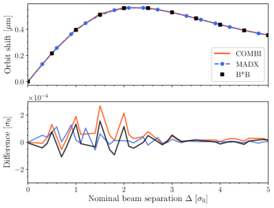
Figure 5: Top: bunch-centroid displacement $\delta^{bb}_{iB}$ due to the beam-beam deflection during a simulated vdM scan, as predicted by COMBI, MAD-X and B*B. The bunch parameters are listed in the right column of Table 1. The horizontal axis is the nominal beam separation in units of the unperturbed transverse beam size $\sigma_{0}$. Bottom: difference between the simulated orbit shift and that calculated analytically using Eqs. (14)-(15), in units of $\sigma_{0}$. The wiggles reflect the combination of a finite sampling step ($0.2\,\sigma_{0}$) and of numerical noise.

During a luminosity-calibration session, the bunches typically collide at more than one IP (Sec. 4.6); however performing simultaneous beam-separation scans at different IPs is carefully avoided. Under these conditions and to an excellent approximation, the orbit shifts associated with slightly misaligned collisions at a non-scanning IP remain static during a beam-separation scan at another IP. Their impact on the beam separation at the scanning IP is therefore expected to remain constant during the scan, and has been neglected in the simulations reported in this paper.

3.5.2 Impact of amplitude-dependent $\beta$-beating effects in the Gaussian-bunch approximation

The beam-separation dependence of the transverse RMS beam-size ratio (squared for easier interpretation in terms of luminosity) is presented in Fig. 4. The results of B*B and COMBI agree to better than $2\times 10^{-4}$.

At $\Delta=0$, both predict a decrease in beam-size squared (or equivalently an increase in head-on luminosity) about half of that obtained using MAD-X. This is remarkably consistent with Eq. (22): in MAD-X, all particles in the witness bunch are subject to the same quadrupole-like force as the zero-amplitude particle, while in B*B and COMBI, the slope of the beam-beam force decreases and even changes sign as the betatron amplitude increases (Fig. 3), resulting in a smaller overall change in optical demagnification at the IP.

Amplitude detuning also explains the different $\Delta$-dependence of the beam sizes, with that in MAD-X being more pronounced than in B*B and COMBI. At very large beam separation, where the electromagnetic force becomes similar to that of a distant, point-like charge, all three curves tend towards a common asymptote. As for the different evolution of the horizontal and vertical beam sizes during a scan, it simply reflects the tune-dependence apparent in, for instance, Eq. (18).

If one assumes that the optical distortions discussed above modify the transverse RMS bunch sizes at the IP without significantly affecting their initial, purely Gaussian shape, Eqs. (5)–(7) apply. The combination of the beam-beam induced orbit shift and of the optical distortions then yields the following expression for the luminosity-bias factor during a beam-separation scan in plane $i$ ($i=x,y$):

$$\frac{\mathcal{L}}{\mathcal{L}^{0}}(\Delta_{i}) = \frac{\Sigma^{0}_{x}\Sigma^{0}_{y}}{\Sigma_{x}(\Delta_{i})\Sigma_{y}(\Delta_{i})}e^{-\frac{1}{2}[(\delta_{i}/\Sigma_{i})^{2}-(\Delta_{i}/\Sigma^{0}_{i})^{2}]}$$ (23)

$$= \frac{(\sigma^{0})^{2}}{\sigma_{x}(\Delta_{i})\sigma_{y}(\Delta_{i})}e^{-\frac{1}{4}[(\delta_{i}/\sigma_{i})^{2}-(\Delta_{i}/\sigma^{0})^{2}]}$$ (24)

where $\sigma_{x,y}$, $\Sigma_{x,y}$, $\mathcal{L}$ (resp. $\sigma_{0}$, $\Sigma^{0}_{x,y}$, $\mathcal{L}^{0}$) are the RMS single-beam sizes, the inverse of the overlap integrals and the luminosity in the presence (resp. absence) of the beam-beam interaction.

Combining Eq. (24) with the beam-size ratios shown in Fig. 4 yields the beam-separation dependence of the luminosity-bias factor $[\mathcal{L}/\mathcal{L}^{0}](\Delta)$ in the Gaussian-bunch approximation, as illustrated in Fig. 6 for MAD-X (dashed blue) and COMBI (dotted grey). These curves are not simply the inverse of the beam-size ratios displayed in Fig. 4, because they include in addition the impact, at a given nominal separation, of the beam-beam induced orbit shift. At zero and moderate separation ($\Delta/\sigma_{0}<1$). the luminosity bias $[\mathcal{L}/\mathcal{L}^{0}]-1$ is positive and dominated by the dynamic-$\beta$ effect; as the separation increases, the orbit shift, which is represented by the exponential term in Eq. (23), progressively takes over.

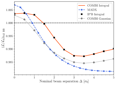
Figure 6: Beam-separation dependence of the luminosity-bias factor $[\mathcal{L}/\mathcal{L}^{0}]_{\mathrm{Full\,BB}}$ during a simulated horizontal  scan. The unperturbed beams are assumed to be round and perfectly Gaussian; their parameters are listed in the right column of Table 1. The horizontal axis is the nominal beam separation in units of the unperturbed transverse beam size $\sigma_{0}$. The MAD-X (dashed blue) and COMBI (dotted grey) curves are valid only in the Gaussian-bunch approximation (Sec. 3.5.2); the COMBI (red curve) and the B*B markers (black squares) are obtained from the overlap integrals of the multiparticle distributions (Sec. 3.5.3).

3.5.3 Impact of optical distortions on the beam-beam overlap integral

If the transverse-density distributions are sufficiently distorted by the non-linearity of the beam-beam force, the Gaussian-bunch approximation encapsulated in Eqs. (23)–(24) is no longer valid, and the luminosity bias must be calculated numerically from the beam–separation-dependent overlap integrals of the macroparticle distributions. To this effect, an integrator module, detailed in Appendix B, has been developed for COMBI; B*B provides an equivalent functionality [8]. The resulting beam-separation dependence of the luminosity-bias factor is shown by the red curve and the black markers in Fig. 6. At each simulated scan step (indicated by the markers), B*B and COMBI agree to better than $2\times 10^{-4}$; the difference is not systematic, but fluctuates around zero. The difference between the Gaussian-bunch approximation and the numerically calculated overlap integral demonstrates that the non-Gaussian tails induced by the beam-beam interaction have a significant impact on the luminosity as soon as $\Delta/\sigma_{0}\geq 0.2$. The excellent agreement between the two multiparticle simulations also demonstrates that strong-strong beam-beam effects, that are modeled by COMBI but not by B*B, remain negligible in the low beam-beam parameter regime considered here.

Since the predicted orbit effect is identical in all simulations (Fig. 5), the differences between MAD-X on the one hand (Fig. 6, dashed blue curve), and B*B/COMBI on the other (black markers/red curve), is entirely associated with optical distortions. At zero separation, the difference is entirely explained by amplitude detuning (Eq. (22)); once the separation increases, beam–beam-induced non-Gaussian tails play a growing role, as illustrated by the difference between the red and grey curves.

In the context of the beam-beam correction strategy outlined in Sec. 2.3, it is convenient to separate the full luminosity bias presented in Fig. 6 into its optical-distortion and orbit-shift components. The luminosity-bias factor associated with optical distortions and denoted by $[\mathcal{L}/\mathcal{L}^{0}]_{\mathrm{Opt}}$ is defined as the ratio, scan step by scan step, of the full luminosity-bias factor $[\mathcal{L}/\mathcal{L}^{0}]_{\mathrm{Full\,BB}}$ and of the bias factor $[\mathcal{L}/\mathcal{L}^{0}]_{\mathrm{Orb}}$ associated with the orbit shift:

$$[\mathcal{L}/\mathcal{L}^{0}]_{\mathrm{Opt}}(\Delta)=\frac{[\mathcal{L}/\mathcal{L}^{0}]_{\mathrm{Full\,BB}}(\Delta)}{[\mathcal{L}/\mathcal{L}^{0}]_{\mathrm{Orb}}(\Delta)}$$ (25)

Its beam-separation dependence is presented in Fig. 7. While MAD-X overestimates the dynamic-$\beta$ effect at zero separation, it strongly underestimates the optical distortions at medium and large beam separations. Since all models predict the same orbit effect, and since the optical distortions and the orbit effect impact the overlap integrals in opposite ways, their mutual cancellation is stronger in B*B and COMBI than in MAD-X, resulting in a net overall beam-beam correction of significantly smaller magnitude. This will be discussed quantitatively in Sec. 4.

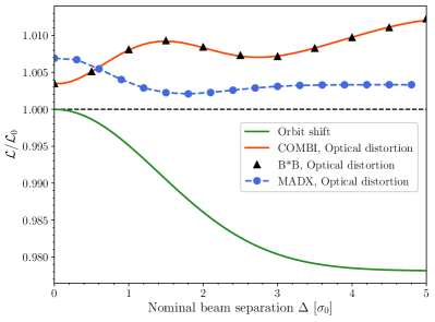
Figure 7: Beam-separation dependence, during a simulated horizontal  scan, of the luminosity-bias factor $[\mathcal{L}/\mathcal{L}^{0}]_{\mathrm{Opt}}$ associated with the optical distortions, and of that induced by the beam-beam orbit effect ($[\mathcal{L}/\mathcal{L}^{0}]_{\mathrm{Orb}}$). The unperturbed beams are assumed to be round and perfectly Gaussian; their parameters are listed in the right column of Table 1. The horizontal axis is the nominal beam separation in units of the unperturbed transverse beam size $\sigma_{0}$. The MAD-X (dashed blue line with markers), weak-strong B*B (black triangles) and strong-strong COMBI (red curve) optical-distortion curves are obtained by dividing the corresponding full beam-beam bias factor shown in Fig. 6 by that predicted analytically for the orbit effect alone (green curve).

3.5.4 Beam-parameter dependence of beam-beam corrections

The results in Figs. 6 and 7 were obtained using the reference parameter set in the right column of Table 1. This corresponds to a beam-beam parameter $\xi=2.59\times 10^{-3}$, at the low end of the $\xi$ range explored during  scans at $\sqrt{s}=13$ TeV. The cross-validation of B*B and COMBI was therefore repeated with a larger bunch current and a smaller emittance, both typical of routine physics running and corresponding to a beam-beam parameter value well beyond the  range. The beam-separation dependence of the optical-distortion luminosity-bias factor at these two $\xi$ values is presented in Fig. 8. While in perfect agreement at low $\xi$, the two codes exhibit hints of a small but systematic difference in the high-$\xi$ regime when the beam separation becomes large enough. This discrepancy is attributed to the fact that B*B is intrinsically a weak-strong model, and therefore cannot account for coherent bunch oscillations, contrarily to COMBI. This interpretation is confirmed by the comparison of the tune spectra predicted by the two packages: even in the vdM regime, a $\pi$-mode peak is apparent in the COMBI spectrum, but is missing (as it should be) from the B*B spectrum.

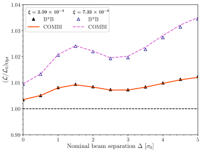
Figure 8: Beam-separation dependence, during a simulated horizontal  scan, of the luminosity-bias factor $[\mathcal{L}/\mathcal{L}^{0}]_{\mathrm{Opt}}$ associated with optical distortions, for the  reference parameter set ($\xi=2.59\times 10^{-3}$, solid red curve and black filled triangles), and for a beam-beam parameter typical of routine physics running ($\xi=7.33\times 10^{-3}$, dashed purple curve and blue open triangles). The COMBI (B*B) results are shown by the straight-line segments (markers). The horizontal axis is the nominal beam separation in units of the unperturbed transverse beam size $\sigma_{0}$.

Quantitatively, it turns out that throughout the regime and even in the high-$\xi$ case considered here, the discrepancy is of no practical significance. Since it manifests itself only in the tails of the beams ($\Delta>2\sigma_{0}$), where the particle density is low, the difference, between B*B and COMBI, in beam–beam-induced distortions has only a very small impact on the integral of the scan curves, i.e. on the perturbed transverse convolved beam sizes (Eq. (4)). This can be quantified using the methodology that will be presented in Sec. 4.2.4. For the high-$\xi$ setting illustrated in Fig. 8, the difference between B*B and COMBI translates into a systematic uncertainty of 0.04% on the absolute luminosity scale. In typical scans, where $\xi$ is lower by a factor of about 1.5, the inconsistency becomes negligible; there the two simulation codes remain in more than adequate agreement, validating the use of the less resource-intensive B*B package for parameterizing beam-beam corrections to  calibrations.

4 Calculated impact of beam-beam dynamics on luminosity calibrations

4.1 Methodology

The beam-beam biases affecting a  calibration are accounted for by correcting the luminosity-scan curves, one bunch pair at a time, according to the procedure outlined in Sec. 2.3. While the orbit shift (Sec. 2.3.1) can be calculated analytically, correcting for optical distortions (Sec. 2.3.2) requires the knowledge of the beam-separation dependence of the luminosity-bias factor $[\mathcal{L}/\mathcal{L}^{0}]_{\mathrm{Opt}}$, such as that illustrated in Fig. 8. The latter can be obtained by running B*B or COMBI with, as input:

• the interaction-region (IR) configuration (beam energy, nominal or measured $\,\beta^{*}$ and crossing-angle values);

• the unperturbed tunes $\text{Q}_{x}$ and $\text{Q}_{y}$ (or equivalently the unperturbed fractional tunes $\text{q}_{x}$ and $\text{q}_{y}$), i.e. the values of the horizontal and vertical tunes with the beam-beam interaction switched off at the IP where the simulated scans are taking place. Physically, these correspond to the tune values that would be measured, for the bunch pair under study, before the beams are brought into collision at the scanning IP considered;

• the measured parameters of the bunch pair under study: bunch population, horizontal and vertical beam sizes or emittances, as well as the bunch length in case of a non-zero nominal crossing angle.

Since  calibrations must be performed on a bunch-by-bunch basis, with possibly over 100 colliding-bunch pairs and typically five to ten $x$-$y$ scan pairs per scan session and per IP, the approach sketched above can become unwieldy from the computing viewpoint. This motivated the development of a much lighter technique, based on the fact that at least in the  regime and under some simplifying assumptions, beam-beam biases, to a very good approximation, scale almost linearly with the beam-beam parameter $\xi$. This makes it possible to construct a simple polynomial parameterization of the luminosity-bias curves, that is extracted from B*B or COMBI simulations over a grid in beam-parameter space and is applicable to most cases of practical interest for $pp$  calibrations at the LHC. The impact of violating the underlying assumptions is accounted for either by a contribution to the systematic uncertainty that is associated with the beam-beam correction procedure, or, in the case of multi-IP effects, by a simulation-guided adjustment to the parameterized correction.

Some cases do not lend themselves to the parameterization technique, such as off-axis scans, diagonal scans, or  calibrations performed with a large crossing angle (which is unavoidable at the LHCb IP).

An off-axis scan is a horizontal (or vertical) beam-separation scan where the beams are partially separated in the non-scanning plane, i.e. in the vertical (or horizontal) direction. A diagonal scan is one in which the beams are scanned transversely along an inclined straight line in the $x$-$y$ plane, rather than only along either the $x$ or the $y$ axis. Such “generalized”, one-dimensional scans are sometimes used to measure and correct for non-factorization effects [13, 35, 36]. While the orbit-shift correction can still be calculated analytically using a more general form of the Bassetti-Erskine formula, the increased dimensionality of the parameter space makes it impractical to invest in general enough and precise enough a parameterization of optical-distortion effects. In such a case, deriving the corrections from a large set of fully simulated scans, labor- and CPU-intensive as it may be, appears more tractable by comparison.

Allowing non-zero crossing angles also increases the dimensionality of the parameter space, with similar implications. Therefore, except where explicitly stated otherwise, the results offered in the remainder of this report are restricted to the zero (or moderate) crossing-angle case, which covers the needs of the ATLAS and CMS experiments (as well as those of ALICE, at the cost of a slight increase in systematic uncertainty).

This Section is organized as follows. The parameterization approach mentioned above is described in Sec. 4.2. The associated “fully symmetric Gaussian-beam configuration” assumes that in the absence of any beam-beam interaction, the colliding bunches in beam 1 and beam 2:

• can be modeled by factorizable transverse-density distributions, and exhibit a single-Gaussian profile in all three dimensions. The impact of violating this assumption is evaluated in Sec. 4.3;

• are round in the transverse plane ($\sigma_{xB}=\sigma_{yB},B=1,2$). The impact of violating this assumption is evaluated in Sec. 4.4;

• intersect at zero crossing angle. The impact of violating this assumption is evaluated in Sec. 4.5;

• collide only at the IP where beam-separation scans are performed. The impact of violating this assumption is evaluated in Sec. 4.6;

• are beam-beam symmetric, i.e. equally populated ($n_{1}=n_{2}$), of the same transverse size ($\sigma_{i,1}=\sigma_{i,2}$, $i=x,y$), and therefore subject to the same beam-beam parameter ($\xi_{i,1}=\xi_{i,2},i=x,y$). The impact of violating these assumptions is evaluated in Sec. 4.7.

4.2 Beam-beam correction procedure in the fully symmetric Gaussian-beam configuration

The parametrization strategy relies on the fact that at fixed tunes, beam-beam induced biases to the visible cross-section depend only on the beam-beam parameter $\xi$ (Sec. 4.2.1). The simulated $\xi$- and tune-dependence of the luminosity-bias functions (Sec. 4.2.2) leads to parameterizing them by second-order polynomials that can be used, in the context of the beam-beam correction procedure of calibrations, as a proxy for full-fledged B*B or COMBI simulations (Sec. 4.2.3). Combining these parameterized bias functions with hypothetical -scan curves devoid of fitting biases and of step-to-step fluctuations provides robust and intuitive insight into the magnitude and beam-conditions dependence of beam-beam corrections to luminosity calibrations (Sec. 4.2.4).

4.2.1 Validation of the scaling hypothesis

To characterize the scaling properties (or lack thereof) of beam-beam biases during vdM scans, pairs of horizontal and vertical beam-separation scans were generated under the assumptions above using B*B. The beam-beam parameter spanned the range $\xi\sim 0.002-0.008$, thereby covering from  scans with low-brightness proton beams at the low end, to conditions slightly above routine physics running at the high end. The input beam energies, bunch populations, emittance and $\,\beta^{*}$ values were chosen to be representative of  scans during LHC Runs 1 and 2 (Sec. 2.2); also included was a high-$\xi$ setting representative of Run-2 high-luminosity physics running. The unperturbed fractional tunes were constrained to satisfy $\text{q}_{y}=\text{q}_{x}+0.010$ so as to reflect routine LHC collision settings.

The primary output of the simulation is the beam-separation dependence of the luminosity-bias factor $[\mathcal{L}/\mathcal{L}^{0}]_{\mathrm{Full\,BB}}$. An example is presented in Fig. 9, with a value of $\xi$ chosen to lie roughly in the middle of the  range (Table 1). The orbit-shift bias factor $[\mathcal{L}/\mathcal{L}^{0}]_{\mathrm{Orb}}$ (green squares) is computed analytically:

$$[\mathcal{L}/\mathcal{L}^{0}]_{\mathrm{Orb}}(\Delta)=e^{-\frac{1}{2}[(\delta_{i}/\Sigma_{R})^{2}-(\Delta/\Sigma_{R})^{2}]}$$ (26)

where $\Delta$ is the nominal separation in the scanning plane, $\delta_{i}$ is computed using Eqs. (14) to (16), and $\Sigma_{R}=\sqrt{\Sigma^{0}_{x}\,\Sigma^{0}_{y}}$ is the unperturbed, round beam-equivalent convolved beam size that in this particular case satisfies $\Sigma_{R}=\Sigma^{0}_{x}=\Sigma^{0}_{y}=\sqrt{2}\,\sigma_{0}$. The optical-distortion bias factor $[\mathcal{L}/\mathcal{L}^{0}]_{\mathrm{Opt}}$ (red triangles) can then be calculated using Eq. (25).

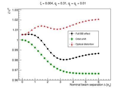
Figure 9: Beam-separation dependence, during a simulated horizontal  scan, of the luminosity-bias factor associated with the beam-beam orbit shift only (green squares), the optical distortions only (red triangles), and their combination (black circles). The horizontal axis is the nominal beam separation in units of the unperturbed transverse beam size $\sigma_{0}$. The beams satisfy the assumptions listed in Sec. 4.1. The input unperturbed-tune and beam-beam parameter values are indicated at the top; the other relevant parameters are $E_{B}=6.5$ TeV, $\,\beta^{*}=19.2$ m and $\epsilon_{N}=2.6\,\mu$m$\cdot$rad. The points are the results of the simulation; the lines are intended to guide to eye.

For given values of $\text{q}_{x}$ and $\text{q}_{y}$, beam–beam-induced distortions scale with the beam-beam parameter, in the sense that they depend only on $\xi$. This can be proven mathematically, both for the orbit shift (Eqs. (14)-(15)) and for the dynamic-$\beta$ effect at zero separation (Eq. (18)). That this remains true at any beam separation, within the constraints of the fully symmetric beam configuration and over the $\xi$ range specified above, can only be demonstrated by simulation. To this effect, luminosity-bias curves such as those presented in Fig. 9 were compared for different combinations of bunch populations, beam energies, $\,\beta^{*}$ and emittance values that all correspond to a given value of $\xi$; they were found to be identical within the statistics of the simulation.

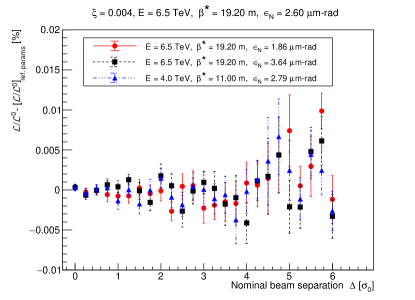
Figure 10: Beam-separation dependence, during simulated horizontal  scans, of the difference between the luminosity-bias factor (full beam-beam effect) calculated for the collision parameters shown in the legend, and that computed using the reference parameters (Fig. 9, black circles) listed at the top of the present figure. For each parameter set, the bunch intensity is adjusted such that the value of $\xi$ remains the same. The error bars are explained in the text.

An example is presented in Fig. 10, which displays the difference, at each scan step, between the luminosity-bias factor computed for three distinct sets of beam parameters, and that associated with the parameters used in Fig. 9; all four parameter sets correspond to $\xi=0.004$. The error bars represent the statistical uncertainty associated with the randomization of initial conditions in the B*B code [8]; they are computed as the error on the mean over eight different runs, with different random seeds, for each beam separation and each parameter set. The differences in luminosity-bias values between the four beam-parameter sets and the reference set are statistically consistent with zero, and never exceed $10^{-4}$. The exercise was repeated for a range of $\xi$ values, leading to the conclusion that at fixed $\text{Q}_{x}$ and $\text{Q}_{y}$, the luminosity-bias curves indeed depend only on $\xi$, to better than $10^{-4}$ on the absolute luminosity scale.

4.2.2 Beam-beam parameter and tune dependence of the optical-distortion correction

The combined beam-separation and $\xi$ dependence of the luminosity-bias factor $[\mathcal{L}/\mathcal{L}^{0}]_{\mathrm{Opt}}$ is illustrated in Fig. 11. The simulations shown span the full beam-beam parameter range ($2.04\times 10^{-3}\leq\xi\leq 7.83\times 10^{-3}$), and are carried out at the nominal LHC tune settings ($\text{Q}_{x}=64.31$, $\text{Q}_{y}=59.32$). A similar $\xi$-dependence is observed for $[\mathcal{L}/\mathcal{L}^{0}]_{\mathrm{Full\,BB}}$ and $[\mathcal{L}/\mathcal{L}^{0}]_{\mathrm{Orb}}$ (not shown). The beam-beam parameter dependence of all three variables at fixed nominal separation is found to be well modeled by a second-order polynomial of $\xi$, the coefficients of which depend on the nominal separation.

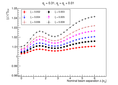
Figure 11: Beam-separation dependence, during simulated horizontal  scans, of the luminosity-bias factor $[\mathcal{L}/\mathcal{L}^{0}]_{\mathrm{Opt}}$ associated with optical distortions, for several values of the beam-beam parameter $\xi$. The horizontal axis is the nominal beam separation in units of the unperturbed transverse beam size $\sigma_{0}$. The beams satisfy the assumptions listed in Sec. 4.1. The input unperturbed fractional-tune values are indicated at the top. The points are the results of the simulation; the lines are intended to guide the eye.

Since both the orbit shift (Eq. (15)) and the dynamic-$\beta$ effect (Eq. (18)) depend on the unperturbed tunes, and as part of investigating the systematic uncertainties associated with beam-beam corrections, their sensitivity to the input tune values was characterized by extending the above-described simulations to an area in the ($\text{q}_{x}$, $\text{q}_{y}$) plane that encompasses the full range of operational tune settings and of beam-beam tune shifts expected during sessions. Horizontal and vertical beam-separation scans were simulated, for several values of $\xi$, over a grid bounded by $0.2975<\text{q}_{x}<0.3100$, with the vertical unperturbed fractional tune set to $\text{q}_{y}=\text{q}_{x}+\delta_{\mathrm{q}}$ where $\delta_{\mathrm{q}}=0.0075,0.0100,0.0125$.

The combined beam-separation and tune dependence of the luminosity-bias factor $[\mathcal{L}/\mathcal{L}^{0}]_{\mathrm{Opt}}$ is illustrated in Fig. 12 for $\xi=7.83\times 10^{-3}$. For a given nominal separation, the lower the tunes, the more they approach the quarter integer, and therefore the smaller (i.e. the closer to unity) the optical-distortion bias factor becomes [4]. Similarly, the lower the tunes, the smaller (i.e. the further away from unity) the orbit-shift bias factor $[\mathcal{L}/\mathcal{L}^{0}]_{\mathrm{Orb}}$ (not shown), albeit with a weaker tune dependence. As a result, the tune dependence of the full beam–beam-bias factor $[\mathcal{L}/\mathcal{L}^{0}]_{\mathrm{Full\,BB}}$ is slightly steeper than that associated with optical distortions only: the lower the tunes, the faster $[\mathcal{L}/\mathcal{L}^{0}]_{\mathrm{Full\,BB}}$ drops in magnitude (Fig. 13), and therefore the larger the overall beam-beam correction to the luminosity scale. In addition, the lower the tunes, the less the optical distortions contribute to the overall beam-beam bias to $\,\sigma_{\mathrm{vis}}$.

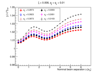
Figure 12: Beam-separation dependence, during simulated horizontal  scans, of the luminosity-bias factor $[\mathcal{L}/\mathcal{L}^{0}]_{\mathrm{Opt}}$ associated with optical distortions, for several values of the unperturbed fractional tunes ($\text{q}_{x}$, $\text{q}_{y}$). The horizontal axis is the nominal beam separation in units of the unperturbed transverse beam size $\sigma_{0}$. The beams satisfy the assumptions listed in Sec. 4.1. The input $\xi$ value is indicated at the top. For each curve, the value of the horizontal tune is indicated in the legend; the value of the vertical tune is set to $\text{q}_{y}=\text{q}_{x}+0.01$. The points are the results of the simulation; the lines are intended to guide the eye.

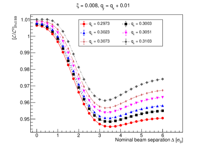
Figure 13: Beam-separation dependence, during simulated horizontal  scans, of the luminosity-bias factor $[\mathcal{L}/\mathcal{L}^{0}]_{\mathrm{Full\,BB}}$ associated with the full beam-beam effect, for several values of the unperturbed fractional tunes ($\text{q}_{x}$, $\text{q}_{y}$). The horizontal axis is the nominal beam separation in units of the unperturbed transverse beam size $\sigma_{0}$. The beams satisfy the assumptions listed in Sec. 4.1. The input $\xi$ value is indicated at the top. For each curve, the value of the horizontal tune is indicated in the legend; the value of the vertical tune is set to $\text{q}_{y}=\text{q}_{x}+0.01$. The points are the results of the simulation; the lines are intended to guide the eye.

4.2.3 Practical implementation of parameterized beam-beam corrections

Concretely, given a measured -scan curve such as that displayed in Fig. 1 (bottom), the beam-beam correction procedure can be implemented as follows.

1. At each scan step in the $i$ scanning plane ($i=x,y$), correct the nominal separation $\Delta_{i}$ for the deflection-induced separation shift $\delta^{bb}_{i}$, as detailed in Sec. 2.3.1, using Eqs. (14)–(16).

2. At each scan step in the $i$ scanning plane, correct the measured rate $R_{i}(\Delta_{i})$ for the optical-distortion bias as detailed in Sec. 2.3.2, using Eq. (17). The beam-separation dependence of the luminosity-bias factor $[\mathcal{L}/\mathcal{L}^{0}]_{\mathrm{Opt}}$ is either extracted directly from a set of B*B or COMBI simulations, or, if the assumptions listed in Sec. 4.1 can be considered valid, simply computed using the polynomial parameterization described below. The latter is valid only for on-axis, one-dimensional scans with zero crossing angle; other configurations, and in particular off-axis one-dimensional scans as well as two-dimensional grid scans in the $(\delta_{x},\delta_{y})$ beam-separation plane, require dedicated simulations.

The simulations described in Sec. 4.2.2 were used to parameterize the optical-distortion luminosity-bias factor $[\mathcal{L}/\mathcal{L}^{0}]_{\mathrm{Opt}}$ in bins of normalized nominal separation over the range $0\leq\Delta_{i}/\sigma_{0}\leq 6$, separately for $x$ and $y$ scans, by polynomials of the form

$$[\mathcal{L}/\mathcal{L}^{0}(\xi_{R},\text{q}_{x},\text{q}_{y})]_{k} = p_{0k}$$ (27)

$$+ p_{1k}\,\xi_{R}+p_{2k}\,\text{q}_{x}+p_{3k}\,\text{q}_{y}$$

$$+ p_{4k}\,\xi_{R}^{2}+p_{5k}\,\text{q}_{x}^{2}+p_{6k}\,\text{q}_{y}^{2}$$

$$+ p_{7k}\xi_{R}\text{q}_{x}+p_{8k}\,\xi_{R}\,\text{q}_{y}$$

$$+ p_{9k}\,\text{q}_{x}\,\text{q}_{y}\,.$$

Here the index $k$ ($k=$ 1, 25) labels the nominal-separation bin in the scanning plane considered. The round-beam equivalent beam-beam parameter $\xi_{R}$ is defined as

$$\xi_{R}=\frac{nr_{0}\,\beta^{*}}{4\pi\gamma\sigma_{R}^{2}}\,,$$ (28)

where the single-beam transverse RMS beam size $\sigma_{0}$ in Eq. (13) is approximated by its measured round-beam equivalent $\sigma_{R}=\sqrt{\Sigma_{x}\Sigma_{y}/2}$, thereby partially accounting for a potential ellipticity of the beams at the IP. The input fractional-tune values ($\text{q}_{x}$, $\text{q}_{y}$) are those of the unperturbed tunes defined in Sec. 4.1. In the case where bunches collide only at the IP where the scan is taking place, i.e. remain fully separated, transversely and/or longitudinally, at the other three IPs, these unperturbed tunes are identical to the nominal LHC tunes, or equivalently to the values one would measure before the beams are put in collision at the scanning IP. If, however, some bunches also collide at one or more other IPs, the unperturbed tunes input to the parameterization for those bunches must take into account the beam-beam tune shift arising from collisions at non-scanning IPs; a prescription to this effect is offered in Sec. 4.6.

The parameterization above, that amounts to a second-order Taylor expansion in $\xi_{R}$, $\text{q}_{x}$ and $\text{q}_{y}$, was found sufficient to approximate the exact simulation results to better than $10^{-3}$ on $[\mathcal{L}/\mathcal{L}^{0}]$ over most of the grid of simulated points in ($\xi$, $\text{q}_{x}$, $\text{q}_{y}$, $\Delta$) space.. The function defined by Eq. (27) is linear in all 10 parameters $p_{lk}$. In each nominal-separation bin $k$, the set of parameters $p_{0k},\dots,p_{9k}$ is determined by a weighted linear least-square fit. A smooth dependence of $[\mathcal{L}/\mathcal{L}^{0}]$ on the nominal separation, for given values of $\xi_{R}$, $\text{q}_{x}$ and $\text{q}_{y}$, can be achieved by, for instance, cubic spline interpolation between adjacent separation bins. Parameterizations based on the same functional form were also constructed for the orbit-shift and full beam-beam bias factors $[\mathcal{L}/\mathcal{L}^{0}]_{\mathrm{Orb}}$ and $[\mathcal{L}/\mathcal{L}^{0}]_{\mathrm{Full\,BB}}$, and achieved similar numerical accuracy.

Tabulated values of the parameters $p_{lk}$ in separation steps of $0.25$ in $\Delta/\sigma_{R}$, for both vertical and horizontal scans and over the full range of $\xi_{R}$ and tune values defined earlier, have been made available to all LHC experimental Collaborations. The optical-distortion parameters, which are the most useful, are documented in Appendix C, and are publicly accessible in computer-readable form [37].

4.2.4 Separation-integrated estimates of beam-beam corrections to vdM calibrations

The beam-beam correction procedure detailed in the preceding Section is designed to be applied to measured -scan curves, one scan step at a time. One then extracts the beam-beam corrected peak rate and convolved beam sizes needed to calculate the visible cross-section (Eq. (10)) using a carefully chosen fit function. More often than not, the latter must diverge from a perfect Gaussian in order to faithfully model the data over the full beam-separation range.

In order to provide consistency checks on this intricate analysis chain, as well as a physically intuitive, albeit approximative, breakdown of the impact of individual beam-beam effects on the luminosity calibration under study, the same procedure can be applied to an $x$-$y$ pair of hypothetical beam-separation scan curves, that suffer from no statistical fluctuations and that, in the $\xi_{R}\rightarrow 0$ limit would be perfectly Gaussian:

$$\mathcal{L}^{0}(\Delta)\propto\frac{1}{4\pi\sigma_{0}^{2}}\exp\left(-\frac{\Delta^{2}}{4\sigma_{0}^{2}}\right)\,.$$

Here and in the remainder of this paper, the “0” index indicates a “nominal” quantity, i.e. one for which beam-beam effects have been fully turned off in the simulation.

At a given nominal separation $\Delta_{i}$ in scanning plane $i$ ($i=x,y$), and with the beams transversely centered on each other in the non-scanning plane, the luminosity in the presence of, say, the full beam-beam effect is then calculated as

$$\mathcal{L}(\Delta_{i})=\mathcal{L}^{0}(\Delta_{i})\times[\mathcal{L}/\mathcal{L}^{0}]_{\mathrm{Full\,BB}}(\Delta_{i})$$ (29)

with $[\mathcal{L}/\mathcal{L}^{0}]_{\mathrm{Full\,BB}}(\Delta_{i})$ provided by the parametrization detailed in Sec. 4.2.3, with input parameters representative of the actual beam conditions during the scans under study. The impact of either the orbit shift or the optical distortions alone can be evaluated by substituting $[\mathcal{L}/\mathcal{L}^{0}]_{\mathrm{Orb}}(\Delta_{i})$ or $[\mathcal{L}/\mathcal{L}^{0}]_{\mathrm{Opt}}(\Delta_{i})$ for $[\mathcal{L}/\mathcal{L}^{0}]_{\mathrm{Full\,BB}}(\Delta_{i})$ in Eq. (29).

One then defines “figures of merit” (FoMs) that characterize the impact of beam-beam effects on observables.

1. The peak-rate bias factor characterizes the dynamic-$\beta$ effect at zero beam separation:

   $$\mu_{pk}/\mu_{pk}^{0}=\frac{\mathcal{L}(\Delta_{i}=0)}{\mathcal{L}^{0}(\Delta_{i}=0)},$$ (30)

   and is sensitive to optical distortions only.

2. The beam-size bias factors characterize, in each plane, the beam-beam impact on the convolved transverse beam size:

   $$\Sigma_{i}/\Sigma_{i}^{0}~{}(i=x,y),$$ (31)

   where the overlap integrals

   $$\Sigma_{i} = \frac{1}{\sqrt{2\pi}}~{}\frac{\int\mathcal{L}(\Delta_{i})\,\mathrm{d}\Delta_{i}}{\mathcal{L}(\Delta_{i}=0)}$$ (32)

   $$\Sigma_{i}^{0} = \frac{1}{\sqrt{2\pi}}~{}\frac{\int\mathcal{L}^{0}(\Delta_{i})\,\mathrm{d}\Delta_{i}}{\mathcal{L}^{0}(\Delta_{i}=0)}$$ (33)

   are calculated numerically, with their integrands smoothed by cubic-spline interpolation.

3. The $\,\sigma_{\mathrm{vis}}$-bias factor characterizes the beam-beam impact on the absolute luminosity scale, and is given by the product of the previous three FoMs:

   $$\,\sigma_{\mathrm{vis}}/\,\sigma^{0}_{\mathrm{vis}} = (\mu_{pk}/\mu_{pk}^{0})$$ (34)

   $$\times(\Sigma_{x}/\Sigma_{x}^{0})\times(\Sigma_{y}/\Sigma_{y}^{0})\,.$$

As an illustration, Fig. 14 displays the beam-beam parameter dependence of the peak-rate bias factor for the full beam-beam effect (black circles), the orbit shift only (green squares), and the optical distortion only (red triangles). Since at zero separation there is no orbit shift, only optical distortions matter in this case.

The evolution of the horizontal beam-size bias factor is presented in Fig. 15. While orbit shifts, if left uncorrected, result in an underestimate of $\Sigma_{x}$ and $\Sigma_{y}$, optical distortions have the opposite effect, resulting in a partial cancellation of the bias.

This is even more apparent in the visible-cross-section bias curves (Fig. 16). While the full beam-beam effect on the visible cross section remains below $1\%$ over the whole $\xi$ range (black circles), individual contributions from the orbit shift (green squares) and the optical distortion (red triangles) can each lead to a $3-4\%$ bias, a clear demonstration of how much overcorrection can be expected from too approximate a treatment of optical distortions.

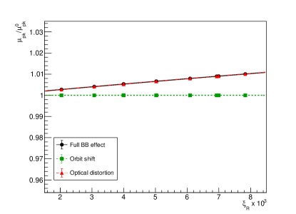
Figure 14: Dependence of the peak-rate bias factor on the beam-beam parameter, with beams colliding at the scanning IP only. The unperturbed tunes are fixed at the nominal LHC values ($\text{Q}_{x}$ = 64.31, $\text{Q}_{y}$ = 59.32). The symbols display the simulation results; the curves are described in the text. Since the orbit shift does not impact the peak-rate bias factor, the red and black symbols and curves lie exactly on top of each other.

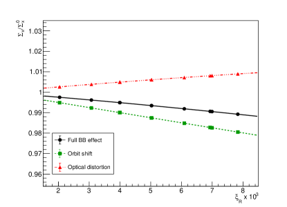
Figure 15: Dependence of the horizontal beam-size bias factor on the beam-beam parameter, with beams colliding at the scanning IP only. The unperturbed tunes are fixed at the nominal LHC values ($\text{Q}_{x}$ = 64.31, $\text{Q}_{y}$ = 59.32). The symbols display the simulation results; the curves are described in the text.

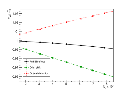
Figure 16: Dependence of the $\,\sigma_{\mathrm{vis}}$ bias factor on the beam-beam parameter, with beams colliding at the scanning IP only. The unperturbed tunes are fixed at the nominal LHC values ($\text{Q}_{x}$ = 64.31, $\text{Q}_{y}$ = 59.32). The symbols display the simulation results; the curves are described in the text.

In Figs. 14–16, the curves are fits to quadratic functions of $\xi_{R}$:

$$f(\xi_{R})_{j}=p_{0j}+p_{1j}\xi_{R}+p_{2j}\xi_{R}^{2},$$ (35)

where $j$ labels the type of correction (orbit shift only, optical distortion only, or full beam-beam). Even though the linear term is clearly dominant, a quadratic term is needed to describe the evolution of all three FoMs to satisfactory precision over the full range of beam-beam parameter values.

The impact of beam-beam effects on the absolute-luminosity scale can be expressed equivalently by either the $\,\sigma_{\mathrm{vis}}$ bias factor $\,\sigma_{\mathrm{vis}}/\,\sigma^{0}_{\mathrm{vis}}$, the visible cross-section bias $\,\sigma_{\mathrm{vis}}/\,\sigma^{0}_{\mathrm{vis}}-1$ (typically a fraction of a percent), or a multiplicative correction factor $(\,\sigma_{\mathrm{vis}}/\,\sigma^{0}_{\mathrm{vis}})^{-1}$ to the raw visible cross-section. This FoM approach, that lends itself to a simple polynomial parameterization in terms of $\xi_{R}$, $\text{q}_{x}$ and $\text{q}_{y}$, offers the advantage that its results are easy to interpret, as well as insensitive both to the quality of the fit to the measured scan curves and to rate fluctuations, from one scan step to the next, due for instance to counting statistics or beam-position jitter. This technique also simplifies the evaluation of some of the systematic uncertainties discussed in the remainder of this chapter. It is, however, not recommended for determining the central value of the beam-beam correction on real data, since it ignores the deviations of the actual scan curves from a perfect Gaussian.

4.3 Impact of non-Gaussian unperturbed transverse beam profiles

All the simulation results presented in this report so far make the explicit assumption that in the absence of the beam-beam interaction at the scanning IP, the unperturbed transverse beam profiles, i.e. the particle density functions $\hat{\rho}_{B}(x,y)$ ($B=1,2$) in Eq. (1), can be perfectly modeled by the uncorrelated $x$-$y$ product of two single, one-dimensional Gaussians. Should this not be the case, the beam-separation dependence of the luminosity-bias curves will deviate from that presented in Sec. 4.2. This is due both to the modified spatial dependence of the field generated by the source bunch, and to the fact that the fraction of particles in the witness bunch that experience a given electromagnetic kick is different from that in the pure-Gaussian case.

Both B*B and COMBI accept as input unperturbed transverse-density distributions, functional forms that are more general than a single Gaussian. In order to assess the potential impact, on beam-beam corrections, of non-Gaussian beams, a realistic model of $\hat{\rho}_{B}(x,y)$ is needed, or at least one that represents the “worst-case” deviation from the ideal Gaussian shape while remaining representative of actual beam conditions during -calibration sessions at the LHC (Sec. 4.3.1). Taking into account potentially non-factorizable unperturbed density distributions requires a minor generalization of the beam-beam correction formalism (Sec. 4.3.2). While the influence of non-Gaussian tails on the beam-separation dependence of the luminosity-bias factors appears sizeable, the resulting bias on the beam-beam corrections to the visible cross-section remains moderate enough to be treated as a systematic uncertainty (Sec. 4.3.3).

4.3.1 Single-bunch models

In a hadron collider, transverse-density distributions cannot be calculated from first principles, and existing beam-profile monitors, such as wire scanners or synchrotron-light telescopes, have too limited a dynamic range to provide sufficiently precise beam-tail measurements. The only remaining experimental handle, therefore, is that provided by non-factorization analyses such as those described in, for instance, Refs. [13, 38, 39, 40, 41]. In this approach, the bunch-density distributions are modeled by the sum of two or three three-dimensional Gaussians. A simultaneous fit to the beam-separation dependence, during a -scan pair, not only of the luminosity but also of the position, size, shape and orientation of the luminous region, makes it possible to estimate the single-bunch parameters of each colliding-bunch pair.

In order to quantify the largest plausible impact of non-Gaussian beam profiles on the beam-beam corrections calculated in Sec. 4.2, single-bunch parameters were extracted from the results of non-factorization analyses of a 2012, a 2017 and a 2018 session. The former is representative of Run-1 conditions at the ATLAS IP, up to and including July 2012 [13], the latter two of Run-2 sessions at the CMS IP, for which “bunch tailoring” in the injector chain [13, 42] significantly reduced non-Gaussian tails. In both cases, a ”worst-case” parameter set (in terms of deviations from a perfectly Gaussian shape) was selected from the fitted parameters of the analyzed colliding-bunch pairs. In order to separate the impact of non-Gaussian profiles discussed in this Section, from that of elliptical beams (Sec. 4.4) and of beam-beam imbalance (Sec. 4.7), as well as to maximise the sensitivity of the study, in each parameter set the most non-Gaussian transverse profile is assigned to both planes and both beams.

In a first step, the particle density distribution input to B*B is chosen to be factorizable by construction, and modeled by the product of two uncorrelated double Gaussians:

$$\hat{\rho}_{B}(x,y)=\rho_{xB}(x)\,\rho_{yB}(y)$$ (36)

$$=\frac{1}{\sqrt{2\pi}}\,\left[\frac{w_{n}}{\sigma_{n}}\exp\left(-\frac{x^{2}}{2\sigma^{2}_{n}}\right)+\frac{w_{w}}{\sigma_{w}}\exp\left(-\frac{x^{2}}{2\sigma^{2}_{w}}\right)\right]$$

$$\times\frac{1}{\sqrt{2\pi}}\,\left[\frac{w_{n}}{\sigma_{n}}\exp\left(-\frac{y^{2}}{2\sigma^{2}_{n}}\right)+\frac{w_{w}}{\sigma_{w}}\exp\left(-\frac{y^{2}}{2\sigma^{2}_{w}}\right)\right]$$

where $B=1$ or 2, the labels “$n$” and “$w$” refer to the narrow and wide components of the distribution, and their relative population is constrained by $w_{w}=1-w_{n}$. The functional form reflects the assumptions of unperturbed round beams and of equal particle-density distributions ($\hat{\rho}_{1}(x,y)=\hat{\rho}_{2}(x,y)$). The three parameter sets input to the B*B simulation are listed in Table 2. The 2012 (2017) parameter set clearly results in the most (the least) non-Gaussian shape, as evidenced qualitatively by the combination of the largest (smallest) beam-size ratio $\sigma_{w}/\sigma_{n}$ and the largest (smallest) weight of the wide component $w_{w}$, and as quantified by the single-beam kurtosis computed from the parameters listed in the Table.

Date of session	July 2012	June 2018	July 2017
LHC fill number	2855	6868	6016
$E_{B}$ [TeV]	4.0	6.5	6.5
$n_{p}$ [$10^{11}$ p/bunch]	1.1	0.85	0.84
$\,\beta^{*}$ [m]	11.0	19.2	19.2
$\text{q}_{x}$, $\text{q}_{y}$	0.31, 0.32	0.31, 0.32	0.31, 0.32
$\sigma_{n}$ [$\mu$m]	57.9	85.0	84.0
$\sigma_{w}$ [$\mu$m]	115	125	116
$\sigma_{w}/\sigma_{n}$	1.99	1.47	1.38
$w_{n}$	0.634	0.670	0.840
$w_{w}=1-w_{n}$	0.366	0.330	0.160
Single-beam kurtosis $\Gamma_{2}$	1.40	0.47	0.25

Table 2: Single-bunch parameters representative of strongly non-Gaussian single-beam profiles during ATLAS and CMS $pp$ scans in 2012, 2018 and 2017. The bunches are assumed to be round and, within each parameter set separately, beam-beam symmetric, i.e. of equal brightness for beam 1 and beam 2.

The functional form chosen for $\hat{\rho}_{B}(x,y)$ makes it possible to compute analytically the unperturbed convolved transverse beam size $\Sigma^{0}$ from the values of $\sigma_{n}$, $\sigma_{w}$, $w_{n}$ and $w_{w}$, using Eq. (4): these are listed in the top half of Table 3 (rows 3 to 6). The Gaussian-equivalent single-beam size $\,\sigma^{0}_{\mathrm{SG}}$, i.e. the transverse R.M.S. width of perfectly Gaussian bunches that would yield the same unperturbed convolved beam size as the non-Gaussian bunches studied here, is given by $\,\sigma^{0}_{\mathrm{SG}}=\Sigma^{0}/\sqrt{2}$ (Eq. (6)). These definitions naturally lead to using the “Gaussian-equivalent” beam-beam parameter $\xi$, inferred from $\,\sigma^{0}_{\mathrm{SG}}$ using Eq. (13), as the common metric in which to quantify the impact of non-Gaussian tails.

Date of session	July 2012	June 2018	July 2017
Single-beam kurtosis	1.40	0.47	0.25
Factorizable density distribution: Eq. (36)
$\Sigma^{0}$ (from Eq. (4)) [$\mu$m]	107.1	137.3	125.4
$\,\sigma^{0}_{\mathrm{SG}}=\Sigma^{0}/\sqrt{2}$ [$\mu$m]	75.7	97.1	88.7
Gaussian-equivalent $\xi~{}[10^{-3}]$	6.04	3.04	3.61
Non-factorizable density distribution: Eq. (37)
$\Sigma^{0}_{F}$ (from Eq. (40)) [$\mu$m]	100.4	134.9	124.4
$\,\sigma^{0}_{\mathrm{SG}}=\Sigma^{0}_{\text{F}}/\sqrt{2}$ [$\mu$m]	71.0	95.4	88.0
Gaussian-equivalent $\xi~{}[10^{-3}]$	6.88	3.16	3.67

Table 3: Scan parameters representative of strongly non-Gaussian beam profiles during ATLAS and CMS $pp$ scans in 2012, 2018 and 2017, calculated analytically from the single-bunch parameters listed in Table 2.

4.3.2 Beam–beam-correction formalism in the presence of non-factorization

In a second step, and in order to explore the potential impact of non-factorization on beam-beam corrections, the simplest two-dimensional, non-factorizable double Gaussian:

$$\hat{\rho}_{B}(x,y)=\frac{w_{n}}{2\pi\sigma^{2}_{n}}~{}\exp\left(-\frac{x^{2}+y^{2}}{2\sigma^{2}_{n}}\right)$$

$$+\frac{w_{w}}{2\pi\sigma^{2}_{w}}~{}\exp\left(-\frac{x^{2}+y^{2}}{2\sigma^{2}_{w}}\right)$$ (37)

is chosen as an alternative density-distribution model to be input to B*B. Since by construction such a distribution cannot be expressed as the product of uncorrelated horizontal and vertical components, the concept of one-dimensional convolved beam size defined by Eq. (4) ceases to be meaningful, and only the convolved–beam-size product $[\Sigma_{x}\Sigma_{y}]_{\mathrm{2D}}$ introduced in Eq. (8) remains amenable to physical interpretation. Accordingly, the two beam-size bias factors $\Sigma_{i}/\Sigma_{i}^{0}$ ($i=x,y)$ introduced in Eqs. (31)-(33) must be replaced by the single quantity

$$\frac{[\Sigma_{x}\Sigma_{y}]_{\mathrm{2D}}}{[\Sigma_{x}\Sigma_{y}]^{0}_{\mathrm{2D}}} = \frac{\int{\mathcal{L}(\Delta_{x},\Delta_{y})\,\mathrm{d}\Delta_{x}\,\mathrm{d}\Delta_{y}}}{\int{\mathcal{L}^{0}(\Delta_{x},\Delta_{y})\,\mathrm{d}\Delta_{x}\,\mathrm{d}\Delta_{y}}}$$ (38)

$$\times\frac{\mathcal{L}^{0}(0,0)}{\mathcal{L}(0,0)}\,,$$

where the scan and the integration are carried out over a grid in the two-dimensional nominal-separation space ($\Delta_{x},\Delta_{y}$) that extends over $\pm 5\,\sigma^{0}_{\mathrm{SG}}$ in both directions. The $\,\sigma_{\mathrm{vis}}$-bias factor defined by Eq. (34) then takes the more general form

$$\,\sigma_{\mathrm{vis2D}}/\,\sigma^{0}_{\mathrm{vis2D}} = \frac{\mu_{pk}}{\mu_{pk}^{0}}\times\frac{[\Sigma_{x}\Sigma_{y}]_{\mathrm{2D}}}{[\Sigma_{x}\Sigma_{y}]^{0}_{\mathrm{2D}}},~{}~{}$$ (39)

where the subscript “$2D$” indicates that the two-dimensional formalism introduced in Eq. (8) is used throughout the analysis.

Using $\xi$ as a common metric for both the factorizable and the non-factorizable case also requires a generalization of the formula that expresses, in terms of single-beam parameters, an observable that is akin to the transverse convolved bunch size and that can be measured in a standard, one-dimensional scan. For instance, for a vertical scan with the beams centered on each other in the horizontal plane, the measured apparent convolved width is given by:

$$\Sigma_{y\text{F}}=\frac{1}{{\sqrt{2\pi}}}\frac{{\int{R_{x,y}(\delta_{x}=0,\delta_{y})\,\mathrm{d}\delta_{y}}}}{{R_{x,y}(\delta_{x}=0,\delta_{y}=0)}}~{},$$ (40)

which reduces to Eq. (4) when $\hat{\rho}(x,y)=\rho_{x}(x)\,\rho_{y}(y)$. The subscript “F” emphasizes that while measurable, this observable cannot be used in Eqs. (5) and (10) unless the density distributions are factorizable. The importance of this distinction is illustrated by the significant differences between the top half (rows 3-6) and the bottom half (rows 7-10) of Table 3: even though both sets of scan parameters are based on Table 2, their values are significantly different in the two cases, because the non-linear $x$-$y$ correlation built into Eq. (37) affects the beam-overlap integral (Eq. (1)). These differences, the size of which appears correlated with the single-beam kurtosis, are indicative of the magnitude of the non-factorization biases that can be introduced, even in the absence of the beam-beam interaction, by applying the one-dimensional, factorizable FoM formalism of Sec. 4.2.4 to non-factorizable beams. In contrast, the analysis strategy encapsulated in Eq. (39) guarantees that non-factorizable correlations embedded in the unperturbed density distributions cancel in the $\,\sigma_{\mathrm{vis2D}}$ ratio; the latter, therefore, reflects the impact of beam-beam biases only. The study of non-factorization biases proper lies beyond the scope of the present report.

4.3.3 Impact of non-Gaussian tails on beam–beam-induced biases

In the case of factorizable density distributions, the impact of non-Gaussian tails on beam-beam corrections can be visualized by comparing the beam-separation dependence of the luminosity-bias factors $[\mathcal{L}/\mathcal{L}^{0}]$ for a given set of non-Gaussian beam parameters, to that computed for perfectly Gaussian beams that in the absence of beam-beam effects, would yield the same value of the unperturbed convolved beam size $\Sigma^{0}$, and therefore the same head-on luminosity. This is illustrated in Fig. 17 for the orbit-shift effect. In the single-Gaussian case (red curve), the steeper drop of $[\mathcal{L}/\mathcal{L}^{0}]_{\mathrm{Orb}}$ with increasing separation, and its asymptotic behavior for $\Delta_{y}\geq 300\,\mu$m, indicates that at such large separations ($\Delta_{y}>4\,\sigma^{0}_{\mathrm{SG}}$), the number of particles contributing to the source field becomes negligible, so that the latter increasingly appears to the witness bunch as a point source. In the non-Gaussian case (black curve), the charge distribution is more spread out, and the interplay between the source-field distribution and the density distribution in the witness bunch produces a less intuitive separation dependence.

The situation is reversed for optical distortions (Fig. 18): the Gaussian beams are subject to larger optical distortions at large beam separation (red curve), presumably because in such configurations the tail particles in the witness bunch experience a more intense source-field gradient when close to the center of the source bunch. The tails of the non-Gaussian beams, being subject to a more diffuse source-field distribution, experience weaker gradients and correspondingly smaller optical distortions (black curve).

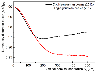
Figure 17: Beam-separation dependence, during simulated vertical  scans, of the luminosity-bias factor $[\mathcal{L}/\mathcal{L}^{0}]_{\mathrm{Orb}}$ associated with the deflection-induced orbit shift, for single-Gaussian (red) and factorizable double-Gaussian (black) bunch-density distributions that yield the same unperturbed convolved beam size. The horizontal axis is the nominal vertical beam separation. The bunch parameters are listed in the second column of Table 2 (LHC fill 2855). The beams satisfy the assumptions listed in Sec. 4.1, except (in the case of the black curve) that regarding the single-Gaussian transverse profile.

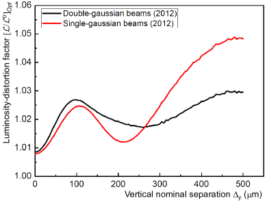
Figure 18: Beam-separation dependence, during simulated vertical  scans, of the luminosity-bias factor $[\mathcal{L}/\mathcal{L}^{0}]_{\mathrm{Opt}}$ associated with optical distortions, for single-Gaussian (red) and factorizable double-Gaussian (black) bunch-density distributions that yield the same unperturbed convolved beam size. The horizontal axis is the nominal vertical beam separation. The bunch parameters are listed in the second column of Table 2 (LHC fill 2855). The beams satisfy the assumptions listed in Sec. 4.1, except (in the case of the black curve) that regarding the single-Gaussian transverse profile.

Date of session		July 2012	June 2018	July 2017
Single-beam kurtosis		1.40	0.47	0.25
Factorizable density distribution: Eq. (36)
$\xi~{}[10^{-3}]$		6.03	3.05	3.61
$\,\sigma_{\mathrm{vis2D}}$ bias [%]:	DG	-0.27	-0.15	-0.25
	SG	-0.57	-0.22	-0.27
	DG$-$SG	0.30	0.07	0.02
DG$-$SG scaled to $\xi=5.6\cdot 10^{-3}$		0.28	0.13	0.03
Non-factorizable density distribution: Eq. (37)
$\xi~{}[10^{-3}]$		6.88	3.16	3.67
$\,\sigma_{\mathrm{vis2D}}$ bias [%]:	DG	-0.50	-0.17	-0.23
	SG	-0.64	-0.21	-0.25
	DG$-$SG	0.14	0.04	0.02
DG$-$SG scaled to $\xi=5.6\cdot 10^{-3}$		0.11	0.07	0.03

Table 4: Visible cross-section bias associated with the full beam-beam effect, calculated using B*B, for double- (DG) and single- (SG) Gaussian beams yielding the same Gaussian-equivalent beam-beam parameter $\xi$, and difference between the two (DG$-$SG). The unperturbed DG transverse-density distributions are described either by a factorizable or by a non-factorizable function; their parameters are listed in Table 2. The bunches are assumed to collide at the scanning IP only.

In the case of non-factorizable distributions, a physically intuitive graphical representation of beam-beam biases becomes impractical, since $[\mathcal{L}/\mathcal{L}^{0}]$ depends on both $\Delta_{x}$ and $\Delta_{y}$, and the curves in Figs. 17 and 18 must be replaced by surfaces.

The impact of non-Gaussian tails on the corresponding calibrations is best summarized by the $\,\sigma_{\mathrm{vis}}$-bias factors presented in Table 4. These are all computed using Eqs. (38)-(39), in order to ensure that factorizable and non-factorizable models are treated identically; it has been verified that for the factorizable models, the one-dimensional FoM formalism detailed in Sec. 4.2.4 yields the same results within 0.01% of $\,\sigma_{\mathrm{vis}}$, well within the expected accuracy of the overlap-integral calculation (Sec. 3.3). Listed in this table is the full beam-beam bias for either factorizable or non-factorizable double-Gaussian models, for the corresponding single-Gaussian model (that is factorizable by construction), as well as for their difference DG$-$SG. This difference is also listed after scaling it linearly to a common, arbitrary reference value of $\xi=5.6\cdot 10^{-3}$, that lies at the upper end of the beam-beam parameter range covered by Run-2 scans. This simple-minded procedure, inspired by the roughly linear dependence of the $\,\sigma_{\mathrm{vis}}$ bias factor on $\xi$ apparent in Fig. 16, allows direct comparisons across configurations corresponding to different values of $\xi$.

Globally, non-Gaussian tails modify the $\,\sigma_{\mathrm{vis}}$ bias by an amount that - for the models chosen here - varies from less than 10% to about half of the bias itself. Predictably enough, the larger the single-beam kurtosis, the larger the relative impact of the tails. The non-factorizable models seemingly predict a smaller influence of the tails than their factorizable counterpart; this may however depend on the particular form of $x$-$y$ correlation embedded into the specific functional form chosen for $\hat{\rho}_{B}(x,y)$. A practical proposal to translate the results listed in Table 4 into a realistic systematic uncertainty is offered in Sec. 5.2.1. Repeating the above studies using more refined single-beam models extracted from future sessions may help refine the understanding of such biases.

4.4 Impact of beam ellipticity at the interaction point

In the fully symmetric beam configuration (Sec. 4.1), the beams are round at the IP, and the beam-beam interaction can be described by a single parameter $\xi$ (Eq. 13). In the more general case where the transverse beam profile is an upright ellipse, for instance because of unequal horizontal and vertical emittances or $\,\beta^{*}$ values, the horizontal and vertical beam-beam parameters $\xi_{x}$ and $\xi_{y}$ (Eq. 12) no longer coincide, and the parametric approach described in Sec. 4.2.3 is, strictly speaking, no longer applicable.

During scans at the LHC, however, the round-beam hypothesis is only moderately violated: the measured horizontal and vertical IP-$\beta$ functions typically differ by 10% or less, the corresponding emittances by 30% at most, and the increase in projected transverse beam size associated with a non-zero crossing angle at the ALICE and LHCb IPs does not exceed 15%.

To assess the impact of beam ellipticity on beam-beam corrections, B*B is used to simulate scans over a square grid in ($\Sigma^{0}_{x}$, $\Sigma^{0}_{y}$) space (Fig. 19), with as input unperturbed beams that satisfy the assumptions listed in Sec. 4.1 except for the round-beam hypothesis. The chosen $\Sigma^{0}_{x}$ range is slightly wider than that observed during Run-2 scans at $\sqrt{s}=13$ TeV; the vertical/horizontal aspect ratio $\Sigma^{0}_{y}$/$\Sigma^{0}_{x}$ is varied from 0.7 to 1.4, corresponding to sampling the corresponding emittance ratio from 0.5 to 2.0, well beyond the range observed during -calibration sessions. The horizontal and vertical beam-beam parameters cover the range $2.6\times 10^{-3}<\xi_{x},\xi_{y}<5.1\times 10^{-3}$ (Fig. 20). The grid is chosen such that for a constant value of the round-beam equivalent beam-beam parameter $\xi_{R}$, the horizontal and vertical beam-beam parameters sample the full span allowed by the range of chosen $\Sigma^{0}_{x}$ and aspect-ratio values. For example, the group of five points at $\xi_{R}\approx 3.6\times 10^{-3}$ in Fig. 20 corresponds to the five diagonal points in Fig. 19; the residual curvature is due to the fact that the grid is built from equally spaced ($\Sigma^{0}_{x}$, $\Sigma^{0}_{y}$), rather than ($\xi_{x}$, $\xi_{y}$), values.

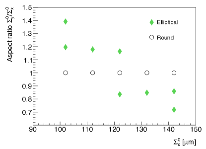
Figure 19: Grid of unperturbed transverse convolved beam sizes used to characterize the impact of beam ellipticity on beam-beam corrections, and their vertical/horizontal aspect ratio. The diamonds (circles) correspond to elliptical (round) beams. The beam energy, bunch intensity, IP-$\beta$ function and unperturbed tunes are fixed at, respectively, $E_{B}=6.5$ TeV, $n_{p}=0.777\times 10^{11}$ protons/bunch, $\,\beta^{*}=19.2$ m and $(\text{Q}_{x},\text{Q}_{y})=(64.31,59.32)$.

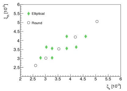
Figure 20: Grid of beam-beam parameter values used to characterize the impact of beam ellipticity on beam-beam corrections. The diamonds (circles) correspond to elliptical (round) beams. The horizontal axis shows the value of $\xi_{x}$ defined by Eq. (12), the vertical axis the corresponding round-beam equivalent parameter $\xi_{R}$ defined by Eq. (28).

The resulting peak-rate, beam-size and visible cross-section bias factors (Eqs. (30)–(34)) for elliptical configurations are then compared to the same quantities calculated using the round-beam parameterization (Eq. 35) at the corresponding value of $\xi_{R}$. The results are illustrated in Fig. 21 for the visible cross-section. On the scale shown here, the bias ($\,\sigma_{\mathrm{vis}}/\,\sigma^{0}_{\mathrm{vis}}-1$), and therefore the corresponding beam-beam correction, seem to depend on $\xi_{R}$ only; stated differently, the beam-beam-induced biases appear rather insensitive to the aspect ratio. Upon closer inspection however, all four FoMs do reveal an actual dependence on the $\Sigma^{0}_{y}$/$\Sigma^{0}_{x}$ aspect ratio, albeit a weak one. Since the orbit-shift effect can be accurately calculated, even for elliptical beams, using the Bassetti-Erskine formalism [6], only optical-distortion biases matter. The difference between the bias calculated by B*B for a given set of elliptical-beam parameters, and that extracted from the round-beam parameterization using the corresponding value of $\xi_{R}$, is displayed in Fig. 22. Its dependence on the vertical/horizontal aspect ratio is close to linear, and remains below 0.03% over the full range of beam parameters considered in this study. Its dependence on $\xi_{R}$ is illustrated by the spread over the three parameter sets clustered at $\Sigma^{0}_{x}/\Sigma^{0}_{y}\approx$ 0.8 and 1.2. The beam-beam parameter values considered in this study, and that are associated with elliptical-beam configurations, span the range $3.0\times 10^{-3}<\xi_{R}<4.2\times 10^{-3}$ : this is representative of, but does not quite cover, the full $\xi$ range listed in Table 1. Even if the mean value of $\xi_{R}$ was doubled, however, the impact of potentially elliptical beam profiles on the beam-beam correction to $\,\sigma_{\mathrm{vis}}$ would still remain well below 1 permil, and can therefore be treated as a systematic uncertainty.

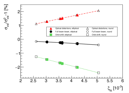
Figure 21: Dependence of the visible cross-section bias on the round-beam equivalent beam-beam parameter $\xi_{R}$, for optical distortions only (red), orbit shift only (green), and full beam-beam effect (black). The filled (open) markers tag the results of individual B*B simulations assuming upright elliptical (round) beams; the orbit-shift bias is calculated analytically using the elliptical-beam formula [6]. The curves show the round-beam estimates based on the parameterization of Eqs. (34)-(35). The points clustered around each $\xi_{R}$ value correspond to different settings of the $\Sigma^{0}_{y}$/$\Sigma^{0}_{x}$ aspect ratio.

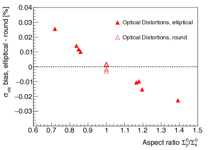
Figure 22: Aspect-ratio dependence of the difference in $\,\sigma_{\mathrm{vis}}$ bias associated with optical distortions, between the result of B*B elliptical-beam simulations, and the corresponding round-beam estimate based on the parameterization of Eqs. (34)-(35). The filled (open) markers tag the results of individual simulations assuming upright elliptical (round) beams. The points clustered around each value of the aspect ratio correspond to different $\xi_{R}$ settings. The horizontal dashed line corresponds to no difference in $\,\sigma_{\mathrm{vis}}$ bias between round and elliptical beams. The spread of the round-beam simulation results (open triangles) reflects the numerical accuracy of the subtracted parameterization.

4.5 Impact of non-zero crossing angle

In the presence of a significant crossing angle, the analysis becomes considerably more involved, and a full exposition thereof would exceed the scope of the present report. The discussion below is therefore focussed on assessing the beam-beam correction uncertainty associated with scans at zero nominal crossing angle, during which the actual, residual crossing angle does not exceed few tens of microradians: this covers most luminosity-calibration sessions at IP1 (ATLAS) and IP5 (CMS). The same treatment, albeit at the cost of a small additional uncertainty, remains applicable to scans at IP2 (ALICE) (and to some non-standard sessions at IPs 1 and 5) that involve nominal crossing angles $\theta_{c}$ in the 140–400 $\mu$rad range. At IP8 however, the LHCb requirement for an unambiguous separation, in the crossing plane, of beam-gas vertices from beam 1 and beam 2, leads to $\theta_{c}$ settings of up to 1100 $\mu$rad. Such large crossing angles would require simulation studies more extensive than can be reported here.

In the absence of any beam-beam interaction, the geometric factor $F$ defined in Eq. (11), and generalizations thereof [8, 10], provide an accurate description of the combined impact of a non-zero crossing angle and of a finite bunch length on the unperturbed apparent transverse beam size in the crossing plane, as well as of the beam-separation dependence of the unperturbed luminosity.

In the presence of the beam-beam interaction, the implications of a non-zero crossing-angle for the calculation of beam-beam biases fall in two conceptually distinct categories.

• Geometrical effects in the transverse plane that depend on the crossing angle and on the bunch length, such as modifications of the transverse beam-beam overlap and the calculation of the effective strength of the source field experienced by the particles in the witness beam, are adequately modeled [8] by the B*B package and well reproduced by COMBI simulations. B*B simulations, however, are intrinsically limited to four dimensions (horizontal and vertical positions and angles), since the longitudinal variables are “projected out” and the associated dynamics implicitly neglected.

• Longitudinal dynamics, such as synchrotron motion or beam–beam-induced transverse-shape variations along the bunch, can be modeled by COMBI using the 6D beam-beam strong-strong model [33]. This model divides particle distributions into slices along the length of each bunch. The kick experienced by each macroparticle in one beam is computed based on the statistical moments of the charge distributions in each slice of the opposing bunch; the computation is repeated for the macroparticles in the other beam.

In order to properly account for longitudinal effects and assess their importance, COMBI is chosen here to characterize the interplay of crossing-angle and beam-beam effects. This first study is exploratory in nature and restricted to the regime.

As predicted analytically [8, 44], the magnitude of the orbit shift extracted from COMBI simulations for a purely horizontal crossing angle of several hundred microradians, is found consistent with that computed using the Bassetti-Erskine formula with, as input:

• in the crossing (horizontal) plane, the effective convolved beam size given by $\Sigma_{x,eff}=F\times\Sigma_{x}$, where $F$ is the geometric factor defined in Eq. (11) and $\Sigma_{x}$ is the horizontal convolved beam size at zero crossing angle, given by Eq. (6);

• in the non-crossing (vertical) plane, the vertical convolved beam size $\Sigma_{y}$.

The dependence of the beam–beam-induced visible cross-section bias on the full crossing angle is illustrated in Fig. 23 for a beam-beam parameter setting typical of Run-2 scans. For the configurations shown in this figure, the geometric factor spans the range $1.0<F<1.09$. Since this factor impacts both $\,\sigma^{0}_{\mathrm{vis}}$ and $\,\sigma_{\mathrm{vis}}$ in an almost identical manner, it cancels in the crossing-angle dependence of the ratio $\,\sigma_{\mathrm{vis}}/\,\sigma^{0}_{\mathrm{vis}}$. The absolute value of the $\,\sigma_{\mathrm{vis}}$ bias increases with the angle, even though the “effective” beam-beam parameter in the crossing plane (i.e. that calculated from the effective transverse beam size) decreases. The difference between the horizontal- and vertical-crossing configurations is due to the difference between the $x$ and $y$ tunes. Also notable is the sensitivity to $\,\beta^{*}$: the crossing-angle dependence of the beam-beam bias is weaker for $\,\beta^{*}=24$ m than for $\,\beta^{*}=19$ m. The results are insensitive to the assumed value of the synchrotron tune, as well as to the chromaticity of the ring lattice (reducing the chromaticity to zero from its nominal setting of 15 units impacts the results by less than 0.01 %). This suggests that the effect is mostly geometrical in nature, as confirmed by the qualitative agreement of the COMBI results with those of a preliminary B*B study that covered a similar parameter space.

In practical terms, the impact of the crossing angle on the estimated beam-beam correction can be taken as the difference in visible cross-section bias between $\theta_{c}=0$ and the actual crossing-angle value. For a nominally zero crossing angle, the actual angle, as measured by the BPM system or by K-modulation in the final-triplet quadrupoles, is of the order of $10\,\mu\mathrm{rad}$: the associated shift in the beam-beam bias, as read off Fig. 23 at $\,\beta^{*}=19$ m, does not exceed 0.01%. For a nominal crossing angle around $150\,\mu\mathrm{rad}$, which is typical of ALICE sessions, neglecting the crossing angle would underestimate the beam-beam correction by less than 0.02%, a value small enough to be neglected. Crossing angles in excess of $500\,\mu$rad, however, induce still-to-be understood biases of 0.1% or more (Fig. 23), and may require further study.

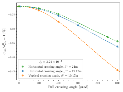
Figure 23: Crossing-angle dependence of the visible cross-section bias predicted by COMBI strong-strong, 6-dimensional simulations, for a horizontal (blue) and a vertical (orange) crossing angle at $\,\beta^{*}$ = 19.17 m, and for a horizontal crossing angle at $\,\beta^{*}$ = 24 m (green). The beam-beam parameter value at zero crossing angle is indicated in the legend. The beam energy, bunch intensity, normalized emittance, bunch length and tunes are fixed at, respectively, $E_{B}=6.5$ TeV, $n_{p}=0.783\times 10^{11}$ p/bunch, $\epsilon_{N}=2.95\,\mu$m$\cdot$rad, $\sigma_{z}=7.5$ cm, $\text{Q}_{x}=64.31$, $\text{Q}_{y}=59.32$, $\mathrm{Q_{s}}=0.0023$. The bunches are assumed to collide only at the IP where the scans are performed. The points are the results of the simulation; the lines are meant to guide the eye.

4.6 Impact of multiple interaction points

4.6.1 Motivation and methodology

All results presented in this paper so far assume that the beams collide at the scanning IP only, i.e. that they are fully separated, either transversely or longitudinally, at the other three IPs of the LHC. In practice however, this is often not the case: to make optimal use of beam time during luminosity-calibration scans at, say, the CMS IP, the experimental detectors at some or all of the other IPs typically collect collision data at fixed (most often zero) beam separation, thereby significantly affecting the unperturbed-tune spectra and therefore the magnitude of beam-beam induced biases.

For a given colliding-bunch pair at a given scanning IP, the number of non-scanning interaction points $N_{\mathrm{NSIP}}$ is defined as the average number of head-on collisions experienced, at interaction points other than the scanning IP, by the two members of the pair. The parameter $N_{\mathrm{NSIP}}$ ranges from zero when beams are fully separated at all but the scanning IP, to $N_{\mathrm{NSIP}}=3$ when both bunches in the pair collide at three other IPs; it can assume half-integer values when the two members of the pair experience different numbers of additional collisions.

Because IP1 (ATLAS) and IP5 (CMS) are separated by half a ring circumference, all bunches that collide in IP1 also collide in IP5, unless fully separated in the transverse plane at the non-scanning IP. Each member of such a colliding-bunch pair can optionally also collide in IP2 (ALICE) and/or IP8 (LHCb), both of which are located 1/8th of the ring away from IP1; however its collision “partner” at these IPs cannot be the same as that at IPs 1 and 5, because of the ring layout (Fig. 24). Injected-bunch patterns are optimized, on a fill-by-fill basis, to achieve the desired sharing of collisions (or absence thereof) among the four experimental detectors.

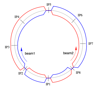
Figure 24: Schematic layout of the LHC beams and interaction points. Interaction points 1, 2, 5 and 8 house, respectively, the ATLAS, ALICE, CMS and LHCb experiments. (Figure reproduced from Ref. [22], © CERN)

The parameter $N_{\mathrm{NSIP}}$, therefore, depends on the scanning IP considered, and, for a given scanning IP, can vary along the bunch string in a manner that depends on the injected-bunch pattern. From 2010 to 2017, the most frequent configuration during $pp$ scans at the ATLAS and CMS IPs corresponded to $N_{\mathrm{NSIP}}=1$ at IPs 1 and 5, i.e. to bunches that collide in IP1 and IP5 only; from 2018 onwards, all four scanning IPs had to deal with multiple non-scanning IPs, for reasons of operational efficiency.

In order to characterize the impact of multiple collision points on beam-beam corrections to luminosity calibrations, COMBI was used to simulate scans at one IP (e.g. IP1), with additional head-on collision points optionally inserted at one or more other IPs (in this example IP5, IP2 and/or IP8). The bunch parameters are listed in Table 5. The beam transport between consecutive IPs is modeled by linear maps that reflect the nominal phase advance in the LHC rings during the Run-2  sessions at $\sqrt{s}=13$ TeV (Table 6), and head-on collisions are simulated at each non-scanning IP as described in Sec. 3.4. The unperturbed beams satisfied the assumptions listed in Sec. 4.1, except for the absence of additional collisions.

Parameter	Value
Beam energy $E_{B}$ [TeV]	6.5
Typical bunch population $n_{p}$ [$10^{11}$]	0.78
Bunches colliding	1
$\epsilon_{N}$ [$\mu$m-rad]	2.9
IP1,5: $\,\beta^{*}$ [m]	19.2
IP2/8: $\,\beta^{*}$ [m]	19.2 / 24.0
$\theta_{c}$ [$\mu$rad]	0
$\Sigma^{0}_{x}=\Sigma^{0}_{y}$ [$\mu$m]	128
Nominal tune settings $\text{Q}_{x}$/$\text{Q}_{y}$	64.31/59.32
Typical $\xi$ [per IP]	0.0032

Table 5: Beam conditions assumed for the multi-IP simulations described in Sec. 4.6. The crossing angle $\theta_{c}$ is set to 0 at all IPs so as to fully decouple the multi-IP study from potential longitudinal-dynamics effects.

Beam 1			Beam 2
From - to	$\mu_{\mathrm{x}}^{{\mathrm{B}}1}~{}[2\pi]$	$\mu_{\mathrm{y}}^{{\mathrm{B}}1}~{}[2\pi]$	From - to	$\mu_{\mathrm{x}}^{{\mathrm{B}}2}~{}[2\pi]$	$\mu_{\mathrm{y}}^{{\mathrm{B}}2}~{}[2\pi]$
IP1 - IP5	31.9757	29.6486	IP5 - IP1	31.9844	29.7613
IP5 - IP1	32.3343	29.6714	IP1 - IP5	32.3256	29.5587
IP1 - IP2	8.2960	7.6692	IP2 - IP1	8.2728	7.9577
IP2 - IP5	23.6797	21.9794	IP5 - IP2	23.7116	21.8036
IP5 - IP8	24.0891	21.3685	IP8 - IP5	23.8146	21.9544
IP8 - IP1	8.2452	8.3029	IP1 - IP8	8.5110	7.6042
Full turn	64.3100	59.3200	Full turn	64.3100	59.3200

Table 6: Horizontal ($\mu_{\mathrm{x}}$) and vertical ($\mu_{\mathrm{y}}$) betatron phase advance between consecutive collision points in the LHC Run-2  configuration for $pp$ collisions at $\sqrt{s}=13$ TeV. Beam 1 moves from the top to the bottom row, beam 2 from the bottom to the top row.

This Section is organized as follows. Multi-IP collisions increase the beam-beam tune spread, thereby shifting the means of the unperturbed-tune spectra to lower values (Sec. 4.6.2). They also affect the peak-rate and beam-size bias factors in a manner that depends on the phase advance between consecutive collision points around the rings, but that leaves the $\,\sigma_{\mathrm{vis}}$ bias almost totally insensitive to these phase-advance values. The analysis can be greatly simplified by an astute choice of the reference “no beam-beam” configuration (Sec. 4.6.3), up to a small residual ambiguity that depends on the phase advance between the non-scanning IP(s) and that where the scans are taking place (Sec. 4.6.4). This approach naturally leads to an effective parameterization of the impact of multi-IP collisions on beam-beam corrections to  calibrations (Sec. 4.6.5). Candidate beam-beam correction strategies in the presence of multi-IP collisions are summarized in Sec. 4.6.6.

4.6.2 Impact of multiple interaction points on the tune spectra

A comparison of simulated vertical-tune spectra for $N_{\mathrm{NSIP}}=0$ and $N_{\mathrm{NSIP}}=1$ is presented in Fig. 25. The single-IP beam-beam parameter $\xi$ is chosen to be typical of scans in $pp$ collisions. For beams colliding at the scanning IP only ($N_{\mathrm{NSIP}}=0$), two narrow peaks appear: one near the nominal tune ($\text{q}_{x}\approx 0.320$), and the other near $\text{q}_{x}-Y*\xi$, where $Y\approx 1.1$ is the Yokoya factor in the soft-Gaussian approximation [45]. These peaks correspond to, respectively, the so-called $\sigma$ and $\pi$ modes of coherent bunch oscillation. When beams collide in addition at one non-scanning IP ($N_{\mathrm{NSIP}}=1$), the peak of the $\sigma$ mode is unaffected, but the beam-beam tune spread roughly doubles and the $\pi$ mode is shifted further down, near $\text{q}_{x}-2Y*\xi$. In both cases, the mean tunes lie roughly half-way between the $\sigma$ and $\pi$ peaks, and therefore differ by roughly $-\xi/2$ between the two configurations. Adding a second non-scanning IP results in a further widening of the tune spread, to roughly three times that for $N_{\mathrm{NSIP}}=0$, and in a correspondingly larger downward shift of the mean tune.

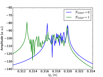
Figure 25: Vertical coherent-tune spectra in collisions simulated using COMBI, for head-on collisions at the scanning IP only ($N_{\mathrm{NSIP}}=0$, blue curve), and in the presence of head-on collisions at one additional IP ($N_{\mathrm{NSIP}}=1$, green curve). The beams satisfy the assumptions listed in Sec. 4.1, except for the absence of additional collisions. The beam-beam parameter $\xi$ is set to $3.24\times 10^{-3}$ per collision, and the tunes to their nominal value $(\text{Q}_{x},\text{Q}_{y})=(64.31,59.32)$

4.6.3 Comparison of reference “no beam-beam” configurations in the presence of one non-scanning IP

In Secs. 2, 3 and 4.1 to 4.5, it is implicitly assumed that the beams collide at the scanning IP only. The beam–beam-induced peak-rate, beam-size and luminosity-bias factors defined in Sec. 4.2.4 are all expressed with respect to an unambiguous reference configuration that corresponds to “no beam-beam anywhere”, in which the “nominal ” reference variables ($\sigma_{0}$, $\,\mu^{0}_{pk}$, $\Sigma^{0}_{x}$, $\Sigma^{0}_{y}$, $\mathcal{L}^{0}$, $\,\sigma^{0}_{\mathrm{vis}}$,…) are identified by a “0” index.

In the presence of collisions at non-scanning IPs, however, an ambiguity arises: should beam-beam-induced biases be referenced to a configuration in which the beam-beam interaction is switched off at every single IP, or to one in which the beam-beam interaction is switched off at the scanning IP only, but remains active at the non-scanning IPs (if any)?

Confronting this question requires a more precise nomenclature than that used so far:

• when the reference configuration is one in which the beam-beam interaction is switched off at all IPs, i.e. if  observables are corrected to “no beam-beam anywhere”, the corresponding reference variables carry a “0” index as before. In particular, the reference luminosity $\mathcal{L}_{\mathrm{no-bb}}$ at the scanning IP is equal to the nominal luminosity defined in Sec. 2.3.2 ($\mathcal{L}_{\mathrm{no-bb}}=\mathcal{L}^{0}$). This is referred to below as the “$\mathcal{L}^{0}$ normalization”;

• when the reference configuration is one in which  observables are corrected to “no beam-beam at the scanning IP only” even when the bunches considered also collide at one or more other IPs, the corresponding reference variables carry a “$u$” index instead. In particular, the reference luminosity $\mathcal{L}_{\mathrm{no-bb}}$ at the scanning IP is given by the unperturbed luminosity $\mathcal{L}^{u}$ ($\mathcal{L}_{\mathrm{no-bb}}$ = $\mathcal{L}^{u}$), i.e. that which would be measured at the scanning IP if the beam-beam interaction could be turned off at that IP only. This quantity is accessible only in simulations; its beam-separation dependence is in general notably different from that of $\mathcal{L}^{0}$. The same notation, and physical meaning, are applied to the other reference variables. This is referred to below as the “$\mathcal{L}^{u}$ normalization”;

• in the limiting case of collisions at the scanning IP only ($N_{\mathrm{NSIP}}=0$), $\mathcal{L}^{u}$ and $\mathcal{L}^{0}$ are one and the same, as are all the other reference variables: there is no difference between “nominal” and “unperturbed” quantities.

The beam-separation dependence of the $\mathcal{L}^{u}/\mathcal{L}^{0}$ ratio, during a vertical scan at IP1 and in the presence of head-on collisions at IP5, is presented in Fig. 26 (blue lozenges). Even though the unperturbed luminosity $\mathcal{L}^{u}$ is by definition unaffected by beam-beam effects at the scanning IP, it exhibits a monotonic increase with beam separation when compared to the reference luminosity $\mathcal{L}^{0}$. This seemingly counter-intuitive observation is explained by the fact that the horizontal axis in Fig. 26 is the nominal transverse beam size $\sigma^{0}$, not the actual beam size during the scan; equivalently, the actual relative separation, i.e. that normalized to the actual unperturbed beam size, differs from the nominal relative separation, which is normalized to the nominal beam size. The monotonic increase of the $\mathcal{L}^{u}/\mathcal{L}^{0}$ ratio therefore suggests that in this particular configuration, the collisions at IP5 result in an enlarged vertical convolved beam size at IP1 ($\Sigma^{u}_{y}>\Sigma^{0}_{y}$). This interpretation is confirmed by the evolution, during the scan, of the individual unperturbed single-beam sizes $\sigma^{u}_{yB}$ ($B=1,2$) that is illustrated in Fig. 27 (open lozenges): both are larger than $\sigma_{0}$, they remain constant as a function of the beam separation at the scanning IP, and their difference reflects the fact that the vertical phase-advance values from IP1 to IP5 differ significantly between the two beams (Table 6, top two rows).

Also shown in Fig. 26 is the luminosity-bias factor $[\mathcal{L}/\mathcal{L}^{0}]_{\mathrm{Full\,BB}}$ in the $\mathcal{L}^{0}$ normalization (red squares), that displays an $s$-like shape superposed on the monotonic beam-separation dependence of the $\mathcal{L}^{u}/\mathcal{L}^{0}$ curve. The ratio of these two curves:

$$[\mathcal{L}/\mathcal{L}^{0}]_{\mathrm{Full\,BB}}\,/\,(\mathcal{L}^{u}/\mathcal{L}^{0})=[\mathcal{L}/\mathcal{L}^{u}]_{\mathrm{Full\,BB}}$$

represents the luminosity-bias factor in the $\mathcal{L}^{u}$ normalization in the presence of one non-scanning IP ; it is displayed as filled green circles, and is highly reminiscent of the black curve in Fig. 9.

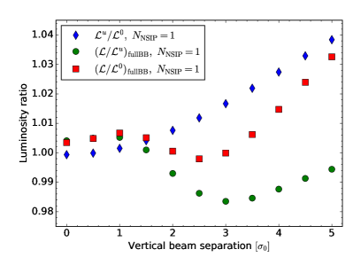
Figure 26: Beam-separation dependence, during a simulated vertical  scan in the Run-2 configuration with one non-scanning IP, of the luminosity-bias factors at the scanning IP associated with the unperturbed luminosity ($\mathcal{L}^{u}/\mathcal{L}^{0}$, blue lozenges), with the full beam-beam effect in the $\mathcal{L}^{0}$ normalization ($[\mathcal{L}/\mathcal{L}^{0}]_{\mathrm{Full\,BB}}$, red squares), and with the full beam-beam effect in the $\mathcal{L}^{u}$ normalization ($[\mathcal{L}/\mathcal{L}^{u}]_{\mathrm{Full\,BB}}$, filled green circles). The horizontal axis is the beam separation in units of the nominal transverse beam size $\sigma_{0}$.

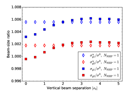
Figure 27: Beam-separation dependence, during a simulated vertical  scan, of the beam–size-bias factors at the scanning IP associated with the full beam-beam effect ($\sigma_{yB}/\sigma^{0}$, filled squares) and of the corresponding unperturbed quantities ($\sigma^{u}_{yB}/\sigma^{0}$, open lozenges), separately for B = beam 1 (blue) and B = beam 2 (red), using the $\mathcal{L}^{0}$ normalization and in the presence of collisions at one non-scanning IP ($N_{\mathrm{NSIP}}=1$). The horizontal axis is the beam separation in units of the nominal transverse beam size $\sigma_{0}$.

This same luminosity-bias factor that is presented in Fig. 26 for $N_{\mathrm{NSIP}}=1$, is compared in Fig. 28 to the equivalent quantity for $N_{\mathrm{NSIP}}=0$. Up to a small systematic difference that represents the impact of the additional head-on collisions that occur at the non-scanning IP, the two curves are essentially identical. This observation suggests that the beam-separation dependence of the beam–beam-induced orbit-shift and optical-distortion effects is encapsulated in that of $[\mathcal{L}/\mathcal{L}^{u}]_{\mathrm{Full\,BB}}$, even in the presence of collisions at the non-scanning IP(s). This interpretation is confirmed by comparing the separation dependence of the actual single-beam transverse RMS sizes $\sigma_{iB}$ ($i=x,y$; $B=1,2$) with, and without, additional collisions at the non-scanning IP. When $N_{\mathrm{NSIP}}=1$ (Fig. 27), $\sigma_{y1}>\sigma_{y2}$; these two quantities exhibit a very similar beam-separation dependence with respect to the corresponding unperturbed beam size $\sigma^{u}_{yB}$. A direct comparison of the $\sigma_{yB}/\sigma^{u}_{yB}$ ratio with and without a non-scanning IP (Fig. 29) shows that the two configurations result in an almost identical beam-separation dependence, the shape of which closely parallels that computed [4] in the linear approximation using MADX, once the qualitative impact of amplitude detuning is taken into account.

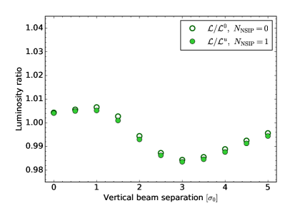
Figure 28: Beam-separation dependence, during a simulated vertical  scan, of the luminosity-bias factors at the scanning IP associated with the full beam-beam effect, for $N_{\mathrm{NSIP}}=0$ using the $\mathcal{L}^{0}$ normalization (open circles), and for $N_{\mathrm{NSIP}}=1$ using the $\mathcal{L}^{u}$ normalization (filled green circles). The horizontal axis is the beam separation in units of the nominal transverse beam size $\sigma_{0}$. The span of the vertical scale is identical to that of Fig. 26.

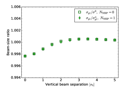
Figure 29: Beam-separation dependence, during a simulated vertical  scan, of the beam–size-bias factors at the scanning IP associated with the full beam-beam effect for $N_{\mathrm{NSIP}}=0$ using the $\mathcal{L}^{0}$ normalization ($\sigma_{y1}/\sigma^{0}$, open squares), and for $N_{\mathrm{NSIP}}=1$ and using the $\mathcal{L}^{u}$ normalization ($\sigma_{y1}/\sigma^{u}_{y1}$, filled green lozenges). For the sake of clarity, only beam-1 results are displayed; the beam-2 points would be indistinguishable. The horizontal axis is the beam separation in units of the nominal transverse beam size $\sigma_{0}$. The span of the vertical scale is identical to that of Fig. 27.

The contrast in beam-separation dependence between the nominal ($\mathcal{L}^{0}$) and the unperturbed ($\mathcal{L}^{u}$) luminosity-bias curves apparent in Fig. 26, and the “universality” of the $[\mathcal{L}/\mathcal{L}^{u}]$ luminosity-bias curves (Fig. 28), can be further characterized by comparing the separation dependence of the unperturbed luminosity $\mathcal{L}^{u}$, computed numerically as the overlap integral over the unperturbed macroparticle distributions, with that of its Gaussian-equivalent counterpart $\mathcal{L}^{u}_{\mathrm{Geq}}$. The latter is defined as:

$$\mathcal{L}^{u}_{\mathrm{Geq}}(\delta_{x})=\frac{1}{2\pi\Sigma^{u}_{x\mathrm{,Geq}}\Sigma^{u}_{x\mathrm{,Geq}}}\exp\left[-\frac{1}{2}\left(\frac{\delta_{x}}{\Sigma^{u}_{x\mathrm{,Geq}}}\right)^{2}\right]\,,$$

and similarly for $\mathcal{L}^{u}_{\mathrm{Geq}}(\delta_{y})$. It is calculated under the assumption that the unperturbed macroparticle distributions are Gaussian, and adequately described (for this particular purpose) by the transverse RMS single-beam sizes $\sigma^{u}_{iB}$ ($i=x,y$; $B=1,2$):

$$\Sigma^{u}_{i\mathrm{,Geq}}=\sqrt{(\sigma^{u}_{i1})^{2}+(\sigma^{u}_{i2})^{2}}\,.$$

The comparison between $\mathcal{L}^{u}$ and $\mathcal{L}^{u}_{\mathrm{Geq}}$ is presented in Fig. 30. During the vertical scan (filled symbols), the unperturbed luminosity (already shown in Fig. 26) and its Gaussian-equivalent counterpart are almost exactly equal, except at large separation ($\delta_{y}/\sigma^{0}>4$); both increase with separation relative to $\mathcal{L}^{0}$. The same occurs during the horizontal scan (open symbols), except that here both curves drop with increasing separation, because the horizontal phase advances are such that the dynamic-$\beta$ effect at IP5 translates into smaller horizontal beam sizes at IP1. As already documented [4] in the linear approximation, the dynamic-$\beta$ effect at the non-scanning IP(s) propagates to the scanning IP, resulting in either larger or smaller unperturbed transverse beam-sizes depending on the phase advance.

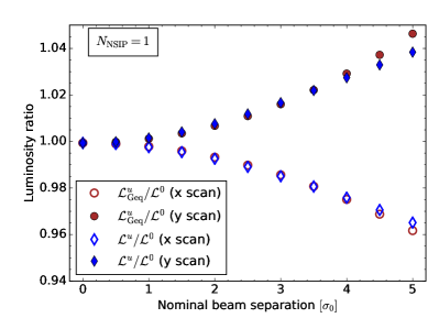
Figure 30: Beam-separation dependence, during  scans simulated in the Run-2 configuration with one non-scanning IP, of the luminosity-bias factors at the scanning IP associated with the unperturbed luminosity ($\mathcal{L}^{u}/\mathcal{L}^{0}$, lozenges), and with the Gaussian-equivalent unperturbed luminosity ($\mathcal{L}^{u}_{\mathrm{Geq}}/\mathcal{L}^{0}$, circles). The horizontal axis is the beam separation in units of the nominal transverse beam size $\sigma_{0}$. The filled (open) symbols corresponds to a vertical (horizontal) scan.

The fundamental observable of the van der Meer method is the beam-separation dependence of the measured interaction rate. Intuitively therefore, one can argue that a separation-independent change in unperturbed transverse beam size at the scanning IP (Fig. 27, open symbols) should not bias the $\,\sigma_{\mathrm{vis}}$ measurement, provided the shift in unperturbed tunes is properly accounted for. The same reasoning is offered in Ref. [4], where the argument is more straightforward: in the linear approximation (Sec. 3.1), additional collisions are tantamount to inserting a quadrupole-like perturbation at the non-scanning IP(s), that in turn results in a small tune shift accompanied by a $\beta$-beating wave around each ring. In the more general case treated here, the excellent agreement between $\mathcal{L}^{u}$ and $\mathcal{L}^{u}_{\mathrm{Geq}}$ over most of the scanning range (Fig. 30) indicates that the dominant effect is that of a beam- and plane-dependent shift of the effective $\,\beta^{*}$ value, and of the corresponding unperturbed RMS single-beam sizes. Non-Gaussian tails associated with the non-linearity of the beam-beam force at the non-scanning IP(s) have but a very minor impact on the unperturbed transverse-density distributions at the scanning IP.

As a first illustration of the magnitude of multi-IP effects and of the quantitative impact, on beam-beam corrections, of the difference between the green circles and the red squares in Fig. 26, Table 7 compares the separation-integrated FoMs (Sec. 4.2.4) extracted from a simulated -scan pair at IP1, with and without additional head-on collisions at IP5.

• In the $\mathcal{L}^{u}$ normalization, and as expected from Fig. 28, the hierarchy of the FoMs is very similar with ($N_{\mathrm{NSIP}}=1$) and without ($N_{\mathrm{NSIP}}=0$) collisions at the non-scanning IP. The beam-beam bias is systematically more negative for $N_{\mathrm{NSIP}}=1$: this is qualitatively consistent with the combination of a decrease of the mean unperturbed tunes (Sec. 4.6.2), and of the tune-dependence of the luminosity-bias curves (Fig. 13). As a result, the magnitude of the overall beam-beam bias on $\,\sigma_{\mathrm{vis}}$ (row 7, columns 3 and 4) increases substantially in the presence of a non-scanning IP.

• For $N_{\mathrm{NSIP}}=1$, the hierarchy of the FoMs is very different in the $\mathcal{L}^{0}$ and $\mathcal{L}^{u}$ normalizations, because the dynamic-$\beta$ effect at the non-scanning IP has a significant impact on the transverse unperturbed beam sizes at the scanning IP (Fig. 27). The fact that the $\Sigma_{x}$ ($\Sigma_{y}$) bias is more negative (positive) in the $\mathcal{L}^{0}$ normalization reflects the fact that the unperturbed horizontal (vertical) beam size at the scanning IP is smaller (larger) than its nominal value (Fig. 30).

• In contrast, the $\,\sigma_{\mathrm{vis}}$-bias values for $N_{\mathrm{NSIP}}=1$ agree to better than 0.005% between the $\mathcal{L}^{0}$ and $\mathcal{L}^{u}$ normalizations, indicating that in practice, the two normalizations yield equivalent beam-beam corrections. This can be understood by examining the bottom half of Table 7, that summarizes the impact of collisions at IP5 on the unperturbed scan variables at IP1: $\Sigma^{u}_{x}$ decreases, $\Sigma^{u}_{y}$ increases by a little more, resulting in a small decrease of the unperturbed peak interaction rate $\mu^{u}_{pk}$; the net change in $\,\sigma_{\mathrm{vis}}$ is at the 0.004% level. Physically, this expresses the fact that the changes in the unperturbed transverse convolved beam sizes and the unperturbed head-on luminosity are correlated such that the visible-cross-section remains invariant, at least in the configuration simulated here.

	$N_{\mathrm{NSIP}}=1$		$N_{\mathrm{NSIP}}=0$
	Normalization:
FoM	$\mathcal{L}_{\mathrm{no-bb}}$ =		$\mathcal{L}_{\mathrm{no-bb}}$ = $\mathcal{L}^{0}$
	$\mathcal{L}^{0}$	$\mathcal{L}^{u}$	($\mathcal{L}^{u}$ = $\mathcal{L}^{0}$)
Beam-beam bias on measured scan variables [%]
$\mu_{pk}/\mu^{\mathrm{n}o-bb}_{pk}-1$	0.346	0.410	0.431
$\Sigma_{x}/\Sigma^{\mathrm{n}o-bb}_{x}-1$	-0.784	-0.454	-0.405
$\Sigma_{y}/\Sigma^{\mathrm{n}o-bb}_{y}-1$	0.076	-0.323	-0.239
$\sigma_{vis}/\sigma^{\mathrm{n}o-bb}_{vis}-1$	-0.365	-0.369	-0.215
Beam-beam bias on unperturbed scan variables [%]
$\mu^{u}_{pk}/\mu^{\mathrm{n}o-bb}_{pk}-1$	-0.064	-	0
$\Sigma^{u}_{x}/\Sigma^{\mathrm{n}o-bb}_{x}-1$	-0.331	-	0
$\Sigma^{u}_{y}/\Sigma^{\mathrm{n}o-bb}_{y}-1$	0.401	-	0
$\sigma^{u}_{vis}/\sigma^{\mathrm{n}o-bb}_{vis}-1$	0.004	-	0

Table 7: Fractional peak-rate, beam-size and $\,\sigma_{\mathrm{vis}}$ beam–beam-induced bias on measured (rows 3-7) and unperturbed (rows 8-12) scan variables, for simulated scans at IP1, with (columns 2-3) and without (column 4) head-on collisions at IP5, using the nominal bunch parameters shown in Table 5 and the phase-advance settings listed in Table 6.

4.6.4 Sensitivity of beam-beam corrections to the phase advance between IPs

The results presented in the preceding paragraphs indicate that even though the separation dependence of the luminosity-bias factors are very different in the $\mathcal{L}^{0}$ and $\mathcal{L}^{u}$ normalizations (Fig. 26), these two reference configurations appear to yield almost identical beam-beam corrections to $\,\sigma_{\mathrm{vis}}$ (Table 7). What remains to be quantified is how robust this conclusion is against large variations in the assumed phase advance between consecutive IPs, as well as in the presence of more than one non-scanning IP.

The study reported in Sec. 4.6.3 assumes the phase-advance values between IP1 and IP5 that are listed in the top two rows of Table 6; these correspond to one point in four-dimensional phase-advance space ($\mu_{x}^{\mathrm{B}1},\mu_{y}^{\mathrm{B}1},\mu_{x}^{\mathrm{B}2},\mu_{y}^{\mathrm{B}2}$). To address the first question above, the analysis detailed in Sec. 4.6.3 was repeated while varying the horizontal and vertical phase advance between IP1 and IP5 over most of the $[0,2\pi]$ range, while keeping the nominal tunes constant; in order to keep the parameter space manageable, the B1 and B2 phase-advance values were in addition constrained to be the same, separately in the horizontal and the vertical plane ($\mu_{x}^{\mathrm{B}1}=\mu_{x}^{\mathrm{B}2}=\mu_{x}$, $\mu_{y}^{\mathrm{B}1}=\mu_{y}^{\mathrm{B}2}=\mu_{y}$). scans were simulated at IP1 over a grid in ($\mu_{x},\mu_{y}$) space, with the bunches colliding head-on at IP5, and using the bunch parameters listed in Table 5.

Inspection of the simulated tune spectra reveals that their detailed shape depends on the phase advance between IPs; the same applies to the transverse luminosity distributions. The interpretation is that particles at different amplitudes are subject to different combinations of beam-beam kicks at the scanning and the non-scanning IP, that depend on the phase advance between the two. Beam–beam-induced bunch-shape distortions at the non-scanning IP(s) propagate around the ring in a manner that depends on that phase advance, thereby making the detailed shape of the $\mathcal{L}^{u}$ distribution at the scanning IP phase–advance-dependent.

At each point in the ($\mu_{x},\mu_{y}$) space, the luminosity-bias curves and the corresponding separation-integrated FoMs were computed in both the $\mathcal{L}^{0}$ and the $\mathcal{L}^{u}$ normalization. The beam–beam-induced $\,\sigma_{\mathrm{vis}}$ bias, or equivalently the magnitude of the overall beam-beam correction to the -based absolute luminosity scale, was found to depend slightly on the choice of the reference “no beam-beam” configuration, i.e. on whether the beam-beam correction is calculated in the $\mathcal{L}^{0}$ or in the $\mathcal{L}^{u}$ normalization. The difference is phase-advance dependent, and exhibits a clear periodic structure (Fig. 31); a periodic structure is also observed in such two-dimensional maps of the luminosity-bias factor (not shown), with different patterns for $[\mathcal{L}/\mathcal{L}^{0}]$ and $[\mathcal{L}/\mathcal{L}^{u}]$. These periodicities have been shown not to be of statistical or numerical origin. The interplay between beam-beam effects at different IPs, and its sensitivity to the phase advance between IPs, was already observed at LEP-II, where it could strongly affect the instantaneous-luminosity balance between the four experimental detectors [46]. One tentative interpretation here is cross-talk between collision points: beam-beam kicks at one IP propagate to the other IP(s) in a phase-dependent manner, thereby modifying very slightly the corresponding density distributions as well as the associated beam-beam distortions. These perturbations then propagate back to the original IP, resulting in a small modulation of the $\,\sigma_{\mathrm{vis}}$ bias around the central value controlled by the unperturbed tunes. This and other potential explanations remain under study.

Fortunately, these subtle effects have only a minor impact on beam-beam corrections to calibrations. The largest amplitude of the $\mathcal{L}^{0}$-$\mathcal{L}^{u}$ discrepancy over the entire plane amounts to 0.06% of $\,\sigma_{\mathrm{vis}}$, which is smaller than, or at most comparable to, the absolute accuracy of the B*B or COMBI simulations. The reason why in Table 7 the $\mathcal{L}^{0}$ and $\mathcal{L}^{u}$ normalizations yield essentially identical results, is that the Run-2 phase-advance between IP1 and IP5 happens to lie in a region of the $\mu_{x}-\mu_{y}$ plane where the inconsistency is the smallest. In this case therefore, and for bunches that collide only in these two IPs, the difference in $\,\sigma_{\mathrm{vis}}$ bias between the $\mathcal{L}^{0}$ and $\mathcal{L}^{u}$ normalizations is negligible.

To assess the impact of more than one non-scanning IP, the above phase scans were repeated for collision patterns with up to three non-scanning IPs. To deal with the increased dimensionality of the problem, the fractional phase advance from IP1 to IP5 was fixed to $\Delta\mu_{x}=\Delta\mu_{y}=0.405$, a choice that in in Fig. 31 corresponds to the largest absolute difference in $\,\sigma_{\mathrm{vis}}$ bias between the $\mathcal{L}^{u}$ and $\mathcal{L}^{0}$ normalizations. With that constraint, and with the overall tunes and the IP5-IP8 phase advances fixed at their nominal values, the horizontal and vertical fractional phase-advance values from IP1 to IP2 were scanned over the range $[0,2\pi]$. The study was then repeated with the roles of IP2 and IP8 interchanged. In all these configurations, the difference in $\,\sigma_{\mathrm{vis}}$ bias between the $\mathcal{L}^{u}$ and $\mathcal{L}^{0}$ normalizations displays the same periodic pattern as that in Fig. 31, and the largest absolute difference in $\,\sigma_{\mathrm{vis}}$ bias between the two reference configurations does not exceed 0.15% (for $\xi=0.006$). While strictly speaking, the ensemble of these scans does not constitute an exhaustive sampling of the 12-dimensional phase-advance space (2 beams $\times$ 2 planes $\times$ 3 IP combinations), it suggests that the largest possible disagreement between the $\mathcal{L}^{0}$ and $\mathcal{L}^{u}$ normalizations amounts to 0.1-0.2% of $\,\sigma_{\mathrm{vis}}$ when considering the full parameter space. Since the phase advance between LHC IPs can be measured to a few degrees ($\sim 0.015\times 2\pi$) per beam and per plane, the “operating point” in phase-advance space is known to very good precision. In some cases therefore, the ambiguity on the $\,\sigma_{\mathrm{vis}}$ bias associated with the choice of reference configuration can be significantly reduced, as already demonstrated for bunches that collide in IP1 and IP5 only.

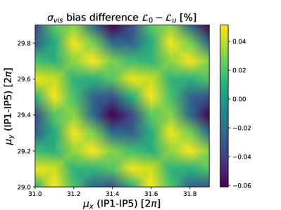
Figure 31: Phase-advance dependence of the difference, between the $\mathcal{L}^{0}$ and the $\mathcal{L}^{u}$ normalization, of the beam-beam induced $\,\sigma_{\mathrm{vis}}$ bias. The horizontal and vertical axes represent the betatron phase advance between IP1 and IP5, here assumed to be the same for B1 and B2. The color scale quantifies the fractional inconsistency in $\,\sigma_{\mathrm{vis}}$ bias between the two reference configurations; it ranges from $-0.06$ to $+0.05$% of $\,\sigma_{\mathrm{vis}}$.

4.6.5 Parameterization of multi-IP effects

To gain further insight into multi-IP effects and account, in a pragmatic fashion, for their impact on beam-beam corrections to luminosity calibrations, COMBI was used to simulate scans over the full range of beam-beam parameter values typical of sessions at $\sqrt{s}=13$ TeV, using the Run-2 phase-advance settings (Table 6), both without ($N_{\mathrm{NSIP}}=0$) and with ($1\leq N_{\mathrm{NSIP}}\leq 3$) head-on collisions at one or more non-scanning IP(s).

The results are summarized in Fig. 32 for three representative values of the single-IP beam-beam parameter $\xi$, using the $\mathcal{L}^{u}$ normalization. Since both the orbit-shift and the optical-distortion bias are sensitive to the unperturbed-tune values (Sec. 4.2.2), the overall beam-beam bias on the visible cross-section associated with a given value of $\xi$ is significantly affected by collisions at non-scanning IPs. Taking as an example the case of $\xi=6\times 10^{-3}$, the $\,\sigma_{\mathrm{vis}}$ bias when colliding only at the scanning IP amounts to $-0.55$% (orange circle). It grows to $-1.0$% for one non-scanning IP (pale-brown lozenge), to $-1.3$% for two non-scanning IPs (medium-brown lozenge), and to a little over $-1.5$% for the worst case of $N_{\mathrm{NSIP}}=3$ (darkest-brown lozenge). As $N_{\mathrm{NSIP}}$ increases by one unit, both the horizontal and the vertical mean unperturbed tune decrease by approximately $\xi/2$; as a consequence, the luminosity-bias curves shift downwards (Figs. 12, 13) and the $\,\sigma_{\mathrm{vis}}$ bias becomes accordingly more negative. The impact of this “multi-IP tune shift” is comparable in magnitude to the $\,\sigma_{\mathrm{vis}}$ bias for $N_{\mathrm{NSIP}}=0$; it varies from one bunch pair to another in a manner that depends on the single-bunch parameters and on the value of $N_{\mathrm{NSIP}}$ associated with each-colliding bunch pair at the IP where the scans are taking place. Fortunately however, this effect lends itself to a simple parameterization.

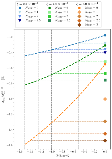
Figure 32: Horizontal lines, and markers at $\Delta\text{Q}_{\mathrm{mIP}}=0$: visible cross-section bias in the $\mathcal{L}^{u}$ normalization, associated with scans at IP1, for bunch pairs that in addition collide head-on at a fixed number of non-scanning IPs, and with the tunes set to their nominal value. The three sampled values of the single-IP beam-beam parameter $\xi$ are identified by the blue triangles ($\xi=2.7\times 10^{-3}$), green squares ($\xi=4.0\times 10^{-3}$) and brown lozenges ($\xi=6.0\times 10^{-3}$). For a given value of $\xi$, the lighter, medium and darker colors correspond to additional collisions at $N_{\mathrm{NSIP}}=1$, 2, 2.5 and 3 non-scanning IPs respectively (see text). Inclined curves and circular markers: visible cross-section bias associated with scans at IP1 with beams fully separated at all other IPs ($N_{\mathrm{NSIP}}=0$), as a function of the multi-IP equivalent mean tune shift $\Delta\text{Q}_{\mathrm{mIP}}$ expressed in units of $\xi$. The circular markers at $\Delta\text{Q}_{\mathrm{mIP}}/\xi=0$ show the value of the $\,\sigma_{\mathrm{vis}}$ bias corresponding to beams colliding only at the scanning IP, with the unperturbed tunes set to their nominal value. The vertical dashed lines correspond, from right to left, to $\Delta\text{Q}_{\mathrm{mIP}}/\xi=-0.5$, $-1.0$, $-1.25$ and $-1.5$, and approximately correspond to the values of the effective tune shift $\Delta\text{Q}_{\mathrm{mIP}}$ where an inclined curve associated with a given value of $\xi$ intersects the corresponding horizontal lines.

The diagonal curves in Fig. 32 display the visible cross-section bias for scans simulated at IP1 in the absence of collisions at any non-scanning IP, but with both the horizontal and the vertical unperturbed tunes shifted by a quantity $\Delta\text{Q}_{\mathrm{mIP}}$ that scales with $\xi$. For a given value of $\xi$, the intersections of the corresponding diagonal curve (orange in the example above) with the horizontal lines of the same hue corresponding to $N_{\mathrm{NSIP}}=1,2,...$, determine the magnitude of the multi-IP equivalent tune shift $\Delta\text{Q}_{\mathrm{mIP}}$ that needs to be applied simultaneously to the unperturbed horizontal and vertical tunes input to the COMBI simulation to mimic the effect of collisions at non-scanning IPs. The corresponding values of $\Delta\text{Q}_{\mathrm{mIP}}/\xi$ are indicated by the vertical dashed lines in the figure.

A more telling representation of the same results is offered in Fig. 33, which displays the multi-IP equivalent tune shift as a function of the number of non-scanning IPs. The results are consistent with a linear dependence that differs only slightly from the naive scaling law

$$\Delta\text{Q}_{\mathrm{mIP}}=-0.5\,\xi N_{\mathrm{NSIP}}=-p_{1}\,\xi N_{\mathrm{NSIP}}$$ (41)

inspired by the qualitative evolution of the tune spectra. The purely empirical, two-parameter linear fit represented by the purple solid line:

$$\Delta\text{Q}_{\mathrm{mIP}}=p_{0}-p_{1}\,\xi\,N_{\mathrm{NSIP}}$$

provides a slightly better parameterization than Eq. (41), and appears accurate at the level of $\Delta\text{Q}_{\mathrm{mIP}}\sim\pm 0.05\,\xi$.

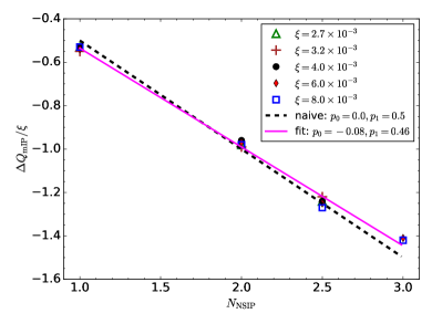
Figure 33: Dependence of the normalized multi-IP equivalent tune shift $\Delta\text{Q}_{\mathrm{mIP}}/\xi$ on the number of non-scanning IPs, for several values of the single-IP beam-beam parameter $\xi$. The scanning IP is set to IP1, and the $\,\sigma_{\mathrm{vis}}$ bias is calculated using the $\mathcal{L}^{u}$ normalization. The solid magenta line represents a two-parameter linear fit to the points; the black dashed line represents a naive parameterization of the form $\Delta\text{Q}_{\mathrm{mIP}}/\xi=-0.5\times N_{\mathrm{NSIP}}$.

Figure 33 demonstrates that for a given scanning IP and for all values of $\xi$, the normalized multi-IP equivalent tune shift scales linearly with the number of non-scanning IPs. To what extent this scaling is “universal”, i.e. how strongly it depends on the choice of the IP where the scans are taking place, is addressed by Fig. 34. Irrespective of the scanning IP considered, the overall dependence of the $\,\sigma_{\mathrm{vis}}$ bias on the number of scanning IPs is reasonably well represented by the naive scaling law of Eq. (41), demonstrating that the dominant effect is the downward shift of the mean unperturbed tunes. There are, however, significant differences between marker families, most notably between the red crosses (IP5) and the cyan squares (IP8): these reflect the variety of phase-advance patterns between the scanning IP and the other collision points. Similarly, within a given family, there exist several bunch pairings between B1 and B2 that yield the same number of additional collisions, but that correspond to different phase-advance configurations. When IP5 is the scanning IP, for instance, the configuration $N_{\mathrm{NSIP}}=2$ can be achieved with additional collisions at IP1 and at either IP2 or IP8; these two cases can therefore yield slightly different $\,\sigma_{\mathrm{vis}}$ biases. To minimize modeling errors, therefore, it is advisable that scaling parameterizations such as that illustrated by Fig. 33 be developed for each scanning IP separately, preferably taking into account the actual collision pattern experienced by each bunch that collides at the scanning IP under consideration.

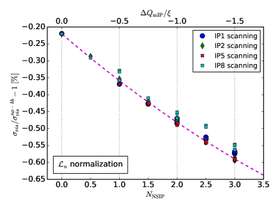
Figure 34: Visible cross-section bias in the $\mathcal{L}^{u}$ normalization as a function of the number of non-scanning IPs (lower horizontal axis), for the four possible choices of scanning IP. The curve represents the dependence of the $\,\sigma_{\mathrm{vis}}$ bias in the $N_{\mathrm{NSIP}}=0$ case, but with the horizontal and vertical unperturbed tunes shifted downwards by $\Delta\text{Q}_{\mathrm{mIP}}/\xi=-0.5\times N_{\mathrm{NSIP}}$ (upper horizontal axis). For a given scanning IP, there exist several B1-B2 bunch-collision patterns that yield the same value of $N_{\mathrm{NSIP}}$. The beam-beam parameter and phase-advance values are listed in Tables  5 and 6 respectively.

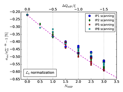
Figure 35: Visible cross-section bias in the $\mathcal{L}^{0}$ normalization as a function of the number of non-scanning IPs, for the four possible choices of scanning IP. The results are extracted from the same simulations as those in Fig. 34; only the reference configuration differs. The curve, the axis scales and the legend are identical.

Pursuing the same strategy in the $\mathcal{L}^{0}$ normalization meets with limited success (Fig. 35): for a given value of $N_{\mathrm{NSIP}}$, the spread across different collision patterns is noticeably larger than in the $\mathcal{L}^{u}$ normalization, even when restricted to one given scanning IP. This observation reflects the same underlying physics as the periodic structure in Fig. 31; its implications are addressed below.

4.6.6 Beam-beam correction strategies in the presence of multi-IP collisions

In summary, collisions at non-scanning IPs manifest themselves in two main ways. The widening of the tune spectra and the resulting downward shift of the mean unperturbed tunes (Sec. 4.6.2) significantly increase the beam–beam-induced bias on the absolute luminosity scale (Fig. 34), mainly because of the reduced amplitude of the optical-distortion bias (Sec. 4.2.2). This tune shift is accompanied by a beam- and plane-dependent $\beta$-beating wave around each ring [4], that translates into a sub-percent rescaling of the unperturbed transverse single-beam sizes at the scanning IP (Fig. 27). The latter causes significant distortions of the luminosity-bias curves when using the $\mathcal{L}^{0}$ normalization (Fig. 26), that depend strongly on the phase advance between consecutive collision points.

The shift in unperturbed tunes (Sec. 4.6.2) has, by far, the dominant impact on beam-beam corrections to calibrations. It can be accounted for by simulating collisions simultaneously at all relevant IPs, with the input tunes set to their nominal value, and by correcting the luminosity-scan curves to “no beam-beam anywhere”. This $\mathcal{L}^{0}$ normalization is the approach adopted in Ref. [8]. The alternative is to use the $\mathcal{L}^{u}$ normalization. It is inspired by the fact that the fundamental observable of the method is the beam-separation dependence of the measured interaction rate. What should matter, therefore, is the variation of the beam-beam force during the scan: underlying, separation-independent modifications of the unperturbed transverse-density distributions are expected not to affect the visible cross-section. In the $\mathcal{L}^{u}$ approach, the luminosity-scan curves extracted from the same multi-IP simulation as above are corrected to “no beam-beam at the scanning IP only” (Sec. 4.6.3); the resulting luminosity-bias functions become much less sensitive to the presence of non-scanning IPs (Fig. 28).

The $\mathcal{L}^{0}$ and $\mathcal{L}^{u}$ normalizations yield beam-beam corrections that, depending on the phase advance between consecutive IPs, either are indistinguishable (Table 7), or in the worst case differ by at most 0.1-0.2% of $\,\sigma_{\mathrm{vis}}$ (Sec. 4.6.4). These observations demonstrate that no phase-advance configuration exists in which beam-beam induced $\beta$-beating would significantly reduce the beam-beam bias on $\,\sigma_{\mathrm{vis}}$.

The results of the full multi-IP simulations can be very closely approximated by those of the much faster single-IP simulation, with as input the same value of the beam-beam parameter $\xi$, but with the unperturbed tunes shifted downwards by an amount $\Delta\text{Q}_{\mathrm{mIP}}$ that in the $\mathcal{L}^{u}$ normalization and for a given scanning IP, scales with $\xi$ and depends linearly on $N_{\mathrm{NSIP}}$ (Fig. 33). The scaling parameters are not fully universal, in the sense that they depend slightly on the choice of scanning IP (Fig. 34), or more fundamentally on the phase advance between the scanning and non-scanning IPs.

Clarifying the origin of the periodic structures in Fig. 31, and explaining why beam-beam corrections appear less sensitive to phase-advance effects in the $\mathcal{L}^{u}$ (Fig. 34) than in the $\mathcal{L}^{0}$ (Fig. 35) normalization, are topics of active study that lie beyond the scope of the present report. An ambiguity remains, therefore, as to which of the two reference “no beam-beam” configurations (i.e. which of the $\mathcal{L}^{0}$ or the $\mathcal{L}^{u}$ normalization) provides the most accurate beam-beam correction in absolute terms. Until this can be resolved, it seems prudent to keep the question open and to cover the difference by assigning a phase–dependence-related systematic uncertainty to the absolute magnitude of the beam-beam corrections.

On the practical side, the $\mathcal{L}^{u}$ normalization offers several advantages. First, by reducing the multi-IP problem to that of a single collision point, it greatly simplifies the interpretation of simulation results and the estimate of systematic uncertainties. The $\mathcal{L}^{u}$ approach also automatically accounts for the static (in the sense of separation-independent) change in unperturbed beam size associated with the dynamic-$\beta$ effect at the non-scanning IPs, preventing it from blurring the distinction between orbit-shift and optical-distortion corrections. Finally, combining the parameterization of single-IP beam-beam biases offered in Sec. 4.2.3 with the scaling prescriptions of Sec. 4.6.5 provides a beam–beam-correction procedure that is straightforward to implement, requires no or little investment by individual users in complex, CPU-intensive simulations, and is in many cases sufficient to calculate absolute bunch-by-bunch corrections to calibrations, or to estimate systematic uncertainties. This is particularly valuable when dealing with five to ten -scan pairs that involve up to 150 colliding bunches with different populations and emittances, arranged in multiple collision patterns that each require a different multi-IP correction [40]: the computing overhead that would be associated with simulating each of those configurations in detail is considerable.

The scaling prescriptions offered in Sec. 4.6.5 in the $\mathcal{L}^{u}$ normalization account for collisions at non-scanning IPs to better than 0.1-0.2% on $\,\sigma_{\mathrm{vis}}$. It should be stressed, however, that these simple-minded models reproduce only the $\,\sigma_{\mathrm{vis}}$ bias extracted from the multi-IP simulation (to an accuracy limited by the phase–advance-dependent inconsistency between the $\mathcal{L}^{0}$ and $\mathcal{L}^{u}$ normalizations), but that they are not meant to reproduce the corresponding tune spectra. An additional limitation is that they assume that collisions at non-scanning IPs occur with zero transverse separation, and with zero crossing angle. These ad hoc recipes are therefore no substitute for full-fledged simulations that account in detail for every distinct multi-IP collision pattern, separately for each scanning IP. For many purposes, however, these simple scaling laws appear sufficiently accurate to cover most beam conditions encountered during Run-2 sessions at the LHC. The potential interplay between multi-IP effects and scans in the presence of a large crossing angle, however, may require a dedicated study.

4.7 Impact of beam-beam asymmetry

The results presented so far in this chapter, with the exception of those in Sec. 4.4, assume beams that are round in the transverse plane ($\beta^{*}_{xB}=\beta^{*}_{yB}=\beta^{*}_{B}$ and $\sigma_{xB}=\sigma_{yB}=\sigma_{B}$, where $B=1,2$). In such a case, the distinction between horizontal and vertical beam-beam parameters disappears, and the beam-beam parameter of beam 2, defined in Eq. (12), simplifies to

$$\xi_{2}=\frac{n_{1}\,r_{0}\,\beta^{*}_{2}}{4\pi\,\gamma_{2}\,\sigma_{1}^{2}},$$ (42)

where $\sigma_{1}$ is the transverse RMS size of beam 1. The same formula, mutatis mutandis, is used to define $\xi_{1}$.

The parameterization described in Sec. 4.2, and the results derived therefrom, further assume that the beam-beam forces are exactly balanced between the two beams, i.e. that $\xi_{1}=\xi_{2}=\xi_{R}$ (Eq. (28)). Beam-beam asymmetry occurs when this assumption is violated, i.e. when $\xi_{1}\neq\xi_{2}$, which can arise under three different scenarios (Sec. 4.7.1). Even though a parametric approach can provide physically intuitive insight (Sec. 4.7.2), dedicated simulations are required to quantify the impact of such asymmetries on the accuracy of the beam-beam correction procedure (Sec. 4.7.3).

4.7.1 Beam-beam asymmetry scenarios

Consider first the case of a bunch-population asymmetry ($n_{1}\neq n_{2}$, with $\beta^{*}_{1}=\beta^{*}_{2}$ and $\sigma_{1}=\sigma_{2}$), which can be simulated in B*B by assigning different populations to the source beam and to the witness beam. Since the source beam in B*B remains unaffected by the beam-beam interaction, and since the two beams are subject to different beam-beam parameters, the simulation must be run twice, first with $n_{1}$ and $n_{2}$ assigned to, respectively, the source and the witness beam, and then with the inverse assignment. The predicted luminosity-bias curves, and the corresponding corrections to the FoMs, are then given by adding the two sets of results, implicitly assuming that strong-strong effects do not play a significant role even in the presence of a large bunch-population asymmetry (at least in the regime). This procedure was validated by confronting the B*B results with those from COMBI for several asymmetric configurations: even in the worst case considered ($n_{2}/n_{1}=2$, $\xi_{1}=5.30\times 10^{-3}$, $\xi_{2}=2.65\times 10^{-3}$), the beam-beam corrections calculated by the two packages agreed to better than one part in 1600.

The B*B and COMBI results above are accurately reproduced by the parameterization detailed in Sec. 4.2.3, with as input the beam-averaged beam-beam parameter:

$$\langle\xi\rangle=\frac{\xi_{1}+\xi_{2}}{2}~{}.$$ (43)

This is a consequence of the fact that the $\xi$-dependence of the FoMs is close enough to linear (Figs. 14–16) for the averaging of the FoM values at two different $\xi$ settings to be tantamount to computing the FoM once, with $\langle\xi\rangle$ as input.

The second scenario is that of a $\beta$-function asymmetry ($\beta^{*}_{1}\neq\beta^{*}_{2}$, with $n_{1}=n_{2}$ and $\sigma_{1}=\sigma_{2}$). This case is equivalent to that of the bunch-population asymmetry above, since only the product $n_{k}\beta^{*}_{l}$ ($k,l=1,2$ with $l\neq k$) plays a role in Eq. (42). The bunch population $n_{k}$ of beam $k$ controls the scale of the beam-beam force beam $k$ exerts on beam $l$, while $\beta^{*}_{l}$ determines how sensitive beam $l$ is to this force.

In contrast to the above two scenarios, which involve only scale effects, a beam-size or emittance asymmetry ($\sigma_{1}\neq\sigma_{2}$, with $n_{1}=n_{2}=n$ and $\beta^{*}_{1}=\beta^{*}_{2}=\,\beta^{*}$) modifies in different ways the spatial distributions of the source field and of the particles in the witness bunch, the trajectories of which are affected by this field.

4.7.2 Parametric characterization of beam-beam asymmetries

A full characterization of beam-beam asymmetries requires the two parameters $\xi_{1}$ and $\xi_{2}$. A physically intuitive parameterization can however be provided by a single, “effective” beam-beam parameter $\bar{\xi}$, defined as

$$\bar{\xi}=\frac{\xi_{1}\sigma_{1}^{2}+\xi_{2}\sigma_{2}^{2}}{\sigma_{1}^{2}+\sigma_{2}^{2}}~{},$$ (44)

on the basis of the following argument.

Under the naive assumption that the optical distortion of B1 induced by the field of B2 is proportional to $\xi_{1}$, and that it can be adequately represented by a small fractional change $\lambda_{1}$ in the value of $\sigma_{1}$:

$$\sigma_{1}\rightarrow\sigma_{1}(1+\lambda_{1})\,,$$

where $\lambda_{1}\propto\xi_{1}$, one can show, using Eqs. (5) and (6) and after a bit of algebra, that to first order in $\xi_{1}$, the luminosity-bias factor $[\mathcal{L}/\mathcal{L}^{0}]_{Opt,1}$ associated with the optical distortion of B1 alone obeys

$$[\mathcal{L}/\mathcal{L}^{0}]_{Opt,1}-1\propto\frac{\lambda_{1}\sigma_{1}^{2}}{\sigma_{1}^{2}+\sigma_{2}^{2}}\propto\frac{\xi_{1}\sigma_{1}^{2}}{\sigma_{1}^{2}+\sigma_{2}^{2}}~{}.$$

Applying the same argument to the optical distortion of B2 induced by the field of B1, and combining the impact of the optical distortions of the two beams, it follows that

$$[\mathcal{L}/\mathcal{L}^{0}]_{Opt}-1\propto\frac{\xi_{1}\sigma_{1}^{2}+\xi_{2}\sigma_{2}^{2}}{\sigma_{1}^{2}+\sigma_{2}^{2}}=\bar{\xi}~{}.$$

In the limit of equal beam sizes ($\sigma_{1}=\sigma_{2}$), $\bar{\xi}$ reduces to $\langle\xi\rangle$, and as such properly characterizes bunch-population or $\beta^{*}$ asymmetries. If instead the bunch populations are balanced ($n_{1}=n_{2}=n$) but the transverse beam sizes differ ($\sigma_{2}\neq\sigma_{1}$), then for a given value of $\Sigma_{R}=\sqrt{\sigma_{1}^{2}+\sigma_{2}^{2}}$, the effective beam-beam parameter can be written as

$$\bar{\xi}=\frac{1}{2}\left[(\sigma_{2}/\sigma_{1})^{2}+(\sigma_{1}/\sigma_{2})^{2}\right]\,\frac{nr_{0}\,\beta^{*}}{2\pi\gamma\Sigma_{R}^{2}}~{},$$ (45)

thereby incorporating the effect of beam-size asymmetries in a single-parameter, but approximate, characterization of the strength of the beam-beam interaction. In the limit of $\sigma_{2}/\sigma_{1}=1$, $\bar{\xi}$ reduces to the symmetric, round-beam equivalent beam-beam parameter $\xi_{R}$ (Eq. (28)).

4.7.3 Predicted impact of transverse beam-size asymmetries

Since the beam-beam induced orbit shift depends only on the convolved beam size $\Sigma_{R}$ (Sec. 2.3.1), but not on the $\sigma_{2}/\sigma_{1}$ ratio, only the beam–beam-induced optical distortion may be affected by a beam-size asymmetry. It is natural, therefore, to characterize this effect by varying, in the simulation, the common bunch intensity and the beam-size ratio, while keeping $\Sigma_{R}$ constant. When using COMBI, this can be done in a single step for each parameter set, since the spatial density distributions of both bunches evolve simultaneously. When using B*B, however, the source bunch remains unaffected. Therefore the simulation must be run twice, first with $\sigma_{1}$ and $\sigma_{2}$ assigned to, respectively, the source and the witness beam, and then with the inverse assignment, after which the contributions of the two passes are combined.

Such a study is presented in Fig. 36, for a highly asymmetric example in which $\xi_{1}/\xi_{2}=2$ and $\bar{\xi}=4.42\times 10^{-3}$. When the wider of the two bunches ($\xi_{1}=5.30\times 10^{-3}$) plays the role of the witness beam (triangles and squares), the orbit-shift and optical-distortion contributions are of opposite sign and of comparable magnitude; when the narrower bunch ($\xi_{2}=2.65\times 10^{-3}$) becomes the witness beam (dashed curves), the beam-beam parameter drops by a factor of two, the orbit-shift contribution remains unchanged as it should, but the optical-distortion effect becomes almost negligible. The combination of the two contributions, obtained by multiplying the luminosity-distortion factors associated with the two witness beams, is presented in Fig. 37. The two beams contribute equally to the orbit effect, but the optical-distortion is dominated by that experienced by the wider (i.e. the weaker) of the two beams.

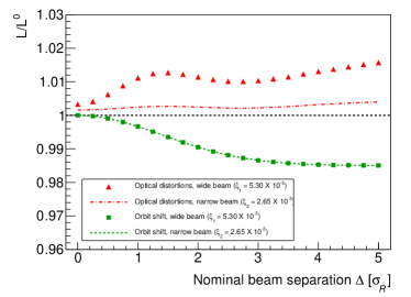
Figure 36: Single-beam contributions to the beam-separation dependence, during a horizontal  scan simulated using B*B, of the luminosity-bias factor associated with the optical distortions ($[\mathcal{L}/\mathcal{L}^{0}]_{\mathrm{Opt}}$, red curve and triangles), and of that induced by the beam-beam orbit shift ($[\mathcal{L}/\mathcal{L}^{0}]_{\mathrm{Orb}}$, green curve and squares). The unperturbed beams are assumed to be round and perfectly Gaussian. Their bunch populations are assumed equal ($n_{1}=n_{2}=0.78\times 10^{11}$ p/bunch), and their transverse beam sizes differ by a factor of $\sqrt{2}$ ($\sigma_{1}=99.6\,\mu$m, $\sigma_{2}=70.5\,\mu$m). The wide-beam contributions are shown by the filled markers, the narrow-beam contributions by the dashed curves. The beams collide only at the IP where the scan is taking place. The horizontal axis is the nominal beam separation in units of the effective transverse beam size $\sigma_{R}=\Sigma_{R}/\sqrt{2}$.

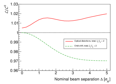
Figure 37: Beam-separation dependence, during a horizontal  scan simulated using B*B, of the luminosity-bias factor associated with the optical distortions ($[\mathcal{L}/\mathcal{L}^{0}]_{\mathrm{Opt}}$, red solid curve), and of that induced by the beam-beam orbit shift ($[\mathcal{L}/\mathcal{L}^{0}]_{\mathrm{Orb}}$, green dot-dashed curve), in the presence of a beam-size asymmetry corresponding to $\xi_{1}/\xi_{2}=2$. The single-beam parameters are listed in the caption of Fig. 36. The beams collide only at the IP where the scan is taking place. The horizontal axis is the nominal beam separation in units of the effective transverse beam size $\sigma_{R}=\Sigma_{R}/\sqrt{2}$.

To quantify the impact of a transverse beam-size asymmetry on beam-beam corrections to calibrations, the simulation protocol detailed above was repeated for several configurations in which the bunch populations were symmetric ($n_{1}=n_{2}=n$), the beam-size ratio $\sigma_{2}/\sigma_{1}$ was varied from 1.0 down to 0.65, and the convolved beam size was kept constant at $\Sigma_{R}=122\,\mu$m. Two values of the common bunch population were considered ($n=0.78\times 10^{11}$ and $n=1.21\times 10^{11}$ p/bunch), near the lower end, and beyond the upper end, of the bunch-intensity range used during scans; these translate into round-beam equivalent beam-beam parameter values of, respectively $\xi_{R}=3.53\times 10^{-3}$ and $5.50\times 10^{-3}$. The visible cross-section bias $\,\sigma_{\mathrm{vis}}/\,\sigma^{0}_{\mathrm{vis}}-1$ corresponding to each of these configurations, and computed from luminosity-bias curves such as those displayed in Fig. 37, is presented in Figs. 38 and 39.

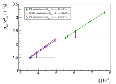
Figure 38: Dependence on the effective beam-beam parameter $\bar{\xi}$ of the visible cross-section bias $\,\sigma_{\mathrm{vis}}/\,\sigma^{0}_{\mathrm{vis}}-1$ associated with optical distortions, as predicted by B*B (diamonds) or COMBI (triangles) simulations, for low-intensity (open blue and red markers, bottom left) and high-intensity (filled green markers, top right) colliding-bunch configurations that cover a wide range of beam-size asymmetries at constant $\Sigma_{R}$ (see text). The beams collide at the scanning IP only. The $\,\sigma_{\mathrm{vis}}$ bias in the fully symmetric configuration ($\sigma_{1}=\sigma_{2}$) corresponds to the lowest value of $\bar{\xi}$ in each group, and is indicated by a horizontal black line. The curves are second-order polynomial fits to the points, and are intended to guide the eye. The arrows indicate the impact on the absolute luminosity scale of a 20% beam-size imbalance ($\sigma_{2}/\sigma_{1}=0.8$).

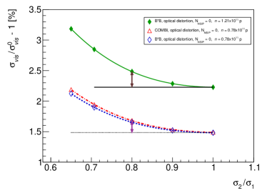
Figure 39: Dependence on the transverse beam-size ratio $\sigma_{2}/\sigma_{1}$ of the visible cross-section bias $\,\sigma_{\mathrm{vis}}/\,\sigma^{0}_{\mathrm{vis}}-1$ associated with optical distortions, as predicted by B*B (diamonds) or COMBI (triangles) simulations, for low-intensity (red and blue bottom curves) and high-intensity (green top curve) colliding-bunch configurations that cover a wide range of beam-size asymmetries at constant $\Sigma_{R}$ (see text). The beams collide at the scanning IP only. The $\,\sigma_{\mathrm{vis}}$ bias in the fully symmetric configuration ($\sigma_{1}=\sigma_{2}$) is indicated by a horizontal black line in each group. The curves are third-order polynomial fits to the points, and are intended to guide the eye. The arrows indicate the impact on the absolute luminosity scale of a 20% beam-size imbalance ($\sigma_{2}/\sigma_{1}=0.8$).

As the beam-size ratio deviates more and more from unity, $\bar{\xi}$ grows (see Eq. (45)), and so does the $\,\sigma_{\mathrm{vis}}$ bias. Its dependence on $\bar{\xi}$ is almost linear (Fig. 38), with only a small quadratic component. The scaling law, however, is approximate only, as evidenced by the slight relative misalignment of the B*B curves at the interface between the two groups ($\xi_{R}\sim 5.2$). The dependence on the beam-size ratio (Fig. 39) is well modeled by a third-order polynomial of $\sigma_{2}/\sigma_{1}$, the coefficients of which depend on the $n\,\beta^{*}$ product. A systematic difference between COMBI ands B*B becomes apparent at large asymmetry, suggesting that coherent oscillations may start to play a role in that regime. Quantitatively however, this discrepancy is small enough in the asymmetry range of interest at LHC (at most 0.01% on $\,\sigma_{\mathrm{vis}}$ for $\sigma_{2}/\sigma_{1}>0.9$, i.e. for an emittance imbalance of 20%) that it can be absorbed in a systematic uncertainty.

The impact of the beam-size asymmetry on the absolute luminosity scale, i.e. the difference in the $\,\sigma_{\mathrm{vis}}$ bias between a given asymmetric configuration (in this example $\sigma_{2}/\sigma_{1}=0.8$) and the fully symmetric case ($\sigma_{1}=\sigma_{2}$), is indicated by the arrows. The same results are presented in Fig. 40 (top three curves), on an expanded scale and after subtracting the $\,\sigma_{\mathrm{vis}}$ bias corresponding to the symmetric configuration.

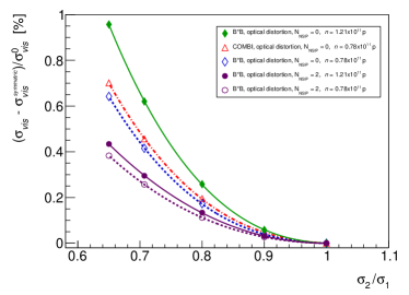
Figure 40: Impact of the beam-size asymmetry on the visible cross-section bias $\,\sigma_{\mathrm{vis}}/\,\sigma^{0}_{\mathrm{vis}}-1$ associated with optical distortions, as simulated using either B*B (diamonds and circles) or COMBI (triangles). Shown is the change is $\,\sigma_{\mathrm{vis}}$ bias between an asymmetric beam-beam configuration characterized by a given setting of $\sigma_{2}/\sigma_{1}<1$, and the corresponding symmetric configuration ($\sigma_{2}=\sigma_{1}$). The top three curves (green diamonds, red triangles and blue diamonds) correspond to the data displayed in Fig. 39, when the beams collide at the scanning IP only. The bottom two curves (circles) show the same results when the beams also collide head-on at two non-scanning IPs. The open (filled) symbols correspond to the low- (high-) intensity bunches (see text). The curves are third-order polynomial fits to the points, and are intended to guide the eye.

The results displayed in Figs. 36–39 assume that the beams collide at the scanning IP only. Additional collisions at other IPs lower the unperturbed tunes (Sec. 4.6.2): as a result, the impact of the beam–beam-induced optical distortion is significantly reduced (Fig. 12), and so is the impact of the transverse beam-size asymmetry. This is illustrated by the two bottom curves in Fig. 40, for the case of bunches colliding at two non-scanning IPs ($N_{\mathrm{NSIP}}=2$), that was modeled using B*B to simulate single-IP collisions but with the unperturbed tunes shifted as prescribed by Eq. (41). At the largest asymmetry considered ($\sigma_{2}/\sigma_{1}=0.65$), the sensitivity of the $\,\sigma_{\mathrm{vis}}$ bias to the beam-size asymmetry drops by more than a factor of two. In addition, the bunch-current dependence of this bias, manifested by the difference between the filled and the open circles, is several times smaller for the $N_{\mathrm{NSIP}}=2$ case. This occurs because the shift $\Delta\text{Q}_{\mathrm{mIP}}$ in unperturbed tunes is proportional to both $\xi$ and $N_{\mathrm{NSIP}}$: when both are large enough, this tune shift more than compensates the increase in optical distortion at the scanning IP associated with the increased beam-beam parameter experienced by the weaker of the two beams.

During Run-2 $pp$ scans at $\sqrt{s}=13$  TeV, the bunch population $n_{p}$ rarely exceeded $10^{11}$ (Table 1), and the typical beam-size asymmetry $\sigma_{2}/\sigma_{1}$ hovered around 0.94, as extracted from one of the non-factorization analyses outlined in Sec. 4.3.1. In practice therefore, for these sessions the impact of beam-beam asymmetries on beam-beam corrections to scans does not exceed 0.02% (Fig. 40); such a small number can be safely accounted for as a systematic uncertainty in the absolute luminosity scale.

5 Systematic uncertainties

Beam-beam (b-b)	$\xi_{\mathrm{s}im}$	Uncertainty-determination	$\,\sigma_{\mathrm{vis}}$ uncertainty [%]			Comments	See
uncertainty	$[10^{-3}]$	procedure	for $N_{\mathrm{NSIP}}$ =				Sec.
source			0	1	2
Absolute $\xi$ scale:	5.60	Vary $\,\beta^{*}$ by $\pm 10\%$ in the simulation	0.06	0.10	0.13	$\,\beta^{*}$ uncertainty assumed	4.2.1
$\,\beta^{*}$ uncertainty		or parameterization (Sec. 4.2.3),	(total for both beams			uncorrelated between beams,	+
at the scanning IP		for each beam and in each plane	and both planes)			correlated between planes	5.1.1
Nominal	5.60	Vary $\text{q}_{x}$, $\text{q}_{y}$ by $\pm 0.002$	0.26	0.23	0.20	Tune uncertainty assumed	4.2.2
collision tunes		in the simulation or parameterization,	(total for both beams			correlated between beams	+
		for each beam	and both planes)			and between planes	5.1.2
Non-Gaussian	5.60	B*B (or COMBI) simulations	0.13	0.22	0.30	Simulated for $N_{\mathrm{NSIP}}=0$,	4.3
transverse-density						extrapolated to $N_{\mathrm{NSIP}}\geq 1$	+
distributions						using Eq. (41)	5.2.1
Beam ellipticity	5.60	B*B (or COMBI) simulations.	$0.03$			Simulated for	4.4
at the scanning IP		Uncertainty scaled linearly				$\xi_{R}\leq 4.2\times 10^{-3}$,	+
		from $\xi_{R}$ to $\xi_{\mathrm{s}im}$				$0.7<\Sigma_{y}/\Sigma_{x}<1.4$	5.2.2
Non-zero	$\leq 5.60$	COMBI simulations	$<0.01^{*}$			for $\theta_{c}\leq 10\,\mu$rad∗	4.5 +
crossing angle			$<0.02~{}$			for $\theta_{c}\leq 150\,\mu$rad	5.2.3
Beam-beam	5.60	B*B and COMBI simulations	0.016∗	0.012∗	0.008∗	for $\sigma_{2}/\sigma_{1}>0.95^{*}$	4.7
imbalance			0.059	0.045	0.032	for $\sigma_{2}/\sigma_{1}>0.90~{}$	+
			0.136	0.104	0.072	for $\sigma_{2}/\sigma_{1}>0.85~{}$	5.2.4
Multiple IPs:
phase advance	5.60	COMBI (or B*B) simulations	0	$<0.20$		Worst case: arbitrary	4.6.4
						phase advances between IPs	+
multi-IP tune shift	5.60	Vary $p_{1}$ in Eq.(41) by $\pm 15\%$	0	0.05	0.09		4.6.5
		in single-IP simulations.					+
		Ignore if using multi-IP simulation					5.3
Long-range	-	None at the scanning IP	-				5.4.1
encounters		during $pp$ scans at the LHC
Lattice	-	COMBI simulations, with	0.01∗			for $E_{B}\geq 6.5$ TeV∗	5.4.2
non-linearities		sextupoles and octupoles included	0.03			at lower beam energies
Numerical accuracy	-		$<0.10$			Ignore if using simulation	5.4.3
of parameterization						rather than parameterization
Total uncertainty	5.60	Uncertainties summed in quadrature	$\pm 0.32$	$\pm 0.41$	$\pm 0.46$	% of $\,\sigma_{\mathrm{vis}}$	5.5
Total b-b correction	5.60	Parameterization (Secs. 4.2.3 & 4.6.5)	+0.52	+0.86	+1.17	% of $\,\sigma_{\mathrm{vis}}$	5.5

Table 8: Typical systematic uncertainties affecting beam-beam corrections to a hypothetical $pp$ calibration in a fully symmetric Gaussian-beam configuration, with the round–beam-equivalent beam-beam parameter set equal to $\xi_{\mathrm{s}im}$, for three values of $N_{\mathrm{NSIP}}$. For each source, the uncertainty is either evaluated at, or scaled linearly to, the value of $\xi_{\mathrm{s}im}$ indicated in the second column; if no value of $\xi_{\mathrm{s}im}$ is specified, the uncertainty listed covers the full range of $\xi$ values encountered during $pp$ scans at the LHC. When an uncertainty is assumption-dependent, the value flagged by an asterisk is that used in computing the total uncertainty; the latter is compared to the overall beam-beam correction itself in the bottom two rows of the Table. The rightmost column indicates the chapter(s) where the corresponding issues are discussed in detail.

The sources of systematic uncertainty that may affect the absolute magnitude of beam-beam corrections during scans, and that are detailed in Sec. 4, can be regrouped in three categories: optical configuration of the LHC rings, deviations from the fully symmetric Gaussian-beam configuration, and collisions at multiple IPs. The associated uncertainties are briefly elaborated upon in Secs. 5.1, 5.2 and 5.3 below; additional sources of potential bias are addressed in Sec. 5.4. All the uncertainties are then added in quadrature, and their combined magnitude compared in Sec. 5.5 to that of the overall beam-beam correction itself.

The quantitative impact of each uncertainty on the $\,\sigma_{\mathrm{vis}}$ bias, or equivalently on the magnitude of the beam-beam correction, is summarized in Table 8 for scans simulated using three different collision patterns ($N_{\mathrm{NSIP}}=0,1,2$). For each uncertainty source, the beam conditions input to the simulation are detailed in the chapters listed in the last column of the table. Not all simulations, however, use exactly the same beam conditions. In order to provide a self-consistent picture of the relative magnitude of the various uncertainties, and since the magnitude of the beam-beam bias, as well as most of the uncertainties, scale with $\xi$, the uncertainties listed in in Table 8 are all expressed at a common value $\xi_{\mathrm{s}im}$ of the beam-beam parameter; the details of this procedure can be found either in the table itself, or in Secs. 5.1 to 5.3. Because the chosen value of $\xi_{\mathrm{s}im}$ lies at the upper end of the range covered during Run-2 vdM scans, Table 8 illustrates something of a “worst-case” scenario with respect to the magnitude of the beam-beam correction and of the associated systematic uncertainty. The nmerical results listed in that table should therefore not be applied blindly to estimating actual -calibration uncertainties, but rather used as guidance for a case-by-case and bunch-by-bunch error analysis of actual -calibration data.

5.1 Optical configuration

5.1.1 $\,\beta^{*}$ uncertainty at the scanning IP

Since the $\,\sigma_{\mathrm{vis}}$ bias scales with the beam-beam parameter (Sec. 4.2), any measurement error on $\xi$ directly translates into an error of similar relative magnitude on beam-beam corrections to the luminosity scale. Existing accelerator instrumentation unfortunately does not allow accurate enough a determination of the transverse single-beam sizes that enter the definition of $\xi$ (Eq. (12)). The horizontal and vertical beam-beam parameters must therefore be redefined in terms of two-beam observables that can be reliably measured:

$$\xi_{xAv} = \frac{n\,r_{0}\,\beta^{*}_{xAv}}{\pi\,\gamma\,\Sigma_{x}(\Sigma_{x}+\Sigma_{y})}$$ (46)

$$\xi_{yAv} = \frac{n\,r_{0}\,\beta^{*}_{yAv}}{\pi\,\gamma\,\Sigma_{y}(\Sigma_{x}+\Sigma_{y})}\,.$$ (47)

Here, $\beta^{*}_{xAv}=(\beta^{*}_{x1}+\beta^{*}_{x2})/2$ is the beam-averaged horizontal $\beta$-function at the scanning IP, and similarly for $\beta^{*}_{yAv}$. The quantity $n=(n_{1}+n_{2})/2$ refers to the beam-averaged bunch population associated with the colliding-bunch pair under study, $\gamma=\gamma_{1}=\gamma_{2}$ is the common relativistic factor (assumed here to be the same for B1 and B2), and $\Sigma_{x}$ and $\Sigma_{y}$ are the convolved transverse bunch sizes. During scans, the observables $n$, $\Sigma_{x}$ and $\Sigma_{y}$ are measured on a bunch-by-bunch basis to sub-percent accuracy [38, 39, 40, 41], and the uncertainty on the absolute beam energy is totally negligible for the purposes of this paper. The main uncertainty affecting the absolute scale of the beam-beam parameter, therefore, is that associated with potential deviations of $\,\beta^{*}$ from its nominal or assumed value.

The facts that the $\xi$ dependence of the $\,\sigma_{\mathrm{vis}}$ bias is roughly linear (Fig. 16), and that the measured value of $\xi_{xj}$ (Eq. (12)) depends linearly on $n_{k}$ and $\beta^{*}_{xj}$ ($j,k=1,2;j\neq k$), justify the use of the beam-averaged variables defined in Eqs. (46)-(47) above. Furthermore, the very weak dependence of the $\,\sigma_{\mathrm{vis}}$ bias on the $\Sigma^{0}_{y}/\Sigma^{0}_{x}$ aspect ratio (Fig. 22) indicates that “averaging” over $x$ and $y$, in the sense of substituting the round-beam equivalent parameter $\xi_{R}$ (Eq. (28)) for the pair of horizontal and vertical beam-beam parameters ($\xi_{xAv},\xi_{yAv}$), results in an acceptably small bias. What finally matters, therefore, is the uncertainty on the beam- and plane-averaged value of $\,\beta^{*}$ at the scanning IP.

The $\,\beta^{*}$ values at the LHC IPs are extracted from optical-function measurements that are carried out for every colliding-beam configuration as part of routine accelerator commissioning. During the first few years of LHC operation, these values were typically obtained using the phase-advance method; k-modulation is now considered a more promising approach [47]. It targets an absolute accuracy of a few percent on $\beta^{*}_{iB}$ ($i=x,y$; $B=1,2$), provided sufficient beam time can be dedicated to the measurement.

The absolute $\,\beta^{*}$-accuracy requirements associated with beam–beam-correction uncertainties are rather modest. When beams collide at the scanning IP only, and for $\xi=5.6\cdot 10^{-3}$, a $\pm 10\%$ uncertainty in $\,\beta^{*}$ at the scanning IP, uncorrelated between beams (because the optics of the two rings are almost completely independent) but correlated between planes (because a focusing error presumably affects both the horizontal and the vertical $\beta$-function) results in $\pm 0.06\%$ uncertainty in $\,\sigma_{\mathrm{vis}}$ (Table 8). Treating this uncertainty as fully uncorrelated (correlated) between beams and between planes would decrease (increase) the corresponding $\,\sigma_{\mathrm{vis}}$ uncertainty by a factor of $\sqrt{2}$. The absolute uncertainty increases to 0.10% (0.13%) for $N_{\mathrm{NSIP}}=1(2)$, but its magnitude relative to the overall beam-beam correction remains about the same.

The $\pm 10\%$ $\,\beta^{*}$-uncertainty assumed in the example above is very conservative, and is representative of the typical difference between the nominal, i.e. the dialed-in, $\,\beta^{*}$ setting and the measured values. Smaller uncertainties can be achieved by calculating $\xi$ based on the measured $\,\beta^{*}$ values themselves, while accounting rigorously for the systematic $\,\beta^{*}$-measurement uncertainties and for their correlation between beams and between planes.

5.1.2 Nominal collision tunes

Figures 12 and 13 illustrate the sensitivity of the optical distortion and of the full beam-beam bias to the unperturbed fractional tunes. Any deviation of ($\text{q}_{x}$, $\text{q}_{y}$) from their nominal setting results in an inaccurate prediction of the $\,\sigma_{\mathrm{vis}}$ bias.

For the purposes of the present discussion, a conservative uncertainty of $\pm 0.002$ is assigned to each of $\text{q}_{x}$ and $\text{q}_{y}$, and is assumed to be correlated between beams (as could be caused by, for instance, instrumental effects) and between planes (because a focusing error presumably affects both the horizontal and the vertical betatron frequency). The magnitude of this uncertainty is based on LHC operational experience, and is meant to cover setting errors, as well as the stability of the unperturbed tunes, over the course of the -calibration fill(s). The corresponding uncertainty in $\,\sigma_{\mathrm{vis}}$ (Table 8) dominates the overall beam-beam uncertainty. It decreases slightly when the number of non-scanning IPs increases, because the additional collisions lower the unperturbed tunes, thereby reducing the sensitivity of the optical distortions to the exact values of the fractional tunes. The same effect is responsible for the $N_{\mathrm{NSIP}}$-dependent sensitivity of $\,\sigma_{\mathrm{vis}}$ to beam-beam asymmetries (Fig. 40).

5.2 Deviations from the fully symmetric Gaussian-beam configuration

Except where specifically stated otherwise, most of the results presented in this paper, and in particular the parameterizations detailed in Secs. 4.2.3 and 4.6.5, are based on the assumptions listed in Sec. 4.1. Each of these will be lifted, one at a time, in the following Sections, and their individual impact on beam–beam-correction uncertainties estimated using the studies detailed in Secs. 4.3 to 4.7.

5.2.1 Non-Gaussian unperturbed transverse-density profiles

Of the three single-bunch models described in Table 2, the 2012 parameter set represents an extreme case, both because this is the session that revealed the largest non-factorization biases at LHC ever [13, 40], and because the parameters in that Table are deliberately chosen to represent the worst case among all scans and all bunches in a given session. The 2018 model emerges as the most appropriate to estimate the uncertainty associated with non-Gaussian tails in the unperturbed density distributions: not only is the kurtosis intermediate between that of the other two parameter sets, but it also reflects the performance of the injector chain in the fourth year of LHC Run 2, by which time procedures had long stabilized and beam conditions could be considered reasonably reproducible.

Since the factorizable double-Gaussian configuration systematically yields a larger deviation from the corresponding single-Gaussian model than its non-factorizable counterpart (Table 4), it is favored for the purpose of estimating systematic errors. The uncertainty listed in Table 8 for $N_{\mathrm{NSIP}}=0$ is therefore taken from the top half of Table 4. It is extrapolated to the cases of one and two non-scanning IPs by assuming that the fractional impact of additional collisions on the $\,\sigma_{\mathrm{vis}}$ bias is dominated by the multi-IP tune shift (Sec. 4.6.2), and thus insensitive to the shape of the unperturbed transverse-density distributions.

The choice of the 2018 factorizable model to estimate the impact of non-Gaussian tails is not devoid of some arbitrariness. The uncertainties listed in Table 8, therefore, should be considered as a first indication, albeit a prudent one. A refined evaluation would require a more extensive characterization of the transverse-density distributions extracted from non-factorization analyses, that could then be used to produce a wider palette of more realistic single-bunch models for input to B*B or COMBI. In order to explore potential correlations between systematic biases, one could in addition extend the existing studies to simulate bunches that are not purely Gaussian and that in addition collide at multiple interaction points.

5.2.2 Beam ellipticity at the scanning IP

The dependence of the optical-distortion bias on the $\Sigma_{y}/\Sigma_{x}$ aspect ratio is summarized by Fig. 22, and does not exceed $\pm 0.025\%$ for $\xi_{R}\leq 4.2\cdot 10^{-3}$. Scaling this linearly to the value of $\xi_{\mathrm{s}im}$ shown in Table 8 yields a beam–beam-correction uncertainty of 0.03%, under the condition that the orbit-shift correction take the actual ellipticity into account, i.e. that it be computed using the Bassetti-Erskine formalism [6] with, as input, the measured values of $\Sigma_{x}$ and $\Sigma_{y}$.

5.2.3 Non-zero crossing angle

The crossing-angle dependence of the beam-beam bias in the regime is summarized by Fig. 23. The associated systematic uncertainty is taken as the difference in $\,\sigma_{\mathrm{vis}}$ bias between $\theta_{c}=0$ and the actual crossing-angle value; it is listed in Table 8 for two values of the full crossing angle.

It should be emphasized that this small uncertainty is applicable only at moderate crossing angles ($\theta_{c}\leq 150\,\mu$rad), and only in the regime ($\xi\leq 0.006$, $\,\beta^{*}\geq 10$ m). For larger crossing angles in the regime, additional effects may come into play. This may also be the case for scans performed in the physics regime, even at moderate crossing angle, when the beam-beam parameter becomes large enough, and/or when $\,\beta^{*}$ becomes small enough ($\,\beta^{*}\leq 30$ cm) for the hourglass effect to no longer be negligible. Of particular concern are the so-called “emittance scans”, that are -like beam-separation scans that are used to monitor luminometer performance and transverse emittances during routine LHC operation [48]: the study of their sensitivity to beam-beam-induced biases remains mostly unexplored territory.

5.2.4 Beam-beam imbalance

Of the three beam–beam-asymmetry scenarios considered in Sec. 4.7, only the transverse-emittance imbalance (Sec. 4.7.3) requires special attention, since bunch-current and $\,\beta^{*}$-asymmetries are accounted for by the use of the beam-averaged beam-beam parameters defined in Eqs. (46)-(47). The emittance-asymmetry dependence of the $\,\sigma_{\mathrm{vis}}$ bias is controlled by the combination of $\xi_{R}$ and of the transverse beam-size ratio $\sigma_{2}/\sigma_{1}$ (Eq. (45)); it also is sensitive to the number of non-scanning IPs (Fig. 40).

The beam–beam-imbalance uncertainty is taken as the difference in $\,\sigma_{\mathrm{vis}}$ bias between an asymmetric beam-beam configuration characterized by a given value of $\sigma_{2}/\sigma_{1}<1$, and the corresponding symmetric configuration ($\sigma_{2}=\sigma_{1}$); it is listed in Table 8 for three values of the transverse beam-size ratio. The ratio closest to unity ($\sigma_{2}/\sigma_{1}>0.95$), that emerged as the most representative of typical beam conditions during the 2015-2018 $pp$ sessions [40], is the one used when computing the total beam-beam uncertainty (penultimate row of Table 8). The $N_{\mathrm{NSIP}}$ dependence is discussed in Sec. 4.7.3, and is closely related to the tune-dependence of the optical-distortion bias (Sec. 5.1.2).

5.3 Multiple interaction points

Two sources of uncertainty affect the beam-beam correction strategies in the presence of multi-IP collisions, that are detailed in Sec. 4.6.6: the phase advance between consecutive IPs (Sec. 4.6.4), and the parameterization of the multi-IP equivalent tune shift $\Delta\text{Q}_{\mathrm{mIP}}$ (Sec. 4.6.5). These uncertainties affect only those colliding-bunch pairs in which at least one of the two opposing bunches experiences collisions at one or more IPs other than the scanning IP ($N_{\mathrm{NSIP}}>0$).

The phase-advance uncertainty arises from the currently unresolved ambiguity in the choice of the reference “no beam-beam” configuration, or, in more technical terms, from the ambiguity between the $\mathcal{L}^{0}$ and the $\mathcal{L}^{u}$ normalizations (Sec. 4.6.3). In the absence of any phase-advance information, e.g. for a bunch pattern that mixes different collision configurations that are all treated on the same footing, a blanket systematic uncertainty of at most 0.2% appears adequate (Sec. 4.6.4). This uncertainty can, in some cases, be significantly lowered by simulating the actual collision pattern associated with each colliding-bunch pair, with as input the actual IP-to-IP phase advance per beam and per plane, and by then comparing the results between the two reference no-beam configurations. An illustration of the potential gain provided by such a refined analysis is offered by the results presented in Table 7 for the $N_{\mathrm{NSIP}}=1$ case, a configuration that applies to the 13 TeV $pp$ scans at IP1 and IP5 in 2015, 2016 and 2017 [40].

The uncertainty associated with the equivalent multi-IP tune shift $\Delta\text{Q}_{\mathrm{mIP}}$ needs to be considered only when invoking the parameterization of single-IP simulations proposed in Sec. 4.6.5 and encapsulated in Eq. (41), to compute beam-beam corrections in the presence of additional collisions. This parametrization, that is illustrated by the magenta curve in Fig. 34, is in good agreement with the simulation results when IP5 is the scanning IP. The discrepancies that are apparent for scans at some of the other IPs, reflect the variety of phase-advance patterns between the scanning IP and the other collision points. Varying the $p_{1}$ parameter in Eq. (41) by $\pm 15\%$ of its central value covers all the collision patterns shown in Fig. 34, thereby providing a measure of the uncertainty associated with this simplified procedure (Table 8). More precise results, and a smaller uncertainty, could again be obtained by simulating separately each of the collision patterns associated with the B1 and B2 bunch strings circulating in the LHC ring during the -calibration session under analysis.

5.4 Other potential sources of systematic uncertainty

5.4.1 Long-range encounters

During $pp$ scans at the LHC, the bunches are longitudinally isolated, in the sense that consecutive bunches are separated by more than 500 ns, rather than grouped in trains with only 25 ns spacing. In addition, the fill pattern is systematically optimized to avoid parasitic crossings, at least at the scanning IP. This strategy eliminates separation-dependent, long-range beam-beam kicks that might distort the luminosity-scan curves.

In contrast, during high-luminosity $pp$ physics running, consecutive bunches are typically separated longitudinally by only 25 ns, the emittance is smaller than during scans, and the bunch current significantly larger. As a result, and in spite of the non-zero crossing angle, long-range beam-beam effects are known to significantly impact emittance scans in several ways, most of which remain to be understood.

5.4.2 Lattice non-linearities

The strongest non-linearity is introduced by the beam-beam interaction itself. However, non-linear magnetic elements in the LHC rings also affect beam dynamics, potentially leading to additional distortions of the transverse particle-density distributions. Because the LHC relies on the combination of high chromaticity ($Q^{\prime}\approx 10-15$ units) and of high Landau-octupole currents to mitigate some strong impedance-driven instabilities, the next largest optical non-linearities at beam energies above 1 TeV are associated with the corresponding sextupoles and octupoles [49]. As demonstrated experimentally [50, 51, 52], machine imperfections contribute even less by comparison, and are therefore neglected in the present study.

In order to quantify the impact of these magnets on the $\,\sigma_{\mathrm{vis}}$ bias, both the chromaticity and the linear detuning with amplitude introduced by the Landau octupoles were added to the COMBI model. The chromaticity dependence of the beam-beam bias is presented in Fig. 41 for two different beam energies. As expected, the impact of the octupoles is more important in the 2011 case because of the lower beam energy: at zero chromaticity, powering the octupoles changes the beam-beam bias from $-0.155\%$ to $-0.130\%$, a reduction in relative magnitude of about one sixth. In contrast, in the 2018 configuration the effect of the octupoles is three times smaller, and almost negligible. As for the chromaticity, its impact is negligible in both configurations.

The very low sensitivity of beam-beam corrections to these non-linear elements can be understood as follows. Octupoles act more strongly on larger-amplitude particles. These barely contribute to the luminosity when the beams collide head-on; the fractional contribution of the tails to the overlap integral is highest at large beam separation, but there the luminosity is the lowest. This is why modifying the trajectory of the tail particles barely influences the separation-integrated FoMs, and therefore the $\,\sigma_{\mathrm{vis}}$ bias.

Similarly, high chromaticity potentially enhances synchro-betatron coupling; however since scans are carried out with relaxed $\,\beta^{*}$ settings and at zero crossing angle, this is of no concern.

Even though lattice non-linearities are almost negligible in vdM scans (Table 8), it remains important to check systematically the potential influence of the octupoles under operational scenarios where they are pushed to maximum power to ensure beam stability: their impact on beam-beam uncertainties may turn out to be no longer negligible, for instance during emittance scans.

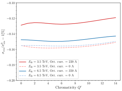
Figure 41: Chromaticity dependence of the $\,\sigma_{\mathrm{vis}}$ bias predicted by COMBI for $pp$ scans, with octupoles either under power (solid curves) or left at zero current (dashed curves). The red curves correspond to the 2011 configuration ($E_{B}=3.5$ TeV), the blue curves to that in 2018 ($E_{B}=6.5$ TeV); the corresponding octupole currents are indicated in the legend. The momentum spread and the synchrotron tune are set to, respectively, $1.12\text{\times}{10}^{-4}$ and $2\text{\times}{10}^{-3}$. The beam-beam parameter is set to $\xi=$2.6\text{\times}{10}^{-3}$$, and the beams collide at the scanning IP only.

5.4.3 Numerical accuracy of polynomial parameterization

Propagating to the $\,\sigma_{\mathrm{vis}}$ bias the parameterization uncertainties that affect the separation-dependent luminosity-bias factors (Eq. (27)) and that are discussed in Sec. 4.2.3, results in an upper limit of 0.1% on the associated beam-beam uncertainty. This contribution should be ignored when resorting to a full B*B or COMBI simulation at each scan point, rather than to the parameterization.

5.5 Summary of systematic uncertainties

Adding in quadrature all the above uncertainties yields, for the example examined here ($\xi_{\mathrm{s}im}=5.6\cdot 10^{-3}$), a total beam-beam uncertainty of 0.32 to 0.46%, depending on the number of non-scanning IPs (Table 8). The corresponding value of the beam-beam correction varies from 0.52 to 1.17%. The absolute magnitude of the total uncertainty grows when $N_{\mathrm{NSIP}}$ increases from 0 to 2, but its magnitude relative to the correction itself decreases from about 60% to roughly 40% through the mechanism dicussed in Secs. 5.1.2 and 5.2.4.

Under operating conditions typical of actual -calibration sessions, the number of non-scanning IPs is at least one. For $N_{\mathrm{NSIP}}=1$, the four dominant uncertainty contributions, in order of decreasing importance, are associated with the nominal tunes, non-Gaussian tails, multi-IP effects (in the absence of collision–pattern-specific studies), and the $\,\beta^{*}$ uncertainty. Estimating the uncertainty associated with non-Gaussian tails, and verifying whether beam-size asymmetries might contribute at a significant level, imperatively requires input from the non-factorization analysis of luminous-region data.

It is worth noting that the larger $N_{\mathrm{NSIP}}$, the larger the contribution of the orbit-shift correction relative to that of the optical distortion. Qualitatively therefore, estimating precisely the effects that contribute only to the optical-distortion uncertainty, viz. the beam ellipticity and the beam-size asymmetry, becomes less critical as the number of non-scanning IPs increases. In contrast, the $\,\beta^{*}$ and tune uncertainties affect the magnitude of both the orbit shift and the optical distortion, in a fully correlated manner.

The uncertainties detailed in Table 8 have been deliberately estimated in a conservative fashion, and for the largest value of the beam-beam parameter encountered during Run-2 scans in $pp$ collisions at $\sqrt{s}=13$ TeV. Most uncertainties scale with $\xi$, either linearly or with a slightly positive quadratic component. For the purposes of a rough estimate, therefore, they can be safely extrapolated linearly to smaller $\xi$ values, that are more representative of typical conditions. A more precise determination of these uncertainties requires a case-by-case analysis, possibly augmented by some of the additional simulation studies suggested in some of the preceding sections in this chapter.

6 Summary and outlook

Under conditions typical of luminosity-calibration scans in $pp$ collisions at the LHC, beam–beam-induced orbit shifts and optical distortions, if left uncorrected, bias the absolute luminosity scale by an amount comparable to, or larger than, the total luminosity-uncertainty budget. The magnitude of the correction, which ranges from approximately 0.2% to 1.2%, mainly depends on the beam-beam parameter $\xi$ and on the number of non-scanning IPs.

The contributions to the associated systematic uncertainty are listed in Table 8 and elaborated upon in Sec. 5.5. The total uncertainty amounts to roughly half of the correction itself, and is dominated by tune-related effects, either directly (accuracy and reproducibility of nominal-tune settings) or indirectly (beam-beam tune shift at non-scanning IPs, phase advance between consecutive IPs). The next most important source of uncertainty is the potential deviation of the unperturbed transverse bunch-density distributions from a perfectly Gaussian shape. Simulating the impact of non-Gaussian tails cannot be based on luminosity data alone: it requires, as input, single-bunch parameters that can only be extracted from the measured beam-separation dependence, during the scan, not only of the luminosity but also of the position, shape and orientation of the luminous region. These single-bunch parameters are also crucial to quantify transverse beam-size differences between the two beams, which, if large enough, may become a significant source of uncertainty.

The scope of the present paper is limited to beam-separation scans in the regime ($\xi\leq 6\cdot 10^{-3}$), under beam conditions that deviate only moderately from round, initially Gaussian bunches of equal brightness that collide with a zero or small nominal crossing angle. In the course of investigating the impact of actual departures from that idealized limit, several areas of further study have been identified, most notably:

• improved single-bunch models of non-Gaussian tails (Sec. 4.3), both factorizable and non-factorizable, that are more sophisticated than the simple double-Gaussian functions considered in Eqs. (36) and (37);

• the interplay between non-factorization, non-Gaussian tails, and beam-beam corrections, and in particular the application of beam-beam corrections to two-dimensional grid scans;

• the ambiguity affecting the choice of the reference “no beam-beam” configuration, i.e. the phase-dependence of the difference between the $\mathcal{L}^{0}$ and the $\mathcal{L}^{u}$ normalizations (Sec. 4.6);

• the characterization of optical distortions at large nominal crossing angle (Sec. 4.5) in the regime;

• the potential interplay between the impact of non-Gaussian beams (Sec. 4.3), beam ellipticity (Sec. 4.4), crossing angle (Sec. 4.5), and multi-IP effects (Sec. 4.6), that have so far been treated as fully uncorrelated;

• the extension of the $\xi$-scaling laws (Sec. 4.2) to the physics regime ($\xi\leq 10^{-2}$), with emittance scans as the primary use case;

• the combined impact, during emittance scans at low $\,\beta^{*}$ in the physics regime, of higher-beam-beam parameter values and of the hourglass effect on the crossing-angle dependence of beam-beam biases;

• the impact of parasitic crossings on the absolute accuracy of emittance scans during routine physics running;

• the impact of lattice non-linearities on the absolute accuracy of emittance scans during routine physics running.

7 Acknowledgments

We thank our colleagues in the LHC Luminosity Monitoring and Calibration Working Group (LLCMWG), and in particular V. Balagura, X. Buffat, R. Hawkings, W. Herr and J. Wenninger, for many fruitful discussions and for valuable comments on part or all of the manuscript. We are also indebted to V. Balagura for teaching us how to run his B*B package, as well as for implementing additional functionalities needed by the studies reported above. Some of the authors have received support from either the Swiss Accelerator Research and Technology Institute (CHART), the U.S. Department of Energy (DOE Contract No. DE-AC02-76SF00515), or the Hungarian National Research, Development and Innovation Office (NKFIH Contract Nos. 124845 and 143460).

Appendix A Impact of non-Gaussian distortions of the source field

Because B*B is fundamentally a weak-strong model, beam–beam-induced shape-distortions of the witness bunch, i.e. of the multiparticle distribution, influence neither the shape of the source bunch nor the spatial dependence of the electromagnetic field it generates. The latter is computed once and for all at initialization time, and remains static both turn-by-turn and as a function of beam separation.

COMBI, in contrast, is based on a strong-strong model: both bunches are represented by macroparticles; both play, with respect to their partner, the dual roles of source and witness bunch; and the electromagnetic fields they generate are updated on a turn-by-turn basis, and therefore also at each scan step. In order to estimate the impact of separation-dependent, non-Gaussian field distortions caused by the mutual interaction of the opposing bunches, the $\,\sigma_{\mathrm{vis}}$ bias (Eq. (34)) has been computed using COMBI in two different modes:

• for each witness bunch in turn, the field that its macropraticles are subjected to, is computed under the assumption that the transverse macroparticle distribution of the source bunch is a two-dimensional Gaussian, with the position of its centroid and its RMS widths computed on every turn from the actual spatial distribution of the “source” macropraticles. This procedure tracks the evolution of the relative position and of the width of the opposing multiparticle distributions, but the field calculation ignores potential deviations of the bunches from their initial, perfectly Gaussian shape. This is the mode in which all the COMBI results in this paper have been obtained.

• for each witness bunch, the field it is subjected to is computed by the HFMM method [34] from the actual charge distribution in the source bunch. In this mode, each macroparticle in the witness bunch is subjected to an electromagnetic field computed as the vector sum of the contributions of all the macroparticles in the source bunch. Since this computation must be repeated on every turn and for the opposing bunch, it is much more CPU-intensive than the Gaussian-field approximation above.

Figure 42 displays the beam–beam-parameter dependence of the $\,\sigma_{\mathrm{vis}}$ bias over a $\xi$ range that extends all the way up to $25\times 10^{-3}$, more than four times the highest $\xi$ value encountered in scans, and significantly higher than the largest per-IP beam-beam parameter that is sustained operationally in the actual LHC rings. The two calculations agree within 1% or better; for the $\xi$ range and the nominal tunes considered in Table 1, this translates into a $\,\sigma_{\mathrm{vis}}$ difference of less than 0.005%. Computing the electromagnetic field as that of an equivalent Gaussian, the parameters of which evolve turn by turn, therefore constitutes a fully justified approximation whose impact on beam-beam corrections can be safely neglected.

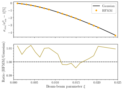
Figure 42: Top: $\xi$ dependence of the beam-beam induced $\sigma_{vis}$ bias, computed either in the Gaussian-kick approximation (solid black line), or with a self-consistent kick calculated using the HFMM field solver (filled orange circles). Bottom: $\xi$ dependence of the ratio between the $\,\sigma_{\mathrm{vis}}$-bias values computed by the two methods.

Appendix B Luminosity Integration in COMBI

In COMBI, the calculation of the luminosity, or more precisely of the overlap integral (Eq. (1)), is based on a complete description of the macroparticle distribution in the two colliding bunches: no assumption is made about the shape of the density distributions when evaluating this integral. The latter is calculated on a turn-by-turn basis, both at the scanning IP and at the non-scanning IP(s), if any. The positions of all the macroparticles are updated at each IP on every consecutive turn, and each step in a beam-separation scan is initialized and simulated separately.

The transverse distribution of the macroparticles, called $H^{B}_{x,y}$, is discretized, separately for the two beams $B$ ($B=1,2$), on a two-dimensional grid in the $x$-$y$ plane. The number of cells in each grid is given by $N_{\mathrm{cells}}=n\times m$, where $n$ and $m$ represent the number of bins in the $x$ and $y$ directions respectively. The grid boundaries are located at a distance $k_{i}\times\sigma^{0}_{i}$ ($i=x,y$) from the center of the grid, where $\sigma^{0}_{i}$ is the initial, unperturbed nominal transverse beam size inferred from the input emittance and $\,\beta^{*}$ values in the $i$ plane; the scale factor $k_{i}$ is typically set to 12 in both the positive and the negative direction along the $x$ and $y$ axes. The cell area is thus given by

$$\Delta S=\Delta x\times\Delta y=2k_{x}\sigma^{0}_{x}/n\times 2k_{y}\sigma^{0}_{y}/m\,.$$

The separation between the two beams is taken into account when filling two-dimensional histograms of the macroparticle distributions.

With these definitions, the discretized macroparticle density distribution is given by

$$h_{x,y}^{B}=\frac{H^{B}_{x,y}}{N_{part}\,\Delta S}\,,$$

where $N_{part}$ is the total number of tracked macroparticles. The overlap density of the two bunches, i.e. the product $\hat{\rho}_{1}(x,y)\,\hat{\rho}_{2}(x,y)$ in Eq. (1), is therefore represented by:

$$\lambda_{x,y}=h^{1}_{x,y}h^{2}_{x,y}\,.$$

The bunch luminosity can be calculated from the overlap integral $I_{\mathrm{ovlp}}$ as:

$$\mathcal{L}_{\mathrm{b}}=f_{\mathrm{r}}\,n_{1}n_{2}\,I_{\mathrm{ovlp}},$$ (48)

where $n_{1}$ and $n_{2}$ are the bunch populations and $f_{\mathrm{r}}$ the revolution frequency. The overlap integral is estimated by the two-dimensional trapezoidal method:

$$I_{\mathrm{ovlp}} \simeq \frac{1}{4}\Delta x\Delta y\Biggl{(}\lambda_{0,0}+\lambda_{m,0}+\lambda_{0,n}+\lambda_{m,n}+$$

$$2\sum_{i=1}^{m-1}\lambda_{i,0}+2\sum_{i=1}^{m-1}\lambda_{i,n}+2\sum_{j=1}^{n-1}\lambda_{0,j}+$$

$$2\sum_{j=1}^{n-1}\lambda_{m,j}+4\sum_{j=1}^{n-1}\Biggl{(}\sum_{i=1}^{m-1}\lambda_{i,j}\Biggr{)}\Biggr{)}.$$

The instantaneous luminosity in Eq. (48) is calculated at each turn, and the result is averaged over the total number of selected turns. Typically a few hundred turns are necessary for the result to stabilize. The reliability of this method was confirmed by benchmarking it against analytical calculations, with the beam-beam effects turned off.

Figure 43 shows the evolution of the $\,\sigma_{\mathrm{vis}}$ bias as a function of the number of macroparticles used in the simulation. The result converges to within 0.01% of its asymptotic value for $5\times 10^{6}$ macroparticles. Most of the simulation results presented in this paper are based on $10\times 10^{6}$ macroparticles per bunch, implying that the results are numerically stable at the $0.001\%$ level.

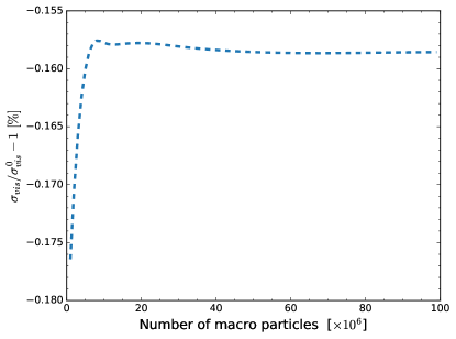
Figure 43: Visible cross-section bias as a function of the number of macroparticles used to model the transverse-density distributions.

The uncertainty associated with statistical fluctuations in the discretization of the transverse-density distributions was evaluated separately, and typically cancels out when computing luminosity ratios such as $[\mathcal{L}/\mathcal{L}^{0}]$. It becomes significant only at large beam separation, when the overlap integral is computed from a small number of macroparticles in the tails. At these scan points, however, the luminosity values are very small, and therefore have a negligible impact on the estimation of the beam-beam bias factors.

Appendix C Parameterization of optical-distortion corrections

Horizontal scans	Vertical scans
$0.002\leq\xi_{R}\leq 0.007$
$0.2975\leq\text{q}_{x}\leq 0.3100$	$\text{q}_{y}-0.0125\leq\text{q}_{x}\leq\text{q}_{y}-0.0075$
$\text{q}_{x}+0.0075\leq\text{q}_{y}\leq\text{q}_{x}+0.0125$	$0.3075\leq\text{q}_{y}\leq 0.3200$

Table 9: Parameter space used in the determination of the $[\mathcal{L}/\mathcal{L}^{0}]_{\mathrm{Opt}}$ polynomial coefficients.

The polynomial parameters $p_{0k},...,p_{9k}$ from which to calculate the optical-distortion luminosity-bias factor

$$[\mathcal{L}/\mathcal{L}^{0}]_{\mathrm{Opt}}(\xi_{R},\text{q}_{x},\text{q}_{y}|\Delta_{k})=p_{0k}+p_{1k}\,\xi_{R}$$

$$+p_{2k}\,\text{q}_{x}+p_{3k}\,\text{q}_{y}+p_{4k}\,\xi_{R}^{2}+p_{5k}\,\text{q}_{x}^{2}+p_{6k}\,\text{q}_{y}^{2}$$

$$+p_{7k}\xi_{R}\text{q}_{x}+p_{8k}\,\xi_{R}\,\text{q}_{y}+p_{9k}\,\text{q}_{x}\,\text{q}_{y}$$ (49)

defined in Eq. (27) of Sec. 4.2.3, have been tabulated, for normalized nominal-separation values covering the range $0<|\Delta_{k}/\sigma_{0}|<6$ in steps of 0.25. Here the index $k$ ($k=$ 1, 25) labels the nominal-separation bin $\Delta_{k}$ in the scanning plane considered. This parameterization is valid in the fully symmetric Gaussian-beam configuration with zero non-scanning IPs, over the three-dimensional space of fractional tunes ($\text{q}_{x}$, $\text{q}_{y}$) and round–beam-equivalent beam-beam parameter $(\xi_{R})$ values defined in Table 9. The values of $\,\beta^{*}$, $\gamma$, $\sigma_{0}$ and $n$ in Eq. (13) were chosen such that they correspond to typical settings for $pp$ -calibration sessions during Run 2 of the LHC.

The coefficients $p_{0k},...,p_{9k}$ are listed in Tables 10 and 11 for horizontal and vertical scans, respectively; they are also publicly accessible, in computer-readable form, in Ref. [37]. In the unabridged tables, i.e. for the studies reported in Secs. 4.2.3 and 4.2.4, all parameters were stored with a number of digits corresponding to the precision of the IEEE 754 double-precision floating-point data format. In the tables below, the coefficients are listed with enough precision to reproduce the values of $[\mathcal{L}/\mathcal{L}^{0}]_{\mathrm{Opt}}$ in the unabridged tables to at least five decimal digits. For verification purposes, $50\times 10^{3}$ points were randomly chosen across the $(\xi_{R},\text{q}_{x},\text{q}_{y})$ space defined in Table 9, and for each of these, 200 $\Delta$ values were randomly generated. The resulting $[\mathcal{L}/\mathcal{L}^{0}]_{\mathrm{Opt}}$ values, obtained using the unabrigded tables or the ones below, were then compared. The maximum differences found in $10\times 10^{6}$ evaluations were $5.4\times 10^{-6}$ and $9.5\times 10^{-6}$ for horizontal and vertical scans, respectively.

The procedure to correct an $x$-$y$ pair of experimentally measured -scan curves for beam–beam-induced optical distortions is detailed below. It is valid only for on-axis, one-dimensional scans with zero crossing angle; off-axis one-dimensional scans, as well as two-dimensional grid scans in the $(\delta_{x},\delta_{y})$ beam-separation plane, require dedicated simulations.

1. For a given colliding-bunch pair, calculate the values of $\sigma_{R}$ and $\xi_{R}$ from the measured bunch-current and uncorrected ($\Sigma_{x}$, $\Sigma_{y}$) values, following the prescriptions in Sec. 4.2.3;

2. for that same bunch pair, calculate the values of the effective fractional tunes ($\text{q}_{x}$, $\text{q}_{y}$), following the prescription in Sec. 4.6.5 with, as input, the nominal tune values ($\text{Q}_{x}$, $\text{Q}_{y}$), the appropriate number $N_{\mathrm{NSIP}}$ of non-scanning IPs, and the resulting multi-IP equivalent tune shift $\Delta\text{Q}_{\mathrm{mIP}}$;

3. for each scanning plane ($x$ and $y$) and each tabulated value of the nominal separation $\Delta_{k}$, calculate the corresponding value of $\{[\mathcal{L}/\mathcal{L}^{0}]_{\mathrm{Opt}}\}_{k}=[\mathcal{L}/\mathcal{L}^{0}]_{\mathrm{Opt}}(\xi_{R},\text{q}_{x},\text{q}_{y}|\Delta_{k})$ using Eq. (49), with the polynomial coefficients taken from the relevant row of Table 10 or 11, as appropriate;

4. use all pairs of numbers $(\Delta_{k},\{[\mathcal{L}/\mathcal{L}^{0}]_{\mathrm{Opt}}\}_{k})$ as input to a suitably chosen numerical-interpolation algorithm that can return the value of $[\mathcal{L}/\mathcal{L}^{0}]_{\mathrm{Opt}}(\Delta/\sigma_{R})$ for any nominal separation $\Delta$;

5. at each scan step, multiply the measured collision rate by $1/[\mathcal{L}/\mathcal{L}^{0}]_{\mathrm{Opt}}(\Delta/\sigma_{R})$, where $\Delta$ is the nominal separation for the scan step and in the scanning plane considered. This final step yields, for the bunch pair considered, the horizontal and vertical -scan curves corrected for optical distortions.

$\Delta_{k}[\sigma_{0}]$	$p_{0k}$	$p_{1k}$	$p_{2k}$	$p_{3k}$	$p_{4k}$	$p_{5k}$	$p_{6k}$	$p_{7k}$	$p_{8k}$	$p_{9k}$
0.00	1.00944	-9.9169	0.05163	-0.10946	-11.343	0.27849	0.51631	17.907	17.933	-0.70617
0.25	1.0965	-11.2335	-0.37109	-0.25749	-15.156	0.8075	0.59757	21.37	19.207	-0.38121
0.50	1.33057	-14.2614	-1.41804	-0.75044	-23.614	2.23701	1.09972	29.115	22.489	0.21938
0.75	1.6732	-18.353	-3.14234	-1.28652	-32.777	4.71339	1.58581	37.476	28.876	0.9846
1.00	2.09627	-23.4765	-4.63004	-2.55265	-38.221	3.68123	0.36501	50.199	34.146	7.71504
1.25	2.35234	-28.0037	-5.75125	-3.10402	-38.905	3.96085	-0.21768	57.845	41.93	10.74776
1.50	2.5998	-30.8986	-6.20145	-4.24446	-36.073	8.14783	4.83319	59.119	50.075	4.06889
1.75	2.71221	-32.1903	-5.80054	-5.33954	-33.326	6.80135	5.92624	54.751	58.075	5.3906
2.00	2.68384	-31.9924	-4.60368	-6.30519	-25.565	5.92361	8.49128	47.367	63.795	3.25386
2.25	2.72577	-30.6931	-4.15275	-7.00444	-15.931	4.41796	8.97022	42.853	63.188	4.6426
2.50	2.71357	-29.8333	-3.31831	-7.7255	-17.797	-0.48377	6.79757	35.712	67.066	11.47357
2.75	2.55328	-28.5073	-2.93845	-7.07616	-19.558	2.2039	8.83346	28.805	69.588	5.10042
3.00	2.63081	-28.984	-3.48143	-7.0339	-13.235	1.7513	7.59532	37.803	62.493	7.5962
3.25	2.51794	-29.2876	-3.37658	-6.41585	-9.579	2.73257	7.63313	38.021	63.687	5.42281
3.50	2.57552	-30.733	-3.87832	-6.30735	-5.79	3.30687	7.27443	49.126	58.156	5.87508
3.75	2.7132	-34.1604	-4.72201	-6.34866	0.329	4.88899	7.5148	62.801	56.443	5.47604
4.00	2.80473	-36.4992	-6.20828	-5.49987	-0.487	1.89557	1.09204	77.16	50.842	15.98952
4.25	2.84402	-40.437	-7.01717	-4.94963	5.671	5.45919	2.26449	89.531	51.974	11.6835
4.50	2.92941	-42.1662	-7.69945	-4.84568	7.414	12.10344	7.25898	100.023	47.916	1.02831
4.75	3.00531	-44.2824	-8.94959	-4.12019	4.043	8.3604	0.8071	119.399	36.595	12.11431
5.00	3.1174	-47.4622	-9.45872	-4.32462	10.289	7.49102	-0.57319	125.029	41.518	15.50293
5.25	3.08992	-48.0346	-9.55933	-4.06527	9.796	14.24273	5.29776	139.651	29.582	2.65662
5.50	3.22545	-51.1449	-10.7063	-3.79323	9.956	14.35667	3.04625	141.488	38.024	6.20924
5.75	3.25358	-51.7947	-11.62684	-3.08922	7.899	12.51096	-1.17893	151.272	30.874	12.68129
6.00	3.15344	-50.9016	-10.84895	-3.228	7.762	19.8657	7.03849	145.734	33.547	-3.89875

Table 10: Parameterization of the $[\mathcal{L}/\mathcal{L}^{0}]_{\mathrm{Opt}}$ luminosity-bias factor as a function of the normalized nominal separation, for horizontal scans. The functional form is defined in Eq. (49).

$\Delta_{k}[\sigma_{0}]$	$p_{0k}$	$p_{1k}$	$p_{2k}$	$p_{3k}$	$p_{4k}$	$p_{5k}$	$p_{6k}$	$p_{7k}$	$p_{8k}$	$p_{9k}$
0.00	1.00627	-9.8954	0.02224	-0.06076	-11.359	0.0568	0.18622	17.901	17.872	-0.18399
0.25	1.20592	-12.0782	-0.02827	-1.29247	-17.815	0.1942	2.21186	19.01	24.368	-0.28862
0.50	1.75762	-17.6722	-0.35287	-4.51951	-30.505	-0.9264	5.84403	22.471	40.37	2.91383
0.75	2.47795	-24.582	-0.92069	-8.60293	-41.735	1.3187	13.56868	20.768	65.956	0.45508
1.00	3.16343	-32.8235	-1.16788	-12.75235	-55.11	-0.3834	18.27023	29.422	85.709	4.49981
1.25	3.74028	-38.7998	-2.36278	-15.28112	-48.5	0.3875	21.25607	39.51	95.711	6.74987
1.50	3.96499	-42.0778	-3.06102	-16.01822	-37.845	-1.1981	19.73221	36.839	108.559	12.15308
1.75	3.69522	-40.042	-3.62485	-13.73364	-31.695	-1.4007	14.95999	39.742	98.388	14.38483
2.00	3.17695	-34.3599	-3.98479	-10.06481	-23.614	5.9537	15.52287	48.181	70.742	1.19056
2.25	2.54203	-27.8488	-4.42917	-5.57026	-15.667	5.2247	6.89102	46.516	50.153	4.09602
2.50	1.93646	-21.3641	-4.22219	-1.90718	-15.994	5.1956	1.34853	47.557	27.611	3.48476
2.75	1.64684	-18.4268	-4.50556	0.22396	-11.197	5.0949	-2.57366	49.259	16.174	4.5606
3.00	1.58403	-17.9608	-4.4421	0.56159	-7.635	6.066	-2.11206	48.03	16.126	2.48878
3.25	1.84422	-21.9484	-4.56541	-0.96411	-2.223	3.7746	-2.00762	49.005	28.617	7.28473
3.50	2.32149	-27.3088	-4.57251	-4.00249	1.528	4.2728	3.31839	48.531	47.316	6.31746
3.75	2.86007	-35.4916	-3.79586	-8.17387	13.02	7.1856	13.85154	44.04	78.901	-1.77626
4.00	3.52241	-43.4275	-3.74323	-12.44714	15.761	2.4115	16.29906	43.702	105.987	7.26694
4.25	4.18491	-52.8584	-3.75654	-16.63881	17.478	2.9322	23.4521	43.277	137.933	6.26266
4.50	4.82121	-61.3184	-4.12935	-20.31864	25.852	-1.7901	24.22835	37.512	171.614	16.6589
4.75	5.33928	-68.7429	-4.41872	-23.34458	24.7	3.8166	33.91458	37.937	196.185	6.67136
5.00	5.80246	-73.1287	-3.19177	-27.51882	20.495	18.7373	56.57897	38.918	210.435	-26.21613
5.25	6.44223	-79.2346	-5.10161	-29.74714	33.649	17.5226	56.18781	50.413	219.306	-17.92498
5.50	7.17335	-86.1747	-5.53665	-33.9533	35.037	6.9886	52.15683	35.086	257.011	3.99827
5.75	6.8188	-87.1346	-4.86936	-32.37045	28.729	-1.12	43.18943	42.423	253.701	17.49413
6.00	6.41896	-87.7396	-0.88027	-33.73032	32.935	1.0047	53.37414	28.725	269.298	0.87602

Table 11: Parameterization of the $[\mathcal{L}/\mathcal{L}^{0}]_{\mathrm{Opt}}$ luminosity-bias factor as a function of the normalized nominal separation, for vertical scans. The functional form is defined in Eq. (49).

References

- [1] P. Grafström and W. Kozanecki “Luminosity Determination at Proton Colliders” In Progr. Part. Nucl. Phys. 81, 2015, pp. 97–148 DOI: 10.1016/j.ppnp.2014.11.002
- [2] S. van der Meer “Calibration of the effective beam height in the ISR”
- [3] C. Rubbia “Measurement of the Luminosity of Collider with a (generalized) van der Meer Method”
- [4] W. Herr “Beam-beam effects and dynamic ”
- [5] ATLAS Collaboration “Improved luminosity determination in collisions at = 7 TeV using the ATLAS detector at the LHC” In Eur. Phys. J. C 73, 2013, pp. 2518 DOI: 10.1140/epjc/s10052-013-2518-3
- [6] M. Bassetti and G.. Erskine “Closed Expression for the Electrical Field of a Two-dimensional Gaussian Charge”
- [7] “MAD (Methodical Accelerator Design) home page” URL: https://madx.web.cern.ch/madx/
- [8] V. Balagura “van der Meer scan luminosity measurement and beam–beam correction” In Eur. Phys. J. C 81, 2021, pp. 26 DOI: 10.1140/epjc/s10052-021-08837-y
- [9] “COMBI (COherent Multibunch Beam-beam Interactions) home page” URL: https://twiki.cern.ch/twiki/bin/view/ABPComputing/COMBI
- [10] V. Balagura “Notes on van der Meer scan for absolute luminosity measurement” In Nucl. Instr. Meth. A 654, 2011, pp. 634–638 DOI: 10.1016/j.nima.2011.06.007
- [11] Y. Cai “Luminosity of Asymmetric e+e- Collider with Coupling Lattices” arXiv:hep-ph/0007052 [hep-ph]
- [12] K. M. Potter and J. C. Sens (editors) “Luminosity and Particle detection studies at the CERN Intersecting storage Rings” Internal Report CERN-NP-71-6 (1971)
- [13] ATLAS Collaboration “Luminosity determination in collisions at = 8 TeV using the ATLAS detector at the LHC” In Eur. Phys. J. C 76, 2016, pp. 653 DOI: 10.1140/epjc/s10052-016-4466-1
- [14] W. Herr and B. Muratori “Concept of luminosity” In CERN Accelerator School and DESY Zeuthen: Accelerator Physics, 2003, pp. 361–377
- [15] S. Peggs “Beam-beam collisions and crossing angles in RHIC” URL: http://www.osti.gov/servlets/purl/11446-VJM6RV/webviewable/
- [16] A. Chao, K.-H. Mess, M. Tigner and F. Zimmermann “Handbook of Accelerator Physics and Engineering” WORLD SCIENTIFIC, 2nd ed., 2013 DOI: 10.1142/8543
- [17] J. Wenninger “Operation and Configuration of the LHC in Run 2”
- [18] P. Bambade et al. “Observation of beam-beam deflections at the interaction point of the SLAC Linear Collider” In Phys. Rev. Lett. 62, 1989, pp. 2949–2952 DOI: 10.1103/PhysRevLett.62.2949
- [19] V. Ziemann “Beyond Bassetti and Erskine: Beam-beam deflections for non-Gaussian beams” In 7th Beam Dynamics Workshop, 1991, pp. 36–42
- [20] W. Kozanecki, T. Pieloni and J. Wenninger “Observation of Beam-beam Deflections with LHC Orbit Data”
- [21] S.-Y. Lee “Accelerator Physics” WORLD SCIENTIFIC, 4th ed., 2018 DOI: 10.1142/11111
- [22] W. Herr and T. Pieloni “Beam-Beam Effects” In Contribution to the CAS - CERN Accelerator School: Advanced Accelerator Physics Course, Trondheim, Norway, 18-29 Aug 2013
- [23] A.. Chao, P. Bambade and W.. Weng “Nonlinear beam-beam resonances” In Joint US / CERN School on Particle Accelerators: Topical Course on Nonlinear Dynamics, SLAC-PUB-3545 (1985)
- [24] A.. Chao “Beam-beam instability” In AIP Conf. Proc. 127, 1985, pp. 201–242
- [25] R. Tomás et al. “Beam-beam amplitude detuning with forced oscillations” In Phys. Rev. Accel. Beams 20, 2017, pp. 101002 DOI: 10.1103/PhysRevAccelBeams.20.101002
- [26] T. Pieloni “A study of beam-beam effects in hadron colliders with a large number of bunches”, 2008 DOI: 10.5075/epfl-thesis-4211
- [27] T. Pieloni and W. Herr “Models to study multibunch coupling through head-on and long-range beam-beam interactions”
- [28] T Pieloni and W Herr “Coherent Beam-Beam Modes in the CERN Large Hadron Collider (LHC) for Multiple Bunches, Different Collision Schemes and Machine Symmetries” DOI: 10.1109/PAC.2005.1591706
- [29] F. Jones, W. Herr and T. Pieloni “Parallel Beam-Beam Simulation Incorporating Multiple Bunches and Multiple Interaction Regions”
- [30] X. Buffat “Transverse beams stability studies at the Large Hadron Collider”, 2015 DOI: https://doi.org/10.5075/epfl-thesis-6321
- [31] “Open MPI home page” URL: https://www.open-mpi.org
- [32] K. Hirata “Who is afraid of a crossing angle?”
- [33] L. Barraud and X. Buffat “Mode coupling instability of colliding beams in the HL-LHC”
- [34] W. Herr, M.. Zorzano and F. Jones “Hybrid fast multipole method applied to beam-beam collisions in the strong-strong regime” In Phys. Rev. ST Accel. Beams 4 American Physical Society, 2001 DOI: 10.1103/PhysRevSTAB.4.054402
- [35] CMS Collaboration “CMS luminosity measurement for the 2018 data-taking period at ,TeV”
- [36] CMS Collaboration “CMS luminosity measurement using nucleus-nucleus collisions at in 2018”
- [37] A. Babaev et al. “Parameterization of beam–beam-induced optical distortions of van der Meer scans at the LHC” Zenodo, 2023 DOI: 10.5281/zenodo.8033453
- [38] LHCb collaboration “Precision luminosity measurements at LHCb” In Journal of Instrumentation 9.12, 2014, pp. P12005 DOI: 10.1088/1748-0221/9/12/P12005
- [39] CMS Collaboration “Precision luminosity measurement in proton–proton collisions at = 13 TeV in 2015 and 2016 in CMS” In Eur. Phys. J. C 81, 2021, pp. 800 DOI: 10.1140/epjc/s10052-021-09538-2
- [40] ATLAS Collaboration “Luminosity determination in collisions at TeV using the ATLAS detector at the LHC” DOI: 10.48550/ARXIV.2212.09379
- [41] ALICE Collaboration “ALICE 2016-2017-2018 luminosity determination for pp collisions at TeV”
- [42] H. Bartosik and G. Rumolo “Production of the single bunch for Van der Meer scans in the LHC injector chain”
- [43] R.. Workman “Review of Particle Physics” In PTEP 2022, 2022, pp. 083C01 DOI: 10.1093/ptep/ptac097
- [44] A. Babaev “Coherent deflection of elliptic bunches colliding at crossing angle” arXiv, 2021 DOI: 10.48550/ARXIV.2104.02595
- [45] K Yokoya et al. “Tune shift of coherent beam-beam oscillations” In Part. Accel. 27, 1990, pp. 181–186
- [46] D. Brandt, W. Herr, M. Meddahi and A. Verdier “Is LEP beam-beam limited at its highest energy?”
- [47] F. Carlier and R. Tomás “Accuracy and feasibility of the measurement for LHC and High-Luminosity LHC using modulation” In Phys. Rev. Accel. Beams 20, 2017, pp. 011005 DOI: 10.1103/PhysRevAccelBeams.20.011005
- [48] O. Karacheban and Y.. Cekmecelioglu “Emittance Scans for CMS Luminosity Calibration in run 2” In PoS EPS-HEP2019, 2020, pp. 193 DOI: 10.22323/1.364.0193
- [49] E Métral “Measurement and interpretation of transverse beam instabilities in the CERN large hadron collider (LHC) and extrapolations to HL-LHC” In 57th ICFA Advanced Beam Dynamics Workshop on High-Intensity and High-Brightness Hadron Beams, 2016, pp. TUAM2X01 DOI: 10.18429/JACoW-HB2016-TUAM2X01
- [50] F.. Carlier et al. “MD2723 - Amplitude Detuning Studies at 6.5 TeV with Various Configurations of the Crossing Scheme”
- [51] J.. Dilly et al. “Report and Analysis from LHC MD 3311: Amplitude detuning at end-of-squeeze”
- [52] E.. Maclean et al. “New approach to LHC optics commissioning for the nonlinear era” In Phys. Rev. Accel. Beams 22, 2019, pp. 061004 DOI: 10.1103/PhysRevAccelBeams.22.061004