Bloch dynamics in inversion symmetry broken monolayer phosphorene

Abstract

We investigate Bloch oscillations of wave packets in monolayer phosphorene with broken inversion symmetry. We find that the real space trajectories, Berry and group velocities of Bloch electron undergo Bloch oscillations in the system. The strong dependence of Bloch dynamics on the crystal momentum is illustrated. It is shown that the spin-orbit interaction crucially affects the dynamics of the Bloch electron. We also demonstrate the dynamics in external electric and magnetic field within the framework of Newton’s equations of motion, leading to the geometric visualization of such an oscillatory motion. In the presence of both applied in-plane electric and transverse magnetic fields, the system undergoes a dynamical transition from confined to de-confined state and vice versa, tuned by the relative strength of the fields.

I Introduction

Phosphorene is realized as an allotropic form of a monolayer black phosphorus (BP) that has been the focus of intensive research efforts. Its exotic electronic properties arise due to its highly anisotropic nature originating from its puckered lattice structure [1, 2, 3, 4, 5]. It belongs to the $D^{18}_{2h}$ point group, which has reduced symmetry compared with its group IV counterparts having the $D^{4}_{6h}$ point group symmetry. This class of quantum matter provides a unique platform to study the fundamental many-body interaction effects, high charge carrier mobility and exotic anisotropic in-plane electronic properties. Due to the unstable nature of monolayer, it is very difficult to realize the industrial applications of monolayer phosphorene. However, successful efforts have made it possible to fabricate experimentally high-quality monolayer phosphorene using a controlled thinning process with transmission electron microscopy and subsequent performance of atomic-resolution imaging [6]. Likewise, phosphorene can also be synthesized experimentally using several techniques, including liquid exfoliation and mechanical cleavage [7, 8]. It has been shown that spin-orbit interaction [9, 10, 11, 12, 13] and inversion symmetry breaking [14] crucially affect the electronic properties of phosphorene. Anisotropy in the band structure is a characteristic feature of phosphorene, leading to its perspective optical, magnetic, mechanical and electrical properties [15, 5, 16, 17]. Interesting transport properties as such electrical conductivity [18] and second order nonlinear Hall effect [19] in monolayer phosphorene have been investigated. Novel applications of this quantum material have been envisioned in transistors, batteries, solar cells, disease theranostics, actuators, thermoelectrics, gas sensing, humidity sensing, photo-detection, bio-sensing, and ion-sensing devices [20]. Due to high carrier mobility and anisotropic in-plane properties, phosphorene is an appealing candidate for promising applications in nanoelectronics and nanophotonics [21, 22, 23].
On the other hand, the intriguing feature of quantum mechanics in lattice systems is the Bloch oscillation of a particle in the periodic potential of a perfect crystal lattice subjected to a constant external force [24, 25]. It shows coherent dynamics of quantum many-body systems [26], originated from the translational symmetry of crystals. It has been shown that these oscillations appear with a fundamental period that a semiclassical wave packet takes to traverse a Brillouin-zone loop. Analysis shows that Bloch oscillations in two superposed optical lattices can split, reflect, and recombine matter waves coherently [27]. It was found that Wannier-Stark states(WS states) exhibit Bloch oscillations with irregular character for irrational directions of the static field in a tilted honeycomb lattice within the tight-binding approximation [28]. Theoretical study reveals that Berry curvature crucially modifies the semiclassical dynamics of a system and affects the Bloch oscillations of a wave packet under a constant external force, leading to a net drift of the wave packet with time. Interestingly, loss of information about the Berry curvature due to the complicated Lissajous-like figures can be recovered via a time-reversal protocol. For experimental measurement, a general technique for mapping the local Berry curvature over the Brillouin zone in ultracold gas experiments has been proposed [28]. Bloch oscillations can be observed in semiconductor superlattices [29], ultracold atoms and Bose-Einstein condensates [30, 31, 32, 33, 34], photonic structures [35, 36, 37, 38, 39] and plasmonic waveguide arrays [40]. Moreover, Bloch oscillations with periodicity to be an integer multiple of the fundamental period have been reported [41]. It is emphasized that Bloch oscillations essentially rely on the periodicity of crystal quasimomentum, as well as the existence of an energy gap, where both are the basic features of a quantum theory of solids. From a semiclassical point of view, Bloch oscillations are originated from the dynamics of a wave packet formed from a single band. Using the acceleration theorem [42], the fundamental period ($T$) of this oscillation is determined to be the time taken by a wave packet in traversing a loop across the Brillouin torus given by $T=\hbar|\textbf{G}|/\textbf{F}$, with G being the smallest reciprocal vector parallel to a time-independent driving force F. Fundamental Bloch oscillations may also be realized as a coherent Bragg reflection originated from the discrete translational symmetry of a lattice [26]. Remarkably, Bloch oscillation based methods are effectively used in cold-atom applications, such as for precision measurements of the fine-structure constant [43], gravitational forces [31, 44], even on very small length scales [45]. Bloch dynamics has been studied in many condensed matter systems, for instance, lattices with long-range hopping [46], two-dimensional lattices [47], two-dimensional optical lattices [48, 49], Weyl semimetals [50], beat note superlattices [51], etc. Recently, the experimental simulation of anyonic Bloch oscillations using electric circuits has been reported [52].
In this paper, we investigate Bloch dynamics in monolayer phosphorene with broken inversion symmetry. We find that the wave packet exhibits Bloch oscillations that strongly depend on the band structure of the system. It is shown that spin-orbit interaction has remarkable effect on the Bloch dynamics. The dynamics is modified considerably under the influence of an in-plane electric and transverse magnetic fields.
The paper is organized as follows: In Sec. II, the tight-binding Hamiltonian of a monolayer phosphorene with broken inversion symmetry is presented. The Hamiltonian is reduced to a two band system at the high symmetry point $\Gamma$, followed by the determination of eigenstates, eigenvalues and the Berry curvature. The dynamical equations are presented in this section.
Sec. III contains the investigation of Bloch oscillations in monolayer phosphorene with broken inversion symmetry. The effects of spin-orbit interaction on the Bloch dynamics are presented. Morever, the effects of in-plane electric and transverse magnetic fields are demonstrated in this section.
Finally, conclusions are drawn in Sec. IV.

II Methodology

In this section, we present the model and related theoretical background of the work.

II.1 Theory and Model

We consider the band structure of black phosphorus (phosphorene) with a spin-independent tight-binding model using a basis of $s$ orbital and three $p$ orbitals. The unit cell of phosphorene consists of four phosphorus atoms, see Fig. 1 (a), leading to the formation of sixteen bands. The band structure with band gap of monolayer phosphorene can be determined by evaluating the hopping energy and overlaps between neighboring atoms, indexing the symmetries of eigenstates at the $\Gamma$ point. In general, the wave functions constructed in this way consist of $sp^{3}$ hybridized atomic orbitals.

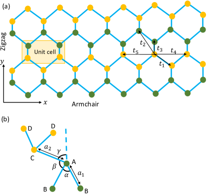
Figure 1: Schematic realization of the lattice structure of monolayer phosphorene in which the shaded circles with different colors represent atoms positioned in different planes within a single puckered layer. The shaded region shows the unit cell containing four atoms, wheras the factors $t_{1},t_{2},t_{3},t_{4},t_{5}$ characterize the five hopping parameters among the nearest neighbors in the tight binding model. (b) Schematic visualization of the bond lengths and bond angles in monolayer phosphorene.

Using the method of tight-binding model, the Hamiltonian for monolayer phosphorene with broken inversion symmetry can be described as [53, 54]

$$\mathcal{H}_{0}\left(\textbf{k}\right)=\begin{pmatrix}u_{A}+\Delta&t_{AB}\left(k\right)&t_{AD}\left(k\right)&t_{AC}\left(k\right)\\ t_{AB}\left(k\right)^{\ast}&u_{B}+\Delta&t_{AC}\left(k\right)^{\ast}&t_{AD}\left(k\right)\\ t_{AD}\left(k\right)^{\ast}&t_{AC}\left(k\right)&u_{D}-\Delta&t_{AB}\left(k\right)\\ t_{AC}\left(k\right)^{\ast}&t_{AD}\left(k\right)^{\ast}&t_{AB}\left(k\right)^{\ast}&u_{C}-\Delta\end{pmatrix},$$ (1)

with eigenvectors $\left[\psi_{A}\ \psi_{B}\ \psi_{D}\ \psi_{C}\right]^{T}$ and $u_{A}$, $u_{B}$, $u_{C}$, and $u_{D}$ are the on-site energies, which are taken as $U$, with the $A-D$ subscripts characterizing the four sublattice labels shown in Fig. 1. Moreover, $t_{AB}\left(k\right)$, $t_{AC}\left(k\right)$, and $t_{AD}\left(k\right)$ denote the coupling factors. Considering the $C_{2h}$ group symmetry of the black phosphorus lattice structure [55] and $t_{AD}\left(k\right)^{\ast}=t_{AD}\left(k\right)$, a reduced two-band Hamiltonian for monolayer phosphorene in the vicinity of the Fermi level can be obtained as [53]

$$\mathcal{H}_{0}\left(\textbf{k}\right)=\begin{pmatrix}U+t_{AD}\left(k\right)+\Delta&t_{AB}\left(k\right)+t_{AC}\left(k\right)\\ t_{AB}\left(k\right)^{\ast}+t_{AC}\left(k\right)^{\ast}&U+t_{AD}\left(k\right)-\Delta\end{pmatrix},$$ (2)

where

$$t_{AB}\left(k\right) =2t_{1}\cos\left[k_{x}a_{1}\sin\left(\alpha/2\right)\right]e^{-ik_{y}a_{1}\cos\left(\alpha/2\right)}$$

$$+2t_{3}\cos\left[k_{x}a_{1}\sin\left(\alpha/2\right)\right]e^{ik_{y}\left[a_{1}\cos\left(\alpha/2\right)+2a_{2}\cos\gamma\right]},$$ (3)

$$t_{AC}\left(k\right) =t_{2}e^{ik_{y}a_{2}\cos\beta}+t_{5}e^{-ik_{y}\left[2a_{1}\cos\left(\alpha/2\right)+a_{2}\cos\gamma\right]},$$ (4)

$$t_{AD}\left(k\right) =4t_{4}\cos\left\{k_{y}\left[a_{1}\cos\left(\alpha/2\right)+a_{2}\cos\gamma\right]\right\}$$

$$\times\cos\left[k_{x}a_{1}\sin\left(\alpha/2\right)\right],$$ (5)

where the bond length, $a_{1}=2.22\ \textrm{\AA}$ represents the distance between nearest-neighbor sites in sublattices $A$ and $B$ or $C$ and $D$ and $a_{2}=2.24\ \textrm{\AA}$ is the distance between nearest-neighbor sites in sublattices $A$ and $C$ or $B$ and $D$; the bond angles are $\alpha=96^{\circ},5^{\circ}$, $\beta=101^{\circ},9^{\circ}$, $\cos\gamma=-\cos\beta/\cos\alpha$ as shown in Fig. 1 (b), whereas $t_{1}=-1.220\ \textrm{eV}$, $t_{2}=3.665\ \textrm{eV}$, $t_{3}=-0.205\textrm{eV}$, $t_{4}=-0.105\ \textrm{eV}$, and $t_{5}=-0.055\ \textrm{eV}$, see Fig. 1 (a), are the corresponding hopping parameters for nearest-neighbor couplings [54]. Using Eq. (1), solution of the secular equation leads to the energy dispersion in the form

$$E_{\lambda}\left(k_{x},k_{y}\right)=U+t_{AD}$$

$$+\lambda\sqrt{\left(t_{AB}+t_{AC}\right)\left(t_{AB}+t_{AC}\right)^{\ast}+\Delta^{2}},$$ (6)

where $\lambda=\pm 1$ is the band index, with the positive sign showing the conduction band and negative sign characterizes the valence band. Hence, expanding the structure factors in the vicinity of $\Gamma$ point and retaining the terms up to second order in $k$, the two-band Hamiltonian of monolayer phosphorene with broken inversion symmetry within the long-wavelength approximation can be obtained as [19]

$$\mathcal{H}_{0}\left(\textbf{k}\right) =\left(u_{0}+\eta_{x}k^{2}_{x}+\eta_{y}k^{2}_{y}\right)\mathbb{1}+\left(\delta+\gamma_{x}k^{2}_{x}+\gamma_{y}k^{2}_{y}\right)\sigma_{x}$$

$$-\chi k_{y}\sigma_{y}+\sigma_{z}\Delta,$$ (7)

where $u_{0}=-0.42\ \textrm{eV}$, $\delta=0.76\ \textrm{eV}$, $\eta_{x}=0.58\ \textrm{eV}\textrm{\AA}^{2}$, $\eta_{y}=1.01\ \textrm{eV}\textrm{\AA}^{2}$, $\gamma_{x}=3.93\ \textrm{eV}\textrm{\AA}^{2}$, $\gamma_{y}=3.83\ \textrm{eV}\textrm{\AA}^{2}$, and $\chi=5.25\ \textrm{eV}\textrm{\AA}$ are the band parameters which remain the same as used in Ref. [53] and they include the contribution from the five-hopping energies of the tight-binding model for a BP sheet and its lattice geometry as shown in Fig. 1. In Eq. (II.1), $k_{x}$ and $k_{y}$ are the in-plane crystal momenta, whereas $\sigma_{x}$, $\sigma_{y}$, and $\sigma_{z}$ represent the $2\times 2$ Pauli matrices and $\mathbb{1}$ stands for the unit matrix. Moreover, $\Delta$ denotes the broken inversion symmetry induced band gap in the energy spectrum of the system. The energy dispersion of monolayer phosphorene is

$$E_{\lambda}\left(k_{x},k_{y}\right) =\in_{1}+\lambda\sqrt{\in^{2}_{2}+\Delta^{2}},$$ (8)

where we have defined: $\in_{1}\equiv u_{0}+\eta_{x}k^{2}_{x}+\eta_{y}k^{2}_{y}$, $\in_{3}\equiv\delta+\gamma_{x}k^{2}_{x}+\gamma_{y}k^{2}_{y}$, $\in_{4}\equiv\chi k_{y}$, $\in_{2}\equiv\sqrt{\in^{2}_{3}+\in^{2}_{4}}$. The first term in the right hand side of Eq. (8) makes the band structure of phosphorene highly anisotropic. The Hamiltonian in Eq. (II.1) can be diagonalized using the standard diagonalization method. Consequently, using the polar notation, normalized eigenstates of the aforementioned Hamiltonian are described as

$$\psi_{\lambda}\left(k_{x},k_{y}\right)=\frac{e^{i\textbf{k}\cdot\textbf{r}}}{\sqrt{2S}}\left(\begin{array}[]{ccc}\sqrt{1+\lambda\cos\theta_{k}}\\ \\ e^{-i\varphi_{k}}\lambda\sqrt{1-\lambda\cos\theta_{k}}\end{array}\right),$$ (9)

with $S$ being the dimensions of the system, $\tan\varphi_{k}=\frac{\in_{4}}{\in_{3}}$, and $\tan\theta_{k}=\frac{\in_{2}}{\Delta}$.
The inversion symmetry breaking in monolayer phosphorene leads to a finite Berry curvature. Such curvature in momentum space can be evaluated using Eqs. (8) and (9) in the vicinity of the $\Gamma$ point as [19]

$$\Omega_{\lambda}\left(\textbf{k}\right)=\lambda\chi\gamma_{x}k_{x}\Delta$$

$$\times\frac{\left[\left(\in_{3}-\frac{\gamma_{y}\in^{2}_{4}}{\chi^{2}}\right)\left(\in_{3}-\frac{3\gamma_{y}\in^{2}_{4}}{\chi^{2}}\right)-\in^{2}_{4}\left(1+\frac{3\gamma^{2}_{y}\in^{2}_{4}}{\chi^{4}}\right)\right]}{\left(\in^{2}_{3}+\in^{2}_{4}+\Delta^{2}\right)^{3/2}\left(\in^{2}_{3}+\in^{2}_{4}\right)}.$$ (10)

It is illustrated that the Berry curvatures of the conduction ($\lambda=+$) and valence ($\lambda=-$) bands have opposite signs and vanish in the absence of the band gap induced in the energy spectrum. The Berry curvature exhibits very interesting symmetry properties [19].

II.2 Semiclassical Dynamics of Wave Packet

We develop formalism for semiclassical dynamics of a particle in monolayer phosphorene with broken inversion symmetry. We consider a single particle that is prepared in a wave packet state having center of mass at position r with momentum k [26, 30]. The Bloch velocity of a wave packet can be described as

$$\dot{\textbf{r}}_{\lambda}=\frac{1}{\hbar}\pmb{\nabla}_{k}E_{\lambda}\left(\textbf{k}\right)-\left(\dot{\textbf{k}}\times\textbf{e}_{z}\right)\Omega_{\lambda}\left(\textbf{k}\right),$$ (11)

with

$$\hbar\dot{\textbf{k}}=\textbf{F},$$ (12)

where $\textbf{e}_{z}$ is the unit vector in the $z$-direction, the first term on the right hand side of Eq. (11) denotes the group velocity evaluated by taking the gradient of energy spectrum in momentum space and the second term describes the Berry velocity. Eq. (11) shows that the electron band velocity is periodic in crystal momentum $k$. It has been found that the effects of Berry curvature can also be determined in the semiclassical dynamics of a wave packet in a time-dependent one-dimensional (1D) optical lattice [56, 57, 58] which is defined over a 2D parameter space, composed of the one-dimensional quasimomentum and time. The Bloch oscillations of a wave packet in such a potential have been investigated in Ref. [58].
We evaluate the Bloch velocity of the wave packet in the conduction band using Eqs. (8), (II.1), and (11). As a consequence, the $x$-component of the velocity acquires the form

$$v_{x}\left(\bf{k}\right) =-\frac{4d_{1}t_{4}}{\hbar}g_{1}\left(k\right)-\frac{2d_{1}}{\hbar}\left\{4g_{2}\left(k\right)+g_{3}\left(k\right)+4g_{4}\left(k\right)\right.$$

$$\left.+4g_{5}\left(k\right)+\Delta^{2}\right\}^{-1/2}\left\{g_{6}\left(k\right)+g_{7}\left(k\right)+g_{8}\left(k\right)\right\}$$

$$+\frac{F_{y}}{\hbar}\Omega_{\lambda}\left(\textbf{k}\right),$$ (13)

and the $y$-component is

$$v_{y}\left(\bf{k}\right) =-\frac{4d_{1}t_{4}}{\hbar}g_{9}\left(k\right)-\frac{2d_{1}}{\hbar}\left\{4g_{2}\left(k\right)+g_{3}\left(k\right)+4g_{4}\left(k\right)\right.$$

$$\left.+4g_{5}\left(k\right)+\Delta^{2}\right\}^{-1/2}\left\{4g_{10}\left(k\right)+g_{11}\left(k\right)+g_{12}\left(k\right)\right.$$

$$\left.+g_{13}\left(k\right)\right\}-\frac{F_{x}}{\hbar}\Omega_{\lambda}\left(\textbf{k}\right),$$ (14)

where we have defined:

$$g_{1}\left(k\right)=\sin\left(k_{x}d_{1}\right)\cos\left(k_{y}d_{2}\right),$$

$$g_{2}\left(k\right)=\left[t^{2}_{1}+t^{2}_{3}+2t_{1}t_{3}\cos\left(2k_{y}d_{2}\right)\right]\cos^{2}\left(k_{x}d_{1}\right),$$

$$g_{3}\left(k\right)=t^{2}_{2}+t^{2}_{5}+2t_{2}t_{5}\cos\left(2k_{y}d_{2}\right),$$

$$g_{4}\left(k\right)=t_{3}\left[t_{2}\cos\left(k_{y}d_{2}\right)+t_{5}\cos\left(3k_{y}d_{2}\right)\right]\cos\left(k_{x}d_{1}\right),$$

$$g_{5}\left(k\right)=t_{1}\left(t_{2}+t_{5}\right)\cos\left(k_{x}d_{1}\right)\cos\left(k_{y}d_{2}\right),$$

$$g_{6}\left(k\right)=\left[t^{2}_{1}+t^{2}_{3}+2t_{1}t_{3}\cos\left(2k_{y}d_{2}\right)\right]\sin\left(2k_{x}d_{1}\right),$$

$$g_{7}\left(k\right)=t_{3}\left[t_{2}\cos\left(k_{y}d_{2}\right)+t_{5}\cos\left(3k_{y}d_{2}\right)\right]\sin\left(k_{x}d_{1}\right),$$

$$g_{8}\left(k\right)=t_{1}\left(t_{2}+t_{5}\right)\sin\left(k_{x}d_{1}\right)\cos\left(k_{y}d_{2}\right),$$

$$g_{9}\left(k\right)=\cos\left(k_{x}d_{1}\right)\sin\left(k_{y}d_{2}\right),$$

$$g_{10}\left(k\right)=t_{1}t_{3}\sin\left(2k_{y}d_{2}\right)\cos^{2}\left(k_{x}d_{1}\right),$$

$$g_{11}\left(k\right)=t_{2}t_{5}\sin\left(2k_{y}d_{2}\right),$$

$$g_{12}\left(k\right)=t_{3}\left[t_{2}\sin\left(k_{y}d_{2}\right)+t_{3}t_{5}\sin\left(3k_{y}d_{2}\right)\right]\cos\left(k_{x}d_{1}\right),$$

$$g_{13}\left(k\right)=t_{1}\left(t_{2}+t_{5}\right)\cos\left(k_{x}d_{1}\right)\sin\left(k_{y}d_{2}\right).$$ (15)

Eqs. (II.2) and (II.2) reveal that the Bloch velocities $v_{x}\left(\textbf{k}\right)$ and $v_{y}\left(\textbf{k}\right)$ exhibit oscillatory behaviour over the entire range of $k_{x}$ and $k_{y}$. It is illustrated that both $v_{x}\left(\textbf{k}\right)$ and $v_{y}\left(\textbf{k}\right)$ consist of group and Berry velocities which can be separated as

$$\textrm{v}_{\textbf{k}}\left(+\textbf{F}\right)+\textrm{v}_{\textbf{k}}\left(-\textbf{F}\right)=\frac{2}{\hbar}\frac{\partial E\left(\textbf{k}\right)}{\partial\textbf{k}}.$$ (16)

$$\textrm{v}_{\textbf{k}}\left(+\textbf{F}\right)-\textrm{v}_{\textbf{k}}\left(-\textbf{F}\right)=-\frac{2}{\hbar}\left(\textbf{F}\times\textbf{e}_{z}\right)\Omega\left(\textbf{k}\right).$$ (17)

This transformation is equivalent to a time-reversal operation, and it obviously removes the effects of the complex Lissajous-like figures in 2D. Interesting behaviours are exhibited by the Bloch velocity $v\left(k_{x},ky\right)$ in the Brillouin zone. In particular, the $x$-component of the group velocity, $v_{x}\left(k_{x},ky\right)$, vanishes at $k_{x}=0,\ k_{y}\neq 0$ as is clear from Eq. (16), whereas the $y$-component, $v_{y}\left(k_{x},ky\right)$, remains finite. Likewise, $v_{y}\left(k_{x},ky\right)$ vanishes at $k_{y}=0,\ k_{x}\neq 0$, $v_{x}\left(k_{x},ky\right)$ remains finite. Further, $v_{x}\left(k_{x},ky\right)$ changes its sign by changing the sign of $k_{x}$, whereas $v_{y}\left(k_{x},ky\right)$ changes its sign with $k_{y}$. Moreover, the group velocity is affected by the band gap opened in the energy spectrum due to the broken inversion symmetry, however, it remains finite even if the aforementioned symmetry is retained. In contrast, Berry velocity depends on the inversion symmetry breaking which becomes zero if the system preserves the inversion symmetry. The Berry velocity in Eq. (17), $v_{j}\left(k_{x},ky\right)$ with $j=x,y$, exhibits the following symmetry properties: (i) The Berry velocity shows mirror reflection symmetry $k_{y}\leftrightarrow-k_{y}$, i.e., $v_{j}\left(k_{x},-k_{y}\right)=v_{j}\left(k_{x},k_{y}\right)$. (ii) It remains finite in a crystal system with broken inversion symmetry, i.e., a crystal lattice with inversion symmetry requires $v_{j}\left(\textbf{k}\right)=v_{j}\left(-\textbf{k}\right)=0$. (iii) It shows the character of an odd function in momentum space, i.e., $v_{j}\left(-k_{x},k_{y}\right)=-v_{j}\left(k_{x},k_{y}\right)$, reflecting time-reversal symmetry of the system. (iv) It changes sign when the direction of the applied force is reversed.

III Results and Discussion on Bloch Dynamics

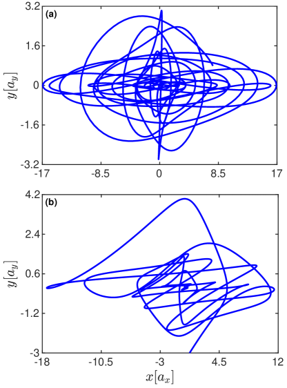
Figure 2: Lissajous-like figure for a wave packet in inversion symmetry broken monolayer phosphorene using the ratio: (a) $F_{x}:F_{y}=2F_{0}:12F_{0}$ and (b) $F_{x}:F_{y}=12F_{0}:2F_{0}$ with $F_{0}=\delta/a_{x}$. Parameters used in the numerical simulations are: $a_{x}\equiv a_{1}=3.32\textrm{\AA}$; $a_{y}\equiv a_{2}=4.38\textrm{\AA}$; $\Delta=\delta$ and other parameters are the same as given in the text.

In this section, we present the results on Bloch oscillations in monolayer phosphorene with broken inversion symmetry. For analyzing the remarkable feature of dimensionality, we plot the real-space trajectories of the Bloch oscillations in Fig. 2 which reveals Lissajous-like oscillations. It has been shown that 1D Bloch oscillations in the presence of separable potentials are simply superposed along the $x$ and $y$-axes. The wave packet dynamics exhibits periodic behaviour along $k_{i}$ with periods $T_{j}=h/|F_{j}|a$ for an arbitrary force $F=\left(F_{x},F_{y}\right)$. The resulting dynamics depends on the ratio $F_{x}:F_{y}$. For nonseparable potentials, similar dynamical behavior can be expected when the applied force is weak and Landau-Zener tunneling is negligibly small [48, Witthaut-NJP.6:41].

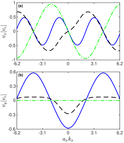
Figure 3: Group velocity of charge carrier in inversion symmetry broken monolayer phosphorene in units of $v_{c}$, with $v_{c}=\chi/\hbar$ being the characteristic velocity, versus the crystal momentum $k_{x}$. Panel (a) shows the group velocity in the $x$-direction, whereas (b) in the $y$-direction. In each panel, the blue solid curve is used for $k_{y}d_{2}=\frac{\pi}{2}$, black dashed curve for $k_{y}d_{2}=\frac{\pi}{4}$, and green dash-dotted curve for $k_{y}d_{2}=\pi$. The parameters used in the numerical simulations are the same as used for Fig. 2.

The real-space Lissajous-like figures describe complicated two-dimensional oscillations, which are bounded by $x_{j}\propto v_{j}T_{j}$, see Fig. 2. Note that we have adopted a scheme in which the ratio $F_{x}:F_{y}$ has been made large, where the Bloch electron covers a large area of the Brillouin zone during a single Bloch oscillation. It is obvious that the Lissajous-like figure is approximately bounded by the Bloch oscillation lengths, and so it makes the effects of Berry curvature ambiguous within the bounded region.
This trajectory can be changed significantly by the Berry curvature, if we wait until the wave packet drifts outside the bounded region. As a consequence, only the net Berry curvature encountered along a path will be measured in experiments. Information regarding the distribution of Berry curvature in momentum space will be lost, in particular, whether its sign changes. Moreover, an additional drift in the position of wave packet may occur in 2D, independent of the Berry curvature, if the wave packet does not start at high symmetry points such as the zone center $k_{0}=(0,0)$ [59, 60]. Hence, merely the observation of a transverse drift in the position of wave packet is not a conclusive evidence of a finite Berry curvature.
To better understand the Bloch dynamics in monolayer phosphorene, the group velocity of the Bloch electron as a function of crystal momentum $k_{x}$ is plotted in Fig. 3. This figure shows that the group velocity of the Bloch electron is well pronounced in the Brillouin zone that strongly depends on the initial momentum $k_{y}$ as is obvious from comparison of the blue solid, black dashed, and green dash-dotted curves. In particular, the change in initial crystal momentum $k_{y}$ leads to the change of phase and amplitude of oscillations. Comparison of panels (a) and (b) shows that the group velocities $v_{x}$ and $v_{y}$ exhibit different dynamical behaviour, where the latter vanishes at $k_{y}=\pi/d_{2}$. Further, the oscillation frequency and amplitude of oscillations of the two components are also very different.

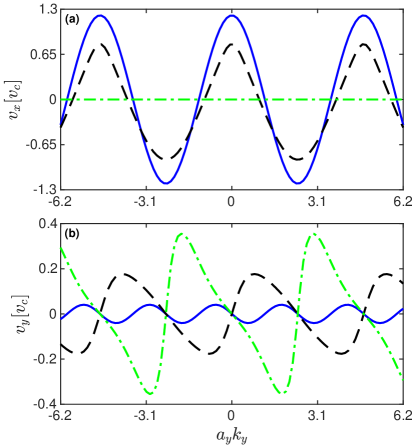
Figure 4: Group velocity of charge carrier in inversion symmetry broken monolayer phosphorene versus the crystal momentum $k_{y}$. Panel (a) shows the group velocity in the $x$-direction, whereas (b) in the $y$-direction. In each panel, the blue solid curve is used for $k_{x}d_{1}=\frac{\pi}{2}$, black dashed curve for $k_{x}d_{1}=\frac{\pi}{4}$, and green dash-dotted curve for $k_{x}d_{1}=\pi$ and other parameters remain the same as used for Fig. 2.

For more insight, we show the group velocity of the Bloch electron as a function of the crystal momentum $k_{y}$ in Fig. 4 for different values of the initial momentum $k_{x}$. It mimics the behaviour of group velocity as shown in Fig. 3. However in this case, the group velocity $v_{x}$ vanishes at $k_{x}=\pi/d_{1}$, see panel (a), where $v_{y}$ remains finite, see panel (b). Likewise, comparison of Figs. 3 and 4 reveals that the oscillation frequency and amplitude of oscillations of the group velocities are different as a function of $k_{x}$ and $k_{y}$, in particular, the oscillation frequency of $v_{y}$ is large when it is analyzed as a function of the crystal momentum $k_{y}$, see Figs. 3 (b) and 4 (b).

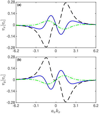
Figure 5: Berry velocity of charge carrier in inversion symmetry broken monolayer phosphorene versus the crystal momentum $k_{x}$. Panel (a) shows the Berry velocity in the $x$-direction, whereas (b) in the $y$-direction. In each panel, the blue solid curve is used for $k_{y}d_{2}=\frac{\pi}{2}$, black dashed curve for $k_{y}d_{2}=\frac{\pi}{4}$, and green dash-dotted curve for $k_{y}d_{2}=\pi$. Other parameters used in the numerical simulations are the same as used for Fig. 2.

Moreover, we show the Berry velocity as a function of crystal momentum $k_{x}$ in Fig. 5 for different values of the initial crystal momentum $k_{y}$. Analysis of this figure shows that the Berry velocity reflects the aforementioned symmetry properties. In particular, comparison of the blue solid, black dashed, and green dash-dotted curves in both panels (a) and (b) shows that the $x$- and $y$-components of the Berry velocity changes significantly by changing the initial crystal momentum $k_{y}$, where the change in amplitude and phase of oscillations can be seen. Further, comparison of panels (a) and (b) shows that the $x$- and $y$-components of the Berry velocity oscillate with phase difference of $\pi$. Interestingly, both components of the Berry velocity vanish at $k_{x}=0$ which are also negligibly small in the regions, $a_{x}k_{x}<-5$ and $a_{x}k_{x}>5$ and well pronounced in the region, $-5<a_{x}k_{x}>5$.

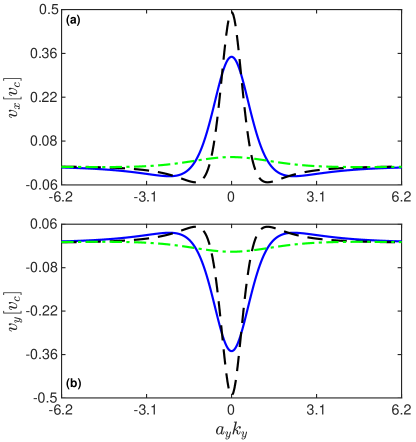
Figure 6: Berry velocity of charge carrier in inversion symmetry broken monolayer phosphorene versus the crystal momentum $k_{y}$. Panel (a) shows the Berry velocity in the $x$-direction, whereas (b) in the $y$-direction. In each panel, the blue solid curve is used for $k_{x}d_{1}=\frac{\pi}{2}$, black dashed curve for $k_{x}d_{1}=\frac{\pi}{4}$, and green dash-dotted curve for $k_{x}d_{1}=\pi$. Other parameters used in the numerical simulations are the same as used for Fig. 2.

For further understanding, the Berry velocity as a function of crystal momentum $k_{y}$ is shown in Fig. 6 for different values of the initial crystal momentum $k_{x}$. In this case, the Berry velocity exhibits interesting dynamical behaviour. In particular, a single peak around $k_{y}\approx 0$ appears in contrast to the former case when the Berry velocity is plotted as a function of $k_{x}$ where two peaks are obtained on the left and right of $k_{x}=0$ with opposite phases. Moreover, the Berry velocity vanishes in the regions, $a_{y}k_{y}\ll 0$ and $a_{y}k_{y}\gg 0$.

III.1 Bloch dynamics in an in-plane electric field along $x$-axis

In this case, the electric field is applied in the $x$-direction, i.e., $E=E_{x}$, hence $E_{y}=0$. As a consequence, $k_{y}(t)=k_{y}=\textrm{constant}$ and $k_{x}(t)=k_{x}(0)+\frac{eE_{x}}{\hbar}t$ that sweeps the entire Brillouin zone. After reaching the right end point $k_{x}=\pi/a_{x}$ electron is Bragg-reflected and continues from the left end point $k_{x}=-\pi/a_{x}$.

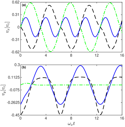
Figure 7: Bloch velocity as a function of time for monolayer phosphorene with $\omega_{x}=\frac{eE_{x}d_{1}}{\hbar}$. Panel (a) shows the Berry velocity in the $x$-direction, whereas (b) in the $y$-direction. In each panel, the blue solid curve is used for $k_{y}d_{2}=\frac{\pi}{2}$, black dashed curve for $k_{y}d_{2}=\frac{\pi}{4}$, and green dash-dotted curve for $k_{y}d_{2}=\pi$. Other parameters used in the numerical simulations are the same as used for Fig. 2.

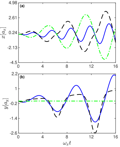
Figure 8: Real space trajectories of Bloch particle as a function of time for monolayer phosphorene for: (a) $x$-component, (b) $y$-component, where in each panel, the blue solid curve is used for $k_{y}d_{2}=\frac{\pi}{2}$, black dashed curve for $k_{y}d_{2}=\frac{\pi}{4}$, and green dash-dotted curve for $k_{y}d_{2}=\pi$. Other parameters used in the numerical simulations are the same as used for Fig. 2.

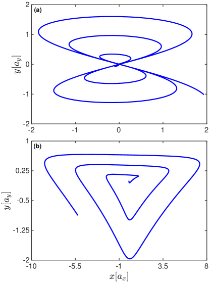
Figure 9: Lissajous-like figure of Bloch particle for monolayer phosphorene: (a) for $k_{y}d_{2}=\frac{\pi}{2}$, (b) for $k_{y}d_{2}=\frac{\pi}{4}$. Other parameters used in the numerical simulations are the same as used for Fig. 2.

As a consequence, the Bloch velocity is affected significantly by applying an in-plane electric field, which oscillates with oscillation frequency $\omega_{x}=\frac{eE_{x}d_{1}}{\hbar}$ showing its periodic character, i.e., $v_{j}\left(t+T\right)=v_{j}\left(t\right)$ with $T=\frac{2\pi}{\omega_{x}}$ being the time period of the motion. It is shown that $v_{y}\left(t\right)$ is modified strongly even if the electric field is applied in the $x$-direction because the energy dispersion couples the $x$- and $y$-components of the crystal momentum. In addition, it is obvious that for increasing value of $k_{y}$, the wave packet begins to wind the Brillouin zone in two different directions with angular frequency $\omega_{x}$. In Fig. 7, we show the Bloch velocity $v_{x}$ as a function of time with oscillation $\omega_{x}$ under the influence of an in-plane electric field applied in the $x$-direction. Fig. 7 (a) reveals that the amplitude and phase of oscillations are modified considerably by changing the initial crystal momentum $k_{y}$, see the blue solid, black dashed, and green dash-dotted curves in panel (a). Similar features of $v_{y}$ can be seen in Fig. 7 (b). In addition, comparison of panels (a) and (b) reveals different dynamical behavior of the Bloch electron in the $x$- and $y$-directions. In particular, the $x$-component of the Bloch velocity oscillates with large frequency compared to the $y$-component. Moreover, the $y$-component of the Bloch velocity vanishes for $k_{y}=\pi/d_{2}$. For further analysis, the real space trajectories of the Bloch dynamics as a function of time are shown in Fig. 8. This figure also reveals oscillatory behaviour of the Bloch dynamics in real space, depending on the initial crystal momentum $k_{y}$ as is obvious from comparison of the blue solid, black dashed, and green dash-dotted curves in panels (a) and (b), where the change in oscillation frequency and amplitude is obvious. Interestingly, the amplitude of oscillation increases with the increase in time. Moreover, we plot the real-space trajectories of the Bloch oscillations in Fig. 9 for two different values of the initial $k_{y}$ momentum which exhibits Lissajous-like oscillations. It is obvious that with increasing value of $k_{y}$, wave packet starts to wind Brillouin zone in two different directions with angular frequency $\omega_{x}$. Comparison of panels (a) and (b) reveals strong dependence of the dynamics on the initial crystal momentum $k_{y}$.

III.2 Bloch dynamics in an in-plane electric field along $y$-axis

Here we consider the case when the electric field is applied in the $y$-direction, i.e., $E=E_{y}$, hence $E_{x}=0$. In this case, the semiclassical dynamical equation shows that $k_{x}(t)=k_{x}=\textrm{constant}$ and $k_{y}(t)=k_{y}(0)+\frac{eE_{y}}{\hbar}t$. Hence, the Bloch velocity is affected significantly by applying an in-plane electric field in the $y$-direction, which oscillates with oscillation frequency $\omega_{y}=\frac{eE_{y}d_{2}}{\hbar}$ showing its periodic character, i.e., $v_{j}\left(t+T\right)=v_{j}\left(t\right)$ with $T=\frac{2\pi}{\omega_{y}}$ being the time period of the motion.

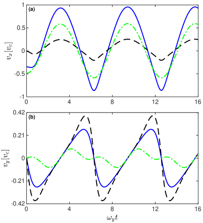
Figure 10: Bloch velocity as a function of time for monolayer phosphorene with $\omega_{y}=\frac{eE_{y}d_{2}}{\hbar}$. Panel (a) shows the Berry velocity in the $x$-direction, whereas (b) in the $y$-direction. In each panel, the blue solid curve is used for $k_{x}d_{1}=\frac{\pi}{2}$, black dashed curve for $k_{x}d_{1}=\frac{\pi}{4}$, and green dash-dotted curve for $k_{x}d_{1}=\pi$. Other parameters used in the numerical simulations are the same as used for Fig. 2.

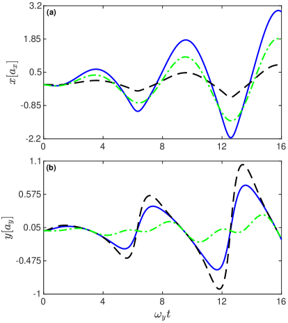
Figure 11: Real space trajectories of Bloch particle as a function of time for monolayer phosphorene for: (a) $x$-component, (b) $y$-component, where in each panel, the blue solid curve is used for $k_{x}d_{1}=\frac{\pi}{2}$, black dashed curve for $k_{x}d_{1}=\frac{\pi}{4}$, and green dash-dotted curve for $k_{x}d_{1}=\pi$. Other parameters used in the numerical simulations are the same as used for Fig. 2.

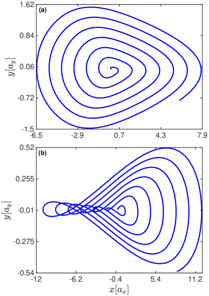
Figure 12: Lissajous-like figure of Bloch particle for monolayer phosphorene: (a) for $k_{x}d_{1}=\frac{\pi}{2}$, (b) for $k_{x}d_{1}=\frac{\pi}{4}$. Other parameters used in the numerical simulations are the same as used for Fig. 2.

In Fig. 10, we show the Bloch velocity as a function of time in monolayer phosphorene with broken inversion symmetry in an in-plane electric field E applied in the $y$-direction, using $k_{x}d_{1}=\frac{\pi}{2}$, see blue solid curves, $k_{x}d_{1}=\frac{\pi}{4}$, see black dashed curves, and $k_{x}d_{1}=\pi$, green dash-dotted curves in both panels (a) and (b). Comparison of panels (a) and (b) reveals that the wave packet undergoes pronounced oscillatory motion in monolayer phosphorene under the influence of an in-plane electric field. In addition, Fig. 10 (a) shows that the wave packet exhibits finite Bloch velocity in the $x$-direction even when the electric field is applied in the $y$-direction. Interestingly, comparison of panels (a) and (b) reveals that $v_{x}\left(t\right)$ and $v_{y}\left(t\right)$ perform out of phase oscillations with different amplitudes. Moreover, comparison of Figs. 7 and 10 shows that the Bloch velocity exhibits different dynamical behavior under the influence of applied in-plane electric field in the $x$- and $y$-directions. To realize the real space dynamics, we show the real space trajectories in Fig. 11 using the same set of parameters as used for Fig. 10. This figure reveals pronounced oscillatory behavior of the system dynamics. Comparison of the blue solid, black dashed, and green dash-dotted curves in both panels (a) and (b) reveals that the Bloch dynamics is significantly affected by the initial momentum $k_{x}$. Likewise, comparison of panels (a) and (b) shows that the $x$- and $y$-components of the Bloch dynamics exhibits different dynamical behaviour. For further understanding, we plot the real-space trajectories of the Bloch oscillations in Fig. 12 for two different values of the initial $k_{x}$ momentum which exhibits Lissajous-like oscillations. Comparison of panels (a) and (b) reveals the strong dependence of Bloch dynamics on the initial momentum $k_{x}$. Moreover, comparison of Figs. 9 and 12 shows the difference in dynamical behavior of Bloch dynamics under the influence of applied in-plane electric field in the $x$- and $y$-directions.

III.3 Effect of spin-orbit interaction on Bloch dynamics

In this section, the effect of spin-orbit interaction (SOI) on the Bloch dynamics in monolayer phosphorene with broken inversion symmetry is investigated. This study is expected to be useful in understanding the spin-dependent electronic properties that may pave the way for potential applications of phosphorene in spintronic devices. Interesting effects are induced by the spin-orbit interaction in phosphorene [9, 12, 13]. The details of spin-orbit interaction in phosphorene can be found in [19, 18]. Here we focus merely on its impact on Bloch oscillations. In this paper, the effects of spin-orbit interaction are incorporated considering the intrinsic spin–orbit coupling within the framework of Kane–Mele model which takes into account appropriately the effects of spin up and spin down states as used in phosphorene [61, 18, 19], borophene [62], lattice system [63], graphene [64], and, silicene [65].

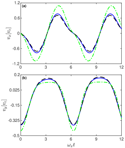
Figure 13: Bloch velocity as a function of time for monolayer phosphorene, illustrating the effect of spin-orbit interaction. Panel (a) shows the Berry velocity in the $x$-direction, whereas (b) in the $y$-direction. In each panel, the blue solid curve is used for $k_{y}d_{2}=\frac{\pi}{2}$, black dashed curve for $k_{y}d_{2}=\frac{\pi}{4}$, and green dash-dotted curve for $k_{y}d_{2}=\pi$. The parameters used are: $\Delta=\delta,\ \Delta_{SO}=0.6\delta,\ \Delta_{z}=2\delta$ and other parameters used in the numerical simulations are the same as used for Fig. 2.

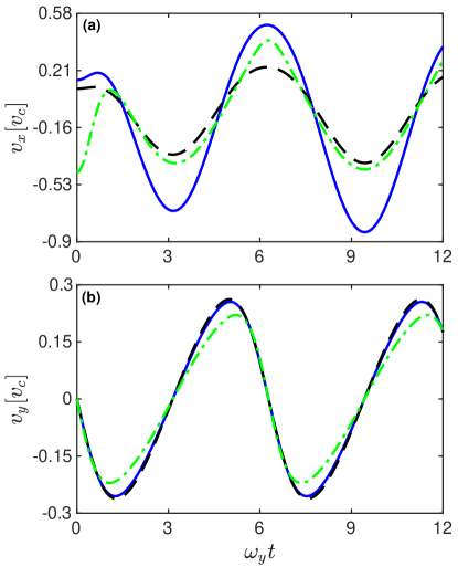
Figure 14: Bloch velocity as a function of time for monolayer phosphorene, illustrating the effect of spin-orbit interaction. Panel (a) shows the Berry velocity in the $x$-direction, whereas (b) in the $y$-direction. In each panel, the blue solid curve is used for $k_{x}d_{1}=\frac{\pi}{2}$, black dashed curve for $k_{x}d_{1}=\frac{\pi}{4}$, and green dash-dotted curve for $k_{x}d_{1}=\pi$. The parameters used in the numerical simulations are the same as used for Fig. 12.

The Hamiltonian of monolayer phosphorene with broken inversion symmetry under the influence of intrinsic spin-orbit interaction can be described as

$$\mathcal{H}\left(\textbf{k}\right) =\mathcal{H}_{0}\left(\textbf{k}\right)+\mathcal{H}_{SOI}\left(\textbf{k}\right),$$ (18)

where $\mathcal{H}_{0}\left(\textbf{k}\right)$ is given in Eq. (2), whereas $\mathcal{H}_{SOI}\left(\textbf{k}\right)=\Delta_{z}\sigma_{z}-s_{z}\Delta_{SOI}\sigma_{z}$ characterizes the Kane-Mele Hamiltonian, denoting the intrinsic spin-orbit interaction (SOI) and induces the SOI gap, $\Delta_{SOI}$, in the energy spectrum of the system. The factor, $\Delta_{z}=lE_{z}$ with the length scale $l=2.26\textrm{\AA}$, takes into account the effects of electric field $E_{z}$ applied perpendicular to the sample. Likewise, $s_{z}=\pm$ stands for the spin direction such that $s_{z}=+$ represents spin up and $s_{z}=-$ characterizes the spin down state. The Hamiltonian in Eq. (18) can be diagonalized using the standard diagonalization method. Using the obtained eigenenergies, one can readily evaluate the velocities of the Bloch electron. In Fig. 13, we show the Bloch velocity as a function of time using $\Delta=\delta,\ \Delta_{SOI}=0.6\delta,\ \Delta_{z}=2\delta$, where panel (a) represents the $x$-component and (b) the $y$-component under the influence of an in-plane electric field in the $x$-direction. In each panel, the green dash-dotted curve shows the Bloch dynamics without spin-orbit coupling, the blue solid curve for spin up, whereas the black dashed curve for spin down states. Comparison of the blue solid, black dashed, and green dash-dotted curves in both panels (a) and (b) shows that the spin-orbit interaction remarkably changes the Bloch oscillations, depending on the strength of interaction. Moreover, comparison of panels (a) and (b) reveals that the effect of SOI is more pronounced on the $x$-component of the Bloch velocity compared to the $y$-component. In addition, comparison of the blue solid and black dashed curves shows that the response of the spin up and spin states are different. In Fig. 14, we show the effect of spin-orbit coupling on the velocity of Bloch electron in monolayer phosphorene with broken inversion symmetry when the in-plane electric is applied in the $y$-direction. Comparison of the blue solid, black dashed, and green dash-dotted curves in both panels (a) and (b) shows that the spin-orbit interaction changes the Bloch oscillations considerably, depending on the strength of interaction. Moreover, comparison of panels (a) and (b) reveals that the effect of SOI is more pronounced on the $x$-component of the Bloch velocity compared to the $y$-component. Further comparison of the blue solid and black dashed curves shows that the response of the spin up and spin states are different. Furthermore, comparison of Figs. 13 and 14 shows that the SOI affects differently when the in-plane electric field is applied in the $x$- and $y$-directions.

III.4 Confined-deconfined state transition

In this section, we study the effect of in-plane electric and transverse magnetic fields on the Bloch dynamics in monolayer phosphorene which essentially leads to a transition from confined to deconfined states and vice versa that strongly depend on the relative strength of the fields.

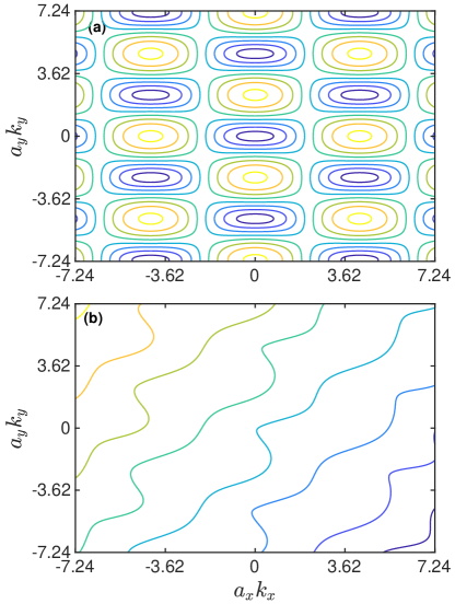
Figure 15: Confined-to-deconfined transition by analyzing the trajectories of $H\left(k_{x},k_{y}\right)$: (a) $eE=0.1F_{0}$, $B=6T$; (b) $eE=6F_{0}$, $B=0.1T$, which are contours in momentum space, depending on the strength of electric and magnetic. Other parameters remain the same as used for Fig. 2.

In this case, the wave packet dynamics in conduction band is determined using the semiclassical dynamical equation

$$\hbar\dot{\textbf{k}}=e\textbf{E}+e\textbf{v}\times\textbf{B},$$ (19)

where E is the applied electric field and B is the magnetic field. Solving Eqs. (11), (II.2), (II.2), and (19), we can study the Bloch dynamics in a monolayer phosphorene with broken inversion symmetry. The position $\textbf{r}(t)=\int^{t}_{0}\textbf{v}(t^{\prime})dt^{\prime}$ can be determined by integrating the equation of motion:

$$\hbar\left[\textbf{k}(t)-\textbf{k}(0)\right]=e\textbf{E}t+e\textbf{r}(t)\times\textbf{B}.$$ (20)

In the confined (B-dominated) regime, the drift velocity $\textbf{v}_{d}=\textbf{r}(t)/t|_{nT}$ is given by

$$\textbf{v}_{d}=\textbf{E}\times\textbf{B}/B^{2}.$$ (21)

In the transition to deconfined (E-dominated) regime, the drift velocity abruptly drops to zero. Interesting dynamics appears in an applied transverse magnetic field, where dynamical phase transition to one-frequency oscillation occurs. As a consequence, the system exhibits complex dynamics at the transition. It is shown that under the influence of in-plane electric and transverse magnetic fields, two distinct types of cyclotron orbits are formed depending on the relative strength of E and B: (i) when magnetic field dominates the in-plane electric field, confined orbits are formed which reside within the Brillouin zone and characterized by one Bloch frequency, (ii) however, de-confined orbits are generated when E-field dominates B-field which extend over infinitely many Brillouin zones and are described by two or more frequencies. It is illustrated that confinement in $k$-space means deconfinement in $r$-space, and vice versa. Here the equations of motion can be determined in terms of a Hamiltonian function as [71]

$$\dot{k}_{x}=\frac{\partial H\left(k_{x},k_{y}\right)}{\partial k_{y}},\quad\dot{k}_{y}=-\frac{\partial H\left(k_{x},k_{y}\right)}{\partial k_{x}},$$ (22)

where the Hamiltonian function is defined as

$$H\left(k_{x},k_{y}\right)=\frac{eB}{\hbar^{2}}E\left(\textbf{k}\right)+\frac{e}{\hbar}\left|\textbf{E}\times\textbf{k}\right|,$$ (23)

where $E\left(\textbf{k}\right)$ denotes the energy dispersion and E characterizes the applied electric field. The trajectories of wave packet appear as contours of $H\left(k_{x},k_{y}\right)$ in momentum space. The effects of electric and magnetic fields on the Bloch dynamics are incorporated appropriately using Eq. (23). Note that the trajectories are confined orbits in the Brillouin zone with single frequency in the regime, $E<vB$, whereas de-confined orbits are formed which are extended over infinitely many Brillouin zones with two or more frequencies when $E>vB$. To highlight this effect, the contours of the Hamiltonian function in Eq. (23) are plotted as a function of crystal momenta, $k_{x}$ and $k_{y}$, in Fig. 15, illustrating the confinement and deconfinement of orbits which depend on the relative strength of the electric and magnetic fields. This figure shows that the orbits are confined in the regime $E<vB$, see Fig. 15(a), however the orbits exhibit de-confined behaviour when the strength of electric field is greater than the magnetic field, i.e., $E>vB$, see Fig. 15(b).

IV Conclusions

In summary, we have studied Bloch dynamics in monolayer phosphorene with broken inversion symmetry within the framework of semiclassical theory. We have shown that the Bloch velocity of a wave packet exhibits pronounced oscillations in both real and momentum spaces, called Bloch oscillations. It has been found that an applied in-plane electric field modifies significantly the Bloch oscillations in the system, depending on its magnitude and direction. Dynamical transition is driven by an applied magnetic field, leading to a complex dynamics at the transition point. In the presence of both external in-plane electric and transverse magnetic fields, the system undergoes a dynamical transition from confined to de-confined state and vice versa, tuned by the relative strength of the applied fields which was also observed in a moiré flat band system [71]. In this case, two distinct types of cyclotron orbits are formed, depending on the relative strength of E and B: (i) when magnetic field dominates the in-plane electric field, confined orbits are formed which reside within the Brillouin zone and characterized by a single Bloch frequency, (ii) however, de-confined orbits are generated when E-field dominates B-field which extend over infinitely many Brillouin zones and are described by two or more frequencies. The equations of motion can be derived by defining a Hamiltonian function $H\left(k_{x},k_{y}\right)$ with trajectories in the form of contours in momentum space. It has been shown that the confinement of orbits depends on the relative strength of electric and magnetic fields such that the orbits are confined when the strength of magnetic field is greater than the electric field, i.e., $vB>E$, which however become de-confined for $vB<E$. It is illustrated that the Bloch dynamics in monolayer phosphorene with broken inversion symmetry presents a dynamical scenario that differs from the Bloch oscillations in moiré flat band system [71]. For instance, in the present study, we have focussed on the investigation of Bloch velocity composed of Berry and group velocities, whereas in the latter system we have studied the group velocity only with focus on the effect of twist angle with preserved inversion symmetry of the system. Due to the difference in models, the results of the two systems are very different. However, in both systems we have studied the Bloch oscillations under the influence of external fields such as in-plane electric and transverse magnetic fields, where in both systems the wave packets exhibit pronounced Bloch oscillations and the system undergoes a dynamical transition. The experimental measurement of Bloch oscillations in monolayer phosphorene with broken inversion symmetry is expected to be possible using the techniques developed for observing oscillations on the surface of black phosphorus using a gate electric field [69], transport measurements of phosphorene-hexagonal BN (hBN) heterostructures with one-dimensional edge contacts [70], and time-resolved band gap emission spectroscopy [72].

Data availability statement

Data sharing is not applicable to this article, as it describes entirely theoretical research work.

References

- [1] A. S. Rodin, A. Carvalho, and A. H. Castro Neto, Phys. Rev. Lett. 112, 176801 (2014).
- [2] T. Low et al., Phys. Rev. Lett. 113, 106802 (2014).
- [3] J. Qiao, X. Kong, Z.-X. Hu, F. Yang, W. Ji, Nat. Commun. 5, 4475 (2014).
- [4] F. Xia, H. Wang and Y. Jia, Nat. Commun. 5, 4458 (2014).
- [5] X. Wang et al., Nat. Nanotechnol. 10, 517 (2015).
- [6] Y. Lee et al., Nano Lett. 20, 559 (2020).
- [7] L. Li et al., Nat. Nanotechnol. 9, 372 (2014).
- [8] W. Lu et al., Nano Res. 7, 853 (2014).
- [9] M. Kurpas, M. Gmitra, and J. Fabian, Phys. Rev. B 94, 155423 (2016).
- [10] F. Sattari, Mater. Sci. Eng. B 278, 115625 (2022).
- [11] X. Luo, X. Feng, Y. Liu, and J. Guo, Opt. Express 28, 9089 (2020).
- [12] S. M. Farzaneh, S. Rakheja, Phys. Rev. B 100, 245429 (2019).
- [13] Z. S. Popović, J. M. Kurdestany, and S. Satpathy, Phys. Rev. B 92, 035135 (2015).
- [14] Tony Low, Yongjin Jiang, and Francisco Guinea, Phys. Rev. B 92, 235447 (2015).
- [15] R. Fei and L. Yang, Nano Lett. 14, 2884 (2014).
- [16] S. Hu et al., Phys. Rev. B 97, 045209 (2018).
- [17] M. Elahi, K. Khaliji, S. M. Tabatabaei, M. Pourfath, and R. Asgari, Phys. Rev. B 91, 115412 (2015).
- [18] Rifat Sultana and Abdullah Yar, J. Phys. Chem. Solids 176, 111257 (2023).
- [19] Abdullah Yar and Rifat Sultana, J. Phys.: Condens. Matter 35, 165701 (2023).
- [20] A. K. Tareen et al., Prog. Solid. State Ch. 65, 100336 (2022).
- [21] X. Ling, H. Wang, S. Huang, and M. S. Dresselhaus, Proc. Natl. Acad. Sci. U.S.A. 112, 4523 (2015).
- [22] H. O. H. Churchill and P. Jarillo-Herrero, Nat. Nanotechnol. 9, 330 (2014).
- [23] H. Liu, Y. Du, Y. Deng, P. D. Ye, Chem. Soc. Rev. 44, 2732 (2015).
- [24] F. Bloch, Z. Phys. 52, 555 (1929).
- [25] C. Zener, Proc. R. Soc. London, Ser. A 145, 523 (1934).
- [26] N.W. Ashcroft and N. D. Mermin, Solid State Physics (Saunders, Philadelphia, 1976).
- [27] Z. Pagel et al., Phys. Rev. A 102, 053312 (2020).
- [28] A. R. Kolovsky and E. N. Bulgakov, Phys. Rev. A 87, 033602 (2013).
- [29] J. Feldmann et al., Phys. Rev. B 46, 7252(R) (1992).
- [30] M. B. Dahan, E. Peik, J. Reichel, Y. Castin, and C. Salomon, Phys. Rev. Lett. 76, 4508 (1996).
- [31] B. P. Anderson and M. A. Kasevich, Science 282, 1686 (1998).
- [32] R. Battesti et al., Phys. Rev. Lett. 92, 253001 (2004).
- [33] Y. Zhang et al., Optica 4, 571 (2017).
- [34] O. Morsch, J. H. Müller, M. Cristiani, D. Ciampini, and E. Arimondo, Phys. Rev. Lett. 87, 140402 (2001).
- [35] T. Pertsch, P. Dannberg, W. Elflein, A. Bräuer, and F. Lederer, Phys. Rev. Lett. 83, 4752 (1999).
- [36] R. Morandotti, U. Peschel, J. S. Aitchison, H. S. Eisenberg, and Y. Silberberg, Phys. Rev. Lett. 83, 4756 (1999).
- [37] R. Sapienza et al., Phys. Rev. Lett. 91, 263902 (2003).
- [38] H. Trompeter et al., Phys. Rev. Lett. 96, 023901 (2006).
- [39] H. Trompeter et al., Phys. Rev. Lett. 96, 053903 (2006).
- [40] A. Block et al., Nat. Commun. 5, 3843 (2014).
- [41] J. Höller and A. Alexandradinata, Phys. Rev. B 98, 024310 (2018).
- [42] A. Nenciu, G. Nenciu, Phys. Lett. A 78, 101 (1980).
- [43] P. Cladé et al., Phys. Rev. Lett. 96, 033001 (2006).
- [44] G. Roati et al., Phys. Rev. Lett. 92, 230402 (2004).
- [45] G. Ferrari, N. Poli, F. Sorrentino, and G. M. Tino, Phys. Rev. Lett. 97, 060402 (2006).
- [46] J. Stockhofe, and P. Schmelcher, Phys. Rev. A 91, 023606 (2015).
- [47] D. Witthaut, F. Keck, H. J. Korsch and S. Mossmann, New J. Phys. 6, 41 (2004).
- [48] A. R. Kolovsky and H. J. Korsch, Phys. Rev. A 67, 063601 (2003).
- [49] H. M. Price and N. R. Cooper, Phys. Rev. A 85, 033620 (2012).
- [50] Yan-Qi Wang and Xiong-Jun Liu, Phys. Rev. A 94, 031603(R) (2016).
- [51] L. Masi et al., Phys. Rev. Lett. 127, 020601 (2021).
- [52] W. Zhang et al., Nat. Commun. 13, 2392 (2022).
- [53] J. M. Pereira Jr. and M. I. Katsnelson, Phys. Rev. B 92, 075437 (2015).
- [54] A. N. Rudenko and M. I. Katsnelson, Phys. Rev. B 89, 201408(R) (2014).
- [55] M. Ezawa, New J. Phys. 16, 115004 (2014).
- [56] D. Xiao, M.-C. Chang, and Q. Niu, Rev. Mod. Phys. 82, 1959 (2010).
- [57] T. Kitagawa, E. Berg, M. Rudner, and E. Demler, Phys. Rev. B 82, 235114 (2010).
- [58] G. Pettini and M. Modugno, Phys. Rev. A 83, 013619 (2011).
- [59] S. Mossmann, A. Schulze, D. Witthaut, and H. J. Korsch, J. Phys. A: Math. Gen. 38, 3381 (2005).
- [60] J. M. Zhang and W. M. Liu, Phys. Rev. A 82, 025602 (2010).
- [61] H. Rezania, M. Abdi and B. Astinchap, Eur. Phys. J. Plus 137, 18 (2022).
- [62] A. Yar, G. Bahadar, Ikramullah, and K. Sabeeh, Phys. Lett. A 429, 127916 (2022).
- [63] F. D. M. Haldane, Phys. Rev. Lett. 61, 2015 (1988).
- [64] C. L. Kane and E. J. Mele, Phys. Rev. Lett. 95, 226801 (2005).
- [65] V. Vargiamidis, P. Vasilopoulos, and G.-Q. Hai, J. Phys.: Condens. Matter 26, 345303 (2014).
- [66] J. Balakrishnan, G. K. W. Koon, M. Jaiswal, A. H. Castro Neto and B. Özyilmaz, Nat. Phys. 9, 284 (2013).
- [67] A. Ferreira, Tatiana G. Rappoport, M. A. Cazalilla, and A. H. Castro Neto, Phys. Rev. Lett. 112, 066601 (2014).
- [68] A. H. Castro Neto and F. Guinea Phys. Rev. Lett. 103, 026804 (2009).
- [69] L. Li et al., Nat. Nanotech. 10, 608 (2015).
- [70] N. Gillgren et al., 2D Mater. 2, 011001 (2015).
- [71] A. Yar, B. Sarwar, S. B. A. Shah, and K. Sabeeh, Phys. Lett. A 478, 128899 (2023).
- [72] L. Li et al., Opt. Express 26, 23844 (2018).