Adversaries with Limited Information in the Friedkin–Johnsen Model

Abstract

In recent years, online social networks have been the target of adversaries who seek to introduce discord into societies, to undermine democracies and to destabilize communities. Often the goal is not to favor a certain side of a conflict but to increase disagreement and polarization. To get a mathematical understanding of such attacks, researchers use opinion-formation models from sociology, such as the Friedkin–Johnsen model, and formally study how much discord the adversary can produce when altering the opinions for only a small set of users. In this line of work, it is commonly assumed that the adversary has full knowledge about the network topology and the opinions of all users. However, the latter assumption is often unrealistic in practice, where user opinions are not available or simply difficult to estimate accurately.

To address this concern, we raise the following question: Can an attacker sow discord in a social network, even when only the network topology is known? We answer this question affirmatively. We present approximation algorithms for detecting a small set of users who are highly influential for the disagreement and polarization in the network. We show that when the adversary radicalizes these users and if the initial disagreement/polarization in the network is not very high, then our method gives a constant-factor approximation on the setting when the user opinions are known. To find the set of influential users, we provide a novel approximation algorithm for a variant of MaxCut in graphs with positive and negative edge weights. We experimentally evaluate our methods, which have access only to the network topology, and we find that they have similar performance as methods that have access to the network topology and all user opinions. We further present an $\mathbf{NP}$-hardness proof, which was left as an open question by Chen and Racz [IEEE Transactions on Network Science and Engineering, 2021].

1 Introduction

Online social networks have become an integral part of modern societies and are used by billions of people on a daily basis. In addition to connecting people with their friends and family, online social networks facilitate societal deliberation and play an important role in forming the political will in modern democracies.

However, during recent years we have had ample evidence of malicious actors performing attacks on social networks so as to destabilize communities, sow disagreement, and increase polarization. For instance, a report issued by the United States Senate finds that Russian “trolls monitored societal divisions and were poised to pounce when new events provoked societal discord” and that this “campaign [was] designed to sow discord in American politics and society” [38]. Another report found that both left- and right-leaning audiences were targeted by these trolls [16]. Similarly, a recent analysis regarding the Iranian disinformation claimed that “the main goal is to control public opinion—pitting groups against each other and tarnishing the reputations of activists and protesters” [28].

The study of how such attacks influence societies can be facilitated by models of opinion dynamics, which study the mechanisms for individuals to form their opinions in social networks. Relevant research questions have been investigated in different disciplines, e.g., psychology, social sciences, and economics [12, 29, 3, 43, 34]. A popular model for studying such questions in computer science [25, 36, 45, 9, 2, 44, 41] is the Friedkin–Johnsen model (FJ) [19], which is a generalization of the DeGroot model [15].

To understand the power of an adversarial actor over the opinion-formation process in a social network, there are two popular measures of discord: disagreement and polarization; for the rest of the paper, we use the word discord to refer to either disagreement or polarization; see Section 2 for the formal definitions.

Previous works studied the increase of discord that can be inflicted by a malicious attacker who can change the opinions of a small number of users. As an example, Chen and Racz [13] showed that even simple heuristics, such as changing the opinions of centrists, can lead to a significant increase of the disagreement in the network. They also presented theoretical bounds, which were later extended by Gaitonde, Kleinberg and Tardos [21].

Crucially, the previous methods assume that the attacker has access to the network topology as well as the opinions of all users. However, the latter assumption is rather impractical: user opinions are either not available or difficult to estimate accurately. On the other hand, obtaining the network topology is more feasible, as networks often provide access to the follower and interaction graphs.

As knowledge of all user opinions appears unrealistic, we raise the following question: Can attackers sow a significant amount of discord in a social network, even when only the network topology is known? In other words, we consider a setting with limited information in which the adversary has to pick a small set of users, without knowing the user opinions in the network.

Our Contributions. Our main contributions are as follows. First, we provide a formal connection between the settings of full (all user opinions are known) and limited information (the user opinions are unknown). Informally, we show that if the variance of user opinions in the network is not very high (and some other mild technical assumptions), then an adversary who radicalizes the users who are highly influential for the network obtains a $\mathcal{O}(1)$-approximation for the setting when all user opinions are known. Thus, we answer the above question affirmatively from a theoretical point of view.

Second, we implement our algorithms and evaluate them on real-world datasets. Our experiments show that for maximizing disagreement, our algorithms, which use only topology information, outperform simple baselines and have similar performance as existing algorithms that have full information. Therefore, we also answer the above question affirmatively in practice.

Third, we provide constant-factor approximation algorithms for identifying $\Omega(n)$ users who are highly influential for the discord in the network, where $n$ is the number of users in the network. We derive analytically the concept of highly-influential users for network discord and we formalize an associated computational task (Section 3.1). Our formulation allows us to obtain insights into which users drive the disagreement and the polarization in social networks. We also show that this problem is $\mathbf{NP}$-hard, which solves an open problem by Chen and Racz [13].

Fourth, we show that to find the users who are influential on the discord, we have to solve a version of cardinality constrained MaxCut in graphs with both positive and negative edge weights. For this problem, we present the first constant-factor approximation algorithm when the number of users to radicalize is $\Omega(n)$. Here the main technical challenge arises from the presence of negative edges, which imply that the problem is non-submodular and which rule out using averaging arguments that are often used to analyze such algorithms [6, A.3.2]. Hence, existing algorithms do not extend to our more general case and we prove analogous results for graphs with positive and negative edge weights. In addition, our $\mathbf{NP}$-hardness proof provides a further connection between maximizing the disagreement and MaxCut.

We discuss some of the ethical aspects of our findings regarding the power of a malicious adversary who has access to the topology of a social network in the conclusion (Section 5).

Related work. A recently emerging and popular topic in the area of graph mining is to study optimization problems based on FJ opinion dynamics. Papers considered minimizing disagreement and polarization indices [36], maximizing opinions [25], changes of the network topology [45, 9] or changes of the susceptibility to persuasion [2]. Xu et al. [44] show how to efficiently estimate quantities such as the polarization and disagreement indices. Our paper is also conceptually related to the topic of maximizing influence in social networks, pioneered by Kempe, Kleinberg and Tardos [30]; the influence-maximization model has recently been combined with opinion-formation processes [41]. Furthermore, many extensions of the classic FJ model have been proposed [5, 37].

Most related to our work are the papers by Chen and Racz [13] and by Gaitonde, Kleinberg and Tardos [21], who consider adversaries who plan network attacks. They provide upper bounds when an adversary can take over $k$ nodes in the network, and they present heuristics for maximizing disagreement in the setting with full information. A practical consideration of this model has motivated us to study settings with limited information. While their adversary can change the opinions of $k$ nodes to either $0$ or $1$, in this paper we are mainly concerned with adversaries which can change the opinions of $k$ nodes to $1$; we consider the adversary’s actions as “radicalizing $k$ nodes.” Our setting is applicable in scenarios when opinions near opinion value $0$ ($1$) correspond to non-radicalized (radicalized) views.

Our algorithm for MaxCut in graphs with positive and negative edge weights is based on the SDP-rounding techniques by Goemans and Williamson [26] for MaxCut, and by Frieze and Jerrum [20] for MaxBisection. While their results assume that the matrix $\mathbf{A}$ in Problem (3.2) is the Laplacian of a graph with positive edge weights, our result in Theorem 3.3 applies to more general matrices, albeit with worse approximation ratios. Currently, the best approximation algorithm for MaxBisection is by Austrin et al. [7]. Ageev and Sviridenko [4] gives LP-based algorithms for versions of MaxCut with given sizes of parts, Feige and Langberg [18] extended this work to an SDP-based algorithm; but their techniques appear to be inherently limited to positive edge-weight graphs and cannot be extended to our more general setting of Problem (3.2).

2 Preliminaries

Let $G=(V,E,w)$ be an undirected weighted graph representing a social network. The edge-weight function $w\colon E\rightarrow\mathbb{R}_{>0}$ models the strengths of user interactions. We write $\left\lvert V\right\rvert=n$ for the number of nodes, and use $N(u)$ to denote the set of neighbors of node $u\in V$, i.e., $N(u)=\{v:(u,v)\in E\}$. We let $\mathbf{D}$ be the $n\times n$ diagonal matrix with $\mathbf{D}_{v,v}=\sum_{u\in N(v)}w(u,v)$ and define the weighted adjacency matrix $\mathbf{W}$ by $\mathbf{W}_{u,v}=w(u,v)$. The Laplacian of the graph $G$ is given by $\mathbf{L}=\mathbf{D}-\mathbf{W}$.

In the Friedkin–Johnsen opinion-dynamics model (FJ) [19], each node $u\in V$ corresponds to a person who has an innate opinion and an expressed opinion. For each node $u$, the innate opinion $s_{u}\in[0,1]$ is fixed over time and kept private; the expressed opinion $z_{u}^{(t)}\in[0,1]$ is publicly known and it changes over time $t\in\mathbb{N}$ due to peer pressure. Initially, $z_{u}^{(0)}=s_{u}$ for all users $u\in V$. At each time $t>0$, all users $u\in V$ update their expressed opinion $z_{u}^{(t)}$ as the weighted average of their innate opinion and the expressed opinions of their neighbors, as follows:

$$z_{u}^{(t)}=\frac{s_{u}+\sum_{v\in N(u)}w_{uv}z_{v}^{(t-1)}}{1+\sum_{v\in N(u)}w_{uv}}.$$ (2.1)

We write $\mathbf{z}^{(t)}=(z_{1}^{(t)},\dots,z_{n}^{(t)})$ to denote the vector of expressed opinions at time $t$. Similarly, we set $\mathbf{s}=(s_{1},\dots,s_{n})$ for the innate opinions. In the limit $t\to\infty$, the expressed opinions reach the equilibrium $\mathbf{z}=\lim_{t\to\infty}\mathbf{z}^{(t)}=(\mathbf{I}+\mathbf{L})^{-1}\mathbf{s}$.

We study the behavior of the following two discord measures in the FJ opinion-dynamics model:

Disagreement index ([36]) $\mathcal{D}_{G,\mathbf{s}}=\sum_{(u,v)\in E}w_{u,v}(z_{u}-z_{v})^{2}=\mathbf{s}^{\intercal}{\mathcal{D}}(\mathbf{L})\,\mathbf{s}$, where ${\mathcal{D}}(\mathbf{L})\,=(\mathbf{L}+\mathbf{I})^{-1}\mathbf{L}(\mathbf{L}+\mathbf{I})^{-1}$, and

Polarization index ([35, 36]) $\mathcal{P}_{G,\mathbf{s}}=\sum_{u\in V}(z_{u}-\bar{\mathbf{z}})^{2}=\mathbf{s}^{\intercal}{\mathcal{P}}(\mathbf{L})\,\mathbf{s}$, where $\bar{\mathbf{z}}=\frac{1}{n}\sum_{u\in V}z_{u}$ is the average user opinion and ${\mathcal{P}}(\mathbf{L})\,=(\mathbf{I}+\mathbf{L})^{-1}(\mathbf{I}-\frac{\mathbf{1}\mathbf{1}^{\intercal}}{n})(\mathbf{I}+\mathbf{L})^{-1}$.

Note that the disagreement index measures the discord along the edges of the network, i.e., it measures how much interacting nodes disagree. The polarization index measures the overall discord in the network by considering the variance of the opinions.

We note that the matrices ${\mathcal{D}}(\mathbf{L})\,$ and ${\mathcal{P}}(\mathbf{L})\,$ may have positive and negative off-diagonal entries and it is not clear whether they are diagonally dominant; this is in contrast to graph Laplacians that have exclusively non-positive off-diagonal entries and are diagonally dominant. Having positive and negative entries will be one of the challenges we need to overcome later. The following lemma presents some additional properties.

Lemma 2.1.

Let $\mathbf{A}\in\{{\mathcal{D}}(\mathbf{L})\,,{\mathcal{P}}(\mathbf{L})\,\}$. Then $\mathbf{A}$ is positive semidefinite and satisfies $\mathbf{A}\mathbf{1}=\mathbf{0}$, where $\mathbf{1}$ is the all-ones vector and $\mathbf{0}$ is the all-zeros vector.

While we consider opinions in the interval $[0,1]$, for the $\mathbf{NP}$-hardness results presented later, for technical reasons, it will be useful to consider opinions in the interval $[-1,1]$. In Appendix B.1, we show that the solutions of optimization problems are maintained under scaling, which implies that our $\mathbf{NP}$-hardness results and our $\mathcal{O}(1)$-approximation algorithm also apply for opinions in the $[0,1]$ interval.

We present all omitted proofs in Appendix B.

3 Problem definition and algorithms

We start by defining the problem of maximizing the discord when $k$ user opinions can be radicalized, i.e., when for $k$ users the innate opinions can be changed from their current value $\mathbf{s}_{0}(u)$ to the extreme value $1$. This problem is of practical relevance when opinions close to $0$ correspond to non-radicalized opinions (“covid-19 vaccines are generally safe”) and opinions close to $1$ correspond to radicalized opinions (“covid-19 vaccines are harmful”). Then an adversary can radicalize $k$ people by setting their opinion to $1$, for instance, by supplying them with fake news or by hacking their social network accounts. Formally, our problem is stated as follows.

Problem 3.1.

Let $\mathbf{A}\in\{{\mathcal{D}}(\mathbf{L})\,,{\mathcal{P}}(\mathbf{L})\,\}$. Consider an undirected weighted graph $G=(V,E,w)$, and innate opinions $\mathbf{s}_{0}\in[0,1]^{n}$. We want to maximize the discord where we can radicalize the innate opinions of $k$ users. In matrix notation, the problem is as follows:

$$\max_{\mathbf{s}} \mathbf{s}^{\intercal}\mathbf{A}\mathbf{s},$$ (3.1)

such that $$\lVert\mathbf{s}-\mathbf{s}_{0}\rVert_{0}=k,\text{ and}$$

$$\mathbf{s}(u)\in\{\mathbf{s}_{0}(u),1\}\text{ for all }u\in V.$$

Note that if we set $\mathbf{A}={\mathcal{D}}(\mathbf{L})\,$ the problem is to maximize the disagreement in the network. If we set $\mathbf{A}={\mathcal{P}}(\mathbf{L})\,$ we seek to maximize the polarization.

Further observe that for Problem (3.1), the algorithm obtains as input the graph $G$ and the vector of innate opinions $\mathbf{s}_{0}$. Therefore, we view this formulation as the setting with full information.

Central to our paper is the idea that the algorithm has access to the topology of the graph $G$, but it does not have access to the initial innate opinions $\mathbf{s}_{0}$. As discussed in the introduction, we believe that this scenario is of higher practical relevance, as it seems infeasible for an attacker to gather the opinions of millions of users in online social networks. On the other hand, assuming access to the network topology, i.e., the graph $G$, appears more feasible because networks, such as Twitter, make this information publicly available.

Our approach for maximizing the discord, even when we have limited information, i.e., we only have access to the graph topology, has two steps:

1. Detect a small set $S$ of $k$ users who are highly influential for the discord in the network.

2. Change the innate opinions for the users in the set $S$ to $1$ and leave all other opinions unchanged.

In the rest of this section, we will describe our overall approach for finding a set of $k$ influential users on the discord (Section 3.1) and then we will discuss approximation algorithms (Section 3.2) and heuristics (Section 3.3) for this task. Then, we prove computational hardness (Section 3.4).

3.1 Finding influential users on the discord

Next, we describe the implementation of Step (1) discussed above. In other words, we wish to find a set $S$ of $k$ users who are highly influential for the discord in the network.

To form an intuition about highly-influential users for the network discord in the absence of information about user innate opinions, we consider scenarios of non-controversial topics. Since the topics are non-controversial, we expect most users to have opinions near a consensus opinion $c$. In such scenarios, an adversary who aims to radicalize $k$ users so as to maximize the network discord, will seek to find a set $S$ of $k$ users and set $\mathbf{s}_{0}(u)=1$, for $u\in S$, so as to maximize the discord $\mathbf{s}^{\intercal}\mathbf{A}\mathbf{s}$, where $\mathbf{A}\in\{{\mathcal{D}}(\mathbf{L})\,,{\mathcal{P}}(\mathbf{L})\,\}$.

Since we assume most opinions to be near consensus $c$, it seems natural that the concrete value of $c\in[0,1]$ has no big effect on the choice of the users picked by the adversary (see also Theorem 3.2 which formalizes that this intuition is correct). Hence, we consider $c=0$ and study the idealized version of the problem, where $\mathbf{s}_{0}(u)=0$ for all users $u$ in the network. In this case, the adversary will need to solve the following optimization problem:

$$\begin{aligned} \max_{\mathbf{s}}\quad&\mathbf{s}^{\intercal}\mathbf{A}\mathbf{s},\\ \text{such that}\quad&\lVert\mathbf{s}\rVert_{0}=k,\text{ and}\\ &\mathbf{s}\in[0,1]^{n}.\end{aligned}$$ (3.2)

The result of the above optimization problem is a vector $\mathbf{s}$ that has $k$ non-zero entries, all of which are equal to $1$. Thus, we can view the set $S=\{u\mid\mathbf{s}_{0}(u)=1\}$ as a set of users who are highly influential for the discord in the network.

We provide a constant-factor approximation algorithm for this problem in Theorem 3.3. We also show that the problem is $\mathbf{NP}$-hard in Theorem 3.9 when $\mathbf{A}={\mathcal{D}}(\mathbf{L})\,$, which answers an open question by Chen and Racz [13].

Relationship between the limited and full information settings. At first glance, it may not be obvious why a solution for Problem (3.2) with limited information implies a good solution for Problem (3.1) with full information. However, we will show that this is indeed the case when there is little initial discord in the network; we believe this is the most interesting setting for attackers who wish to increase the discord.

Slightly more formally (see Theorem 3.2 for details), we show the following. If initially all innate opinions are close to the average opinion $c$ and some mild assumptions hold, then an $\mathcal{O}(1)$-approximate solution for Problem 3.2 (when only the network topology is known) implies an $\mathcal{O}(1)$-approximate solution for Problem 3.1 (when full information including user opinions are known).

Before stating the theorem, we define some additional notation. For a set of users $X\subseteq V$, we write $\mathbf{s}_{X}$ to denote the vector of innate opinions when we radicalize the users in $X$, i.e., $\mathbf{s}_{X}\in[0,1]^{n}$ satisfies $\mathbf{s}_{X}(u)=1$ if $u\in X$ and $\mathbf{s}_{X}(u)=\mathbf{s}_{0}(u)$ if $u\not\in X$. Furthermore, given $X$ and a vector $\mathbf{v}$, we write $\mathbf{v}_{|X}$ to denote the restriction of $v$ to the entries in $X$, i.e., $\mathbf{v}_{|X}(u)=\mathbf{v}(u)$ if $u\in X$ and $\mathbf{v}_{|X}(u)=0$ if $u\not\in X$. We discuss our technical assumptions after the theorem.

Theorem 3.2.

Let $\mathbf{A}\in\{{\mathcal{D}}(\mathbf{L})\,,{\mathcal{P}}(\mathbf{L})\,\}$. Let $c\in[0,1)$ and $\hat{\mathbf{r}}\in[-c,1-c]^{n}$ be such that $\mathbf{s}_{0}=c\mathbf{1}+\hat{\mathbf{r}}$. Let $\gamma_{1},\gamma_{2},\gamma_{3}\in(0,1)$ be parameters. Furthermore, assume that for all sets $X\subseteq V$ with $\left\lvert X\right\rvert=k$ it holds that:

1. $(\mathbf{s}_{X}-\mathbf{s}_{0})^{\intercal}\mathbf{A}\mathbf{s}_{0}\geq-\gamma_{1}\mathbf{s}_{0}^{\intercal}\mathbf{A}\mathbf{s}_{0}$,

2. $\hat{\mathbf{r}}_{|X}^{\intercal}\mathbf{A}\hat{\mathbf{r}}_{|X}\leq\gamma_{2}\mathbf{s}_{0}^{\intercal}\mathbf{A}\mathbf{s}_{0}$, and

3. $\left\lvert\hat{\mathbf{r}}_{|X}^{\intercal}\mathbf{A}\mathbf{1}_{|X}\right\rvert\leq\gamma_{3}\mathbf{s}_{0}^{\intercal}\mathbf{A}\mathbf{s}_{0}$.

Suppose we have access to a $\beta$-approximation algorithm for Problem (3.2) with limited information. Then we can compute a solution for Problem (3.1) with full information with approximation ratio $\frac{1}{4}\min\{\beta,\frac{1-2\gamma_{1}-2(1-c)\gamma_{3}}{1+2(1-c)\gamma_{3}+\gamma_{2}}\}$, even if we only have access to the graph topology (but not the user opinions).

One may think of $c$ as the average innate opinion and $\hat{\mathbf{r}}$ as the vector that indicates how much each innate opinion deviates from $c$. Indeed, for topics that initially have little discord, one may assume that most entries in $\hat{\mathbf{r}}$ are small.

The intuitive interpretation of the technical conditions from the theorem is as follows. Condition (1) corresponds to the assumption that no matter which $k$ users the adversary radicalizes, the discord will not drop by more than a $\gamma_{1}$-fraction. This rules out some unrealistic scenarios in which, for example, all but $k$ users have initial innate opinion $1$ and one could subsequently remove the entire discord by radicalizing the remaining $k$ users. Conditions (2) and (3) are of similar nature and essentially state that if only $k$ users have the opinions given by $\hat{\mathbf{r}}$ and all other users have opinion $0$, then the discord in the network is significantly smaller than the initial discord when all $n$ users have the opinions in $\mathbf{s}_{0}$.

Note that when $k\ll n$, it is reasonable to assume that $\gamma_{1}$, $\gamma_{2}$, $\gamma_{3}$ are upper-bounded by a small constant, say $\frac{1}{5}$. In this case the theorem states that if we have a $\beta$-approximation algorithm for the setting with limited information then we obtain an $\mathcal{O}(\beta)$-approximation algorithm for the setting with full information, even though we only use the network topology but not the innate opinions.

3.2 $\alpha$-Balanced MaxCut

In this section, we study the $\alpha$-Balanced-MaxCut problem for which we present a constant-factor approximation algorithm. This algorithm allows us to solve Problem (3.2) (maximizing discord with limited information) approximately. Combined with Theorem 3.2 above, this implies that (under some assumptions) adversaries with limited information only perform a constant factor worse than those with full information (see Corollary 3.5 below).

In the $\alpha$-Balanced-MaxCut problem, the goal is to partition a set of nodes into two sides such that one side contains an $\alpha$-fraction of the nodes and the cut is maximized. Formally, we are given a positive semidefinite matrix $\mathbf{A}\in\mathbb{R}^{n\times n}$ and a parameter $\alpha\in[0,1]$. The goal is to solve the following problem:

$$\max_{\mathbf{x}}\quad\frac{1}{4} \mathbf{x}^{\intercal}\mathbf{A}\mathbf{x},$$ (3.3)

such that $$\lVert\mathbf{x}+\mathbf{1}\rVert_{0}=\alpha n,\text{ and}$$

$$\mathbf{x}\in[-1,1]^{n}.$$

Note that the optimal solution vector $\mathbf{x}$ takes values in $\{-1,1\}$ (since the objective function is convex, as $\mathbf{A}$ is positive semidefinite) and thus it partitions the set $V$ into two sets $S=\{u\colon\mathbf{x}_{u}=1\}$ and $\bar{S}=\{u\colon\mathbf{x}_{u}=-1\}$. The first constraint ensures $\left\lvert S\right\rvert=\alpha n$ and $\left\lvert\bar{S}\right\rvert=(1-\alpha)n$, i.e., one side contains an $\alpha$-fraction of the nodes and the other side contains a $(1-\alpha)$-fraction. If $\mathbf{A}$ is the Laplacian of a graph and $\alpha=\frac{1}{2}$, this is the classic MaxBisection problem [20]. Hence, we will sometimes refer to $\mathbf{x}$ and the corresponding partition $(S,\bar{S})$ as a cut and to $\mathbf{x}^{\intercal}\mathbf{A}\mathbf{x}$ as the cut value.

Our main result for Problem (3.3) is as follows.

Theorem 3.3.

Suppose $\alpha\in[0,1]$ is a constant and $\mathbf{A}$ is a symmetric, positive semidefinite matrix with $\mathbf{1}^{\intercal}\mathbf{A}=\mathbf{0}^{\intercal}$. Then for any $0<\epsilon<1$, there exists a randomized polynomial time algorithm that with probability at least $1-\epsilon$, outputs a solution for the $\alpha$-Balanced-MaxCut (Problem (3.3)) with approximation ratio presented in Figure 1. The algorithm runs in time $O(1/\epsilon\log(1/\epsilon)poly(n))$.

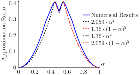
Figure 1: The approximation ratio from Theorem 3.3 as function of $\alpha$. We present numerical approximation ratio results compared with a piece-wise quadratic function defined by the formulas: $2.059\alpha^{2}$ for $0<\alpha<0.448$, $1.36(1-\alpha)^{2}$ for $0.448\leq\alpha<0.5$, $1.36\alpha^{2}$ for $0.5\leq\alpha<0.552$, and $2.059(1-\alpha)^{2}$ for $0.552\leq\alpha<1$.

In Figure 1 we visualize the approximation ratios for different values of $\alpha$. In particular, observe that for any constant $\alpha\in(0,1]$, our approximation ratio is $\Omega(1)$ and that for most values of $\alpha$ it performs within at a least a factor of $10$ of the optimal solution. Furthermore, for $\alpha$ close to $0.5$, our approximation is better than $\frac{1}{3}$.

Before we discuss Theorem 3.3 in more detail, we first present two corollaries. First, we observe that the theorem implies that we obtain a constant-factor approximation algorithm for maximizing the discord with limited information (Problem (3.2)).

Corollary 3.4.

Let $k=\alpha n$. If $\alpha\in[0,1]$ is a constant, there exists an $\mathcal{O}(1)$-approximation algorithm for Problem (3.2) with limited information that runs in polynomial time.

Proof.

Observe that a solution for Problem (3.3) implies a solution for Problem (3.2) as follows: Suppose in Problem (3.3) we set $\mathbf{A}=4{\mathcal{D}}(\mathbf{L})\,$ or $\mathbf{A}=4{\mathcal{P}}(\mathbf{L})\,$ and $\alpha=\frac{k}{n}$ to obtain a solution $\mathbf{x}$. Now we define a solution $\mathbf{s}$ for Problem (3.3) by setting $\mathbf{s}(u)=1$ if $\mathbf{x}(u)=1$ and $\mathbf{s}(u)=0$ if $\mathbf{x}(u)=-1$. Observe that $\lVert\mathbf{s}\rVert_{0}=k$ as desired. Since the last step can be viewed as rescaling opinions from $[-1,1]$ to $[0,1]$, the objective function values of $\mathbf{x}^{\intercal}\mathbf{A}\mathbf{x}$ and $\mathbf{s}^{\intercal}\mathbf{A}\mathbf{s}$ only differ by a factor of $4$ (see Appendix B.1). ∎

Second, observe that by combining Theorems 3.2 and Corollary 3.4, we immediately obtain the following result for solving the setting with full information, even when we only have access to the network topology.

Corollary 3.5.

Suppose $\alpha\in[0,1]$ is a constant and the conditions of Theorem 3.2 hold with $\gamma_{1},\gamma_{2},\gamma_{3}\leq\frac{1}{5}$. Then there exists a polynomial time algorithm for Problem (3.1) with full information that has approximation ratio $\mathcal{O}(1)$ and only uses the graph topology (but not the user opinions).

Next, let us discuss Theorem 3.3 in more detail.

The theorem generalizes previous results and its approximation ratios are only a small constant factor worse than classic results [26, 20, 27]. In particular, the previous results assumed that $\mathbf{A}$ is the Laplacian of a graph with positive edge weights, and thus $\mathbf{A}$ has the structure that all off-diagonal entries are nonpositive. In contrast, in our result we do require the latter assumption and allow for positive off-diagonal entries, which appear, for instance, in graphs with negative edge weights. Indeed, this is the case for the matrices ${\mathcal{D}}(\mathbf{L})\,$ and ${\mathcal{P}}(\mathbf{L})\,$ from Section 2, which may have positive off-diagonal entries. Therefore, our generalized theorem is necessary to maximize the discord in Problem (3.2).

Furthermore, we note that to apply Theorem 3.3 on graphs with both positive and negative edge weights, we have to assume that their Laplacian is positive semidefinite. This assumption cannot be dropped, as pointed out by Williamson and Shmoys [42, Section 6.3]. This is crucial since, while for graphs with positive edge weights the Laplacian is always positive semidefinite, this is not generally true for graphs with negative edge weights. However, this assumption holds in our use cases due to Lemma 2.1.

In the theorem we require $\alpha\in[0,1]$ to be a constant and thus $k=\Omega(n)$. While this is somewhat undesirable, there are underlying technical reasons for it: the SDP-based approach by Frieze and Jerrum [20] also has this requirement; LP-based algorithms which work for $k=o(n)$ (as shown, for instance, by Ageev and Sviridenko [4]) do not generalize to the setting in which the matrices are not graph Laplacians; the same is the case for the SDP-based approach by Feige and Langberg [18].

Algorithm. Our algorithm is based on solving the SDP relaxation of Problem (3.3) and applying random hyperplane rounding [26], followed by a greedy step in which we adjust the sizes of the sets $S$ and $\bar{S}$. Later, we will see that our main technical challenge will be to prove that the greedy adjustment step still works in our more general setting.

To obtain our SDP relaxation of Problem (3.3), we observe that by the convexity of the objective function we can assume that $\mathbf{s}\in\{-1,1\}^{n}$ (see Appendix B.4) and thus, we can rewrite the constraint $\lVert\mathbf{x}+\mathbf{1}\rVert_{0}=\alpha n$  as  $2\sum_{i<j}^{n}\mathbf{x}_{i}\mathbf{x}_{j}=n^{2}(1-2\alpha)^{2}-n$.

Now the semidefinite relaxation of Problem (3.3) becomes:

$$\begin{aligned} \max_{\mathbf{v}_{1},\dots,\mathbf{v}_{n}}\quad&\frac{1}{4}\sum_{ij}\mathbf{A}_{ij}\mathbf{v}_{i}^{\intercal}\mathbf{v}_{j},\\ \text{such that}\quad&\sum_{i<j}\mathbf{v}_{i}^{\intercal}\mathbf{v}_{j}=\frac{1}{2}n^{2}(1-2\alpha)^{2}-\frac{n}{2},\text{ and}\\ &\mathbf{v}_{i}\in\mathbb{R}^{n},\quad\quad\|\mathbf{v}_{i}\|_{2}=1.\end{aligned}$$ (3.4)

1 Solve the SDP in Equation (3.4) with solution $\mathbf{v}_{1},\dots,\mathbf{v}_{n}$

2 for $\kappa=\mathcal{O}(1/\epsilon\log(1/\epsilon))$ times do

3      Sample vector $\mathbf{r}$ with each entry $\sim{\mathcal{N}}(0,1)$

4      Set $S=\{i:\langle\mathbf{v}_{i},\mathbf{r}\rangle\geq 0\}$ and $\bar{S}=V\setminus S$

5      Set $\bar{\mathbf{x}}_{i}=1$ if $i\in S$ and $\bar{\mathbf{x}}_{i}=-1$ if $i\in\bar{S}$

6      if $\left\lvert S\right\rvert>\alpha n$ then

7          greedily move elements from $S$ to $\bar{S}$ until $\left\lvert S\right\rvert=\alpha n$

8           if $\left\lvert S\right\rvert<\alpha n$ then

9               greedily move elements from $\bar{S}$ to $S$ until $\left\lvert S\right\rvert=\alpha n$

               

                 // In each step, move the element that decreases the value of the objective function the least

10               

11                return best solution over all trials

Algorithm 1 SDP-based relaxation followed by iterative local improvement

Our approach for solving Problem (3.3) is shown as Algorithm 1. For simplicity, we assume that $\alpha\leq\frac{1}{2}$; for $\alpha>\frac{1}{2}$ we can run the algorithm with $\alpha^{\prime}=1-\alpha\leq\frac{1}{2}$ and obtain the desirable result.

Analysis. Our analysis has two parts. The first part is the hyperplane rounding of the SDP solution; it follows the techniques of Goemans and Williamson [26] and Frieze and Jerrum [20]. The next lemma summarizes the first part of the analysis.

Lemma 3.6 ([26, 42, 20]).

The expected cut of $(S,\bar{S})$ is at least $\frac{2}{\pi}\,\mathbf{OPT}$ and $\mathbb{E}[\left\lvert S\right\rvert\left\lvert\bar{S}\right\rvert]\geq 0.878\cdot\alpha(1-\alpha)n^{2}$, where $\mathbf{OPT}$ is the optimal solution for $\alpha$-Balanced-MaxCut.

The second part of the analysis is novel and considers the greedy procedure that ensures that $S$ contains $k$ elements. When $\mathbf{A}$ is the Laplacian of a graph with nonnegative edge weights, an averaging argument (see, e.g.,  [6, A.3.2]) implies that there exists $u\in S$ such that we can move $u$ from $S$ to $\bar{S}$ and the cut value drops by a factor of at most $1/\left\lvert S\right\rvert$. However, for more general matrices $\mathbf{A}$ this may not hold, e.g., when $\mathbf{A}$ is the Laplacian of a signed graph with negative edge weights or when $\mathbf{A}$ is the matrix that corresponds to the disagreement index, as in Problem (3.2). We also illustrate this in Appendix B.5. However, we show that in our setting there always exists a node in $S$ such that if we move $u$ from $S$ to $\bar{S}$ then the cut value drops by a factor of at most $2/\left\lvert S\right\rvert$.

Lemma 3.7.

Suppose that $\mathbf{A}$ is a symmetric, positive semidefinite matrix with $\mathbf{1}^{\intercal}\mathbf{A}=\mathbf{0}^{\intercal}$ and let $\bar{\mathbf{x}}\in\{-1,1\}^{n}$. Set $M=\frac{1}{4}\bar{\mathbf{x}}^{\intercal}\mathbf{A}\bar{\mathbf{x}}$ and $S=\{i\in\{1,\ldots,n\}\mid\bar{\mathbf{x}}_{i}=1\}$. Then there exists $i\in S$ such that, by modifying $\bar{x}_{i}$ to be $-1$, $M$ decreases at most $\frac{2M}{\left\lvert S\right\rvert}$.

Proof.

We prove the lemma by contradiction. Suppose there does not exist such $i\in S$ and let $\mathbf{e}_{i}\in\mathbb{R}^{n}$ denote the vector whose $i$-th entry is $1$ and all other entries are $0$s. Then for any $i$, it holds

$$M-\frac{1}{4}(\bar{\mathbf{x}}-2\mathbf{e}_{i})^{\intercal}\mathbf{A}(\bar{\mathbf{x}}-2\mathbf{e}_{i})>\frac{2M}{\left\lvert S\right\rvert}.$$

Expanding and simplifying the formula, we get

$$\mathbf{e}_{i}^{\intercal}\mathbf{A}\bar{\mathbf{x}}>\frac{2M}{\left\lvert S\right\rvert}+\mathbf{e}_{i}^{\intercal}\mathbf{A}\mathbf{e}_{i},$$

for all $i\in S$. Summing this inequality over all $i\in S$, we obtain

$$\sum_{i\in S}\mathbf{e}_{i}^{\intercal}\mathbf{A}\bar{\mathbf{x}}>2M+\sum_{i\in S}\mathbf{e}_{i}^{\intercal}\mathbf{A}\mathbf{e}_{i}.$$ (3.5)

By $\mathbf{1}^{\intercal}\mathbf{A}=\mathbf{0}^{\intercal}$, and $\sum_{i\in S}\mathbf{e}_{i}+\sum_{i\in U}\mathbf{e}_{i}=\mathbf{1}$, we get

$$\sum_{i\in S}\mathbf{e}_{i}^{\intercal}\mathbf{A}\bar{\mathbf{x}}+\sum_{i\in\bar{S}}\mathbf{e}_{i}^{\intercal}\mathbf{A}\bar{\mathbf{x}}=\mathbf{1}^{\intercal}\mathbf{A}\bar{\mathbf{x}}=0.$$

Thus,

$$\sum_{i\in S}\mathbf{e}_{i}^{\intercal}\mathbf{A}\bar{\mathbf{x}}=-\sum_{i\in\bar{S}}\mathbf{e}_{i}^{\intercal}\mathbf{A}\bar{\mathbf{x}}.$$ (3.6)

Using $\sum_{i\in S}\mathbf{e}_{i}-\sum_{i\in\bar{S}}\mathbf{e}_{i}=\bar{\mathbf{x}}$ and Equation (3.6), we get

$$\bar{\mathbf{x}}^{\intercal}\mathbf{A}\bar{\mathbf{x}}=\left(\sum_{i\in S}\mathbf{e}_{i}-\sum_{i\in\bar{S}}\mathbf{e}_{i}\right)^{\intercal}\mathbf{A}\bar{\mathbf{x}}=2\sum_{i\in S}\mathbf{e}_{i}^{\intercal}\mathbf{A}\bar{\mathbf{x}}.$$ (3.7)

Recalling that $M=\frac{1}{4}\bar{\mathbf{x}}^{\intercal}\mathbf{A}\bar{\mathbf{x}}$ and using Equations (3.5) and (3.7),

$$\sum_{i\in S}\mathbf{e}_{i}^{\intercal}\mathbf{A}\bar{\mathbf{x}}>\sum_{i\in S}\mathbf{e}_{i}^{\intercal}\mathbf{A}\bar{\mathbf{x}}+\sum_{i\in S}\mathbf{e}_{i}^{\intercal}\mathbf{A}\mathbf{e}_{i}.$$

Thus,

$$0>\sum_{i\in S}\mathbf{e}_{i}^{\intercal}\mathbf{A}\mathbf{e}_{i}.$$

However, since $\mathbf{A}$ is positive semidefinite we must have that $\mathbf{e}_{i}^{\intercal}\mathbf{A}\mathbf{e}_{i}\geq 0$ for all $i$ and thus $\sum_{i\in S}\mathbf{e}_{i}^{\intercal}\mathbf{A}\mathbf{e}_{i}\geq 0$. This yields our desired contradiction. ∎

Next, let us consider how our approximation behaves when we apply Lemma 3.7 multiple times in a row. Here, the issue is that we may need to apply the lemma more than $\frac{\left\lvert S\right\rvert}{2}$ times in a row and then a naïve analysis would yield a cut value of less than $M-\frac{\left\lvert S\right\rvert}{2}\cdot\frac{2M}{\left\lvert S\right\rvert}=0$, i.e., we would not be able to obtain our desired approximation result. However, this analysis is too pessimistic because it assumes that after each application of the lemma, the cut decreases by a $\frac{2}{\left\lvert S\right\rvert}$-fraction with respect to the initial cut. Therefore, the following lemma presents a more refined analysis, which takes into account that during each application of Lemma 3.7, the cut only decreases by a $\frac{2}{\left\lvert S\right\rvert}$-fraction with respect to the previous cut. A similar idea was used by Srivastav and Wolf [39, Lemma 1] to solve the densest $k$-subgraph problem.

Intuitively, in the lemma $(S,\bar{S})$ corresponds to the cut we obtain from the hyperplane rounding and $(T,\bar{T})$ corresponds to the $\alpha$-balanced solution that we wish to return.

Lemma 3.8.

Suppose that $\mathbf{A}$ is a symmetric, positive semidefinite matrix with $\mathbf{1}^{\intercal}\mathbf{A}=\mathbf{0}^{\intercal}$ and let $\bar{\mathbf{x}}\in\{-1,1\}^{n}$. Let $M_{0}=\frac{1}{4}\bar{\mathbf{x}}^{\intercal}\mathbf{A}\bar{\mathbf{x}}$, let $(S_{0},\bar{S}_{0})$ denote the cut induced by $\bar{\mathbf{x}}$ and assume that $\left\lvert S_{0}\right\rvert\leq n/2$. Furthermore, let $s,t\in(0,\frac{1}{2}]$ be such that $\left\lvert S_{0}\right\rvert=sn$ and $tn$ is an integer. Then there exists a set of nodes $T$ of size $\left\lvert T\right\rvert=tn$ such that the cut $(T,\bar{T})$ has value at least $\frac{(1-t)^{2}-7(1-t)/n+12/n^{2}}{(1-s)^{2}+(1-s)/n}M_{0}$, if $t>s$, and value at least $\frac{t^{2}-t/n}{s^{2}-s/n}M_{0}$, if $t<s$. Furthermore, $T$ can be found by repeatedly applying Lemma 3.7.

The proof of Theorem 3.3 follows from applying Lemma 3.8, where we set $t=\alpha$ and additionally we set $S_{0}$ to the set $S$ from Lemma 3.6 which initially has cut value at least $\frac{2}{\pi}\mathbf{OPT}$. Then a case distinction for $\left\lvert S\right\rvert>tn$ and $\left\lvert S\right\rvert<tn$ yields the theorem.

3.3 Greedy heuristics

Next, we discuss two greedy heuristics, which can be applied in two different ways. First they can be used to solve Problem (3.1) in the model with full information, i.e., when the graph topology and the innate opinions of all users are available.

Second, by setting $\mathbf{s}_{0}=\mathbf{0}$, these greedy heuristics can be used to solve Problem (3.2), and thus, be used as subroutines for the first step of our approach in the model with limited information. In other words, they can be used to substitute the SDP-based algorithm that we presented in the previous section. This is particularly useful, since solving an SDP is not scalable for large graphs, while the greedy methods are significantly more efficient.

Adaptive greedy ([13]) initializes $\mathbf{s}=\mathbf{s}_{0}$ and performs $k$ iterations. In each iteration, for all indices $u$ it computes how the objective function changes when setting $\mathbf{s}_{u}=1$. Then it picks the index $u$ that increases the objective function the most.

Non-adaptive greedy works similarly. In a first step, it initializes $\mathbf{s}=\mathbf{s}_{0}$ and computes for all indices $u$ the score that indicates how the objective function changes when setting $\mathbf{s}_{u}=1$. Then it orders the indices $u_{1},\dots,u_{n}$ such that the score is non-increasing. Now it iterates over $i=1,\dots,n$ and for each $i$, it sets $\mathbf{s}_{u_{i}}=1$ if this increases the objective function; otherwise it proceeds with $i+1$. The non-adaptive greedy algorithm stops after it has changed $k$ entries.

3.4 Computational hardness

Chen and Racz [13] left it as an open problem to prove that maximizing the disagreement of the expressed opinions is $\mathbf{NP}$-hard; they studied a version of Problem 3.1 in which they had an inequality constraint $\lVert\mathbf{s}-\mathbf{s}_{0}\rVert\leq k$ rather than the equality constraint we study and in which the adversary could pick a solution vector $\mathbf{s}\in[0,1]^{n}$. We show that this problem, as well as Problems (3.1) and (3.2) are $\mathbf{NP}$-hard. In addition, in Corollary 3.10, we show that these two problems are $\mathbf{NP}$-hard even when $k=\Omega(n)$, which implies that Problem (3.3) is also $\mathbf{NP}$-hard when $\alpha$ is constant.

Theorem 3.9.

Problem (3.1) is $\mathbf{NP}$-hard for $\mathbf{A}={\mathcal{D}}(\mathbf{L})\,$, even for $\mathbf{s}_{0}=\mathbf{0}$. The problem by Chen and Racz [13] is $\mathbf{NP}$-hard, even when $\mathbf{s}_{0}=\mathbf{0}$ and $k=n$. Problem (3.2) with $\mathbf{A}={\mathcal{D}}(\mathbf{L})\,$ is also $\mathbf{NP}$-hard.

Corollary 3.10.

Problem (3.2) with $\mathbf{A}={\mathcal{D}}(\mathbf{L})\,$ and $k\in\Omega(n)$ is $\mathbf{NP}$-hard.

4 Experimental evaluation

We empirically evaluate the methods we propose. Due to lack of space, we only present here our results for maximizing the disagreement. We defer our results for maximizing the polarization to Appendix A.2.

Our objective is to answer the following research questions:

RQ1:

Does the SDP-based method outperform the greedy methods?

RQ2:

Is there a big gap between the settings with full information and with limited information?

RQ3:

Which dataset parameters determine the gap between full and limited information?

RQ4:

How does our approach scale with respect to $k$?

Our implementations are available in on GitHub.

Algorithms. In our experiments, we consider several algorithms that work with full information and limited information.

First, our algorithms with full information are as follows. We use the two greedy algorithms described in Section 3.3; we refer to the adaptive greedy as AG-F and the non-adaptive greedy as NAG-F. We use the suffix -F to indicate that they use full information. For AG-F we adapt the implementation of Chen and Racz [13].

Second, we use the suffix -L to refer to our methods with limited information, which only know the network structure (see Section 3). For picking the seed nodes, we consider the following algorithms: AG is the adaptive greedy algorithm with $\mathbf{s}_{0}=\mathbf{0}$, NAG is the non-adaptive greedy algorithm with $\mathbf{s}_{0}=\mathbf{0}$, and SDP is the SDP-based algorithm from Theorem 3.3. IM finds the seed nodes by solving the influence-maximization problem [30] and our implementation is based on the Martingale approach, i.e., IMM, proposed by Tang et al. [40]; we set the graph edge weights as in the weighted cascade model [30]. Rnd randomly picks $k$ nodes, and Deg picks the $k$ nodes of the highest degree.

Datasets. We present statistics for our smaller datasets in Table 1 and for our larger datasets in Table 2. For each of the datasets, we provide the number of vertices and edges. We also report the normalized disagreement index $\mathcal{D}_{G,\mathbf{s}}^{\prime}=\frac{\mathcal{D}_{G,\mathbf{s}}\cdot 10^{5}}{\left\lvert E\right\rvert}$, where we normalize by the number of edges for better comparison across different datasets and we multiply with $10^{5}$ because $\frac{\mathcal{D}_{G,\mathbf{s}}}{\left\lvert E\right\rvert}$ is typically very small. We also report average innate opinions $\bar{\mathbf{s}}_{0}$ and the standard deviation of the innate opinions $\sigma(\mathbf{s}_{0})$.

We note that the datasets karate, books, blogs, SBM and Gplus:L2 do not contain ground-truth opinions. However, the these datasets contain ground-truth communities; thus, we set the nodes’ innate opinions by sampling from Gaussian distributions with different parameters, based on the community membership. More details for all datasets are presented in Appendix A.1.

Table 1: Results on the small datasets for the relative increase of the disagreement, where we set $k=10\%\,n$. For each dataset, we have marked the highest value in bold and we have made the highest value for each setting italic.

dataset	dataset properties					full information		limited information
	$\left\lvert V\right\rvert$	$\left\lvert E\right\rvert$	$\mathcal{D}_{G,{\mathbf{s}_{0}}}^{\prime}$	$\bar{\mathbf{s}}_{0}$	$\sigma(\mathbf{s}_{0})$	NAG-F	AG-F	SDP-L	NAG-L	AG-L	Deg-L	IM-L	Rnd-L
karate	$34$	$78$	$179.156$	$0.194$	$0.146$	$2.744$	2.824	2.872	$2.706$	2.872	$0.838$	$0.753$	$2.040$
books	$105$	$441$	$76.476$	$0.217$	$0.147$	$3.087$	3.457	3.584	$2.987$	$3.399$	$0.661$	$0.924$	$1.973$
Twitter	$548$	$3\,638$	$10.679$	$0.602$	$0.080$	$4.361$	4.468	4.646	$4.243$	$4.312$	$1.055$	$0.966$	$2.160$
Reddit	$556$	$8\,969$	$0.400$	$0.498$	$0.042$	$48.344$	48.581	48.571	$48.356$	48.571	$6.803$	$8.174$	$14.581$
SBM	$1\,000$	$74\,568$	$0.245$	$0.346$	$0.147$	$1.890$	1.972	1.881	$1.444$	$1.806$	$1.123$	$1.102$	$1.301$
blogs	$1\,222$	$16\,717$	$18.514$	$0.205$	$0.131$	$6.518$	6.635	6.555	$6.452$	$6.462$	$0.747$	$0.708$	$2.172$

Evaluation. To evaluate our methods, we compare the initial disagreement with the disagreement after the algorithms changed the innate opinions. More concretely, let $\mathbf{s}_{0}$ denote the initial innate opinions and let $\mathbf{s}$ denote the output of an algorithm. We report the score $\frac{\mathbf{s}^{\intercal}\mathbf{A}\mathbf{s}-\mathbf{s}_{0}^{\intercal}\mathbf{A}\mathbf{s}_{0}}{\mathbf{s}_{0}^{\intercal}\mathbf{A}\mathbf{s}_{0}}$, where $\mathbf{A}$ is one of the matrices ${\mathcal{D}}(\mathbf{L})\,$ or ${\mathcal{P}}(\mathbf{L})\,$ from Section 2. For example, if $\mathbf{A}={\mathcal{D}}(\mathbf{L})\,$ then we measure the relative increase in disagreement compared to the initial setting.

Maximizing disagreement on small datasets. We start by studying the performance of our methods for maximizing disagreement. We present the results on small datasets in Table 1, where $k=10\%\,n$. We consider these small datasets as they allow us to evaluate our SDP-based algorithm, which does not scale to larger graphs.

Our results in Table 1 show that for all datasets, our limited-information algorithms, i.e., SDP-L, NAG-L, and AG-L, perform surprisingly well. Indeed, on all datasets these algorithms have performance similar to the algorithms using full information. Surprisingly, on karate, books, and Twitter, SDP-L outperforms the best algorithms with full information, even though only by very small margins. Since SDP-L is the best method only on the three smallest datasets, we believe that this exceptionally good performance is an artifact of the datasets being small.

Among the three algorithms with limited information, SDP-L performs best on all datasets, but the gap to the two greedy algorithms is relatively small. This answers RQ1.

We also observe that the SDP and greedy algorithms with limited information achieve better results than the baselines.

Next, we note that for the Reddit dataset, the disagreement increases by a factor of more than 48. A close look at the ground-truth opinions on Reddit reveals that the standard deviation of the innate opinions is just 0.042, and the normalized initial disagreement is also among the second smallest. These two factors make the dataset susceptible to increasing the disagreement by a large amount.

Maximizing disagreement on larger datasets. Next, we consider the larger datasets in Table 2 with $k=1\%\,n$. Here, we drop SDP-L due to scalability issues.

First, we observe that for the larger datasets, the dataset properties, such as, the normalized initial disagreement, the mean of the innate opinions, and the standard deviations of the innate opinions are similar to those of the smaller datasets. Due to these similarities, we expect a similar gap between the full-information algorithms and the limited-information algorithms as in the smaller datasets.

Second, we observe that the methods with full information indeed are just slightly better than NAG-L and AG-L over all the datasets. The biggest gap in performance is on Tweet:S4 where the full-information methods are about 40% better. Note that both $\bar{\mathbf{s}}_{0}=0.568$ and $\sigma(\mathbf{s}_{0})=0.302$ are large for Tweet:S4; this is somewhat uncharacteristic for our other datasets, which have either smaller $\bar{\mathbf{s}}_{0}$ or smaller $\sigma(\mathbf{s}_{0})$. We also observe that the there is no clear winner between NAG and AG in the limited information setting, which have very similar performance. In addition, the greedy algorithms clearly outperform the baseline algorithms. We present the running time analysis in Appendix A.5.

Table 2: Results on the large datasets for the relative increase of the disagreement, where we set $k=1\%\,n$. For each dataset, we have marked the highest value in bold and we have made the highest value for each setting italic.

dataset	dataset properties					full information		limited information
	$\left\lvert V\right\rvert$	$\left\lvert E\right\rvert$	$\mathcal{D}_{G,{\mathbf{s}_{0}}}^{\prime}$	$\bar{\mathbf{s}}_{0}$	$\sigma(\mathbf{s}_{0})$	NAG-F	AG-F	NAG-L	AG-L	Deg-L	IM-L	Rnd-L
Tweet:S2	$1\,999$	$40\,498$	$29.024$	$0.216$	$0.258$	0.243	0.243	$0.215$	0.219	$-0.012$	$-0.011$	$0.075$
Tweet:S4	$3\,999$	$222\,268$	$10.765$	$0.568$	$0.302$	0.074	0.074	0.053	$0.050$	$-0.009$	$-0.006$	$-0.001$
Tweet:M5	$4\,999$	$245\,085$	$1.256$	$0.075$	$0.077$	3.340	3.340	3.148	$3.041$	$-0.027$	$-0.024$	$0.524$
Tweet:L2	$21\,999$	$860\,884$	$5.890$	$0.106$	$0.136$	0.856	0.856	0.844	$0.808$	$-0.024$	$-0.013$	$0.222$
Gplus:L2	$22\,999$	$5\,474\,133$	$0.059$	$0.300$	$0.101$	$7.106$	7.133	$7.098$	7.120	$0.015$	$0.016$	$0.502$

Summarizing our results, we can answer RQ2: we find that the setting with limited information is at most a factor of $1.4$ worse than the setting with full information.

Relationship of dataset parameters and the gap between full and limited information. To understand how the dataset parameters influence the performance of our algorithms with limited information, we perform a regression analysis and report the results in Figure 2. On the $y$-axis, we consider the ratio between the best of NAG-L and AG-L, which only use limited information, and the best method with full information. Observe that this ratio can be viewed as the gap between having full and having limited information. On the $x$-axis, we plot the dataset parameters $\mathcal{D}_{G,\mathbf{s}}^{\prime}$, $\bar{\mathbf{s}}_{0}$ and $\sigma(\mathbf{s}_{0})$.

First, we find that there is a low correlation between the ratio of limited/full-information algorithms and the average innate opinions $\bar{\mathbf{s}}_{0}$ ($R^{2}=0.17$) and the initial disagreement $\mathcal{D}_{G,\mathbf{s}}^{\prime}$ ($R^{2}=0.08$) in the datasets. Second, we find that the correlation between the standard deviation of the innate opinions $\sigma(\mathbf{s}_{0})$ is moderately high ($R^{2}=0.62$).

These finding align well with the intuition that if $\sigma(\mathbf{s}_{0})$ is high, an adversary that only knows the graph lacks more information than when $\sigma(\mathbf{s}_{0})$ is small; additionally, note that if $\sigma(\mathbf{s}_{0})$ is small, then the vector $\hat{\mathbf{r}}$ from Theorem 3.2 will have small norm and the second and the third condition of the theorem should be satisfied on our datasets. Similarly, it is intuitive that $\bar{\mathbf{s}}_{0}$ should not have a large impact on the adversary’s decisions if it is not too high (here we consider datasets with $\bar{\mathbf{s}}_{0}\leq 0.61$). However, in preliminary experiments (not reported here) we also observed that if $\bar{\mathbf{s}}_{0}$ is very large ($\bar{\mathbf{s}}_{0}\geq 0.8$) then the performance of the algorithms becomes much worse. Furthermore, it might be considered somewhat surprising that the correlation with $\mathcal{D}_{G,\mathbf{s}}^{\prime}$ is low, since one might intuitively expect that $\mathcal{D}_{G,\mathbf{s}}^{\prime}$ and $\sigma(\mathbf{s}_{0})$ should be closely related. For this discrepancy, we note that $\mathcal{D}_{G,\mathbf{s}}^{\prime}$ also involves the network structure.

Hence, we can answer RQ3: we find that the standard deviation of the initial opinions is the most important for determining the gap between full and limited information, while the average innate opinions and initial disagreement play no major role.

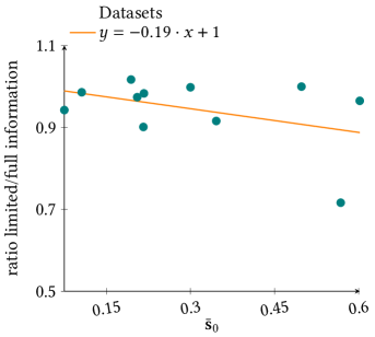
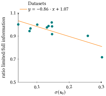
(a) initial disagreement, $R^{2}=0.08$	(b) average innate opinion, $R^{2}=0.17$	(c) standard deviation of opinions, $R^{2}=0.62$

Figure 2: Regression analysis of dataset parameters and the ratio between the best methods with full and limited information.

Dependency on $k$. For $k=0.5\%\,n,1\%\,n,\dots,2.5\%\,n$, we present our results on Tweet:L2 and Gplus:L2 in Figure 3. The figure indicates that the disagreement grows linearly in $k$; this behavior was also suggested by the upper bounds of Chen and Racz [13] and Gaitonde et al. [21] who considered a slightly stronger adversary. Similar to the results in Table 2, AG-F is the best method, followed by NAG-L and AG-L. The ranking of the algorithms is consistent across the different values of $k$. This answers RQ4.

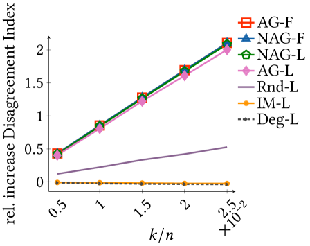
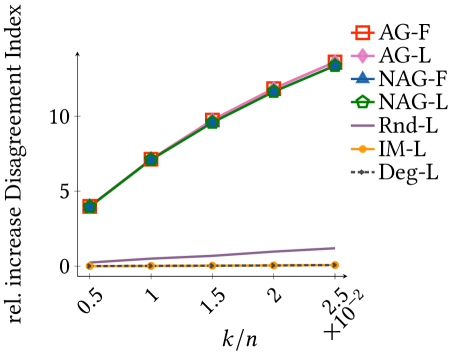
(a) Tweet:L2	(b) Gplus:L2

Figure 3: Results for the relative increase of the disagreement on Tweet:L2 and Gplus:L2. Here, we vary $k=0.5\%\,n,1\%\,n,\dots,2.5\%\,n$.

Additional experiments. In the appendix we present additional experiments. First, in Appendix A.3 we evaluate the algorithms for solving Problem (3.2). Second, in Appendix A.2 we also use our algorithms to maximize the polarization in the network; we remark that all of our results extend to this setting, including the guarantees from Theorem 3.3.

5 Conclusion

We have studied how adversaries can sow discord in social networks, even when they only have access to the network topology and cannot assess the opinions of the users. We proposed a framework in which we first detect a small set of users who are highly influential on the discord and then we change the opinions of these users. We showed experimentally that our approach can increase the discord significantly in practice and that it performs within a constant factor to the greedy algorithms that have access to the full information about the user opinions.

Our practical results demonstrate that attackers of social networks are quite powerful, even when they can only access the network topology. From an ethical point of view, these findings showcase the power of malicious attackers to sow discord and increase polarization in social networks. However, to draw a final conclusion further study is needed, for example because the assumption that the adversary can radicalize $k$ opinions arbitrarily much may be too strong. Nonetheless, the upshot is that by understanding attackers with limited information, one may be able to make recommendations to policy makers regarding the data that social-network providers can share with the public.

Furthermore, in this paper we only studied one possible definition for disagreement that is common in the computer science literature [13, 21]. Klofstad et al. [31] point out that in the political science literature there are different viewpoints on how disagreement should be defined, and that these different definitions will lead to different conclusions, with different empirical and democratic consequences. Understanding the connection of our definition and the ones in political science is an interesting question. Also, Edenberg [17] argues that to solve current societal problems like polarization, purely technical solutions, such as social media literacy campaigns and fact checking, are not enough; instead “we must find ways to cultivate mutual respect for our fellow citizens in order to reestablish common moral ground for political debate.” While certainly true, such considerations and course of actions are out of the scope of our paper.

As we already mentioned above, in future work it will be interesting to validate which adversary models are realistic in practice. Theoretically, it is interesting to obtain approximation algorithms for Problem (3.1) and the problem by Chen and Racz [13]; note that such algorithms must generalize our result from Theorem 3.3, as Problem (3.2) is a special case of Problem (3.1).

Appendix A Omitted Experiments

We present further details of our experiments. In Section A.1, we present details about our datasets. In Section A.2, we present how our algorithms perform when the goal is to maximize the polarization. In Section A.3 we compare different algorithms for finding users that are influential on the disagreement in the network (Problem (3.2)). In Section A.4 we discuss the stability of SDP-L and Rnd-L, which use randomization. In Section A.5 we present the running time of our algorithms.

Our algorithms are implemented in Python, except IMM [40] (related to our IM-L algorithm) which is implemented in Julia. We use Mosek to solve semidefinite programs.

A.1 Datasets

The datasets Tweet:S2, Tweet:S4, Tweet:M5, Tweet:L2 are sampled from a Twitter dataset with innate opinions, which we obtained from Tianyi Zhou. The original Twitter dataset is collected in the following way. We start from a list of Twitter accounts who actively engage in political discussions in the US, which was compiled by Garimella and Weber [24]. Then we randomly sample a smaller subset of 50 000 accounts. For these active accounts, we obtained the entire list of followers, except for users with more than 100 000 followers for whom we got only the 100 000 most recent followers (users with more than 100 000 followers account for less than 2% of our dataset). Based on this obtained information, we construct a graph in which the nodes correspond to Twitter accounts and the edges correspond to the accounts’ following relationships. Then we consider only the largest connected component in the network. To obtain the innate opinions of the nodes in the graphs, we proceed as follows. First, we compute the political polarity score for each account using the method proposed by Barberá [8], which has been used widely in the literature [11, 10]. The polarity scores range from -2 to 2 and are computed based on following known political accounts. Then we re-scale them into the interval $[0,1]$. To create our smaller datasets, we select a seed node uniformly at random, and run breadth-first search (BFS) from this seed node, until a given number of nodes have been explored.

We note that for Tweet:M5 and Tweet:L2, the innate opinions were very large ($\bar{\mathbf{s}}_{0}\geq 0.85$) and thus for these datasets we flipped the innate opinions around 0.5 (i.e., we set $\mathbf{s}_{0}=\mathbf{1}-\mathbf{s}_{0}$). In other words, we assume that initially most people are not on the extreme side of the opinion spectrum. By flipping the innate opinions, we guarantee that the attacker can still radicalize the opinions. We note that this has no influence on the the initial indices for polarization and disagreement (since for $\mathbf{A}\in\{{\mathcal{D}}(\mathbf{L})\,,{\mathcal{P}}(\mathbf{L})\,\}$ it holds that $\mathbf{s}_{0}^{\intercal}\mathbf{A}\mathbf{s}_{0}=(\mathbf{1}-\mathbf{s}_{0})^{\intercal}\mathbf{A}(\mathbf{1}-\mathbf{s}_{0})$ which is implied by Lemma 2.1).

The dataset Gplus:L2 is sampled from the ego-Gplus dataset obtained from SNAP [33] using the same BFS-approach as above. The innate opinions for Gplus:L2 are drawn independently from $N(0.3,0.1)$. Here, $N(\mu,\sigma)$ denotes the Gaussian distribution with mean $\mu$ and standard deviation $\sigma$.

We also use the publicfootnote 6 datasets Twitter and Reddit from De et al. [14], which have previously been used by Musco et al. [36] and Chen and Racz [13]. The Twitter dataset was obtained from tweets about the Delhi legislative assembly elections of 2013 and contains ground-truth opinions. The opinions for the Reddit dataset were generated by Musco et al. [36] using a power law distribution.

Furthermore, we consider the datasets karate, books, blogs, which we obtained from KONECT [32] and which do not contain ground-truth opinions. However, these datasets contain two ground-truth communities. For the first community, we sample the innate opinions of the users from the Gaussian distribution $N(0.1,0.1)$, and for the second community we use $N(0.3,0.1)$.

Last, we consider graphs generated from the Stochastic Block Model. We generate a Stochastic Block Model graph that consists of $1000$ nodes divided equally into $4$ communities. The intra-community edge probability is $0.4$ and an the inter-community edge probability is $0.1$. The innate opinions for each community are drawn from $N(0.2,0.1)$, $N(0.3,0.1)$, $N(0.4,0.1)$ and $N(0.5,0.1)$, respectively.

A.2 Maximizing the polarization

Next, we use our algorithms to maximize the polarization. We remark that all of our results extend to this setting, including the guarantees from Theorem 3.3.

We report our results on larger datasets with $k=1\%n$ in Table 3. For each of the datasets, we provide the number of vertices and edges. We also report the normalized polarization index $\mathcal{P}_{G,\mathbf{s}}^{\prime}=\frac{\mathcal{P}_{G,\mathbf{s}}\cdot 10^{5}}{\left\lvert V\right\rvert}$, where we normalize by the number of vertices for better comparison across different datasets. Further, we report average innate opinions $\bar{\mathbf{s}}_{0}$ and the standard deviation of the innate opinions $\sigma(\mathbf{s}_{0})$. Finally, as before, for each algorithm we report the score $\frac{\mathbf{s}^{\intercal}{\mathcal{P}}(\mathbf{L})\,\mathbf{s}-\mathbf{s}_{0}^{\intercal}{\mathcal{P}}(\mathbf{L})\,\mathbf{s}_{0}}{\mathbf{s}_{0}^{\intercal}{\mathcal{P}}(\mathbf{L})\,\mathbf{s}_{0}}$.

Table 3: Results on the larger datasets for the relative increase of the polarization, where we set $k=1\%n$. For each dataset, we have marked the highest value in bold and we have made the highest value for each setting italic.

dataset	$\left\lvert V\right\rvert$	$\left\lvert E\right\rvert$	$\mathcal{P}_{G,{\mathbf{s}_{0}}}^{\prime}$	$\bar{\mathbf{s}}_{0}$	$\sigma(\mathbf{s}_{0})$	full information		limited information
						NAG-F	AG-F	NAG-L	AG-L	Deg-L	IM-L	Rnd-L
Tweet:S2	$1\,999$	$40\,498$	$182.879$	$0.216$	$0.258$	$0.790$	0.792	0.692	0.692	$-0.016$	$-0.014$	$0.053$
Tweet:S4	$3\,999$	$222\,268$	$176.525$	$0.568$	$0.302$	0.273	0.273	0.188	$0.186$	$-0.008$	$-0.006$	$0.003$
Tweet:M5	$4\,999$	$245\,085$	$35.005$	$0.075$	$0.077$	$5.875$	5.876	5.258	5.258	$-0.035$	$-0.035$	$0.160$
Tweet:L2	$21\,999$	$860\,884$	$117.790$	$0.106$	$0.136$	$1.859$	1.865	1.579	$1.481$	$-0.029$	$-0.022$	$0.140$
Gplus:L2	$22\,999$	$5\,474\,133$	$1.803$	$0.300$	$0.101$	$30.351$	30.804	$30.338$	30.786	$0.002$	$0.001$	$0.441$

We see that the results for polarization are somewhat similar to those for disagreement: algorithms with full information are the best, but the best algorithm that only knows the topology still achieves similar performance.

Furthermore, the best algorithms with limited information, i.e., AG-L and NAG-L, consistently outperform the baselines Deg-L, IM-L, and Rnd-L; this shows that our strategy leads to non-trivial results. Furthermore, we observe that across all settings, simply picking high-degree vertices, or picking nodes with large influence in the independent cascade model are poor strategies.

In addition, we show results for the increase of polarization in the small datasets in Table 4. Again, the methods with full information perform best, and again our methods generally perform quite well and clearly outperform the baseline methods.

Table 4: Results on the small datasets for the relative increase of the polarization, where we set $k=10\%\,n$. For each dataset, we have marked the highest value in bold and we have made the highest value for each setting italic.

dataset	$\left\lvert V\right\rvert$	$\left\lvert E\right\rvert$	$\mathcal{P}_{G,{\mathbf{s}_{0}}}^{\prime}$	$\bar{\mathbf{s}}_{0}$	$\sigma(\mathbf{s}_{0})$	full information		limited information
						NAG-F	AG-F	SDP-L	NAG-L	AG-L	Deg-L	IM-L	Rnd-L
karate	$34$	$78$	$479.556$	$0.194$	$0.146$	$2.407$	2.412	1.702	$1.137$	$1.346$	$0.391$	$0.064$	$0.870$
books	$105$	$441$	$519.208$	$0.217$	$0.147$	$2.955$	3.009	2.149	$0.282$	2.149	$-0.229$	$-0.179$	$0.267$
Twitter	$548$	$3\,638$	$30.372$	$0.602$	$0.080$	$6.996$	8.941	$8.505$	$6.695$	8.526	$1.899$	$0.248$	$1.563$
Reddit	$556$	$8\,969$	$0.952$	$0.498$	$0.042$	$132.834$	133.258	133.225	$132.759$	133.225	$1.741$	$2.529$	$14.524$
SBM	$1000$	$74568$	$0.166$	$0.346$	$0.147$	$2.000$	2.146	2.014	$1.182$	$1.867$	$0.676$	$0.660$	$0.954$
blogs	$1\,222$	$16\,717$	$544.049$	$0.205$	$0.131$	$12.686$	12.789	$12.576$	12.614	$12.217$	$0.211$	$0.205$	$2.686$

A.3 Finding influential users

In this section, we evaluate different methods for finding the influential users which can maximize the disagreement. More specifically, we evaluate different methods for solving Problem (3.2).

We report our results in Figure 4. Notice that when $\mathbf{s}=\mathbf{1}$ and $k=0$, the disagreement is 0. Thus, instead of evaluating the relative gain of the Disagreement Index, we report absolute values of the Disagreement Index.

We observe that the baselines which pick random seed nodes, high degree nodes, and nodes with high influence in the independent cascade model are clearly the worst methods. Among the other methods, the SDP-based methods are typically the best. We observe that when $k$ is below $0.25n$, the greedy methods AG and NAG often perform as well as SDP; however, when $k$ is larger than $0.3n$, the SDP-based algorithm performs better. These observations are in line with the analysis of Theorem 3.3 which achieves the best approximation ratios when $k$ is close to $0.5n$ (see also Figure 1).

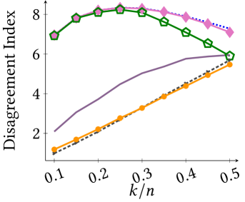
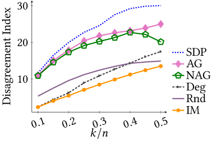
(a) Reddit	(b) Twitter
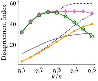
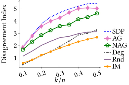
(c) blogs	(d) books

Figure 4: Results for Problem (3.2) on different datasets. We varied $k=10\%n,15\%n,...,50\%n$.

A.4 Stability of randomized algorithms

In this section, we study how the randomization involved in some of the algorithms affects their results. In particular, Rnd-L and SDP-L randomly select nodes and we wish to study how this impacts their performance. We report the Disagreement Index and output the mean over 5 runs of the algorithms, together with error bars that indicate standard deviations.

In Figure 5 we present the Disagreement Index and the standard deviation with randomized algorithms on small datasets. We observe that as the number of nodes increases, the standard deviations of different algorithms becomes relatively small (note that the largest dataset below is blogs). Besides, we also observe that the outputs of SDP-L are stable, with standard deviations close to 0.

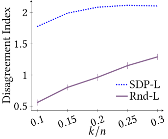
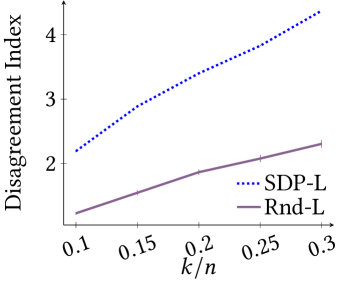
(a) Reddit	(b) Twitter
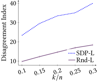
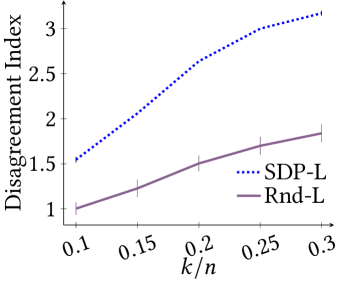
(c) blogs	(d) books

Figure 5: Results of our randomized algorithms for Problem (3.2) on different datasets. We varied $k=10\%n,15\%n,...,30\%n$ and report averages and standard deviations over 5 runs of the algorithms.

In Figure 6 we present results on larger graphs, Tweet:L2 and Gplus:L2; here, we omit SDP-L due to scalability issues.

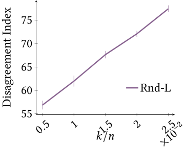
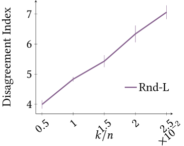
(a) Tweet:L2	(b) Gplus:L2

Figure 6: Results of Rnd-L for Problem (3.2) on different datasets. We varied $k=0.5\%n,1\%n,...,2.5\%n$ and report averages and standard deviations over 5 runs of the algorithms.

A.5 Running time of algorithms

Next, we present the running time of the algorithms to maximize the disagreement on different datasets. Note that for full information algorithms we directly present the running time, while for limited information algorithms we report the running time for solving Problem (3.2). This is because the running time for setting the innate opinions to $1$ is negligible. In addition, since the running times of AG-F and AG-L are almost the same, we only report the running time of AG-F. The same holds for NAG-F and NAG-L.

In Figure 7, we notice that AG-F and IM-L are the two most costly algorithms, but even for those algorithm the running time increases moderately in terms of $k$. However, on the less dense graph Tweet:L2, IM-L runs faster than on the denser graph Gplus:L2, even though they have almost the same number of vertices. This is consistent with the time complexity of IMM [40]. The graph density does not influence the running time of the adaptive greedy algorithm AG-F. Interestingly, we observe that that NAG-F is orders of magnitude faster than AG-F.

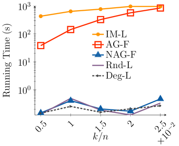
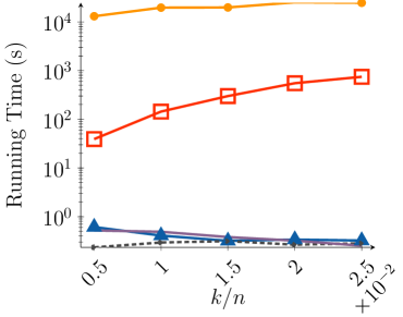
(a) Tweet:L2	(b) Gplus:L2

Figure 7: Running time (in seconds) of our algorithms for increasing the disagreement on Tweet:L2 and Gplus:L2. Here, we vary $k=0.5\%n$, $1\%n$, $1.5\%n$, $2\%n$, $2.5\%n$.

In Table 5 we report the absolute running times (in seconds) of our algorithms on the small datasets. We notice that SDP-L is the slowest algorithm and on blogs it is almost 30 times slower than any other algorithm. This is within our expectation, since solving semidefinite programs is costly. We again observe that that NAG-F is orders of magnitude faster than AG-F.

Table 5: Running time (in seconds) of our algorithms for maximizing the disagreement, where we set $k=10\%n$.

dataset	AG-F	NAG-F	SDP-L	IM-L	Deg-L	Rnd-L
karate	$0.0002$	$0.0000$	$0.0818$	$0.4506$	$0.0005$	$0.0001$
books	$0.0022$	$0.0001$	$0.4083$	$0.5041$	$0.0006$	$0.0001$
Twitter	$0.1832$	$0.0008$	$10.2997$	$1.3165$	$0.0018$	$0.0002$
Reddit	$0.1914$	$0.0009$	$9.6022$	$2.8257$	$0.0019$	$0.0002$
SBM	$1.2505$	$0.0030$	$72.8223$	$30.1188$	$0.0036$	$0.0006$
blogs	$3.9573$	$0.0052$	$171.4392$	$5.8961$	$0.0055$	$0.0007$

Appendix B Omitted Proofs and Discussions

We present proofs and discussions which are not contained in the main content below.

B.1 Rescaling Opinions

In Section 2, we mention that we consider the opinions in the interval $[0,1]$. In this appendix we prove that scaling the opinions from an interval $[a,b]$ to an interval $[x,y]$ only influences the disagreement in the network by a fixed factor of $\left(\frac{y-x}{b-a}\right)^{2}$. In particular, we show that the optimizers of optimization problems are maintained under scaling. This implies that all $\mathbf{NP}$-hardness results we derive in this paper carry over to the setting with $[-1,1]$-opinions and our $O(1)$-approximation algorithms for $[-1,1]$-opinions also yield $O(1)$-approximation algorithms for $[0,1]$-opinions.

Consider real numbers $a<b$ and $x<y$. Suppose that we have innate opinions $\mathbf{s}_{u}\in[a,b]$ and we wish to rescale them into the interval $[x,y]$. Then we set

$$\mathbf{s}_{u}^{\prime}=\mathbf{s}_{u}\cdot\frac{y-x}{b-a}+\frac{1}{2}\left(x+y-\frac{a+b}{b-a}(y-x)\right).$$

For convenience we set $\alpha=\frac{y-x}{b-a}$ and $\beta=\frac{1}{2}\left(x+y-\frac{a+b}{b-a}(y-x)\right)$. Observe that $\mathbf{s}_{u}^{\prime}=\alpha\mathbf{s}_{u}+\beta$. We also set $\mathbf{z}_{u}^{\prime(0)}=\alpha\mathbf{z}_{u}^{\prime(0)}+\beta$.

Indeed, let $f(\xi)=\alpha\xi+\beta$. Then we note that under this transformation we have that

$$f(a) =a\frac{y-x}{b-a}+\frac{1}{2}\left(x+y-\frac{a+b}{b-a}(y-x)\right)$$

$$=\frac{1}{2}\left(2a\frac{y-x}{b-a}+x+y-\frac{a+b}{b-a}(y-x)\right)$$

$$=\frac{1}{2}\left(x+y-\frac{b-a}{b-a}(y-x)\right)$$

$$=x,$$

and

$$f(b) =b\frac{y-x}{b-a}+\frac{1}{2}\left(x+y-\frac{a+b}{b-a}(y-x)\right)$$

$$=\frac{1}{2}\left(2b\frac{y-x}{b-a}+x+y-\frac{a+b}{b-a}(y-x)\right)$$

$$=\frac{1}{2}\left(x+y-\frac{a-b}{b-a}(y-x)\right)$$

$$=y.$$

Additionally, note that $f(\xi)$ is an affine linear function. Hence, $f$ maps $[a,b]$ bijectively into $[x,y]$.

Next, consider the expressed opinion $\mathbf{z}_{u}^{\prime(t+1)}$ then by the update rule of the FJ model and by induction we have that

$$\mathbf{z}_{u}^{\prime(t+1)} =\frac{\mathbf{s}_{u}^{\prime}+\sum_{v\in N(u)}w_{uv}\mathbf{z}_{u}^{\prime(t)}}{1+\sum_{v\in N(u)}w_{uv}}$$

$$=\frac{\alpha\mathbf{s}_{u}+\beta+\sum_{v\in N(u)}w_{uv}(\alpha\mathbf{z}_{u}^{(t)}+\beta)}{1+\sum_{v\in N(u)}w_{uv}}$$

$$=\alpha\frac{\mathbf{s}_{u}^{\prime}+\sum_{v\in N(u)}w_{uv}\mathbf{z}_{u}^{\prime(t)}}{1+\sum_{v\in N(u)}w_{uv}}+\beta$$

$$=\alpha\mathbf{z}_{u}^{(t+1)}+\beta.$$

In particular, in the limit we have that $\mathbf{z}^{\prime}=\lim_{t\to\infty}\mathbf{z}^{\prime(t+1)}=\lim_{t\to\infty}(\alpha\mathbf{z}^{(t+1)}+\beta)=\alpha\mathbf{z}+\beta$.

Next, for the disagreement in the network we have that:

$$\mathcal{D}_{G,\mathbf{s}^{\prime}} =\sum_{(u,v)\in E}w_{u,v}(\mathbf{z}_{u}^{\prime}-\mathbf{z}_{v}^{\prime})^{2}$$

$$=\sum_{(u,v)\in E}w_{u,v}(\alpha\mathbf{z}_{u}+\beta-\alpha\mathbf{z}_{v}-\beta)^{2}$$

$$=\alpha^{2}\sum_{(u,v)\in E}w_{u,v}(\mathbf{z}_{u}-\mathbf{z}_{v})^{2}$$

$$=\alpha^{2}\mathcal{D}_{G,\mathbf{s}^{\prime}}.$$

Now we consider the mean opinion $\bar{\mathbf{z}}^{\prime}$:

$$\bar{\mathbf{z}}^{\prime} =\frac{1}{n}\sum_{u}\mathbf{z}_{u}^{\prime}$$

$$=\frac{1}{n}\sum_{u}(\alpha\mathbf{z}_{u}+\beta)$$

$$=\alpha\left(\frac{1}{n}\sum_{u}\mathbf{z}_{u}\right)+\beta$$

$$=\alpha\bar{\mathbf{z}}+\beta.$$

Hence, for the network polarization we obtain:

$$\mathcal{P}_{G,\mathbf{s}^{\prime}} =\sum_{u\in V}(\mathbf{z}_{u}^{\prime}-\bar{\mathbf{z}}^{\prime})^{2}$$

$$=\sum_{u\in V}(\alpha\mathbf{z}_{u}+\beta-\alpha\bar{\mathbf{z}}-\beta)^{2}$$

$$=\alpha^{2}\sum_{u\in V}(\mathbf{z}_{u}-\bar{\mathbf{z}})^{2}$$

$$=\alpha^{2}\mathcal{P}_{G,\mathbf{s}^{\prime}}.$$

We note that the results from above hold for all vectors $\mathbf{s}\in[a,b]^{n}$. In particular, this implies that if $\mathbf{s}^{*}$ is the optimizer for an optimization problem of the form $\max_{\mathbf{s}\in[a,b]^{n}}\mathcal{D}_{G,\mathbf{s}^{\prime}}$ then the vector $f(\mathbf{s})\in[x,y]^{n}$ is the maximizer for the optimization problem $\max_{\mathbf{s}\in[x,y]^{n}}\mathcal{D}_{G,\mathbf{s}^{\prime}}$.

B.2 Proof of Lemma 2.1

We start by recalling two facts about positive semi-definite matrices. First, a matrix $\mathbf{A}$ is positive semi-definite if $\mathbf{A}=\mathbf{B}^{\intercal}\mathbf{C}\mathbf{B}$, where $\mathbf{C}$ is a positive semi-definite matrix. Second, $\mathbf{A}$ is positive semi-definite if we can write it as $\mathbf{A}=\mathbf{B}^{\intercal}\mathbf{B}$.

Let us consider the matrix ${\mathcal{P}}(\mathbf{L})\,=(\mathbf{I}+\mathbf{L})^{-1}\left(\mathbf{I}-\frac{\mathbf{1}\mathbf{1}^{\intercal}}{n}\right)(\mathbf{I}+\mathbf{L})^{-1}$ for polarization. Observe that $\mathbf{I}-\frac{\mathbf{1}\mathbf{1}^{\intercal}}{n}$ is the Laplacian of the full graph with edge weights $1/n$ and, hence, this matrix positive semi-definite. By our first property from above and the fact that $(\mathbf{I}+\mathbf{L})^{-1}$ is symmetric, this implies that ${\mathcal{P}}(\mathbf{L})\,$ is positive semidefinite. Proving that ${\mathcal{D}}(\mathbf{L})\,=(\mathbf{L}+\mathbf{I})^{-1}\mathbf{L}(\mathbf{L}+\mathbf{I})^{-1}$ is positive semi-definite works in the same way.

Next, we observe that $(\mathbf{I}+\mathbf{L})^{-1}$ satisfies $(\mathbf{I}+\mathbf{L})^{-1}\mathbf{1}=\mathbf{1}$ since $(\mathbf{I}+\mathbf{L})\mathbf{1}=\mathbf{1}+\mathbf{L}\mathbf{1}=\mathbf{1}$ and by multiplying with $(\mathbf{I}+\mathbf{L})^{-1}$ from both sides we obtain the claim.

Now we apply the previous observation for our matrices from the table and obtain

$${\mathcal{P}}(\mathbf{L})\,\mathbf{1}=(\mathbf{I}+\mathbf{L})^{-1}\left(\mathbf{I}-\frac{\mathbf{1}\mathbf{1}^{\intercal}}{n}\right)(\mathbf{I}+\mathbf{L})^{-1}\mathbf{1}=(\mathbf{I}+\mathbf{L})^{-1}\left(\mathbf{I}-\frac{\mathbf{1}\mathbf{1}^{\intercal}}{n}\right)\mathbf{1}=\mathbf{0}.$$

And,

$${\mathcal{D}}(\mathbf{L})\,\mathbf{1}=(\mathbf{L}+\mathbf{I})^{-1}\mathbf{L}(\mathbf{L}+\mathbf{I})^{-1}\mathbf{1}=(\mathbf{L}+\mathbf{I})^{-1}\mathbf{L}\mathbf{1}=\mathbf{0}.$$

B.3 Proof of Theorem 3.2

Consider the optimal solution $\mathbf{s}_{\mathbf{OPT}}$ for Problem 3.1 and let $\mathbf{s}_{\mathbf{ALG}}$ denote the $\beta$-approximate solution for Problem 3.2. Furthermore, set $\mathbf{\Delta}_{\mathbf{OPT}}=\mathbf{s}_{\mathbf{OPT}}-\mathbf{s}_{0}$ and $\mathbf{\Delta}_{\mathbf{ALG}}=\mathbf{s}_{\mathbf{ALG}}-\mathbf{s}_{0}$.

Then we get that

$$\frac{\mathbf{s}_{\mathbf{ALG}}^{\intercal}\mathbf{A}\mathbf{s}_{\mathbf{ALG}}}{\mathbf{s}_{\mathbf{OPT}}^{\intercal}\mathbf{A}\mathbf{s}_{\mathbf{OPT}}}$$

$$=\frac{(c\mathbf{1}+\hat{\mathbf{r}}+\mathbf{\Delta}_{\mathbf{ALG}})^{\intercal}\mathbf{A}(c\mathbf{1}+\hat{\mathbf{r}}+\mathbf{\Delta}_{\mathbf{ALG}})}{(c\mathbf{1}+\hat{\mathbf{r}}+\mathbf{\Delta}_{\mathbf{OPT}})^{\intercal}\mathbf{A}(c\mathbf{1}+\hat{\mathbf{r}}+\mathbf{\Delta}_{\mathbf{OPT}})}$$

$$=\frac{(\hat{\mathbf{r}}+\mathbf{\Delta}_{\mathbf{ALG}})^{\intercal}\mathbf{A}(\hat{\mathbf{r}}+\mathbf{\Delta}_{\mathbf{ALG}})}{(\hat{\mathbf{r}}+\mathbf{\Delta}_{\mathbf{OPT}})^{\intercal}\mathbf{A}(\hat{\mathbf{r}}+\mathbf{\Delta}_{\mathbf{OPT}})}$$

$$=\frac{\mathbf{\Delta}_{\mathbf{ALG}}^{\intercal}\mathbf{A}\mathbf{\Delta}_{\mathbf{ALG}}+2\hat{\mathbf{r}}^{\intercal}\mathbf{A}\mathbf{\Delta}_{\mathbf{ALG}}+\hat{\mathbf{r}}^{\intercal}\mathbf{A}\hat{\mathbf{r}}}{\mathbf{\Delta}_{\mathbf{OPT}}^{\intercal}\mathbf{A}\mathbf{\Delta}_{\mathbf{OPT}}+2\hat{\mathbf{r}}^{\intercal}\mathbf{A}\mathbf{\Delta}_{\mathbf{OPT}}+\hat{\mathbf{r}}^{\intercal}\mathbf{A}\hat{\mathbf{r}}}$$

$$\geq\frac{\mathbf{\Delta}_{\mathbf{ALG}}^{\intercal}\mathbf{A}\mathbf{\Delta}_{\mathbf{ALG}}+(1-2\gamma_{1})\hat{\mathbf{r}}^{\intercal}\mathbf{A}\hat{\mathbf{r}}}{\mathbf{\Delta}_{\mathbf{OPT}}^{\intercal}\mathbf{A}\mathbf{\Delta}_{\mathbf{OPT}}+2\hat{\mathbf{r}}^{\intercal}\mathbf{A}\mathbf{\Delta}_{\mathbf{OPT}}+\hat{\mathbf{r}}^{\intercal}\mathbf{A}\hat{\mathbf{r}}}$$

$$\geq\frac{\mathbf{\Delta}_{\mathbf{ALG}}^{\intercal}\mathbf{A}\mathbf{\Delta}_{\mathbf{ALG}}+(1-2\gamma_{1})\hat{\mathbf{r}}^{\intercal}\mathbf{A}\hat{\mathbf{r}}}{2(\mathbf{\Delta}_{\mathbf{OPT}}^{\intercal}\mathbf{A}\mathbf{\Delta}_{\mathbf{OPT}}+\hat{\mathbf{r}}^{\intercal}\mathbf{A}\hat{\mathbf{r}})},$$

where in the first step we used the assumption $\mathbf{s}_{0}=c\mathbf{1}+\hat{\mathbf{r}}$ and the definitions of $\mathbf{\Delta}_{\mathbf{ALG}}$ and $\mathbf{\Delta}_{\mathbf{OPT}}$. In the second step we used that $\mathbf{A}\mathbf{1}=\mathbf{0}$ by Lemma 2.1 and that $\mathbf{A}$ is symmetric. In the fourth step we used Assumption (1) and the observations that $\mathbf{s}_{\mathbf{ALG}}-\mathbf{s}_{0}=\mathbf{\Delta}_{\mathbf{ALG}}$ and $\mathbf{s}_{0}^{\intercal}\mathbf{A}=(c\mathbf{1}+\hat{\mathbf{r}})^{\intercal}\mathbf{A}=\hat{\mathbf{r}}^{\intercal}\mathbf{A}$ using Lemma 2.1. In the fifth step we used that $2\hat{\mathbf{r}}^{\intercal}\mathbf{A}\mathbf{\Delta}_{\mathbf{OPT}}\leq\mathbf{\Delta}_{\mathbf{OPT}}^{\intercal}\mathbf{A}\mathbf{\Delta}_{\mathbf{OPT}}+\hat{\mathbf{r}}^{\intercal}\mathbf{A}\hat{\mathbf{r}}$. The last fact can be seen by letting $\mathbf{A}=D^{\intercal}D$ for a suitable matrix $D$ (which exists since $\mathbf{A}$ is positive semi-definite by Lemma 2.1) and observing that $0\leq||D(\mathbf{\Delta}_{\mathbf{OPT}}-\hat{\mathbf{r}})||_{2}^{2}=(\mathbf{\Delta}_{\mathbf{OPT}}-\hat{\mathbf{r}})^{\intercal}D^{\intercal}D(\mathbf{\Delta}_{\mathbf{OPT}}-\hat{\mathbf{r}})=\mathbf{\Delta}_{\mathbf{OPT}}^{\intercal}\mathbf{A}\mathbf{\Delta}_{\mathbf{OPT}}-2\hat{\mathbf{r}}^{\intercal}\mathbf{A}\mathbf{\Delta}_{\mathbf{OPT}}+\hat{\mathbf{r}}^{\intercal}\mathbf{A}\hat{\mathbf{r}}$; by rearranging terms we obtain the claimed inequality.

Next, we let $\mathbf{OPT}\subseteq V$ denote the set of nodes such that $\mathbf{s}_{0}(u)\neq\mathbf{s}_{\mathbf{OPT}}(u)$ and similarly we set $\mathbf{ALG}\subseteq V$ to the set of nodes with $\mathbf{s}_{0}(u)\neq\mathbf{s}_{\mathbf{ALG}}(u)$. Observe that since $\mathbf{s}_{\mathbf{OPT}}=c\mathbf{1}+\hat{\mathbf{r}}+\mathbf{\Delta}_{\mathbf{OPT}}$ and $\mathbf{s}_{\mathbf{OPT}}(u)=1$ for all $u\in\mathbf{OPT}$, we have that $\mathbf{\Delta}_{\mathbf{OPT}}=(1-c)\mathbf{1}_{|\mathbf{OPT}}-\hat{\mathbf{r}}_{|\mathbf{OPT}}$. Similarly, $\mathbf{\Delta}_{\mathbf{ALG}}=(1-c)\mathbf{1}_{|\mathbf{ALG}}-\hat{\mathbf{r}}_{|\mathbf{ALG}}$.

Then we get that

$$\mathbf{\Delta}_{\mathbf{ALG}}^{\intercal}\mathbf{A}\mathbf{\Delta}_{\mathbf{ALG}}$$

$$=(1-c)^{2}\mathbf{1}_{|\mathbf{ALG}}^{\intercal}\mathbf{A}\mathbf{1}_{|\mathbf{ALG}}-2(1-c)\hat{\mathbf{r}}_{|\mathbf{ALG}}^{\intercal}\mathbf{A}\mathbf{1}_{|\mathbf{ALG}}$$

$$\quad+\hat{\mathbf{r}}_{|\mathbf{ALG}}^{\intercal}\mathbf{A}\hat{\mathbf{r}}_{|\mathbf{ALG}}$$

$$\geq(1-c)^{2}\mathbf{1}_{|\mathbf{ALG}}^{\intercal}\mathbf{A}\mathbf{1}_{|\mathbf{ALG}}-2(1-c)\hat{\mathbf{r}}_{|\mathbf{ALG}}^{\intercal}\mathbf{A}\mathbf{1}_{|\mathbf{ALG}}$$

$$\geq(1-c)^{2}\mathbf{1}_{|\mathbf{ALG}}^{\intercal}\mathbf{A}\mathbf{1}_{|\mathbf{ALG}}-2(1-c)\gamma_{3}\hat{\mathbf{r}}^{\intercal}\mathbf{A}\hat{\mathbf{r}},$$

where in the second step we used that $\hat{\mathbf{r}}_{|\mathbf{ALG}}\mathbf{A}\hat{\mathbf{r}}_{|\mathbf{ALG}}\geq 0$ and in the third step we used Assumption (3).

Furthermore, we obtain that

$$\mathbf{\Delta}_{\mathbf{OPT}}^{\intercal}\mathbf{A}\mathbf{\Delta}_{\mathbf{OPT}}$$

$$=(1-c)^{2}\mathbf{1}_{|\mathbf{OPT}}^{\intercal}\mathbf{A}\mathbf{1}_{|\mathbf{OPT}}-2(1-c)\hat{\mathbf{r}}_{|\mathbf{OPT}}^{\intercal}\mathbf{A}\mathbf{1}_{|\mathbf{OPT}}$$

$$\quad+\hat{\mathbf{r}}_{|\mathbf{OPT}}^{\intercal}\mathbf{A}\hat{\mathbf{r}}_{|\mathbf{OPT}}$$

$$\leq(1-c)^{2}\mathbf{1}_{|\mathbf{OPT}}^{\intercal}\mathbf{A}\mathbf{1}_{|\mathbf{OPT}}+(2(1-c)\gamma_{3}+\gamma_{2})\hat{\mathbf{r}}^{\intercal}\mathbf{A}\hat{\mathbf{r}},$$

where we used Assumptions (3) and (2).

By combining our derivations from above, we obtain that

$$\frac{\mathbf{s}_{\mathbf{ALG}}^{\intercal}\mathbf{A}\mathbf{s}_{\mathbf{ALG}}}{\mathbf{s}_{\mathbf{OPT}}^{\intercal}\mathbf{A}\mathbf{s}_{\mathbf{OPT}}}$$

$$\geq\frac{(1-c)^{2}\mathbf{1}_{|\mathbf{ALG}}^{\intercal}\mathbf{A}\mathbf{1}_{|\mathbf{ALG}}+(1-2\gamma_{1}-2(1-c)\gamma_{3})\hat{\mathbf{r}}^{\intercal}\mathbf{A}\hat{\mathbf{r}}}{2((1-c)^{2}\mathbf{1}_{|\mathbf{OPT}}^{\intercal}\mathbf{A}\mathbf{1}_{|\mathbf{OPT}}+(1+2(1-c)\gamma_{3}+\gamma_{2})\hat{\mathbf{r}}^{\intercal}\mathbf{A}\hat{\mathbf{r}})}.$$

Next, let $\mathbf{s}_{\mathbf{OPT}^{\prime}}\in\{0,1\}^{n}$ denote the optimal solution for Problem 3.2. Furthermore, observe that $\mathbf{1}_{|\mathbf{OPT}}$ and $\mathbf{1}_{|\mathbf{ALG}}$ are feasible solutions for Problem 3.2. Hence, we obtain

$$\mathbf{1}_{|\mathbf{OPT}}^{\intercal}\mathbf{A}\mathbf{1}_{|\mathbf{OPT}}\leq\mathbf{s}_{\mathbf{OPT}^{\prime}}^{\intercal}\mathbf{A}\mathbf{s}_{\mathbf{OPT}^{\prime}}.$$

Furthermore, since in our algorithm we use an $\beta$-approximation algorithm for Problem 3.2 to pick the set of nodes $\mathbf{ALG}$, it also holds that

$$\mathbf{1}_{|\mathbf{ALG}}^{\intercal}\mathbf{A}\mathbf{1}_{|\mathbf{ALG}}\geq\beta\cdot\mathbf{s}_{\mathbf{OPT}^{\prime}}^{\intercal}\mathbf{A}\mathbf{s}_{\mathbf{OPT}^{\prime}}.$$

This implies that

$$\frac{\mathbf{s}_{\mathbf{ALG}}^{\intercal}\mathbf{A}\mathbf{s}_{\mathbf{ALG}}}{\mathbf{s}_{\mathbf{OPT}}^{\intercal}\mathbf{A}\mathbf{s}_{\mathbf{OPT}}}$$

$$\geq\frac{(1-c)^{2}\beta\mathbf{s}_{\mathbf{OPT}^{\prime}}^{\intercal}\mathbf{A}\mathbf{s}_{\mathbf{OPT}^{\prime}}+(1-2\gamma_{1}-2(1-c)\gamma_{3})\hat{\mathbf{r}}^{\intercal}\mathbf{A}\hat{\mathbf{r}},}{2((1-c)^{2}\mathbf{s}_{\mathbf{OPT}^{\prime}}^{\intercal}\mathbf{A}\mathbf{s}_{\mathbf{OPT}^{\prime}}+(1+2(1-c)\gamma_{3}+\gamma_{2})\hat{\mathbf{r}}^{\intercal}\mathbf{A}\hat{\mathbf{r}})}.$$

To obtain our approximation, observe that if

$$(1-c)^{2}\mathbf{s}_{\mathbf{OPT}^{\prime}}^{\intercal}\mathbf{A}\mathbf{s}_{\mathbf{OPT}^{\prime}}\geq(1+2(1-c)\gamma_{3}+\gamma_{2})\hat{\mathbf{r}}^{\intercal}\mathbf{A}\hat{\mathbf{r}})$$

then

$$\frac{\mathbf{s}_{\mathbf{ALG}}^{\intercal}\mathbf{A}\mathbf{s}_{\mathbf{ALG}}}{\mathbf{s}_{\mathbf{OPT}}^{\intercal}\mathbf{A}\mathbf{s}_{\mathbf{OPT}}}$$

$$\geq\frac{(1-c)^{2}\beta\mathbf{s}_{\mathbf{OPT}^{\prime}}^{\intercal}\mathbf{A}\mathbf{s}_{\mathbf{OPT}^{\prime}}+(1-2\gamma_{1}-2(1-c)\gamma_{3})\hat{\mathbf{r}}^{\intercal}\mathbf{A}\hat{\mathbf{r}},}{4(1-c)^{2}\mathbf{s}_{\mathbf{OPT}^{\prime}}^{\intercal}\mathbf{A}\mathbf{s}_{\mathbf{OPT}^{\prime}}}$$

$$\geq\frac{\beta}{4}.$$

Similarly, if

$$(1-c)^{2}\mathbf{s}_{\mathbf{OPT}^{\prime}}^{\intercal}\mathbf{A}\mathbf{s}_{\mathbf{OPT}^{\prime}}<(1+2(1-c)\gamma_{3}+\gamma_{2})\hat{\mathbf{r}}^{\intercal}\mathbf{A}\hat{\mathbf{r}})$$

then

$$\frac{\mathbf{s}_{\mathbf{ALG}}^{\intercal}\mathbf{A}\mathbf{s}_{\mathbf{ALG}}}{\mathbf{s}_{\mathbf{OPT}}^{\intercal}\mathbf{A}\mathbf{s}_{\mathbf{OPT}}}$$

$$>\frac{(1-c)^{2}\beta\mathbf{s}_{\mathbf{OPT}^{\prime}}^{\intercal}\mathbf{A}\mathbf{s}_{\mathbf{OPT}^{\prime}}+(1-2\gamma_{1}-2(1-c)\gamma_{3})\hat{\mathbf{r}}^{\intercal}\mathbf{A}\hat{\mathbf{r}}}{4(1+2(1-c)\gamma_{3}+\gamma_{2})\hat{\mathbf{r}}^{\intercal}\mathbf{A}\hat{\mathbf{r}})}$$

$$\geq\frac{(1-2\gamma_{1}-2(1-c)\gamma_{3})}{4(1+2(1-c)\gamma_{3}+\gamma_{2})}.$$

We conclude that the approximation ratio of our algorithm is given by $\frac{1}{4}\min\{\beta,\frac{1-2\gamma_{1}-2(1-c)\gamma_{3}}{1+2(1-c)\gamma_{3}+\gamma_{2}}\}$.

B.4 Convexity Implies Extreme Values

Let $\mathbf{A}\in\mathbb{R}^{n\times n}$ be a symmetric matrix, let $\mathbf{s}_{0}\in[-1,1]^{n}$ and let $k>0$ be an integer. Consider the following optimization problem, which generalizes Problems (3.1), (3.2), and (3.3):

$$\max_{\mathbf{s}} \mathbf{s}^{\intercal}\mathbf{A}\mathbf{s},$$ (B.1)

such that $$\mathbf{s}\in[-1,1]^{n},\text{ and}$$

$$\lVert\mathbf{s}-\mathbf{s}_{0}\rVert_{0}\leq k.$$

Now we show prove a lemma about optimal solutions of Problem (B.1), where we write $\mathbf{x}(i)$ to denote the $i$’th entry of a vector $\mathbf{x}$.

Lemma B.1.

Suppose that $\mathbf{A}$ is a positive semi-definite matrix. Then there exists an optimal solution $\mathbf{s}$ for Problem B.1 such that $\mathbf{s}(i)\in\{-1,1\}$ for all entries $i$ with $\mathbf{s}(i)\neq\mathbf{s}_{0}(i)$. In particular, if $\mathbf{s}_{0}\in\{-1,1\}^{n}$ or $k=n$ then there exists an optimal solution $\mathbf{s}\in\{-1,1\}^{n}$.

Proof.

First, note that since $\mathbf{A}$ is positive semi-definite, the quadratic form $f(\mathbf{s})=\mathbf{s}^{\intercal}\mathbf{A}\mathbf{s}$ is convex.

Second, consider an optimal solution $\mathbf{s}$. If $\mathbf{s}$ satisfies the property from the lemma, we are done. Otherwise, there exists at least one entry $i$ such that $\mathbf{s}(i)\neq\mathbf{s}_{0}(i)$ and $\mathbf{s}(i)\in(0,1)$. Now let $\mathbf{t}_{-1}$ denote the vector which has its $i$’th entry set to $-1$ and in which all other entries are the same as in $\mathbf{s}$, i.e., $\mathbf{t}_{-1}(j)=\mathbf{s}(j)$ for all $j\neq i$ and $\mathbf{t}_{-1}(i)=-1$. Similarly, we set $\mathbf{t}_{1}$ to the vector with $\mathbf{t}_{1}(j)=\mathbf{s}(j)$ for all $j\neq i$ and $\mathbf{t}_{1}(i)=1$. Note that $\mathbf{t}_{-1}$ and $\mathbf{t}_{1}$ are feasible solutions to Problem (B.1).

Third, observe that there exists an $\alpha\in(0,1)$ such that $\mathbf{s}=\alpha\mathbf{t}_{-1}+(1-\alpha)\mathbf{t}_{1}$. Now by the convexity of $f(\mathbf{s})$ we get that

$$f(\mathbf{s}) =f(\alpha\mathbf{t}_{-1}+(1-\alpha)\mathbf{t}_{1})$$

$$\leq\alpha f(\mathbf{t}_{-1})+(1-\alpha)f(\mathbf{t}_{1})$$

$$\leq\max\{f(\mathbf{t}_{-1}),f(\mathbf{t}_{1})\}.$$

Thus, at least one of $\mathbf{t}_{-1}$ and $\mathbf{t}_{1}$ achieves an objective function value that is at least as large as that of $\mathbf{s}$. Hence, we can assume that the $i$’th entry of $\mathbf{s}$ is from the set $\{-1,1\}$. Repeating the above procedure for all entries with $\mathbf{s}(i)\neq\mathbf{s}_{0}(i)$ and $\mathbf{s}(i)\in(0,1)$ proves the first part of the lemma.

The second part of the lemma (if $\mathbf{s}_{0}\in\{-1,1\}^{n}$ or $k=n$) follows immediately from the first part. ∎

B.5 An illustration of graphs with mixed weights

Figure 8 shows how the cut of a graph can be influenced by positive and negative weights. We use this example to show that “badly-behaved” graphs with negative weights can make the cut value drop significantly, whereas in graphs with only positive edges this is not the case. The graphs we discuss in the paper are in the class of “well-behaved” graphs.

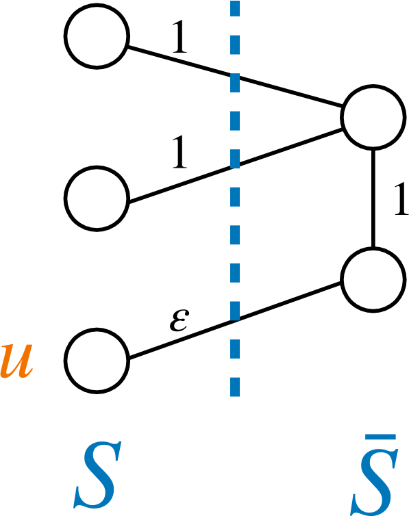
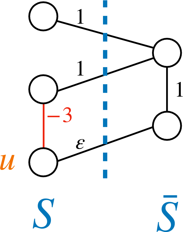
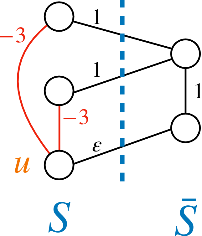
(a) Graph with	(b) “Well-behaved”	(c) “Badly-behaved”
positive weights	graph with	graph with
	negative weights	negative weights

Figure 8: We visualize cuts in a graph that partition the vertices into sets $S$ and $\bar{S}$; edge weights are also illustrated. The cut shown here has value $2+\epsilon$. Figure (a): A graph with positive edge weights. An averaging argument reveals that there must exist a vertex in $S$ that we can move to $\bar{S}$ such that the cut value is at least $\frac{2+\epsilon}{\left\lvert S\right\rvert}\geq\frac{2}{3}$. Indeed, if we move $u$ from $S$ to $\bar{S}$, the cut value drops only by $\epsilon$. Figure (b): In graphs with both positive and negative edge weights, the situation is less clear: if we move $u$ from $S$ to $\bar{S}$, the cut value becomes $-1$. However, in this example we could move the top-left vertex from $S$ to $\bar{S}$. Then we would still maintain a positive cut value, but it would drop to $1+\epsilon$. Note that this new cut value is strictly less than what the averaging argument from above revealed. Figure (c): In the worst case, it can happen that there exists no vertex in $S$, which we can move from $S$ to $\bar{S}$ without obtaining a negative cut value. In our proofs, we have to show that this scenario cannot occur in our setting. We prove this in Lemma 3.7.

B.6 Proof of Theorem 3.3

We start by defining notation. Let $\mathbf{OPT}$ denote the optimal solution for $\alpha$-Balanced-MaxCut, let $M_{0}$ be the objective function value obtained through randomized rounding after solving Problem (3.4), and let $M$ be the cut value for $(T,\bar{T})$ we obtain in the end. Let $M^{*}$ be the optimal solution for Problem (3.4).

We start with an overview of our analysis which is similar to the one by Frieze and Jerrum [20]. By solving the SDP and applying the hyperplane rounding enough times, we show that Lemma 3.6 implies that $M_{0}$ is close $(1-\epsilon)\frac{2}{\pi}\mathbf{OPT}$ and simultaneously $\left\lvert S_{0}\right\rvert\left\lvert\bar{S_{0}}\right\rvert=\left\lvert S_{0}\right\rvert(n-\left\lvert S_{0}\right\rvert)$ does not differ too much from $\alpha(1-\alpha)n^{2}$. This then implies that that the loss from the greedy procedure for ensuring the $\alpha$-balancedness constraint is not too large. To bound the loss from our greedy procedure for the size adjustments, we apply Lemma 3.8 with $(S_{0},\bar{S}_{0})$ corresponding to the (unbalanced) solution $(S,\bar{S})$ from the hyperplane rounding and $(T,\bar{T})$ corresponding to the $\alpha$-balanced solution that we return.

Next, we proceed with the concrete details of the proof. First, observe that since the objective function of the optimization problem is convex (see Section B.4) there exists an optimal solution with $\mathbf{s}\in\{-1,1\}^{n}$. Hence, we can focus on solutions with $\mathbf{s}\in\{-1,1\}^{n}$.

Consider the $p$-th iteration of Algorithm 1. Let $X_{p}$ denote the cut value of $(S,\bar{S})$, and let $Y_{p}=\left\lvert S\right\rvert\left\lvert\bar{S}\right\rvert$. Let $Z_{p}=\frac{X_{p}}{M^{*}}+\frac{Y_{p}}{N}$, where $N=\frac{n^{2}}{\beta}$ and $\beta\in(0,7]$ is a parameter that depends on $\alpha$ and that we will pick below. We use a similar approach as [20] to do the analysis.

By Lemma 3.6, $\mathbb{E}[Z_{p}]\geq\frac{2}{\pi}+0.878\alpha(1-\alpha)\cdot\beta$. As $X_{p}\leq M^{*}$ and $Y_{p}\leq\frac{n^{2}}{4}$, we obtain $Z_{p}\leq 1+\frac{\beta}{4}$. We will prove that in the $\kappa$ iterations of Algorithm 1, there exists a $\tau$ where $Z_{\tau}=\max_{p}Z_{p}$ such that $Z_{\tau}\geq(1-\epsilon)(\frac{2}{\pi}+0.878\alpha(1-\alpha)\cdot\beta)$ with probability at least $1-\epsilon$.

We first bound the probability of $Z_{p}\leq(1-\epsilon)\left(\frac{2}{\pi}+0.878\alpha(1-\alpha)\cdot\beta)\right)$ for a single iteration $p$ as follows:

$$\mathrm{Pr}\left(Z_{p}\leq(1-\epsilon)\left(\frac{2}{\pi}+0.878\alpha(1-\alpha)\cdot\beta)\right)\right)$$

$$=\mathrm{Pr}\left(\frac{\beta}{4}+1-Z_{p}\geq\frac{\beta}{4}+1-\left((1-\epsilon)\left(\frac{2}{\pi}+0.878\alpha(1-\alpha)\cdot\beta\right)\right)\right)$$

$$\leq\frac{\frac{\beta}{4}+1-\mathbb{E}[Z_{p}]}{\frac{\beta}{4}+1-((1-\epsilon)(\frac{2}{\pi}+0.878\alpha(1-\alpha)\cdot\beta))}$$

$$\leq\frac{\frac{\beta}{4}+1-(\frac{2}{\pi}+0.878\alpha(1-\alpha)\cdot\beta)}{\frac{\beta}{4}+1-((1-\epsilon)(\frac{2}{\pi}+0.878\alpha(1-\alpha)\cdot\beta))}$$

$$=\frac{1-c}{1-(1-\epsilon)c},$$

where $c=\frac{\frac{2}{\pi}+0.878\alpha(1-\alpha)\cdot\beta}{1+\frac{\beta}{4}}$. The first equality holds as we multiply with $-1$ and add $\frac{\beta}{4}+1$ to both sides; the first inequality holds by Markov inequality; the second inequality holds by $\mathbb{E}[Z_{p}]\geq 0.878\alpha(1-\alpha)\cdot\beta+\frac{2}{\pi}$. In the end we simplify the formula by introducing $c$. Notice that since we assume $\beta>0$, $c$ is in $(0,1)$. Moreover, by Lemma B.2, we can bound $c$ between $\frac{\frac{2}{\pi}}{1}$ and $\frac{0.878\alpha(1-\alpha)\cdot\beta}{\frac{\beta}{4}}$. Namely, either $c\in[{0.878\alpha(1-\alpha)\cdot 4},\frac{2}{\pi}]$ or $c\in[\frac{2}{\pi},{0.878\alpha(1-\alpha)\cdot 4}]$.

Lemma B.2.

Let $a_{1},a_{2},a_{3},a_{4}$ be positive real numbers, then either $\frac{a_{2}}{a_{4}}\leq\frac{a_{1}+a_{2}}{a_{3}+a_{4}}\leq\frac{a_{1}}{a_{3}}$ or $\frac{a_{2}}{a_{4}}\geq\frac{a_{1}+a_{2}}{a_{3}+a_{4}}\geq\frac{a_{1}}{a_{3}}$.

Proof.

We prove the lemma with two case distinctions.

Case 1: Assume $a_{1}a_{4}\geq a_{2}a_{3}$. If we add $a_{2}a_{4}$ on both sides, the formula becomes $(a_{1}+a_{2})a_{4}\geq a_{2}(a_{3}+a_{4})$, which implies $\frac{a_{1}+a_{2}}{a_{3}+a_{4}}\geq\frac{a_{2}}{a_{4}}$; if we add $a_{1}a_{3}$ on both sides, the formula becomes $a_{1}(a_{3}+a_{4})\geq(a_{1}+a_{2})a_{3}$, which implies $\frac{a_{1}}{a_{3}}\geq\frac{a_{1}+a_{2}}{a_{3}+a_{4}}$; thus $\frac{a_{1}}{a_{3}}\geq\frac{a_{1}+a_{2}}{a_{3}+a_{4}}\geq\frac{a_{2}}{a_{4}}$.

Case 2: Assume $a_{1}a_{4}\leq a_{2}a_{3}$. If we add $a_{2}a_{4}$ on both sides, the formula becomes $(a_{1}+a_{2})a_{4}\leq a_{2}(a_{3}+a_{4})$, which implies $\frac{a_{1}+a_{2}}{a_{3}+a_{4}}\leq\frac{a_{2}}{a_{4}}$; if we add $a_{1}a_{3}$ on both sides, the formula becomes $a_{1}(a_{3}+a_{4})\leq(a_{1}+a_{2})a_{3}$, which implies $\frac{a_{1}}{a_{3}}\leq\frac{a_{1}+a_{2}}{a_{3}+a_{4}}$; thus $\frac{a_{1}}{a_{3}}\leq\frac{a_{1}+a_{2}}{a_{3}+a_{4}}\leq\frac{a_{2}}{a_{4}}$. ∎

Notice that as the algorithm repeats the procedure $\kappa$ times, and the runs of the procedure are independent from each other, the probability that $Z_{p}\leq(1-\epsilon)(\frac{2}{\pi}+0.878\alpha(1-\alpha)\cdot\beta)$ for all $p$ is then bounded from above by

$$\left(\frac{1-c}{1-(1-\epsilon)c}\right)^{\kappa} =\left(1-\frac{1}{1+\frac{1-c}{\epsilon c}}\right)^{\kappa}$$

$$=\left(1-\frac{1}{1+\frac{1-c}{\epsilon c}}\right)^{(1+\frac{1-c}{\epsilon c})\frac{\epsilon c}{1-c+\epsilon c}\kappa}$$

$$\leq\exp\left(-\frac{\epsilon c}{1-c+\epsilon c}\kappa\right),$$

where the inequality holds through $(1-\frac{1}{x})^{x}\leq\frac{1}{e}$ for any $x>1$.

As a result, if we choose $\kappa\geq\frac{1-c+\epsilon c}{\epsilon c}\log(\frac{1}{\epsilon})\in\mathcal{O}(\frac{1}{\epsilon}\log(\frac{1}{\epsilon}))$, with probability at least $1-\epsilon$, $Z_{\tau}\geq(1-\epsilon)(\frac{2}{\pi}+0.878\alpha(1-\alpha)\cdot\beta)$.

Now consider the (non-$\alpha$-balanced) solution $(S,\bar{S})$ from the $\tau$-th iteration with cut-value $M_{0}:=X_{\tau}$. We set $s=\frac{\left\lvert S\right\rvert}{n}$ and $t=\alpha$ and apply Lemma 3.8 to obtain a solution that satisfies the $\alpha$-balancedness constraint. Suppose that in the $\tau$-th run, $X_{\tau}=\lambda M^{*}$ for suitable $\lambda$. Then it follows that $Y_{\tau}\geq((1-\epsilon)(0.878\alpha(1-\alpha)\cdot\beta+\frac{2}{\pi})-\lambda)N$. By replacing $Y_{\tau}$ with $Y_{\tau}=n^{2}(1-s)s$, we obtain $\lambda\geq(1-\epsilon)(\frac{\pi}{2}+0.878\alpha(1-\alpha)\cdot\beta)-\beta(1-s)s$.

We distinguish the two cases $0<s\leq t\leq 0.5$ and $0<t<s\leq 0.5$.

Case 1: $0<s<t\leq 0.5$. By Lemma 3.8 we have that $M\geq\frac{(1-t)^{2}-7(1-t)/n+12/n^{2}}{(1-s)^{2}+(1-s)/n}M_{0}$. Now notice that $\lim_{n\rightarrow\infty}\frac{(1-t)^{2}-7(1-t)/n+12/n^{2}}{(1-s)^{2}+(1-s)/n}=\frac{(1-t)^{2}}{(1-s)^{2}}$. Which indicates that for any $\epsilon^{\prime}>0$, there exists a constant $C$, such that for any $n\geq C$, $M\geq\left(\frac{(1-t)^{2}}{(1-s)^{2}}-\epsilon^{\prime}\right)M_{0}$. Using the above analysis, and setting $t=\alpha$, we obtain that $M\geq\lambda\frac{(1-\alpha)^{2}}{(1-s)^{2}}\mathbf{OPT}\geq[\frac{\pi}{2}+0.878\alpha(1-\alpha)\cdot\beta-\beta(1-s)s-\epsilon^{\prime\prime}]\frac{(1-\alpha)^{2}}{(1-s)^{2}}\mathbf{OPT}$.

Case 2: $0<t<s\leq 0.5$. By Lemma 3.8, we obtain $M\geq\frac{t^{2}-t/n}{s^{2}-s/n}M_{0}$. Notice that $\lim_{n\rightarrow\infty}\frac{t^{2}-t/n}{s^{2}-s/n}=\frac{t^{2}}{s^{2}}$, which indicates that for any $\epsilon^{\prime}>0$, there exists a constant $C$, such that for any $n\geq C$, $M\geq\left(\frac{t^{2}}{s^{2}}-\epsilon^{\prime}\right)M_{0}$. Using the above analysis, and setting $t=\alpha$, we obtain that $M\geq\lambda\frac{\alpha^{2}}{s^{2}}\mathbf{OPT}=[\frac{\pi}{2}+0.878\alpha(1-\alpha)\cdot\beta-\beta(1-s)s-\epsilon^{\prime\prime\prime}]\frac{\alpha^{2}}{s^{2}}\mathbf{OPT}$.

Now we combine the two cases together, i.e., we take the minimum of the two solutions given any $\alpha\leq 0.5$. To do so, we numerically solve the following problem for any $\alpha\leq 0.5$,

$$\max_{0<\beta<7}\quad\min_{0<s_{1}<\alpha\leq 0.5,\,\,0<\alpha\leq s_{2}\leq 0.5} \left\{\left(\frac{\pi}{2}+0.878\alpha(1-\alpha)\cdot\beta-\beta(1-s_{1})s_{1}\right)\frac{(1-\alpha)^{2}}{(1-s_{1})^{2}},\right.$$

$$\quad\left.\left(\frac{\pi}{2}+0.878\alpha(1-\alpha)\cdot\beta-\beta(1-s_{2})s_{2}\right)\frac{\alpha^{2}}{s_{2}^{2}}\right\}.$$

Notice that we only consider values for $\beta$ in a small domain $(0,7)$ since the running time of our algorithm depends on $\beta$. We present the approximation ratio for given $\alpha$ and the choice of $\beta$ in Table 6.

Table 6: The approximation ratio of Algorithm 1 for some values of $\alpha$, and the corresponding choice of $\beta$.

${\alpha}$	Approximation Ratio	${\beta}$
$0.01$	$0.0002$	$0.01$
$0.05$	$0.0063$	$0.01$
$0.09$	$0.0205$	$0.01$
$0.13$	$0.0429$	$0.01$
$0.17$	$0.0734$	$0.01$
$0.21$	$0.1121$	$0.01$
$0.25$	$0.1589$	$0.01$
$0.29$	$0.2139$	$0.01$
$0.33$	$0.2770$	$0.01$
$0.37$	$0.3268$	$0.877$
$0.41$	$0.3754$	$2.081$
$0.45$	$0.4076$	$4.075$
$0.49$	$0.3635$	$5.390$
$0.525$	$0.3837$	$5.341$
$0.565$	$0.4017$	$3.088$
$0.605$	$0.3570$	$1.598$
$0.645$	$0.3090$	$0.478$
$0.685$	$0.2524$	$0.01$
$0.725$	$0.1923$	$0.01$
$0.765$	$0.1404$	$0.01$
$0.805$	$0.0966$	$0.01$
$0.845$	$0.0610$	$0.01$
$0.885$	$0.0335$	$0.01$
$0.925$	$0.0142$	$0.01$
$0.965$	$0.0031$	$0.01$

Note that similar analysis holds when $\alpha>0.5$, since essentially in this case, our greedy procedure starts from a $S_{0}$ where $\left\lvert S_{0}\right\rvert>\frac{1}{2}n$ (otherwise, we take $\bar{S}_{0}$ as $S_{0}$). The approximation ratio holds a symmetric property.

We plot the approximation ratio of our algorithm for different values of $\alpha$ in Figure 1.

B.6.1 Proof of Lemma 3.6

Proof.

The analysis by Williamson and Shmoys [42, Theorem 6.16] shows that the expected cut of $(S,\bar{S})$ is not less than $\frac{2}{\pi}M^{*}$, where $M^{*}$ denotes the optimal solution for Problem 3.4. Their analysis assumes that there is no $\ell_{0}$ constraint; however, their proof still holds in our setting, since the $\ell_{0}$ constraint and its relaxation do not influence the analysis and since Problem (3.4) is a relaxation of Problem (3.2). To prove that $\mathbb{E}[\left\lvert S\right\rvert\left\lvert\bar{S}\right\rvert]\geq 0.878\cdot\alpha(1-\alpha)n^{2}$, we use the same method as [20, Section 3].

For the sake of completeness, we now present the details of the analysis.

Lemma B.3 (Lemma 6.12 [42]).

$\mathbb{E}[\bar{x}_{i}\bar{x}_{j}]=\frac{2}{\pi}\arcsin(\mathbf{v}_{i}\cdot\mathbf{v}_{j})$.

Corollary B.4.

$\frac{1}{2}\mathbb{E}[1-\bar{x}_{i}\bar{x}_{j}]=\frac{1}{\pi}\arccos(\mathbf{v}_{i}\cdot\mathbf{v}_{j})$.

Proof.

This is because $\arccos(x)=\frac{\pi}{2}-\arcsin(x)$ for any $x$. ∎

Lemma B.5 (Corollary 6.15 [42]).

If $\mathbf{X}\succcurlyeq\mathbf{0}$, $X_{ij}\leq 1$ for all $i,j$ and $\mathbf{Z}=(Z_{ij})$ such that $Z_{ij}=\arcsin(X_{ij})-X_{ij}$, then $\mathbf{Z}\succcurlyeq\mathbf{0}$.

We are ready to prove the first part of Lemma 3.6. Note the expected cut of $(S,\bar{S})$ can be formulated as $\mathbb{E}[\sum_{i,j}\frac{1}{4}A_{ij}\bar{x}_{i}\bar{x}_{j}]$. Then we have:

$$\mathbb{E}[\sum_{i,j}\frac{1}{4}A_{ij}\bar{x}_{i}\bar{x}_{j}] =\sum_{i,j}\frac{1}{4}A_{ij}\mathbb{E}[\bar{x}_{i}\bar{x}_{j}]$$

$$=\frac{2}{\pi}\frac{1}{4}\sum_{i,j}A_{ij}\arcsin(\mathbf{v}_{i}\cdot\mathbf{v}_{j})$$

$$\geq\frac{2}{\pi}\frac{1}{4}\sum_{i,j}A_{ij}\mathbf{v}_{i}\cdot\mathbf{v}_{j}$$

$$=\frac{2}{\pi}M^{*}\geq\frac{2}{\pi}\mathbf{OPT},$$

where the second step is based on Lemma B.3, and the third step is based on Lemma B.5.

To prove the second part of Lemma 3.6, we bound the imbalance of the partition that we get from the random rounding procedure. We will show that $\left\lvert S\right\rvert\left\lvert\bar{S}\right\rvert$ does not deviate from $\alpha(1-\alpha)n^{2}$ too much.

Lemma B.6 (Lemma 6.8 [42]).

For $x\in[-1,1]$, $\frac{1}{\pi}\arccos(x)\geq 0.878\cdot\frac{1}{2}(1-x)$.

Now we can calculate $\mathbb{E}[\left\lvert S\right\rvert\left\lvert\bar{S}\right\rvert]$:

$$\mathbb{E}[\left\lvert S\right\rvert\left\lvert\bar{S}\right\rvert] =\sum_{i<j}\frac{1}{2}\mathbb{E}[1-\bar{x}_{i}\bar{x}_{j}]$$

$$=\sum_{i<j}\frac{1}{\pi}\arccos(\mathbf{v}_{i}\cdot\mathbf{v}_{j})$$

$$\geq 0.878\sum_{i<j}\frac{1}{2}(1-\mathbf{v}_{i}\cdot\mathbf{v}_{j})$$

$$=0.878\left(\frac{n^{2}-n}{4}-\frac{1}{2}\sum_{i<j}\mathbf{v}_{i}^{\intercal}\mathbf{v}_{j}\right)$$

$$=0.878\left(\frac{n^{2}-n}{4}-\frac{1}{4}(n^{2}(1-2\alpha)^{2}-n)\right)$$

$$=0.878\cdot\alpha(1-\alpha)n^{2},$$

where the second step is based on Corollary B.4, the third step is based on Lemma B.6, and the fourth step is based on the fact that Problem 3.4 is a semidefinite relaxation of Problem 3.3 and the fifth step uses the constraint from the SDP relaxation.

∎

B.6.2 Proof of Lemma 3.8

Proof.

We repeatedly apply Lemma 3.7 until our set has size $tn$. More concretely, if $\left\lvert S_{0}\right\rvert>tn$, we use Lemma 3.7 to remove vertices from $S_{0}$ one by one, and if $\left\lvert S_{0}\right\rvert<tn$, we use Lemma 3.7 to remove vertices from $\bar{S}_{0}$ one by one. We let $S_{i}$ be the set of vertices after removing $i$ vertices. When this process terminates we denote the resulting set by $T$. Let $M_{i}$ denote the value of the cut given by the partition $(S_{i},\bar{S_{i}})$. We will distinguish the two cases $s<t$ and $s>t$.

First, suppose $s>t$. Observe that by Lemma 3.7,

$$M_{i}\geq M_{i-1}-\frac{2M_{i-1}}{\left\lvert S_{i-1}\right\rvert}=\left(1-\frac{2}{\left\lvert S_{i-1}\right\rvert}\right)M_{i-1},$$

for all $i\geq 1$. Note that for $k=\left\lvert s-t\right\rvert n$, it is $T=S_{k}$, and thus $M_{k}$ is the value of the cut $(T,\bar{T})$. By recursively applying the above inequality, we obtain that

$$M_{k}\geq M_{0}\prod_{i=1}^{k}\left(1-\frac{2}{\left\lvert S_{i-1}\right\rvert}\right).$$ (B.2)

Now let us consider the term $\prod_{i=1}^{k}\left(1-\frac{2}{\left\lvert S_{i-1}\right\rvert}\right)$. We are removing vertices from the $S_{i}$, and thus $\left\lvert S_{i}\right\rvert=\left\lvert S_{i-2}\right\rvert-2$. Hence,

$$\prod_{i=1}^{k}\left(1-\frac{2}{\left\lvert S_{i-1}\right\rvert}\right) =\prod_{i=0}^{k-1}\frac{\left\lvert S_{i}\right\rvert-2}{\left\lvert S_{i}\right\rvert}$$

$$=\frac{\left\lvert S_{0}\right\rvert-2}{\left\lvert S_{0}\right\rvert}\cdot\frac{\left\lvert S_{1}\right\rvert-2}{\left\lvert S_{1}\right\rvert}\cdot\frac{\left\lvert S_{2}\right\rvert-2}{\left\lvert S_{2}\right\rvert}\cdots\frac{\left\lvert S_{k-1}\right\rvert-2}{\left\lvert S_{k-1}\right\rvert}$$

$$=\frac{\left\lvert S_{k-2}\right\rvert-2}{\left\lvert S_{0}\right\rvert}\cdot\frac{\left\lvert S_{k-1}\right\rvert-2}{\left\lvert S_{1}\right\rvert}$$

$$=\frac{tn(tn-1)}{sn(sn-1)}=\frac{t^{2}n^{2}-tn}{s^{2}n^{2}-sn}=\frac{t^{2}-t/n}{s^{2}-s/n}.$$

Combining the result for $\prod_{i=1}^{k}\left(1-\frac{2}{\left\lvert S_{i-1}\right\rvert}\right)$ with Equation (B.2) we obtain the claim of the lemma for $s>t$.

Second, consider the case $s<t$. We apply Lemma 3.7 to we remove vertices from $\bar{S}_{i}$. Since $\left\lvert\bar{S}_{i}\right\rvert=n-\left\lvert S_{i}\right\rvert$, we have that

$$M_{i}\geq M_{i-1}-\frac{2M_{i-1}}{n-\left\lvert S_{i-1}\right\rvert}=\left(1-\frac{2}{n-\left\lvert S_{i-1}\right\rvert}\right)M_{i-1},$$

for all $i\geq 1$. Let $k=\left\lvert s-t\right\rvert n$, so $T=S_{k}$, and $M_{k}$ is the value of the cut $(T,\bar{T})$. By recursively applying this inequality,

$$M_{k}\geq M_{0}\prod_{i=1}^{k}\left(1-\frac{2}{n-\left\lvert S_{i-1}\right\rvert}\right).$$ (B.3)

Removing vertices from $\bar{S}_{i}$ is equivalent with the procedure of adding vertices to the $S_{i}$ and thus $\left\lvert S_{i}\right\rvert=\left\lvert S_{i-2}\right\rvert+2$. Hence,

$$\prod_{i=1}^{k}\left(1\,-\frac{2}{n-\left\lvert S_{i-1}\right\rvert}\right) =\prod_{i=0}^{k-1}\frac{n-\left\lvert S_{i}\right\rvert-2}{n-\left\lvert S_{i}\right\rvert}$$

$$=\frac{n-\left\lvert S_{0}\right\rvert-2}{n-\left\lvert S_{0}\right\rvert}\cdot\frac{n-\left\lvert S_{1}\right\rvert-2}{n-\left\lvert S_{1}\right\rvert}\cdots\frac{n-\left\lvert S_{k-1}\right\rvert-2}{n-\left\lvert S_{k-1}\right\rvert}$$

$$=\frac{n-\left\lvert S_{k-2}\right\rvert-2}{n-\left\lvert S_{0}\right\rvert}\cdot\frac{n-\left\lvert S_{k-1}\right\rvert-2}{n-\left\lvert S_{1}\right\rvert}$$

$$=\frac{(n-tn-4)(n-tn-3)}{(n-sn)(n-sn+1)}$$

$$=\frac{(1-t)^{2}n^{2}-7(1-t)n+12}{(1-s)^{2}n^{2}+(1-s)n}$$

$$=\frac{(1-t)^{2}-7(1-t)/n+12/n^{2}}{(1-s)^{2}+(1-s)/n}.$$

Combining the result for $\prod_{i=1}^{k}\left(1-\frac{2}{\left\lvert S_{i-1}\right\rvert}\right)$ with Equation (B.2), and the result for $\prod_{i=1}^{k}\left(1-\frac{2}{n-\left\lvert S_{i-1}\right\rvert}\right)$ with Equation (B.3), we obtain the claim of the lemma. ∎

B.7 Proof of Theorem 3.9

We dedicate the rest of this section to the proof of this theorem. For technical reasons, it will be convenient for us to consider opinion vectors $\mathbf{s},\mathbf{s}_{0}\in[-1,1]^{n}$. Our hardness results still hold for opinions vectors $\mathbf{s},\mathbf{s}_{0}\in[0,1]^{n}$ by the results from Section B.1 which shows that we only lose a fixed constant factor and that maximizers of optimization problems are the same under a simple bijective transformation.

We also note that in the following, we prove that Problem (B.4) is $\mathbf{NP}$-hard. Notice that Problem (B.4) is a variant of Problem (3.1) by removing cardinality constraint, setting $\mathbf{A}={\mathcal{D}}(\mathbf{L})\,$, and setting $\mathbf{s}_{0}=-\mathbf{1}$:

$$\max_{\mathbf{s}} \mathbf{s}^{\intercal}{\mathcal{D}}(\mathbf{L})\,\mathbf{s},$$ (B.4)

such that $$\mathbf{s}(u)\in\{-1,1\}\text{ for all }u\in V.$$

We thus answer the question by Chen and Racz [13], by setting the $k$ in their problem to be $n$. We remark the hardness of Problem (B.4) implies hardness for Problem (3.1) as follows: If we can solve the Problem (3.1), i.e. the problem with an equality constraint $\lVert\mathbf{s}-\mathbf{s}_{0}\rVert=k^{\prime}$, then we can solve the problem with $\mathbf{s}_{0}=\mathbf{0}$ and for all values $k^{\prime}=1,\dots,n$, and take the maximum over all answers. This gives us an optimal solution for Problem (B.4). Since there are only $n$ choices for $k^{\prime}$ and since we show hardness for Problem (B.4), we obtain hardness for Problem (3.1).

We first prove the hardness of two auxiliary problems and then give the proof of the theorem. We start by introducing Problem (B.7), which is a variant of MaxCut; compared to classic MaxCut, we scale the objective function by factor 4 and consider the constraints $\mathbf{s}\in[-1,1]^{n}$ rather than $\mathbf{s}\in\{-1,1\}^{n}$. We show that the problem is $\mathbf{NP}$-hard.

Problem B.7.

Let $G=(V,E,w)$ be an undirected weighted graph with integer edge weights and let $\mathbf{L}$ be the Laplacian of $G$. We want to solve the following problem:

$$\max_{\mathbf{s}} \mathbf{s}^{\intercal}\mathbf{L}\mathbf{s}$$

such that $$\mathbf{s}\in[-1,1]^{n}.$$

Lemma B.8 ([22]).

Problem (B.7) is $\mathbf{NP}$-hard, even in unweighted graphs.

Next, in Problem (B.9) we consider a version of Problem (B.4).

Problem B.9.

Let $Q$ be an integer. Let $G=(V,E,w)$ be an undirected weighted graph with integer edge weights and let $\mathbf{L}$ be the Laplacian of $G$. We want to solve the following problem:

$$\max_{\mathbf{s}} \mathbf{z}^{\intercal}\mathbf{L}\mathbf{z}$$

such that $$\mathbf{s}\in[-1,1]^{n},\text{ and}$$

$$\mathbf{z}=(\mathbf{I}+\frac{1}{Q}\mathbf{L})^{-1}\mathbf{s}.$$

Note that by substituting the constraint $\mathbf{z}=(\mathbf{I}+\frac{1}{Q}\mathbf{L})^{-1}\mathbf{s}$ in the objective function, we obtain our original objective function from Problem (3.1) and Problem (B.4) for $Q=1$.

Next, we show that Problem (B.9) is $\mathbf{NP}$-hard. Here, our proof strategy is as follows. Consider an instance of Problem (B.7). Then, intuitively, for large $Q$ it should hold that $\mathbf{z}=(\mathbf{I}+\frac{1}{Q}\mathbf{L})^{-1}\mathbf{s}\approx(\mathbf{I}+0)^{-1}\mathbf{s}=\mathbf{s}$ and in this case the optimal solutions of Problems (B.9) and (B.7) should be almost identical. Indeed, we will be able to show that both problems have the same maximizer and that their objective function values are almost identical (up to rounding). This implies the hardness of Problem (B.9) via Lemma B.8. We summarize our result in the following lemma, where we use the following notation: $\mathbf{OPT}_{\ref{problem:max-cut-variant}}(V,E,w)$ and $\mathbf{OPT}_{\ref{problem:cut-middle-problem}}(V,E,w)$ denote the optimal objective values of Problems (B.7) and (B.9), respectively, and $[\cdot]$ denotes rounding to the nearest integer.

Lemma B.10.

There exists an integer $Q$ such that $\mathbf{OPT}_{\ref{problem:max-cut-variant}}=[\mathbf{OPT}_{\ref{problem:cut-middle-problem}}]$. Moreover, the optimal solution $\mathbf{s}^{*}$ for Problem (B.9) is also the optimal solution for Problem (B.7). This implies that Problem (B.9) is $\mathbf{NP}$-hard.

B.7.1 Proof of Lemma B.8

Since $\frac{1}{4}\mathbf{s}^{\intercal}\mathbf{L}\mathbf{s}=\frac{1}{2}\sum_{i<j}w_{ij}(1-\mathbf{s}_{i}\mathbf{s}_{j})$ for $\mathbf{s}\in\{-1,1\}^{n}$, we can formulate the MaxCut problem [26] as

$$\max_{\mathbf{s}} \frac{1}{4}\mathbf{s}^{\intercal}\mathbf{L}\mathbf{s}$$

such that $$\mathbf{s}\in\{-1,1\}^{n}$$

Thus, $\mathbf{OPT}_{MaxCut}(V,E,w)=\frac{1}{4}\mathbf{OPT}_{\ref{problem:max-cut-variant}}(V,E,w)$. Given that MaxCut is $\mathbf{NP}$-hard in unweighted graphs, we obtain that Problem B.7 is $\mathbf{NP}$-hard in unweighted graphs.

B.7.2 Proof of Lemma B.10

The proof has four steps. (1) We argue that the optimal solution $\mathbf{s}$ for Problem B.9 must be from the set $\{-1,1\}^{n}$. (2) We derive a useful characterization of the entries $\mathbf{z}_{i}$ of $\mathbf{z}$. (3) We exploit the previous characterization by showing that there exists a large enough $Q$ such that $[\mathbf{z}^{\intercal}\mathbf{L}\mathbf{z}]=\mathbf{s}\mathbf{L}\mathbf{s}$. (4) We prove that $\mathbf{s}^{*}$ is also an optimal solution for Problem B.7.

Step (1): We observe that Problem B.9 is a convex maximization problem over the hypercube, where the objective function is a quadratic form with a positive semidefinite matrix. Thus the optimal solution must be from the set $\{-1,1\}^{n}$ (see Section B.4). Thus, for the remainder of the proof we consider the optimization with $\mathbf{s}\in\{-1,1\}^{n}$.

Step (2): We derive a useful characterization of $\mathbf{z}_{i}$, which we obtain through the updating rule of the FJ model. Given an undirected graph $G^{\prime}=(V,E,\frac{1}{Q}w)$, and innate opinion $\mathbf{s}$, if we apply the FJ model on this graph $G^{\prime}$, the updates of the expressed opinions follow the rule

$$z_{i}^{(t+1)} =\frac{s_{i}+\frac{1}{Q}\sum_{j}w_{ij}z_{j}^{(t)}}{1+\frac{1}{Q}\sum_{j}w_{ij}}$$

$$=\frac{Q}{Q+\sum_{j}w_{ij}}s_{i}+\frac{\sum_{j}w_{ij}}{Q+\sum_{j}w_{ij}}\frac{\sum_{j}w_{ij}z_{j}^{(t)}}{\sum_{j}w_{ij}}.$$

Next, since $\mathbf{z}=\lim_{t\rightarrow\infty}\mathbf{z}^{(t)}=(\mathbf{I}+\frac{1}{Q}\mathbf{L})^{-1}\mathbf{s}$ is the vector of expressed opinions in the equilibrium, we obtain that for all $i$,

$$z_{i}=\delta_{i}s_{i}+(1-\delta_{i})\Delta_{i},$$

where we set $\delta_{i}=\frac{Q}{Q+\sum_{j}w_{ij}}$, and $\Delta_{i}=\frac{\sum_{j}w_{ij}z_{j}}{\sum_{j}w_{ij}}$.

Step (3): We present a technical claim which bounds $\mathbf{z}^{\intercal}\mathbf{L}\mathbf{z}$ by $\mathbf{s}^{\intercal}\mathbf{L}\mathbf{s}$ and some small additive terms. We prove the claim at the end of the section.

Claim B.11.

Suppose $\mathbf{s}\in\{-1,1\}^{n}$ and let $\mathbf{z}=(\mathbf{I}+\frac{1}{Q}\mathbf{L})^{-1}\mathbf{s}$. Let $M=\sum_{i,j=1}w_{ij}$. Then

$$\mathbf{s}^{\intercal}\mathbf{L}\mathbf{s}-\frac{8}{M}-\frac{2}{M^{3}}\leq\mathbf{z}^{\intercal}\mathbf{L}\mathbf{z}\leq\mathbf{s}^{\intercal}\mathbf{L}\mathbf{s}+\frac{4}{M}+\frac{5}{2M^{3}}.$$

The claim implies that for any graph with sum of weights larger than 8.5, i.e., $M\geq 17$, it holds that $\mathbf{s}^{\intercal}\mathbf{L}\mathbf{s}-0.5<\mathbf{s}^{\intercal}\mathbf{L}\mathbf{s}-\frac{8}{M}-\frac{2}{M^{3}}$ and that $\mathbf{z}^{\intercal}\mathbf{L}\mathbf{z}\leq\mathbf{s}^{\intercal}\mathbf{L}\mathbf{s}+\frac{4}{M}+\frac{5}{2M^{3}}<\mathbf{s}^{\intercal}\mathbf{L}\mathbf{s}+0.5$. Thus $[\mathbf{z}^{\intercal}\mathbf{L}\mathbf{z}]=\mathbf{s}^{\intercal}\mathbf{L}\mathbf{s}$. This proves that the optimal solutions for Problem B.9 and B.7 are identical up to rounding. This also implies that Problem B.9 is $\mathbf{NP}$-hard.

Step (4): We prove that the optimal solution $\mathbf{s}^{*}$ for Problem B.9 is also the optimal solution for Problem B.7. We prove this by contradiction. Assume $\mathbf{s}^{o}$ is the optimal solution for Problem B.7, and $\mathbf{s}^{o\intercal}\mathbf{L}\mathbf{s}^{o}>\mathbf{s}^{*\intercal}\mathbf{L}\mathbf{s}^{*}$. Since the feasible areas for Problem B.7 and Problem B.9 are the same, $\mathbf{s}^{o}$ is also a feasible solution for the latter. Let $\mathbf{z}^{o}=(\mathbf{I}+\frac{1}{Q}\mathbf{L})^{-1}\mathbf{s}^{o}$ and observe that since $\mathbf{s}^{o}\in\{-1,1\}^{n}$, it holds that $\mathbf{s}^{o\intercal}\mathbf{L}\mathbf{s}^{o}-\frac{8}{M}-\frac{2}{M^{2}}\leq\mathbf{z}^{o\intercal}\mathbf{L}\mathbf{z}^{o}$ by Claim B.11. Thus, if $M\geq 17$,

$$\mathbf{z}^{o\intercal}\mathbf{L}\mathbf{z}^{o} \geq\mathbf{s}^{o\intercal}\mathbf{L}\mathbf{s}^{o}-\frac{8}{M}-\frac{2}{M^{3}}$$

$$>\mathbf{s}^{*\intercal}\mathbf{L}\mathbf{s}^{*}-\frac{8}{M}-\frac{2}{M^{3}}$$

$$\geq\mathbf{s}^{*\intercal}\mathbf{L}\mathbf{s}^{*}+1-\frac{8}{M}-\frac{2}{M^{3}}$$

$$\geq\mathbf{z}^{*\intercal}\mathbf{L}\mathbf{z}^{*},$$

where we used that $\mathbf{s}^{o\intercal}\mathbf{L}\mathbf{s}^{o}>\mathbf{s}^{*\intercal}\mathbf{L}\mathbf{s}^{*}$ by assumption, that the entries in $\mathbf{L}$ are integers and $\mathbf{s}^{o\intercal}\in\{-1,1\}^{n}$. In the last step, we applied Claim B.11 and the fact that $1-\frac{8}{M}-\frac{2}{M^{3}}\geq\frac{4}{M}+\frac{5}{2M^{3}}$ for $M\geq 13$. Note that we can assume that $M\geq 13$ since Problem B.7 is $\mathbf{NP}$-hard even for unweighted graphs and then $M=\Omega(\left\lvert E\right\rvert)\gg 13$. Since the above inequality contradicts the fact that $\mathbf{s}^{*}$ is optimal for Problem B.9, this finishes the proof.

Proof of Claim B.11.

First, let us start by rewriting $\mathbf{z}^{\intercal}\mathbf{L}\mathbf{z}$, where we use that $\mathbf{z}_{i}=\delta_{i}\mathbf{s}_{i}+(1-\delta_{i})\Delta_{i}$. Then we have

$$\mathbf{z}^{\intercal}\mathbf{L}\mathbf{z}=\sum_{i,j=1}^{n}\mathbf{z}_{i}\mathbf{z}_{j}\mathbf{L}_{ij}$$ (B.5)

$$=\sum_{i,j=1}^{n}(\delta_{i}\mathbf{s}_{i}+(1-\delta_{i})\Delta_{i})(\delta_{j}\mathbf{s}_{j}+(1-\delta_{j})\Delta_{j})\mathbf{L}_{ij}$$

$$=\sum_{i,j=1}^{n}\big{[}\delta_{i}\delta_{j}\mathbf{s}_{i}\mathbf{s}_{j}+(1-\delta_{i})\Delta_{i}\delta_{j}\mathbf{s}_{j}+\delta_{i}\mathbf{s}_{i}(1-\delta_{j})\Delta_{j}$$

$$\quad\quad\quad\quad+(1-\delta_{i})(1-\delta_{j})\Delta_{i}\Delta_{j}\big{]}\mathbf{L}_{ij}.$$

In the following, we split Equation (LABEL:equation:cut-middle-cut-variat-1) into $\sum_{i,j=1}^{n}\delta_{i}\delta_{j}\mathbf{s}_{i}\mathbf{s}_{j}\mathbf{L}_{ij}$ and $\sum_{i,j=1}^{n}((1-\delta_{i})\Delta_{i}\delta_{j}\mathbf{s}_{j}+\delta_{i}\mathbf{s}_{i}(1-\delta_{j})\Delta_{j}+(1-\delta_{i})(1-\delta_{j})\Delta_{i}\Delta_{j})\mathbf{L}_{ij}$. For both terms, we will derive upper and lower bounds. However, before we do that we first prove bounds for $\delta_{i}$, $\Delta_{i}$ and for $\mathbf{s}^{\intercal}\mathbf{L}\mathbf{s}$.

Now we derive bounds for $\delta_{i}$: Let $D_{ii}=\sum_{j=1}w_{ij}$. If we pick $Q\geq(M^{2}-1)\max_{i}D_{ii}$ and using the definition $\delta_{i}=\frac{Q}{Q+\sum_{j}w_{ij}}$, it follows that for any $i$, $\delta_{i}\leq 1$ and

$$\delta_{i}\geq\frac{(M^{2}-1)\max_{j}D_{jj}}{(M^{2}-1)\max_{j}D_{jj}+D_{ii}}\geq\frac{(M^{2}-1)D_{ii}}{(M^{2}-1)D_{ii}+D_{ii}}=\frac{M^{2}-1}{M^{2}}.$$ (B.6)

Next, we argue that $-1\leq\Delta_{i}\leq 1$: By definition of $\Delta_{i}$ the claim follows if we show that $-1\leq z_{j}^{(t)}\leq 1$ for all $t$ and $j$. For $t=0$ we have that $\mathbf{z}_{j}^{(0)}=\mathbf{s}_{j}$ and the claim is true. Now observe that the update rule for $\mathbf{z}_{i}^{(t+1)}$ implies that at each iteration it holds that, $\min\{s_{i},z_{j}^{(t)}\mid j\neq i\}\leq\mathbf{z}_{i}^{(t+1)}\leq\max\{s_{i},z_{j}^{(t)}\mid j\neq i\}$. Now by induction we obtain that each $\mathbf{z}_{i}$ is always upper bounded by $\max\{s_{i}\mid i=1,2,\ldots,n\}$ and lower bounded by $\min\{s_{i}\mid i=1,2,\ldots,n\}$. Since we have that $-1\leq\mathbf{s}_{i}\leq 1$ for all $i$, we obtain our result for $\Delta_{i}$.

Next, we obtain the following bounds on $\mathbf{s}^{\intercal}\mathbf{L}\mathbf{s}$ for $\mathbf{s}\in\{-1,1\}^{n}$:

$$0\leq\mathbf{s}^{\intercal}\mathbf{L}\mathbf{s}\leq\sum_{i,j}\left\lvert\mathbf{L}_{i,j}\right\rvert=2M,$$ (B.7)

where we used that $\mathbf{L}$ is positive semidefinite and that, since $G$ is an undirected graph, $M$ is twice the sum of the edge weights.

Given the fact that $\mathbf{s}_{i}$ is equal to either $1$ or $-1$, and Equation (B.6) (B.7), it follows that

$$\sum_{i,j=1}^{n}\delta_{i}\delta_{j}\mathbf{s}_{i}\mathbf{s}_{j}\mathbf{L}_{ij} =\frac{1}{2}\sum_{i,j=1}^{n}w_{ij}(\delta_{i}\mathbf{s}_{i}-\delta_{j}\mathbf{s}_{j})^{2}$$ (B.8)

$$\geq\frac{1}{2}\sum_{i,j=1,\mathbf{s}_{i}\neq\mathbf{s}_{j}}^{n}w_{ij}(\delta_{i}+\delta_{j})^{2}$$

$$\geq\frac{1}{2}\sum_{i,j=1,\mathbf{s}_{i}\neq\mathbf{s}_{j}}^{n}w_{ij}\left(\frac{M^{2}-1}{M^{2}}\right)^{2}2^{2}$$

$$=\frac{1}{2}\sum_{i,j=1}^{n}w_{ij}\left(\frac{M^{2}-1}{M^{2}}\right)^{2}(\mathbf{s}_{i}-\mathbf{s}_{j})^{2}$$

$$=\left(\frac{M^{2}-1}{M^{2}}\right)^{2}\mathbf{s}^{\intercal}\mathbf{L}\mathbf{s}$$

$$\geq\mathbf{s}^{\intercal}\mathbf{L}\mathbf{s}-\frac{4}{M},$$

where the last inequality comes from Equation (B.7) which implies that $\left(\frac{M^{2}-1}{M^{2}}\right)^{2}\mathbf{s}^{\intercal}\mathbf{L}\mathbf{s}\geq\mathbf{s}^{\intercal}\mathbf{L}\mathbf{s}-\frac{2}{M^{2}}\mathbf{s}^{\intercal}\mathbf{L}\mathbf{s}\geq\mathbf{s}^{\intercal}\mathbf{L}\mathbf{s}-\frac{4}{M}$.

Similarly, in Equation (B.9) we prove an upper bound on $\sum_{i,j=1}^{n}\delta_{i}\delta_{j}\mathbf{s}_{i}\mathbf{s}_{j}\mathbf{L}_{ij}$,

$$\sum_{i,j=1}^{n}\delta_{i}\delta_{j}\mathbf{s}_{i}\mathbf{s}_{j}\mathbf{L}_{ij}=\frac{1}{2}\sum_{i,j=1}^{n}w_{ij}(\delta_{i}\mathbf{s}_{i}-\delta_{j}\mathbf{s}_{j})^{2}$$ (B.9)

$$=\frac{1}{2}\sum_{i,j=1,\mathbf{s}_{i}\neq\mathbf{s}_{j}}^{n}w_{ij}(\delta_{i}+\delta_{j})^{2}+\frac{1}{2}\sum_{i,j=1,\mathbf{s}_{i}=\mathbf{s}_{j}}^{n}w_{ij}(\delta_{i}-\delta_{j})^{2}$$

$$\leq\frac{1}{2}\sum_{i,j=1,\mathbf{s}_{i}\neq\mathbf{s}_{j}}^{n}w_{ij}2^{2}+\frac{1}{2}\sum_{i,j=1}^{n}w_{ij}\left(\frac{1}{M^{2}}\right)^{2}$$

$$\leq\mathbf{s}^{\intercal}\mathbf{L}\mathbf{s}+\frac{1}{2}\sum_{i,j=1}^{n}w_{ij}\frac{1}{M^{4}}$$

$$=\mathbf{s}^{\intercal}\mathbf{L}\mathbf{s}+\frac{1}{2M^{3}},$$

where in the second line we used that $\delta_{i}+\delta_{j}\leq 2$ and $\left\lvert\delta_{i}-\delta_{j}\right\rvert\leq 1-\frac{M^{2}-1}{M^{2}}\leq\frac{1}{M^{2}}$, and in the final equality we used that $M$ is twice the sum over all edge weights.

We continue to bound the remaining part of $\mathbf{z}^{\intercal}\mathbf{L}\mathbf{z}$, first we get an upper bound in Equation (B.10),

$$\sum_{i,j=1}^{n}((1-\delta_{i})\Delta_{i}\delta_{j}\mathbf{s}_{j}+\delta_{i}\mathbf{s}_{i}(1-\delta_{j})\Delta_{j}+(1-\delta_{i})(1-\delta_{j})\Delta_{i}\Delta_{j})\mathbf{L}_{ij}$$ (B.10)

$$\leq\sum_{i,j=1}^{n}((1-\delta_{i})+(1-\delta_{j})+(1-\delta_{i})(1-\delta_{j}))\left\lvert\mathbf{L}_{ij}\right\rvert$$

$$\leq\sum_{i,j=1}^{n}\left(\frac{1}{M^{2}}+\frac{1}{M^{2}}+\frac{1}{M^{4}}\right)\left\lvert\mathbf{L}_{ij}\right\rvert=\frac{4}{M}+\frac{2}{M^{3}},$$

where the first inequality holds since $\left\lvert\Delta_{i}\right\rvert\leq 1$, $\left\lvert\delta_{i}\right\rvert\leq 1$ and $\left\lvert s_{i}\right\rvert\leq 1$. The second inequality holds since $\delta_{i}\geq\frac{M^{2}-1}{M^{2}}$, and $\sum_{i,j}\left\lvert\mathbf{L}_{ij}\right\rvert=2M$.

Similarly, we give a lower bound in Equation (B.11):

$$\sum_{i,j=1}^{n}((1-\delta_{i})\Delta_{i}\delta_{j}\mathbf{s}_{j}+\delta_{i}\mathbf{s}_{i}(1-\delta_{j})\Delta_{j}+(1-\delta_{i})(1-\delta_{j})\Delta_{i}\Delta_{j})\mathbf{L}_{ij}$$ (B.11)

$$\geq-\sum_{i,j=1}^{n}((1-\delta_{i})+(1-\delta_{j})+(1-\delta_{i})(1-\delta_{j}))\left\lvert\mathbf{L}_{ij}\right\rvert$$

$$\geq-\sum_{i,j=1}^{n}\left(\frac{1}{M^{2}}+\frac{1}{M^{2}}+\frac{1}{M^{4}}\right)\left\lvert\mathbf{L}_{ij}\right\rvert=-\frac{4}{M}-\frac{2}{M^{3}}.$$

Combining all together, we conclude $\mathbf{s}^{\intercal}\mathbf{L}\mathbf{s}-\frac{8}{M}-\frac{2}{M^{3}}\leq\mathbf{z}^{\intercal}\mathbf{L}\mathbf{z}\leq\mathbf{s}^{\intercal}\mathbf{L}\mathbf{s}+\frac{4}{M}+\frac{5}{2M^{3}}$. ∎

Proof of Theorem 3.9.

We prove that Problem (B.4) is $\mathbf{NP}$-hard. Notice that since the objective function of the problem is convex (see Section B.4) the optimal solution $\mathbf{s}^{*}$ for Problem (B.4) will be a vector with all entries in the set $\{-1,1\}$.

Consider an input $(G=(V,E,w),Q)$ for Problem (B.9). We use an algorithm for Problem (B.4) and apply it on the graph with edge weights $\frac{w}{Q}$, i.e., each edge $e$ has weight $\frac{w_{e}}{Q}$. We note that for Problem (B.4) we do not assume that the edge weights are integers.

We let $\mathbf{OPT}_{\ref{problem:max-disagreement-without-constraint}}(V,E,\frac{w}{Q})$ denote the optimal objective value for Problem (B.4) on input $G=(V,E,\frac{w}{Q})$. We have:

$$Q\cdot\mathbf{OPT}_{\ref{problem:max-disagreement-without-constraint}}(V,E,\frac{1}{Q}w) =Q\!\max_{\mathbf{s}\in\{-1,1\}^{n}}\mathbf{s}^{\intercal}(\mathbf{I}+\frac{1}{Q}\mathbf{L})^{-1}\frac{1}{Q}\mathbf{L}(\mathbf{I}+\frac{1}{Q}\mathbf{L})^{-1}\mathbf{s}$$

$$=\max_{\mathbf{s}\in\{-1,1\}^{n},\mathbf{z}=(\mathbf{I}+\frac{1}{Q}\mathbf{L})^{-1}\mathbf{s}}\mathbf{z}^{\intercal}\mathbf{L}\mathbf{z}$$

$$=\mathbf{OPT}_{\ref{problem:cut-middle-problem}}(V,E,w).$$

We can now apply Lemma B.10 and it follows that Problem (B.4) is $\mathbf{NP}$-hard.

The fact that Problem (3.1) and Problem (3.2) are $\mathbf{NP}$-hard follow immediately from the result, and the analysis from the beginning of the section. ∎

B.8 Proof of Corollary 3.10

Given that Problem (B.4) is $\mathbf{NP}$-hard, we proceed to prove that Problem (3.2) is $\mathbf{NP}$-hard when $k=\frac{n}{2}$. We denote the latter problem with cardinality constraint $k=\frac{n}{2}$ as Problem $C$. We apply the same technique that shows that Bisection is $\mathbf{NP}$-hard given that MaxCut is $\mathbf{NP}$-hard [23].

Consider an instance of Problem (B.4) with $n^{\prime}=k$ vertices, where the disagreement index matrix is represented as $\mathcal{D}_{\mathbf{L}}=(\mathbf{I}+\mathbf{L})^{-1}\mathbf{L}(\mathbf{I}+\mathbf{L})^{-1}$. We construct an instance of Problem $C$ by adding $n^{\prime}$ isolated nodes. Note that in the new instance we have $2n^{\prime}=n$ vertices and $k=\frac{n}{2}=n^{\prime}$.

The Laplacian of the graph after adding the isolated nodes becomes $\mathbf{L}^{\prime}=\begin{bmatrix}\mathbf{0}&\mathbf{0}\\ \mathbf{0}&\mathbf{L}\end{bmatrix}$. Thus, we can express the disagreement index matrix of our new instance for Problem $C$ as:

$$\mathcal{D}_{\mathbf{L}^{\prime}} =\begin{bmatrix}\mathbf{I}&\mathbf{0}\\ \mathbf{0}&\mathbf{I}+\mathbf{L}\end{bmatrix}^{-1}\begin{bmatrix}\mathbf{0}&\mathbf{0}\\ \mathbf{0}&\mathbf{L}\end{bmatrix}\begin{bmatrix}\mathbf{I}&\mathbf{0}\\ \mathbf{0}&\mathbf{I}+\mathbf{L}\end{bmatrix}^{-1}$$

$$=\begin{bmatrix}\mathbf{I}&\mathbf{0}\\ \mathbf{0}&(\mathbf{I}+\mathbf{L})^{-1}\end{bmatrix}\begin{bmatrix}\mathbf{0}&\mathbf{0}\\ \mathbf{0}&\mathbf{L}\end{bmatrix}\begin{bmatrix}\mathbf{I}&\mathbf{0}\\ \mathbf{0}&(\mathbf{I}+\mathbf{L})^{-1}\end{bmatrix}$$

$$=\begin{bmatrix}\mathbf{0}&\mathbf{0}\\ \mathbf{0}&(\mathbf{I}+\mathbf{L})^{-1}\mathbf{L}(\mathbf{I}+\mathbf{L})^{-1}\end{bmatrix}$$

$$=\begin{bmatrix}\mathbf{0}&\mathbf{0}\\ \mathbf{0}&\mathcal{D}_{\mathbf{L}}\end{bmatrix},$$

i.e., $\mathcal{D}_{\mathbf{L}^{\prime}}$ can be partitioned into four blocks, where each block is an $n^{\prime}\times n^{\prime}$ matrix, with three of them being $\mathbf{0}$ matrices. The remaining block is the $n^{\prime}\times n^{\prime}$ matrix $\mathcal{D}_{\mathbf{L}}$ from our instance of Problem (B.4).

Now consider the solution $\mathbf{s}$ of our instance $\mathcal{D}_{\mathbf{L}^{\prime}}$ for Problem $C$. Observe that the solution’s objective function value is given by $\mathbf{s}^{\intercal}\mathcal{D}_{\mathbf{L}^{\prime}}\mathbf{s}$. Note that, due to the block structure of $\mathcal{D}_{\mathbf{L}^{\prime}}$, only the final $n^{\prime}$ entries of $\mathbf{s}$ create a non-negative disagreement. Furthermore, the first $n^{\prime}$ entries of $\mathbf{s}$ do not contribute to the final disagreement and can be set arbitrarily.

Hence, since our cardinality constraint is $k=n^{\prime}$, the algorithm can pick the solution for the final $n^{\prime}$ vertices such as to maximize the disagreement $\mathcal{D}_{\mathbf{L}}$ on our instance of Problem (B.4); the first $n^{\prime}$ entries of $\mathbf{s}$ can be picked such that the cardinality constraint is satisfied. Therefore, the optimal objective function values of our new instance and the original instance for Problem (B.4) are identical.

Consequently, we conclude that Problem (B.4) can be solved by utilizing a solver for Problem $C$, and the reduction is in polynomial time.

References

- [1]
- Abebe et al. [2021] Rediet Abebe, T-H Hubert Chan, Jon Kleinberg, Zhibin Liang, David Parkes, Mauro Sozio, and Charalampos E Tsourakakis. 2021. Opinion Dynamics Optimization by Varying Susceptibility to Persuasion via Non-Convex Local Search. TKDD 16, 2 (2021), 1–34.
- Acemoglu and Ozdaglar [2011] Daron Acemoglu and Asuman Ozdaglar. 2011. Opinion dynamics and learning in social networks. Dynamic Games and Applications 1 (2011), 3–49.
- Ageev and Sviridenko [1999] Alexander A Ageev and Maxim I Sviridenko. 1999. Approximation algorithms for maximum coverage and max cut with given sizes of parts. In IPCO. 17–30.
- Amelkin et al. [2017] Victor Amelkin, Francesco Bullo, and Ambuj K. Singh. 2017. Polar Opinion Dynamics in Social Networks. IEEE Trans. Autom. Control. 62, 11 (2017), 5650–5665.
- Arora and Barak [2009] Sanjeev Arora and Boaz Barak. 2009. Computational complexity: a modern approach. Cambridge University Press. https://theory.cs.princeton.edu/complexity/appendixchap.pdf
- Austrin et al. [2016] Per Austrin, Siavosh Benabbas, and Konstantinos Georgiou. 2016. Better balance by being biased: A 0.8776-approximation for max bisection. TALG 13, 1 (2016), 1–27.
- Barberá [2015] Pablo Barberá. 2015. Birds of the same feather tweet together: Bayesian ideal point estimation using Twitter data. Political analysis 23, 1 (2015), 76–91.
- Bindel et al. [2015] David Bindel, Jon Kleinberg, and Sigal Oren. 2015. How bad is forming your own opinion? Games and Economic Behavior 92 (2015), 248–265.
- Boutyline and Willer [2017] Andrei Boutyline and Robb Willer. 2017. The social structure of political echo chambers: Variation in ideological homophily in online networks. Political psychology 38, 3 (2017), 551–569.
- Brady et al. [2017] William J Brady, Julian A Wills, John T Jost, Joshua A Tucker, and Jay J Van Bavel. 2017. Emotion shapes the diffusion of moralized content in social networks. Proceedings of the National Academy of Sciences 114, 28 (2017), 7313–7318.
- Castellano et al. [2009] Claudio Castellano, Santo Fortunato, and Vittorio Loreto. 2009. Statistical physics of social dynamics. Reviews of modern physics 81, 2 (2009), 591.
- Chen and Racz [2021] Mayee F. Chen and Miklos Z Racz. 2021. An Adversarial Model of Network Disruption: Maximizing Disagreement and Polarization in Social Networks. IEEE Transactions on Network Science and Engineering (2021), 1–1. https://doi.org/10.1109/TNSE.2021.3131416
- De et al. [2019] Abir De, Sourangshu Bhattacharya, Parantapa Bhattacharya, Niloy Ganguly, and Soumen Chakrabarti. 2019. Learning Linear Influence Models in Social Networks from Transient Opinion Dynamics. ACM Trans. Web 13, 3 (2019), 16:1–16:33.
- DeGroot [1974] Morris H DeGroot. 1974. Reaching a consensus. J Am Stat Assoc 69, 345 (1974), 118–121.
- DiResta et al. [2019] Renee DiResta, Kris Shaffer, Becky Ruppel, David Sullivan, Robert Matney, Ryan Fox, Jonathan Albright, and Ben Johnson. 2019. The tactics & tropes of the Internet Research Agency. (2019).
- Edenberg [2021] Elizabeth Edenberg. 2021. The problem with disagreement on social media: Moral not epistemic. (2021).
- Feige and Langberg [2001] Uriel Feige and Michael Langberg. 2001. Approximation algorithms for maximization problems arising in graph partitioning. Journal of Algorithms 41, 2 (2001), 174–211.
- Friedkin and Johnsen [1990] Noah E Friedkin and Eugene C Johnsen. 1990. Social influence and opinions. Journal of Mathematical Sociology 15, 3-4 (1990), 193–206.
- Frieze and Jerrum [1997] Alan Frieze and Mark Jerrum. 1997. Improved approximation algorithms for MAX k-CUT and MAX BISECTION. Algorithmica 18, 1 (1997), 67–81.
- Gaitonde et al. [2020] Jason Gaitonde, Jon M. Kleinberg, and Éva Tardos. 2020. Adversarial Perturbations of Opinion Dynamics in Networks. In EC.
- Garey et al. [1976] M.R. Garey, D.S. Johnson, and L. Stockmeyer. 1976. Some simplified NP-complete graph problems. Theoretical Computer Science 1, 3 (1976), 237–267.
- Garey et al. [1974] Michael R Garey, David S Johnson, and Larry Stockmeyer. 1974. Some simplified NP-complete problems. In Proceedings of the sixth annual ACM symposium on Theory of computing. 47–63.
- Garimella and Weber [2017] Venkata Rama Kiran Garimella and Ingmar Weber. 2017. A long-term analysis of polarization on Twitter. In ICWSM.
- Gionis et al. [2013] Aristides Gionis, Evimaria Terzi, and Panayiotis Tsaparas. 2013. Opinion maximization in social networks. In SDM. SIAM, 387–395.
- Goemans and Williamson [1995] Michel X Goemans and David P Williamson. 1995. Improved approximation algorithms for maximum cut and satisfiability problems using semidefinite programming. Journal of the ACM (JACM) 42, 6 (1995), 1115–1145.
- Han et al. [2002] Qiaoming Han, Yinyu Ye, and Jiawei Zhang. 2002. An improved rounding method and semidefinite programming relaxation for graph partition. Math. Program. 92, 3 (2002), 509–535.
- Hassaniyan [2022] Allan Hassaniyan. 2022. How long-standing Iranian disinformation tactics target protests. Washington Institute, https://www. washingtoninstitute. org/policy-analysis/by-expert/17733 (2022).
- Jackson [2008] Matthew O Jackson. 2008. Social and Economic Networks. Princeton University Press.
- Kempe et al. [2015] David Kempe, Jon Kleinberg, and Éva Tardos. 2015. Maximizing the Spread of Influence through a Social Network. Theory Of Computing 11, 4 (2015), 105–147.
- Klofstad et al. [2013] Casey A Klofstad, Anand Edward Sokhey, and Scott D McClurg. 2013. Disagreeing about disagreement: How conflict in social networks affects political behavior. American Journal of Political Science 57, 1 (2013), 120–134.
- Kunegis [2013] Jérôme Kunegis. 2013. KONECT: The Koblenz Network Collection. In Proceedings of the 22nd International Conference on World Wide Web (WWW ’13 Companion). Association for Computing Machinery, New York, NY, USA, 1343–1350. https://doi.org/10.1145/2487788.2488173
- Leskovec and Krevl [2014] Jure Leskovec and Andrej Krevl. 2014. SNAP Datasets: Stanford Large Network Dataset Collection. http://snap.stanford.edu/data.
- Lorenz [2007] Jan Lorenz. 2007. Continuous opinion dynamics under bounded confidence: A survey. International Journal of Modern Physics C 18, 12 (2007), 1819–1838.
- Matakos et al. [2017] Antonis Matakos, Evimaria Terzi, and Panayiotis Tsaparas. 2017. Measuring and moderating opinion polarization in social networks. Data Min Knowl Discov 31, 5 (2017), 1480–1505.
- Musco et al. [2018] Cameron Musco, Christopher Musco, and Charalampos E Tsourakakis. 2018. Minimizing polarization and disagreement in social networks. In WebConf. 369–378.
- Parsegov et al. [2016] Sergey E Parsegov, Anton V Proskurnikov, Roberto Tempo, and Noah E Friedkin. 2016. Novel multidimensional models of opinion dynamics in social networks. IEEE Trans. Automat. Control 62, 5 (2016), 2270–2285.
- Select Committee on Intelligence [2019] United States Senate Select Committee on Intelligence. 2019. Russian Active Measures Campaigns and Interference in the 2016 U.S. Election, Volume 2: Russia’s Use of Social Media with Additional Views. https://www.intelligence.senate.gov/sites/default/files/documents/Report_Volume2.pdf.
- Srivastav and Wolf [1998] Anand Srivastav and Katja Wolf. 1998. Finding dense subgraphs with semidefinite programming. In Approximation Algorithms for Combinatiorial Optimization: International Workshop APPROX’98 Aalborg, Denmark, July 18–19, 1998 Proceedings 1. Springer, 181–191.
- Tang et al. [2015] Youze Tang, Yanchen Shi, and Xiaokui Xiao. 2015. Influence maximization in near-linear time: A martingale approach. In Proceedings of the 2015 ACM SIGMOD international conference on management of data. 1539–1554.
- Tu and Neumann [2022] Sijing Tu and Stefan Neumann. 2022. A Viral Marketing-Based Model For Opinion Dynamics in Online Social Networks. In WebConf. ACM, 1570–1578.
- Williamson and Shmoys [2011] David P Williamson and David B Shmoys. 2011. The design of approximation algorithms. Cambridge university press.
- Xia et al. [2011] Haoxiang Xia, Huili Wang, and Zhaoguo Xuan. 2011. Opinion dynamics: A multidisciplinary review and perspective on future research. International Journal of Knowledge and Systems Science (IJKSS) 2, 4 (2011), 72–91.
- Xu et al. [2021] Wanyue Xu, Qi Bao, and Zhongzhi Zhang. 2021. Fast Evaluation for Relevant Quantities of Opinion Dynamics. In WebConf. 2037–2045.
- Zhu et al. [2021] Liwang Zhu, Qi Bao, and Zhongzhi Zhang. 2021. Minimizing Polarization and Disagreement in Social Networks via Link Recommendation. NeurIPS (2021).