THE EFFECT OF $F(R,T)$ MODIFIED GRAVITY ON MASS AND RADIUS OF PULSAR ${\textit{H}ERX1}$

Abstract

Recent findings from the Neutron Star Interior Composition Explorer (NICER) have opened up opportunities to investigate the potential coupling between matter and geometry, along with its resulting physical implications. Millisecond pulsars serve as an ideal subject for conducting such tests and examining these phenomena. We apply the field equations of modified gravity, $f(R,T)=R+\alpha\,T$ to a spherically symmetric spacetime, where $R$ is the Ricci scalar, $\alpha$ is a dimensional parameter, and $T$ is the matter of the geometry. Five unknown functions are present in the output system of differential equations, which consists of three equations. To close the system, we make explicit assumptions about the anisotropy and the radial metric potential, $g_{rr}$. We then solve the output differential equations and derive the explicit forms of the components of the energy-momentum tensor, namely, density, radial, and tangential pressures. We explore the potential for expressing all physical parameters within the star using the compactness parameters, represented by the symbol $C$ which is defined as C=2GM/Rc² and the dimensional parameter $\alpha$. Our findings demonstrate that within the framework of $f(R,T)$ theory, the matter-geometry interaction leads to a reduced size allowed by Einstein’s general relativity for a given mass. The accuracy of this hypothesis was confirmed through observations involving an additional set of 22 pulsars. To achieve a boundary density consistent with that of a neutron star core, the mass-radius relationship permits for high masses, reaching up to 3.35 times the mass of the Sun ($M_{\odot}$). It is important to highlight that no equation of state assumption is made in our analysis. Nevertheless, the model exhibits a good fit with a linear trend. Through a comparison of the surface densities of the twenty pulsars, we have categorized them into three distinct groups. We show that these three groups are compatible with neutron cores.
PACS: 04.50.Kd,97.60.Lf,04.25.-g,04.50.Gh

1 Introduction

While Einstein’s General Relativity (GR) has achieved remarkable success in accurately predicting various gravitational phenomena observed within the solar system (Will, 2014). It is worth noting that the evaluated masses of the massive pulsars exceed the observed values, suggesting the necessity for tighter constraints on the parameter $\alpha_{1}$. This may entail adopting a smaller value of $\alpha_{1}$, such as $\alpha_{1}=0.02$, to ensure better agreement with the observational data (Abbott et al., 2018a, 2019c), it has thus far been unable to unravel the enigma of dark energy and other perplexing mysteries. Furthermore, within modern cosmology, numerous unanswered questions persist, leading many scientists to question whether GR is the sole gravitational theory (Saridakis et al., 2021). Moreover, studies have shown that General Relativity (GR) cannot be renormalized unless it is formulated as a quantum field theory its action incorporates curvature invariants of higher order (Stell, 1977; Buchbinder et al., 2017). Moreover, GR necessitates adjustments at scales of both time and length that are small, along with energies that are comparable to the Planck energy scales. In this frame, a compelling argument put forth demonstrating that the late-time accelerated expansion and early-time inflation of the Universe can be accounted for by modifying Einstein’s geometric theory (Starobinsky, 1980; Capozziello, 2002; Carroll et al., 2004; Nojiri & Odintsov, 2007).

One of the fundamental alterations to GR involves substituting the Ricci scalar $R$ in the conventional Einstein-Hilbert action using a function of $R$ that is not predetermined or fixed. This modification gives rise to the class of gravitational theories known as $f(R)$ theories of gravity (see for exmaple Sotiriou & Faraoni, 2010; De Felice & Tsujikawa, 2010). Comprehensive reviews discussing the cosmological applications of these theories can be found in references such as (for exmaple Capozziello & De Laurentis, 2011; Nojiri & Odintsov, 2011; Clifton et al., 2012; Nojiri et al., 2017). However, these theories bring about fundamental modification of the Tolman-Oppenheimer-Volkoff (TOV) equations, in the frame of astrophysical, resulting in alterations to the astrophysical properties of compact stars. This includes alterations in properties such as mass-radius relationships, maximum masses, and moments of inertia. For a thorough investigation of non-relativistic and relativistic stars under the framework of amended gravitational theories, including both metric-affine and metric techniques, a comprehensive overview can be found in the referenced publication. (Olmo et al., 2020). The majority of published works exploring the internal property of compact stars, both in modified and GR gravitational theories, typically assume the presence of isotropic, perfect fluid composition within these stars. However, there are many justifications showing that the presence of anisotropy cannot be ignored when examining nuclear matter under extremely high densities and pressures. This is evident in the literature, as referenced. (Herrera & Santos, 1997; Isayev, 2017; Ivanov, 2017; Maurya et al., 2018; Biswas & Bose, 2019; Pretel, 2020; Bordbar & Karami, 2022) and references therein. Studies have demonstrated that the existence of anisotropy can result in considerable changes to the essential properties of compact stars (Maurya et al., 2018; Biswas & Bose, 2019; Pretel, 2020; Horvat et al., 2010; Rahmansyah et al., 2020; Roupas & Nashed, 2020; Das et al., 2021a, b; Roupas, 2021; Das et al., 2022). It is also worth mentioning that non-rotating anisotropic compact stars have recently been studied by some authors in Refs. (Shamir et al., 2017; Folomeev, 2018; Mustafa et al., 2020; Nashed & Capozziello, 2021; Nashed et al., 2021; Deb et al., 2019b; Maurya et al., 2019; Biswas et al., 2020; Maurya & Tello-Ortiz, 2020; Rej et al., 2021; Biswas et al., 2021b; Vernieri, 2019; Pretel, 2022; Mota et al., 2022; Ashraf et al., 2020; Tangphati et al., 2021b, a; Nashed, 2021; Solanki & Said, 2022; Pretel & Duarte, 2022) in the frame of extended gravitational theories. Moreover, the investigation of slowly rotating anisotropic NSs has been conducted within the framework of the scalar-tensor theory of gravity (Silva et al., 2015).

In their work, (Harko et al., 2011) introduced $f(R,T)$ gravity as an extension of $f(R)$ modified theories of gravity. This formulation establishes a connection between geometry and matter by incorporating a coupling term involving the trace of the energy-momentum tensor, denoted as $T$. Undoubtedly, the $f(R,T)=R+2\alpha T$ gravity represents the simplest and extensively studied model that incorporates a minimal coupling between matter and gravity (see also Shabani & Ziaie, 2018; Debnath, 2019; Bhattacharjee & Sahoo, 2020; Bhattacharjee et al., 2020; Gamonal, 2021). In recent studies, researchers have directed their attention towards examining the cosmological implications of this model. Additionally, other scholars have investigated the astrophysical ramifications of the $2\alpha T$ term within the equilibrium framework of both anisotropic and isotropic systems (Moraes et al., 2016; Das et al., 2016; Deb et al., 2018, 2019a; Lobato et al., 2020; Pretel et al., 2021; Bora & Goswami, 2022) and anisotropic compact stars (Maurya et al., 2019; Biswas et al., 2020; Maurya & Tello-Ortiz, 2020; Rej et al., 2021; Biswas et al., 2021b; Nashed, 2011; Vernieri, 2019; Pretel, 2022; Mota et al., 2022; Ashraf et al., 2020; Tangphati et al., 2021b). One notable feature of this model is that the curvature scalar $R$ is zero beyond the boundaries of a compact star. As a result, the vacuum solution can be prescribed using the Schwarzschild spacetime. Hence, it is shown that the influence of the $2\alpha T$ term becomes negligible for central densities that reach a sufficiently high level. Nevertheless, below a specific critical core density threshold, the radius of isotropic star exhibits notable difference from the predictions of general relativity (Biswas et al., 2021b; Vernieri, 2019).

For several decades, researchers have been studying the equations of state (EoSs) of equilibrated charge-neutral matter and their connections with neutron star (NS) properties (Oppenheimer & Volkoff, 1939; Tolman, 1939; Glendenning, 1992). Exact knowledge of NS properties and heavy ion collision data may constrain the behavior of EoSs at supra-saturation densities (Huth et al., 2022). The radius and tidal compressibility of a population of neutron stars with masses ranging from (1-3 $M_{\odot}$) would be used to investigate the EoS at densities several times ($\approx$6-8) that of the saturation density encountered at the center of finite nuclei. The tidal compressibility parameter of NS, which shows information about the EoS, has been deduced for the first time from GW170817, a gravitational wave event observed by advanced LIGO (Aasi et al., 2015) and advanced Virgo detectors (Acernese et al., 2014) from a binary neutron star (BNS) merger with a total mass of $2.74_{-0.01}^{+0.04}M_{\odot}$ of the system (Abbott et al., 2019a, b). A further successive event, GW190425, was noted (Abbott et al., 2020a), which was most likely caused by the coalescence of BNSs. The BNS signals emitted by coalescing neutron stars are presumed to be observed more frequently in the upcoming LIGO-Virgo-KAGRA runs and prospective detectors, such as the Einstein Telescope (Punturo et al., 2010) and Cosmic Explorer (Reitze et al., 2019). The unexpected limitations on the EoS promised by gravitational wave astronomy, as revealed by a thorough analysis of gravitational wave parameter estimation, have prompted numerous theoretical investigations of neutron star characteristics (Abbott et al., 2020a, 2017; Malik et al., 2018; De et al., 2018; Nashed & El Hanafy, 2017; Liliani et al., 2021; Forbes et al., 2019; Landry & Essick, 2019; Piekarewicz & Fattoyev, 2019; Biswas et al., 2021a; Dinh Thi et al., 2021).  In recent times, two groups of Neutron Star Interior Composition Explorer (NICER) X-ray telescopes simultaneously supplied neutron star mass and radius for PSR J0030+0451 with $R=13.02^{+1.24}_{-1.06}$km for mass $1.44^{+0.15}_{-0.14}M_{\odot}$ (Miller et al., 2019) and $R=12.71^{+1.14}_{-1.19}$km for mass $1.34^{+0.15}_{-0.16}M_{\odot}$ (Riley et al., 2019), which are supplementary restrictions on the EoS. $R=13.7^{+2.6}_{-1.5}$km with mass $2.08\pm 0.07M_{\odot}$ (Miller et al., 2021) and $R=12.39^{+1.30}_{-0.98}$km with mass $2.072^{+0.067}_{-0.066}M_{\odot}$ (Riley et al., 2021) were noted for the heavier pulsar PSR J0740+6620. The methodology lower bound on the maximum NS mass for the black-widow pulsar PSR J0952-0607 (Romani et al., 2022) surpasses any prior measurements, including $M_{\textrm{m}ax}=2.35\pm 0.17M_{\odot}$ for PSR J2215-5135 (Linares et al., 2018; Patra et al., 2023). If the observational bounds are credible, stiffer EoSs are needed to support the NS with a higher mass $2M_{\odot}$.

Remarkably, the observations of PSR J0740+6020 and PSR J0030+0451 conducted by NICER supply compelling proof contradicting the viability of more compressible models. Despite their nearly identical sizes, PSR J0740+6020 possesses significantly greater mass compared to PSR J0030+0451. Therefore, it is logical to propose mechanisms that can explain the non-squeezability of neutron stars (NS) as their mass increases. Additionally, the presence of pulsars with high masses like PSR J0740+6020 suggests that the inclusion of matter-geometry coupling in $f(R,T)=R+\alpha_{1}T$ gravity allows for surpassing the maximum limit set by the conformal sound speed, ${c_{s}}^{2}=c^{2}/3$. Even in situations with low-density, this poses an extra difficulty for theoretical models, as demonstrated by previous studies (Bedaque & Steiner, 2015) (see also Cherman et al., 2009; Landry et al., 2020). The investigation of PSR J0740+6020 conducted by (Legred et al., 2021) determined that the conformal sound speed is significantly broken within the core of the neutron star. Specifically, it was found that $c_{s}^{2}=0.75c^{2}$ at a density of approximately $3.60,\rho_{nuc}$, indicating a deviation from the expected conformal sound speed.

As NS accumulates mass, it is expected that gravity will intensify, leading to the collapse of the NS into a smaller size. This collapse results in a higher density within the NS. Nevertheless, the observations made by NICER on the pulsars PSR J0740+6020 and PSR J0030+0451 contradict this particular mechanism. We propose that the existence of high-density regions in neutron stars (NS) at larger masses would give rise to anisotropy, where the radial and tangential pressures differ. This phenomenon, as demonstrated by the Tolman-Oppenheimer-Volkoff (TOV) equation (Bowers & Liang, 1974), results in a repulsive anisotropic force that counteracts the attractive gravitational force when ${\textrm{p}_{t}>p_{r}}$. The objective of this study is to create a compact stellar object and examine its physical implications within the framework of non-minimal matter theory, specifically using the $f(R,T)=R+\alpha T$, where $\alpha$ represents a dimensional parameter.

The organization of this study is outlined as follows: In Sec. 2, we give a short review of the modification of the general theory of relativity as proposed Harko et al. (Harko et al., 2011) . In Section 3, we establish the fundamental assumptions of the current investigation. In Section 4, we utilize the data from the pulsar ${\textit{H}erX1}$ to impose constraints on the parameters of the model. Furthermore, we analyze the physical characteristics and stability of the pulsar according to the findings obtained from our model in Section 5. Additionally, we compare our model with data from other pulsars in Section 5. In Section 6, we determine the upper limit on compactness imposed by physical limitations, and demonstrate mass-radius relationships for various surface density choices, highlighting the maximum mass achievable for a configuration that remains stable in each scenario. Finally, in Section 7, we provide a summary of the findings obtained in this study.

2 Fundamentals of $f(R,T)$ gravitational theory

The construction of $f(R)$-amended gravitational theoriesinvolves incorporating an explicit coupling between gravity and matter through an arbitrary function that depends on the Ricci scalar tensor and the trace part of the energy-momentum tensor. Hence, the amended Einstein action for $f(R,T)$ gravity is (Harko et al., 2011):

$${\mathrm{S}=\frac{1}{16\pi}\int{\mathrm{f}(R,T)}\sqrt{-g}d^{4}x+\int\mathrm{L}_{m}\sqrt{-g}d^{4}x}\,,$$ (1)

where $\mathrm{L}_{m}$ corresponds to the Lagrangian of the matter, and $g$ represents the determinant of the metric tensor $g_{\mu\nu}$. The equation of motions governing ${\mathrm{f}(R,T)}$ modified gravity can be derived by varying Eq. (1) w.r.t. the metric.

$${\mathit{f}_{R}(R,T)R_{\mu\nu}} {\mathit{-}\frac{1}{2}f(R,T)g_{\mu\nu}+[g_{\mu\nu}\square-\nabla_{\mu}\nabla_{\nu}]f_{R}(R,T)=\kappa T_{\mu\nu}-(T_{\mu\nu}+\Theta_{\mu\nu})f_{T}(R,T)}\,.$$ (2)

In the given equations, ${\mathit{R}_{\mu\nu}}$ represents the Ricci tensor, ${\mathit{f}_{R}\equiv\frac{\partial f}{\partial R}}$ denotes the derivative of the function $f$ with respect to $R$, ${\mathit{T}_{\mu\nu}}$ is the energy-momentum tensor, ${\mathrm{f}_{T}\equiv\frac{\partial f}{\partial T}}$ represents the derivative of $f$ with respect to $T$, ${\mathit{\square}\equiv\nabla_{\mu}\nabla^{\mu}}$ represents the d’Alembertian operator, where ${\mathit{\nabla}_{\mu}}$ denotes the derivative. Additionally, the tensor ${\mathrm{\Theta}_{\mu\nu}}$ is represented by the variation of ${\mathrm{T}_{\mu\nu}}$ w.r.t. the metric.

$${\mathrm{\Theta}_{\mu\nu}} {\mathrm{\equiv}g^{\alpha\beta}\frac{\delta T_{\alpha\beta}}{\delta g^{\mu\nu}}=-2T_{\mu\nu}+g_{\mu\nu}\mathrm{L}_{m}-2g^{\alpha\beta}\frac{\partial^{2}\mathcal{L}_{m}}{\partial g^{\mu\nu}\partial g^{\alpha\beta}}}\,.$$ (3)

Similar to the case of ${\mathrm{f}(R)}$ gravity (Sotiriou & Faraoni, 2010; De Felice & Tsujikawa, 2010), in ${\mathit{f}(R,T)}$ modified theories, the Ricci scalar can be considered as a dynamic quantity and can be fixed by by taking the trace of Eq.  (2), which can be expressed as:

$${\mathit{3}\square f_{R}(R,T)} {\mathrm{+}Rf_{R}(R,T)-2f(R,T)=\kappa T-(T+\Theta)f_{T}(R,T)}.$$ (4)

Here, we define $\Theta=\Theta_{\mu}^{\ \mu}$. Moreover, taking the divergence of Eq. (2) yields (Barrientos & Rubilar, 2014)

$${\mathit{\nabla}^{\mu}T_{\mu\nu}=\frac{f_{T}(R,T)}{\kappa-f_{T}(R,T)}\bigg{[}(T_{\mu\nu}+\Theta_{\mu\nu})\nabla^{\mu}\ln f_{T}(R,T)+\nabla^{\mu}\Theta_{\mu\nu}-\frac{1}{2}g_{\mu\nu}\nabla^{\mu}T\bigg{]}}\,,$$ (5)

where ${\mathit{\kappa}}$ is the Einstein coupling constant which is defined as ${\mathrm{\kappa}=\frac{8\pi G}{c^{4}}}$. Furthermore, ${\mathrm{G}}$ represents the gravitational constant in Newtonian physics, while ${\mathrm{c}}$ symbolizes the speed of light.

To acquire numerical solutions that depict compact stars, it is necessary to make an assumption about the specific form of $f(R,T)$ gravity. In this context, we consider the simplest form of $f(R,T)$ gravity, which involves a minimal matter-gravity coupling (Harko et al., 2011). This form, denoted as $f(R,T)=R+\alpha T$ gravity, has been extensively studied in the context of astrophysical and cosmological scales. In this study, the parameter $\alpha$ is a dimensional parameter with the same dimension as the gravitational constant $\kappa$. Therefore, we will express it in terms of another parameter to maintain consistency in dimensions

$$\alpha=\kappa\alpha_{1}\,.$$

Consequently, Eqs. (2), (4) and (5) can be rewritten as:

$${\mathrm{G}_{\mu\nu}} {\mathrm{=}\kappa[T_{\mu\nu}+\alpha_{1}Tg_{\mu\nu}-2\alpha_{1}(T_{\mu\nu}+\Theta_{\mu\nu})]}\,,$$ (6)

$${\mathrm{R}} {\mathrm{=}-\kappa[T+2\alpha_{1}(T-\Theta)]}\,,$$ (7)

$${\mathrm{\nabla}^{\mu}T_{\mu\nu}} {\mathrm{=}\frac{2\alpha_{1}}{(1-2\alpha_{1})}\left[\nabla^{\mu}\Theta_{\mu\nu}-\frac{1}{2}g_{\mu\nu}\nabla^{\mu}T\right]}\,,$$ (8)

with ${\mathrm{G}_{\mu\nu}}$ being the Einstein tensor. In this study, ${\mathrm{\Theta}_{\mu\nu}}$ is regarded as a scalar expansion and is defined as ${\mathrm{\Theta}_{\mu\nu}=-2T_{\mu\nu}-Pg_{\mu\nu}}$, where we assume ${\mathrm{L}_{m}=-{P}}$, with ${\mathrm{P}=\frac{1}{3}(p_{1}+2p_{2})}$ (Harko et al., 2011).

3 The linear form of $f(R,T)$ Model

By considering a spherically symmetric and static line element in a 4-dimensional spacetime, we can express it using spherical polar coordinates ($t,r,\theta,\phi$) as follows:

$${\mathrm{d}s^{2}=-e^{\mu(r)}c^{2}dt^{2}+e^{\nu(r)}dr^{2}+r^{2}(d\theta^{2}+\sin^{2}\theta\,d\phi^{2})}\,.$$ (9)

Here ${\mathrm{\mu}(r)}$ and ${\mathrm{\nu}(r)}$ are the ansatz of the laps functions. Furthermore, we make the assumption that the energy-momentum tensor of the anisotropic fluid, which exhibits spherical symmetry, can be represented in the following manner:

$${\mathrm{\mathfrak{missing}}{T}{{}^{\alpha}}{{}_{\beta}}}=\mathrm{(p_{2}+\rho c^{2})v{{}^{\alpha}}v{{}_{\beta}}+p_{2}\delta^{\alpha}_{\beta}+(p_{1}-p_{2})w{{}^{\alpha}}w{{}_{\beta}}}\,.$$ (10)

Here ${\mathrm{\rho}=\rho(r)}$ is the fluid energy density, ${\mathrm{p}_{1}}={\mathrm{p}_{1}(r)}$ its radial pressure (in the direction of the time-like four-velocity ${\mathrm{v}_{\alpha}}$), ${\mathrm{p}_{2}}={\mathrm{p}_{2}(r)}$ its tangential pressure (perpendicular to ${\mathrm{v}_{\alpha}}$) and ${\mathrm{w}{{}^{\alpha}}}$ is the unit space-like vector in the radial direction. Then, the energy-momentum tensor takes the diagonal form ${\mathrm{\mathfrak{missing}}{T}{{}^{\alpha}}{{}_{\beta}}}=\mathrm{diag(-\rho c^{2},\,p_{1},\,p_{2},\,p_{2})}$. Applying the field equation (6) Eqs. (9) and (10), we get the following non-vanishing components:

$$\mathrm{\kappa\rho c^{2}} = \mathrm{\frac{1}{1+3\,\alpha_{1}}\left[\frac{\nu^{\prime}r+{e^{\nu}-1}}{{r}^{2}{e^{\nu}}}+\frac{5\kappa\alpha_{1}}{3}\left(p_{1}+2\,p_{2}\right)\right]}\,,$$

$$\mathrm{\kappa p_{1}} = \mathrm{\frac{3}{3+11\,\alpha_{1}}\left[\frac{\mu^{\prime}r-{e^{\nu}+1}}{{r}^{2}{e^{\nu}}}+\frac{\kappa\alpha_{1}}{3}\left(3\rho c^{2}-10p_{2}\right)\right]}\,,$$

$$\mathrm{\kappa p_{2}} = \mathrm{\frac{3}{3+16\,\alpha_{1}}\left[\frac{2\mu^{\prime\prime}r+\mu^{\prime}[\mu^{\prime}-\nu^{\prime}]+2}{4{r}{e^{\nu}}}+\kappa\alpha_{1}\left(\rho c^{2}-\frac{5}{3}p_{1}\right)\right]}\,,$$

Here, the prime represents the derivative with respect to the radial coordinate $r$. As a result, the anisotropy function, denoted as, $\mathrm{\Delta(r)=p_{2}-p_{1}}$, as:

$$\mathrm{\Delta(r)=\frac{2\mu^{\prime\prime}{r}^{2}+\mu^{\prime 2}{r}^{2}-\left[\nu^{\prime}{r}-2\right]\,r\mu^{\prime}+4e^{\nu}-2\nu^{\prime}r-4}{4\kappa\left(2\alpha_{1}+1\right){r}^{2}e^{\nu}}}.$$ (12)

Interestingly, when considering a spherically symmetric spacetime configuration, the connection between matter and geometry that emerges from the trace ${\mathrm{\mathfrak{missing}}{T}}$ does not play a role in the anisotropy, as observed in (Nashed & El Hanafy, 2022). Hence, the presence of anisotropic effects does not undermine the deviations from General Relativity (GR) caused by matter-geometry coupling. In the case of $\alpha_{1}=0$, the differential equations (LABEL:eq:Feqs) align with the GR field equations for a spherically symmetric interior spacetime (c.f., Roupas & Nashed, 2020).

The set of equations (LABEL:eq:Feqs) comprises three distinct nonlinear differential equations involving five unknowns: $\mathrm{\mu}$, $\mathrm{\nu}$, $\mathrm{\rho}$, $\mathrm{p_{1}}$, and $\mathrm{p_{2}}$. Consequently, to fully determine the system, two additional conditions must be imposed. To achieve this, we employ the ansatz proposed in (Das et al., 2019a) (also utilized in (Nashed & Capozziello, 2020)) for the metric potential $\nu$, which takes the following form:

$$\nu=\ln\left(\frac{1}{\left(1-\frac{a_{2}{}^{2}r^{2}}{\textbf{L}^{2}}\right)^{4}}\right)\,,$$ (13)

where $a_{2}$ is a dimensionless constant and L is the boundary surface of the star. Equation (13) shows that the metric potential $\nu$ has a finite value at the center of the star and at the boundary surface. Using Eq. (13) in Eq. (12) we get:

$$\Delta(r)={\frac{{a_{2}}^{4}{r}^{2}\left(6\,{\textbf{L}}^{4}-8\,{a_{2}}^{2}{r}^{2}{\textbf{L}}^{2}+3\,{r}^{4}{a_{2}}^{4}\right)}{{\kappa}^{2}\left(2\alpha_{1}+1\right){\textbf{L}}^{8}}}$$

$$+\frac{1}{4\kappa\left(1+2\,\alpha_{1}\right)r{\textbf{L}}^{8}}\bigg{[}\bigg{\{}\mu^{\prime 2}r{\textbf{L}}^{2}-\mu^{\prime 2}{r}^{3}a_{2}{}^{2}-6\mu^{\prime}a_{2}{}^{2}{r}^{2}-2\mu^{\prime}{\textbf{L}}^{2}+2\mu^{\prime\prime}r{\textbf{L}}^{2}-2\mu^{\prime\prime}{r}^{3}a_{2}{}^{2}\bigg{\}}\left(\textbf{L}-a_{2}r\right)^{3}\left(\textbf{L}+a_{2}r\right)^{3}\bigg{]}.$$ (14)

Now, we assume the anisotropy to have the form:

$$\Delta(r)={\frac{{a_{2}}^{4}{r}^{2}\left(6\,{\textbf{L}}^{4}-8\,{a_{2}}^{2}{r}^{2}{R}^{2}+3\,{r}^{4}{a_{2}}^{4}\right)}{{\kappa}^{2}\left(2\alpha_{1}+1\right){\textbf{L}}^{8}}}\,.$$ (15)

Then if we use Eq. (15) in Eq. (3) we get:

$$\frac{1}{4\kappa\left(1+2\,\alpha_{1}\right)r{\textbf{L}}^{8}}\bigg{[}\bigg{\{}\mu^{\prime 2}r{\textbf{L}}^{2}-\mu^{\prime 2}{r}^{3}a_{2}{}^{2}-6\mu^{\prime}a_{2}{}^{2}{r}^{2}-2\mu^{\prime}{\textbf{L}}^{2}+2\mu^{\prime\prime}r{\textbf{L}}^{2}-2\mu^{\prime\prime}{r}^{3}a_{2}{}^{2}\bigg{\}}\left(\textbf{L}-a_{2}r\right)^{3}\left(\textbf{L}+a_{2}r\right)^{3}\bigg{]}=0\,.$$ (16)

The solution of Eq. (16) gives the metric potential $\mu$ in the form:

$$\mu(r)=\ln\left(\frac{\left(c_{1}+2c_{2}a_{2}{}^{2}\textbf{L}^{2}-2c_{2}a_{2}{}^{4}r^{2}\right)^{2}}{16a_{2}{}^{2}(\textbf{L}^{2}-a_{2}{}^{2}r^{2})^{2}}\right)\,.$$ (17)

Eq. (17) shows that $c_{2}$ is a constant and $c_{1}$ is a dimensionalful parameter which we assume here to be $c_{1}=a_{0}\textbf{L}^{2}$ and we also assume $c_{2}=a_{1}$. The two Eqs. (13) and (17) are the two extra conditions that we need to make the system given by Eq. (3) in a closed form . The use of the two Eqs. (13) and (17) in (3) yields the explicate form of the components of the energy momentum tensor. Now we define the formula of the mass content in a radius $r$ as:

$$\mathbb{M}(r)=4\pi\int_{0}^{r}\rho({r})\,{r}{{}^{2}}dr.$$ (18)

3.1 Matching conditions

Since the exterior solution of $f(R,T)$ is the Schwarzschild one because the vacuum solutions of GR and $f(R,T)$ are equivalent (Ganguly et al., 2014; Sheykhi, 2012) then we use the exterior spacetime in the form:

$${\mathrm{d}s^{2}=-\left(1-\frac{2GM}{c^{2}r}\right)c^{2}dt^{2}+\frac{dr^{2}}{\left(1-\frac{2GM}{c^{2}r}\right)}+r^{2}(d\theta^{2}+\sin^{2}\theta d\phi^{2})}\,.$$ (19)

Using the interior solution given by Eq.  (9) to match it with Schwarzschild solution which is given by

$${\mathbf{\mathrm{\mu}(r=\textbf{L})=\ln(1-C)\,,\qquad\qquad\mu(r=\textbf{L})=-\ln(1-C)}}\,,$$ (20)

where C is the compactness parameter defined as:

$$C=\frac{2GM}{c^{2}\textbf{L}}\,.$$ (21)

Additionally, we assume the radial pressure to be vanishing on the surface of the star, i.e.

$$\mathrm{{p}_{1}}(r=\textbf{L})=0\,.$$ (22)

Using the ansatz given by Eqs.  (13) and (17) and the radial pressure given by Eq. (3) in addition to the aforementioned boundary conditions, we determine the shape of the dimensional constant . $a_{0}$, $a_{1}$, and $a_{2}$, in terms of the compactness. Due to the lengthy of the forms of these constants we display them in the Equation (A) of Appendix A.

The most interesting thing is the fact that all the physical quantities of the above solution, Eq. (3) after using Eq. (13) and (17), and for the pulsar, $0\leq\frac{r}{\textbf{L}}=x\leq 1$, can be expressed in dimensionless forms using the dimensionless parameter $\alpha_{1}$ and the compactness parameters, specifically $\rho(\alpha_{1},C)$, ${p}_{1}(\alpha_{1},C)$, and ${p}_{2}(\alpha_{1},C)$. In practical terms, the compactness is fixed using observational data, which provides a direct limit for estimating the non-minimal coupling between geometry and matter. Moreover, this approach offers a means to determine an upper bound for the allowable compactness of the anisotropic neutron star and. This aspect explored in subsequent sections.

4 Observational constrains and the stability conditions

Now we are going to use the pulsar ${\textit{H}erX1}$ whose mass and radius are given as $M=0.85\pm 0.15M_{\odot}$ and $\textbf{L}=8.1\pm 0.41$ km (Legred et al., 2021) where the mass is given by $M_{\odot}=1.9891\times 10^{30}$ kg. In order for a star to exhibit proper physical behavior, it must meet the following conditions, enumerated from (1) to (12) as outlined below:

4.1 Matter sector

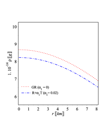
(a)  The energy-density

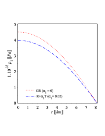
(b)  The radial pressure

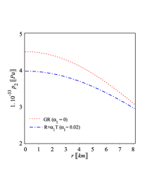
(c)  The tangential pressure

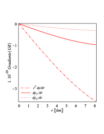
(d)  The gradients (GR)

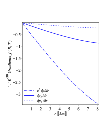
(e)  The gradients f(R,T)

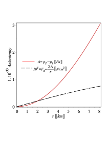
(f)  The anisotropy (GR)

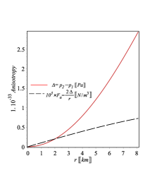
(g)  The anisotropy f(R,T)

Figure 1: The behaviors of the components of the energy-tensor of Eqs. (3), after using Eq. (13) and (17), of the pulsar HerX1 are depicted in Figs. 0(a)–0(c). The derivatives of the energy-momentum components are depicted in Figs. 0(d) and 0(e) for $f(R,T)$ and GR. Figures 0(f) and 0(g) represent the behavior of the anisotropy function $\Delta$ for GR and $f(R,T)$ cases which are given analytically by Eq. (15). All the plots displayed in Fig. 1 ensure that conditions listed from (1) to (4) are verified.

Condition (1): It is well known that any interior solution must have a regular behavior, thus the components of the energy-momentum of the fluid under consideration must be regular at the center of the star and behave regularly everywhere inside the stellar. Moreover, such physical quantities should have maximum values at the center of the star and behave in a decreasing way towards the boundary of the stellar as shown in Fig.1 0(a)–0(c).

Condition (2): The components of the energy momentum tensor in the star ($0<r<\textbf{L}$), must be non-negative, namely ${\mathrm{\rho}(0<r<\textbf{L})>0}$, ${\mathrm{p}_{1}(0<r<\textbf{L})>}0$ and ${\mathrm{p}_{2}(0<r<\textbf{L})>0}$.

Condition (3): The pressure in the radial direction of the fluid must have zero value at the boundary of the star, i.e. ${\mathrm{p}_{1}(r=\textbf{L})=0}$. On the contrary, the pressure in the tangential direction is not necessarily to be zero at the boundary of the star.

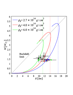
(b)  Figure of Mass and Radius relation

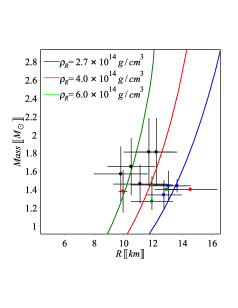
(c)  LIGO-Virgo and NICER restrictions

Figure 10: 9(a) The curves depicting the relationship between compactness and radius for different surface energy densities demonstrate that the maximal compactness is $0.92$, slightly surpassing the Buchdahl limit of $8/9$. 9(b) The curves representing the relationship between mass and radius reveal that the diagonal dashed line, representing the DEC (diagonal excluded curve), corresponds to an upper mass limit of $M\approx 5.25M_{\odot}$ within the smaller mass, with a radius of $\textbf{L}\approx 16.6$ km. This limit is established when the surface energy density is set to the saturation nuclear density of $\rho_{{nuc}}=2.7\times 10^{14}$ g/cm³. The low-mass X-ray binaries are denoted by solid blue circles, the millisecond pulsars (MSPs) are represented by solid green circles, and the gravitational wave (GW) signals are depicted by solid red circles, as indicated in Table 1. 9(c)Upon closer examination of several intriguing pulsars, it is observed that the LIGO-Virgo restrictions on the radius, the NICER restrictions on $PSRJ0030+0451$, and the combined NICER+XMM constraints on $PSRJ0740+6620$ are consistent with the $\rho_{nuc}$-curve.

Conditions from (1)–(3) are verified for the pulsar ${\textit{H}erX1}$ as indicated in Fig. 10(a)–0(e).

As shown in Fig. 1 0(a) that the model being considered provides an estimation of the core density of NS as ${\mathrm{\rho}_{core}\approx 8.2\times 10^{14}>}$ g/cm${}^{3}\approx 3.1\rho_{nuc}$ for the pulsar ${\textit{H}erX1}$. This implies that the model being studied does not rule out the likelihood of the pulsar’s core being composed of neutrons. Moreover, this value of the density (at the core) makes the assumption of the anisotropy form of the fluid to be a logic one.

Condition (4): The anisotropy function $\Delta$ should have a zero value at the core namely ${\mathrm{p}_{1}(r=0)=p_{2}(r=0)}$, and growing in the direction of the surface, i.e. $\Delta^{\prime}(0\leq r\leq\textbf{L})>0$. Therefore, the anisotropic force ${\mathit{F}_{a}=\frac{2\Delta}{r}}$ must have a zero value at the center. As Eq. (15) shows that the limit $r\to 0$ yields $\Delta\to 0$.

As shown in Fig. 1 0(f) and 10(g) that condition (4) is satisfied for the pulsar ${\textit{H}erX1}$.

Moreover, one can show that the anisotropy function ${\mathrm{\Delta}(r>0)>}0$ which means that $\mathrm{p_{2}>p_{1}}$. This condition is essential to ensure that the anisotropy force acts as a repulsive force, thereby enabling a larger size for the neutron star in comparison to the situation of an isotropic perfect fluid. Nevertheless, when $\alpha_{1}>0$, the level of anisotropy in $f(R,T)=R+\alpha_{1}T$ is lower compared to the case of GR.

4.2 Zeldovich condition

Condition (5): According to the study presented in (Zeldovich & Novikov, 1971), at the center of the star the radial pressure is required to be either less than or equal to the central energy density, namely

$$\mathrm{\frac{{p}_{1}(0)}{{\rho}(0)}\leq 1.}$$ (23)

We obtain the components of the energy momentum tensor at the center as:

$$\mathrm{{\rho}(r=0)=4{\frac{\left(3a_{0}+6a_{1}{a_{2}}^{2}+32a_{1}{a_{2}}^{2}\alpha_{1}+21\alpha_{1}a_{0}\right){a_{2}}^{2}}{{\textbf{L}}^{2}{\kappa}^{2}\left(1+2\alpha_{1}\right)\left(8\alpha_{1}+1\right)\left(a_{0}+2a_{1}{a_{2}}^{2}\right){c}^{2}}}}\,,$$

$$\mathrm{p_{1}(r=0)={\frac{12a_{2}^{2}\alpha_{1}a_{0}-8a_{1}a_{2}^{4}}{{\textbf{L}}^{2}{\kappa}^{2}\left(10\alpha_{1}+1+16\alpha_{1}{}^{2}\right)\left(a_{0}+2a_{1}a_{2}^{2}\right)}}={p}_{2}(r=0)}.\quad$$ (24)

For the pulsar ${\textit{H}erX1}$ we calculate the compactness $C=0.3100165206+\pm 0.0547087977$. Therefore, by applying the Zeldovich condition (23), we can establish a valid range for the parameter $\alpha_{1}$ as $0\leq\alpha_{1}\leq 0.02$, with the understanding that as $\alpha_{1}$ approaches zero, it is expected to converge to the GR version.

4.3 The radius and mass observational limits using pulsar ${\textit{H}erX1}$

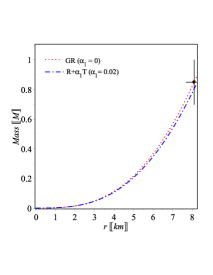
(a)  The Mass function

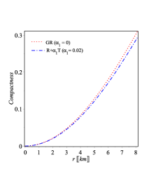
(b)  The Compactness parameter

Figure 2: The figures of the mass function (18) and compactness parameter (21) for the pulsar ${\textit{H}erX1}$. The curves are in good consistent with the observational data ($M=0.85\pm 0.15M_{\odot}$ and $\textbf{L}=8.1\pm 0.41$ km) (Legred et al., 2021). For the case $f(R,T)=R+\alpha_{1}\,T$ we employ {$\alpha_{1}=0.02$, $\kappa=2.302\times 10^{-43}\,N^{-1}$, $C=0.3100165206$, $a_{0}=0.2966665917$, $a_{1}=-0.175664532$, $a_{2}=0.2976552341$} and for the case of GR we put ($\alpha_{1}=0$) and their corresponding values are { $a_{0}=0.3100165210$, $a_{1}=-0.258327738$}.

Taking into account the limitations on the mass and radius of the pulsar ${\textit{H}erX1}$, the mass function (18) approximates $M=0.85M_{\odot}$ at $\textbf{L}=8.1$ km with a compactness $C=0.3100165206$ in consistent with the observed value, ($M=0.85\pm 0.15M_{\odot}$ and $\textbf{L}=8.1\pm 0.41$ km) (Legred et al., 2021), when we choose $\alpha_{1}$ parameter $\alpha_{1}=0.02$. This fixes the set of constants presented in Eq. (A) of Appendix A { $a_{0}=0.2966665917$, $a_{1}=-0.175664532$, $a_{2}=0.2976552341$,$\kappa=2.302\times 10^{-43}\,N^{-1}$}. These numerical values clearly verify the Zeldovich condition (23). We depict the patterns of the mass function and compactness parameter in Fig. 2 1(a) and 1(b) to illustrate the concurrence between the anticipated mass-radius relationship of the pulsar ${\textit{H}erX1}$ and the observed measurements. Comparison with GR prediction, $f(R,T)=R+\alpha_{1}\,T$ with positive value of the dimensional parameter $\alpha_{1}$ predicts same mass like the GR however, within a star of greater size (or reduced mass at equivalent size). Hence, the model $f(R,T)=R+\alpha_{1},T$ predicts a lower compactness value compared to GR for a given mass. This implies that the function $f(R,T)=R+\alpha_{1},T$ can handle greater masses or, in other words, higher levels of compactness while still maintaining stability requirements.

4.4 Geometric sector

Condition (6):In the interior region of the stellar object, ranging from $0$ to L, it is essential that the geometric sector, specifically the metric potentials ${\textit{g}_{tt}}$ and ${\textit{g}_{rr}}$, do not exhibit any coordinate or physical singularities. Clearly, the metric (9) verifies these conditions since at the core, ${\mathrm{g}_{tt}(r=0)=-\frac{\left(a_{0}+2\,a_{1}\,{a_{2}}^{2}\right)^{2}}{16{a_{2}}^{4}}}$ and ${\mathrm{g}_{rr}(r=0)=1}$, and both are well defined in the interior of the stellar $0\leq r/\textbf{L}\leq 1$.

Condition (7): The interior and the exterior solution of the metric potentials must match smoothly at the surface of the star.

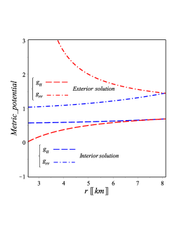
Figure 3: Inside the pulsar ${\textit{H}erX1}$, the metric potentials $g_{00}$ and $g_{rr}$ have finite values, and they seamlessly align with the Schwarzschild exterior vacuum solution. The graph guarantees the fulfillment of conditions (6) and (7).

Clearly conditions (6) and (7) are verified for the pulsar ${\textit{H}erX1}$ as indicated in Fig. 3.

Condition (8): The red-shift of the metric potential (9) is defined as:

$$Z=\frac{1}{\sqrt{-g_{tt}}}-1=\frac{1}{\sqrt{\frac{\left(a_{0}\,{\textbf{L}}^{2}+2\,a_{1}\,{a_{2}}^{2}{\textbf{L}}^{2}-2\,a_{1}\,{a_{2}}^{4}{r}^{2}\right)^{2}}{16\left(\textbf{L}^{2}-a_{2}{}^{2}\,r^{2}\right)^{2}{a_{2}}^{4}}}}-1.$$ (25)

It is known that the gravitational red-shift should be positive and has a finite value everywhere within the interior of the stellar and decreases monotonically in the direction of the surface, namely, $Z^{\prime}<0$ and $Z>0$.

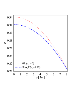
Figure 4: The red-shift function (25) of the pulsar ${\textit{H}erX1}$. Fig. 4 ensures that condition (8) is verified.

Clearly condition (8) is verified as displayed in Fig. 4.

At the center of the star, the value of $Z(0)$ is approximately $0.3326085846$, which is lower than the corresponding value in GR ($Z(0)\approx 0.3390521449$). However, at the boundary, $Z_{\textbf{L}}$ is approximately $0.2038729440$, which is similar to the GR value. Notably, this value of $Z_{\textbf{L}}$ remains below the upper red-shift limit of $Z_{\textbf{L}}=2$, as derived by Buchdahl (1959) (Buchdahl, 1959). For further exploration of the anisotropic nature, one can refer to studies by Ivanov and Sibgatullin (2002) (Ivanov, 2002) and Barraco et al. (2003) (Barraco et al., 2003), as well as the study by Boehmer et al. (2006) that includes a cosmological constant (Böhmer & Harko, 2006). We observe that the maximum red-shift limit is not a highly restrictive condition, and therefore it does not provide a suitable means to determine a maximum limit on the compactness, as previously discussed in works such as those by (c.f., Ivanov, 2002; Barraco et al., 2003; Böhmer & Harko, 2006). Nevertheless, the scenario shifts when the energy conditions related to the matter configuration are taken into account, imposing more stringent limitations. This was demonstrated in the investigation conducted by Roupas (2020) (Roupas & Nashed, 2020).

4.5 The energy conditions

The focusing theorem within the framework of GR states that in the Raychaudhuri equation, the trace of the tidal tensor, given by ${\mathrm{R}{\alpha\beta}u^{\alpha}u^{\beta}\geq 0}$ and ${\mathrm{R}{\alpha\beta}\ell^{\alpha}\ell^{\beta}\geq 0}$, is always positive. Here, ${\mathrm{u}^{\alpha}}$ represents any arbitrary timelike vector, and ${\mathrm{\ell}^{\alpha}}$ represents null vector. This gives rise to four energy conditions that impose constraints on ${\mathrm{\mathbb{missing}}{T}^{\alpha\beta}}$, which are applicable not only in the context of General Relativity but can also be extended to modified gravitational theories. Specifically, in the case of $f(R,T)=R+\alpha_{1}T$ gravity, these energy conditions can be reformulated in terms of the energy-momentum tensor. ${\mathrm{{T}}{{}^{\alpha}}{{}_{\beta}}}=\mathrm{diag(-\rho c^{2},p_{1},p_{2},p_{2})}$, since ${\mathrm{\mathbb{missing}}{R}_{\alpha\beta}=\kappa\left({{T}}_{\alpha\beta}-\frac{1}{2}g_{\alpha\beta}{{T}}\right)}$.

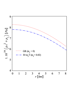
(a) WEC & NEW (radial)

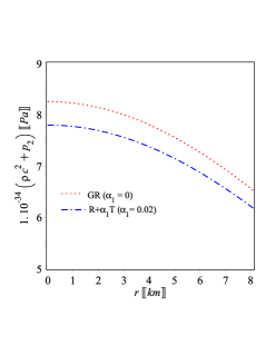
(b) WEC &NEC (tangential)

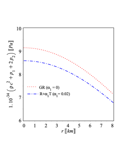
(c) SEC

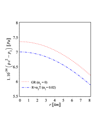
(d)  DEC (radial)

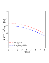
(e)  DEC (tangential)

Figure 5: The characteristics of energy conditions when considering Eq. (3) of the pulsar ${\textit{H}erX1}$. The plots of Fig. 5 ensures that all the energy conditions (9) are satisfied.

Condition (9): Any physically acceptable stellar model must be compatible with the energy conditions:

• The null energy condition (NEC) which should satisfy the following identities: ${\mathrm{\rho}c^{2}+p_{1}\geq 0}$,   ${\mathrm{\rho}c^{2}+p_{2}\geq 0}$ ,

• The weak energy condition (WEC) which should satisfy the following identities: ${\mathrm{\rho}\geq 0}$,  ${\mathrm{\rho}c^{2}+p_{1}>0}$,  ${\mathrm{\rho}c^{2}+p_{2}>0}$ ,

• The dominant energy conditions (DEC) which should satisfy the following identities: ${\mathrm{\rho}\geq 0}$,  ${\mathrm{\rho}c^{2}-p_{1}\geq 0}$, and ${\mathrm{\rho}c^{2}-p_{2}\geq 0}$ ,

• The strong energy condition (SEC) which should satisfy the following identities: ${\mathrm{\rho}c^{2}+p_{1}+2p_{2}\geq 0}$,  ${\mathrm{\rho}c^{2}+p_{1}\geq 0}$,  ${\mathrm{\rho}c^{2}+p_{2}\geq 0}$ .
  

Now let us rewrite the field equations (LABEL:eq:Feqs) as:

$${\mathrm{\rho}c^{2}} = {\mathrm{\rho}_{GR}c^{2}+\frac{5\alpha_{1}}{3(1+3\,\alpha_{1})}\left(p_{1}+2\,p_{2}\right)},$$

$${\mathrm{p}_{1}} = {\mathrm{p_{1}}_{GR}+\frac{\alpha_{1}}{3+11\alpha_{1}}\left(3\rho c^{2}-10p_{2}\right)},$$

$${\mathrm{p}_{2}} = {\mathrm{p_{2}}_{GR}+\frac{3\alpha_{1}}{3+16\,\alpha_{1}}\left(\rho c^{2}-\frac{5}{3}p_{1}\right)}\,.$$ (26)

When $\alpha_{1}=0$ one can derive the GR case. Now let us discuss condition (9) analytically. Equation (4.5) shows clearly that the effect of the coupling constant which is a small effect as shown in Fig. 54(a)–4(e)

Using conditions (1) and (2), it can be demonstrated that both the density and pressures within the star are consistently positive which means that the NEC is verified. Moreover, we can show that:

$${\mathrm{\rho}c^{2}}+{\mathrm{p}_{1}}=({\mathrm{\rho}_{GR}c^{2}}+{\mathrm{p_{1}}_{GR}})+{\mathrm{\alpha}_{1}}\frac{\left(27\,{\alpha_{1}}+9\,\right){\mathrm{\rho}c^{2}}+\left(55\,{\alpha_{1}}+15\,\right){\mathrm{p}_{1}}+20\,{\mathrm{\alpha_{1}}}{\mathrm{p}_{2}}}{9+99\,{\alpha}^{2}+60\,\alpha},$$

$${\mathrm{\rho}c^{2}}+{\mathrm{p}_{2}}=({\mathrm{\rho}_{GR}c^{2}}+{\mathrm{p_{2}}_{GR}})-\frac{\alpha_{1}\,\left(10{\mathrm{p}_{2}}[3-16\alpha_{1}]-125\,{\mathrm{p}_{1}}\alpha_{1}+9\,{\mathrm{\rho}}c^{2}[1+3\alpha_{1}]\right)}{3\left(1+3\,\alpha_{1}\right)\left(3-16\,\alpha\right)},$$

$${\mathrm{\rho}}c^{2}+{\mathrm{p}_{1}}+2{\mathrm{p}_{2}}=({\mathrm{\rho}_{GR}}c^{2}+{\mathrm{p_{1}}{{}_{G}R}}+2{\mathrm{p_{2}}_{GR}})$$

$$+{\frac{\alpha_{1}\left(162\,{\alpha_{1}}^{2}+297{\alpha_{1}}+81\right){\mathrm{\rho}c^{2}}-\alpha_{1}\left(1870{\alpha_{1}}^{2}+675{\alpha_{1}}+45\right){\mathrm{p}_{1}}+20{\mathrm{p}_{2}}{\alpha_{1}}^{2}\left(3-16\alpha_{1}\right)}{27-1584\,{\alpha_{1}}^{3}-663\,{\alpha_{1}}^{2}+36\,\alpha_{1}}},$$ (27)

$${\mathrm{\rho}c^{2}}-{\mathrm{p}_{1}}=({\mathrm{\rho}_{GR}c^{2}}-{\mathrm{p_{1}}_{GR}})+\frac{\alpha_{1}\,\left(15\,{\mathrm{p}_{1}}+55{\mathrm{p}_{1}}\alpha_{1}+60\,p_{2}+200\,{\mathrm{p}_{2}}\alpha_{1}-9\,{\mathrm{\rho}}c^{2}[1+3\alpha_{1}]\right)}{3\left(1+3\,\alpha_{1}\right)\left(3+11\,\alpha_{1}\right)},$$

$${\mathrm{\rho}c^{2}}-{\mathrm{p}_{2}}=({\mathrm{\rho}_{GR}c^{2}}-{\mathrm{p_{2}}_{GR}})+{\frac{\alpha_{1}\left({\mathrm{p}_{1}}[30-35\alpha_{1}]+{\mathrm{p}_{2}}[30-160{\mathrm{p}_{2}}\alpha_{1}]-9{\mathrm{\rho}c^{2}}[1+\alpha_{1}]\right)}{9-144{\alpha_{1}}^{2}-21\,\alpha_{1}}},$$

$${\mathrm{\rho}c^{2}}-{\mathrm{p}_{1}}-2{\mathrm{p}_{2}}=({\mathrm{\rho}_{GR}c^{2}}-{\mathrm{p_{1}}{{}_{G}R}}-2{\mathrm{p_{2}}_{GR}})$$ (28)

$$+\frac{\alpha_{1}\left({\mathrm{p}_{1}}[135+525\alpha_{1}+110{\alpha_{1}}^{2}]+{\mathrm{p}_{2}}[180-360\alpha_{1}-3200\,{\alpha_{1}}^{2}]-3\,{\mathrm{\rho}c^{2}}[27+99\alpha_{1}+54{\alpha}^{2}]\right)}{3\left(1+3\,\alpha_{1}\right)\left(3+11\,\alpha_{1}\right)\left(3-16\,\alpha_{1}\right)}.\qquad$$ (29)

Since $\alpha_{1}>0$ (in this study $\alpha_{1}=0.02$) in addition to the fact that ${\mathrm{p}_{r}\geq 0}$, ${\mathrm{p}_{t}\geq 0}$, and ${\mathrm{\rho}\geq 0}$; it is still necessary to demonstrate that

$${\mathrm{p}_{1}}[30-35\alpha_{1}]+{\mathrm{p}_{2}}[30-160p_{2}\alpha_{1}]>9\,{\mathrm{\rho}c^{2}}[1+\alpha_{1}]>0\,,$$

$$\left(162\,{\alpha_{1}}^{2}+297{\alpha_{1}}+81\right){\mathrm{\rho}c^{2}}+20{\mathrm{p}_{2}}{\alpha_{1}}\left(3-16\alpha_{1}\right)>\left(1870{\alpha_{1}}^{2}+675{\alpha_{1}}+45\right)p_{1}>0\,,$$

and

$$10{\mathrm{p}_{2}}[3-16\alpha_{1}]+9{\mathrm{\rho}c^{2}}[1+3\alpha_{1}]>125\,{\mathrm{p}_{1}}\alpha_{1}>0\,,$$

to ensure that the energy conditions are satisfied (1–4).

Clearly the energy conditions (9) are verified for the pulsar ${\textit{H}erX1}$ as shown in Fig. 54(a)–4(e).

Lastly, we observe that the density prevails over the radial and tangential pressures is ensured in $f(R,T)=R+\alpha_{1}T$ as far as it is satisfied in GR, because

$${\mathrm{\rho}c^{2}}-\mathrm{p_{1}}-2\mathrm{p_{2}}=\frac{\alpha_{1}\left({\mathrm{p}_{1}}[135+525\alpha_{1}+110{\alpha_{1}}^{2}]+p_{2}[180-360\alpha_{1}-3200\,{\alpha_{1}}^{2}]-3\,{\mathrm{\rho}c^{2}}[27+99\alpha_{1}+54{\alpha}^{2}]\right)}{3\left(1+3\,\alpha_{1}\right)\left(3+11\,\alpha_{1}\right)\left(3-16\,\alpha_{1}\right)}.$$

The above condition is commonly mentioned as the strong energy condition by certain researchers (c.f. Kolassis et al., 1988; Ivanov, 2017; Das et al., 2019b; Roupas & Nashed, 2020).

Based on the aforementioned discussion, we can demonstrate a strong connection between the energy conditions and the matter fluid in $f(R,T)$ gravity.

4.6 Stability conditions and causality

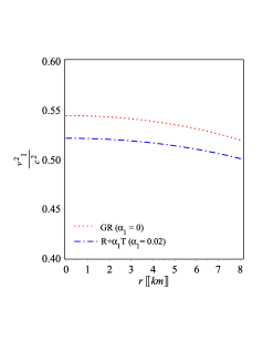
(a)  Radial speed of sound

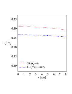
(b)  Tangential speed of sound

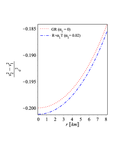
(c)  difference between radial and tangential speed of sounds

Figure 6: Tangential and radial sound speeds (30) of ${\textit{H}erX1}$ ensure that the causality and stability conditions (10) and (11) are met.

The radial and tangential speeds of sound are defined as (Herrera, 1992; Abreu et al., 2007):

$${\mathrm{v}_{1}^{2}}=\frac{d{\mathrm{p}}_{1}}{d{\mathrm{\rho}}}=\frac{{\mathrm{p}^{\prime}}_{1}}{{\mathrm{\rho}^{\prime}}}\,,\quad{\mathrm{v}_{2}^{2}}=\frac{d{\mathrm{p}}_{2}}{d{\mathrm{\rho}}}=\frac{{\mathrm{p}^{\prime}}_{2}}{{\mathrm{\rho}^{\prime}}}\,,$$ (30)

where the energy density and the derivative of the pressures are given by Eqs. (B)–(B).

Condition (10): The star’s structure must adhere to causality, meaning it must meet the condition that sound speeds are positive and less than unity within the star ($0\leq\frac{{\mathrm{v}_{1}}}{c}\leq 1$, $0\leq\frac{{\mathrm{v}_{2}}}{c}\leq 1$), and they should decrease monotonically towards the surface ($({\mathrm{v}^{\prime}_{1}})^{2}<0$, $({\mathrm{v}^{\prime}_{2}})^{2}<0$).

Condition (11): For the star to be stable, its structure must fulfill the stability condition $-1<\frac{{\mathrm{v}_{t}^{2}}-{\mathrm{v}_{r}^{2}}}{c^{2}}<0$ throughout the entire star (Herrera, 1992).

The causality and stability conditions, as stated in equations (10) and (11), are clearly satisfied for the pulsar ${\textit{H}erX1}$, as depicted in Fig. 65(a)–5(c).

4.7 The adiabatic and hydrodynamic equilibrium conditions

In order to validate the reliability of the considered model, we conduct two additional tests to assess the stability of the obtained model in $f(R,T)=R+\alpha_{1}T$ gravity. Initially, we examine the adiabatic indices of a spacetime having spherical symmetric. These indices, that determine the ratio of specific heats, are analyzed to assess the stability of the model (Chandrasekhar, 1964; Chan et al., 1993) as:

$${\mathrm{\gamma}}=\frac{4}{3}\left(1+\frac{{\mathrm{\Delta}}}{|{\mathrm{p}}^{\prime}_{1}|}\right)_{max}\,,\qquad\quad{\mathrm{\Gamma}_{1}}=\frac{{\mathrm{\rho}c^{2}}+{\mathrm{p}_{1}}}{{\mathrm{p}_{1}}}{\mathrm{v}_{1}^{2}}\,,\qquad\quad{\mathrm{\Gamma}_{2}}=\frac{{\mathrm{\rho}c^{2}}+{\mathrm{p}_{2}}}{{\mathrm{p}_{2}}}{\mathrm{v}_{2}^{2}.}$$ (31)

In the case of an anisotropic fluid, the stability of the sphere is guaranteed when ${\mathrm{\Gamma}}={\mathrm{\gamma}}$ (or when ${\mathrm{\Gamma}}>{\mathrm{\gamma}}$), as discussed in the work by Chan and Santos (Chan et al., 1993, see). Clearly, in the case where ${\mathrm{\gamma}}=4/3$ and ${\mathrm{\Gamma}_{1}}={\mathrm{\Gamma}_{2}}$, the adiabatic lead to an isotropic sphere, as indicated by the research conducted by Harrison (Heintzmann & Hillebrandt, 1975).

Next, we consider the truth of the TOV equation (Hansraj & Banerjee, 2018; Oppenheimer & Volkoff, 1939) by considering the assumption of hydrostatic equilibrium in the star. The TOV equation has been modified to incorporate the newly introduced force of $f(R,T)=R+\alpha_{1}T$ term, and is denoted as $F_{T}$. It can be rewritten as follows:

$${\mathit{F}_{a}}+{\mathit{F}_{g}}+{\mathit{F}_{h}}+{\mathit{F}_{T}=0}\,.$$ (32)

Here ${\mathrm{F}_{h}}$ and ${\mathrm{F}_{g}}$ are the hydrostatic and the gravitational forces. We defined the different forces as (Nashed & El Hanafy, 2022; El Hanafy, 2022):

$${\mathrm{F}_{a}}= \frac{2{\mathrm{\Delta}}}{\mathrm{r}},\qquad{\mathrm{F}_{g}}=-\frac{{\mathrm{M}_{g}}}{r}({\mathrm{\rho}c^{2}}+{\mathrm{p}_{1}})e^{{\mathrm{\gamma}/2}},\qquad$$

$${\mathrm{F}_{h}}= -{\mathrm{p}^{\prime}_{1}},\qquad{\mathrm{F}_{T}}=\frac{\alpha_{1}}{3(1-\alpha_{1})}({\mathrm{c}^{2}\rho}^{\prime}-{\mathrm{p}}^{\prime}_{1}-2{\mathrm{p}}^{\prime}_{2}),$$ (33)

where ${\mathrm{\gamma}}\equiv{\mathrm{\gamma}}(r)=\mu-\nu$ and the mass (energy) ${\mathrm{M}_{g}}$ of an isolated systems is given by (Tolman, 1930)

$${\mathrm{M}_{g}(r)} = {\int_{\mathrm{V}}}\Big{(}\mathbb{{\mathrm{T}}}{{}^{r}}{{}_{r}}+\mathbb{{\mathrm{T}}}{{}^{\theta}}{{}_{\theta}}+\mathrm{T}{{}^{\phi}}{{}_{\phi}}-\mathrm{T}{{}^{t}}{{}_{t}}\Big{)}\sqrt{-g}\,dV$$ (34)

$$= \frac{(e^{\mu/2})^{\prime}}{e^{\mu}}e^{\nu/2}r=\frac{\mu^{\prime}}{2}re^{-\gamma/2}\,.$$

Here, ${\mathrm{F}_{g}}$ represents the gravitational force, which can be defined as $-\frac{a_{0}r}{\textbf{L}^{2}}({\mathrm{\rho}c^{2}}+{\mathrm{p}_{1}})$. We now incorporate the stability conditions associated with the relativistic modified TOV equation and adiabatic indices.

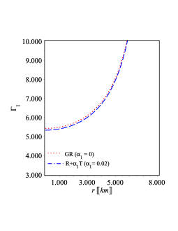
(a)  Radial adiabatic index

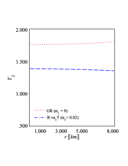
(b)  Tangential adiabatic index

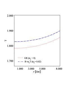
(c)  The adiabatic index

Figure 7: The adiabatic indices given by Eq. (31) of the pulsar ${\textit{H}erX1}$. The graphs provide confirmation that the stability conditions (12) hold true throughout the pulsar.

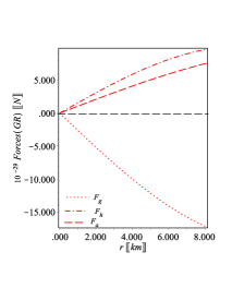
(a)  GR

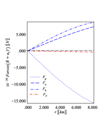
(b)  $f(R,T)=R+\alpha_{1}\,T$

Figure 8: The different forces (4.7) of the amended TOV equation (32) of the pulsar ${\textit{H}erX1}$. The plots ensure the stability condition (13) which is verified for ${\textit{H}erX1}$ .

Condition (12): The anisotropic star model maintains a stable behavior since the adiabatic indices verify ${\mathrm{\Gamma}_{t}}>{\mathrm{\gamma}}$ and ${\mathrm{\Gamma}_{r}}>{\mathrm{\gamma}}$ throughout the entire pulsar. By employing the pressures and density described in Eqs. (3), along with their derivatives (B)–(B), we illustrate the adiabatic (31) of the pulsar ${\textit{H}erX1}$ for both the $f(R,T)$ and GR as shown in Figure 7.

The stability conditions and adiabatic indices of condition (12) are evidently satisfied for the pulsar ${\textit{H}erX1}$, as illustrated in Figure 7.

Condition (13): The anisotropic star achieves a state of hydrodynamic equilibrium, as the forces verify the TOV equation (32). Utilizing Eqs. (3) and (B)–(B), we calculate the forces (4.7), which are illustrated in Figure 8 for both the general relativity (GR) and $f(R,T)$ cases. The figures clearly demonstrate that the negative force counterbalances the positive ones, resulting in hydrodynamic equilibrium and supporting the requirement for a stable configuration.

The condition of hydrodynamic equilibrium (13) is evidently satisfied for the pulsar ${\textit{H}erX1}$, as depicted in Figure 8..

4.8 EoS

By utilizing the observational data from the pulsar ${\textit{H}erX1}$, we were able to determine a reasonable value for the parameter $\alpha_{1}=0.02$. Consequently, we compute the surface density, which has been determined to be approximately $\rho_{R}\approx 6.5\times 10^{14}$ g/cm³, while at the core, the density increases to approximately $\rho_{core}\approx 8.2\times 10^{14}$ g/cm³. It is worth mentioning that the central density in $f(R,T)$ gravity with $\alpha_{1}>0$ is lower than the corresponding value in general relativity (GR) ($\alpha_{1}=0$). This is due to the fact that within a given radius, the estimated mass in $f(R,T)$ gravity is lower than that in Einstein gravity, as illustrated in Figure 2 1(a). The value of the central density implies that the core of ${\textit{H}erX1}$ is composed of neutrons.

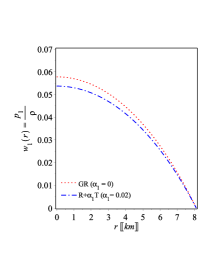
(a)  Radial EoS

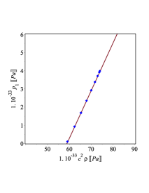
(b)  Linear radial EoS

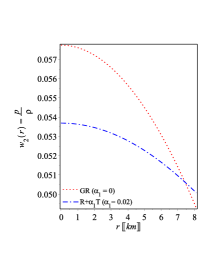
(c)  Tangential EoS

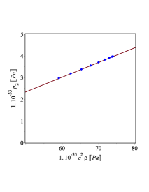
(d)  Linear tangential EoS

Figure 9: The relationship between pressures and density in the pulsar ${\textit{H}erX1}$ aligns well with a linear equation of state (EoS) incorporating a bag constant. The slopes $dp_{1}/d\rho=0.27c^{2}$ and $dp_{2}/d\rho=0.068c^{2}$ provide clear evidence that the matter within the neutron star adheres to the proposed conformal bound on the sound speed, $c_{s}^{2}\leq c^{2}/3$, throughout the star’s interior.

demonstrate the equation of state (EoS) parameters that exhibits slightly variation from their maximum values at the center, gradually decreasing in a monotonic manner towards the surface. At the boundary, it is expected that the parameter $w_{1}$ approaches zero, aligning with the anticipated behavior. In Figs. 98(a) and 8(c), we plot EoS, i.e. we plot $\mathrm{w_{1}=p_{1}/\rho}$ and $\mathrm{w_{2}=p_{2}/\rho}$, when the dimensionless parameter $\alpha_{1}=0$ which is the GR case, and $\alpha_{1}\neq 0$. The plots, Figs. 98(a) and 8(c), demonstrate the equation of state (EoS) parameters that exhibits slightly variation from their maximum values at the center, gradually decreasing in a monotonic manner towards the surface. At the boundary, it is expected that the parameter $w_{1}$ approaches zero, aligning with the anticipated behavior. It is important to acknowledge that the changes in the equation of state (EoS) parameters are more constrained in the context of $R+\alpha_{1}T$ compared to the case of GR. Moreover, we stress that we have not assume any formula of the EoS in the model under consideration, 98(a) and 8(c). Nevertheless, we demonstrate that EoS $p(\rho)$ of the radial and tangential directions can be accurately approximated by linear relationships. For the pulsar ${\textit{H}erX1}$, the best-fit equations are found to be $p_{1}\approx 0.262,\rho-15.47$ and $p_{2}=0.06799,\rho-1.0623$. More interestingly, the slopes of the fitted lines $dp_{1}/d\rho=0.262=v_{1}^{2}$ and $dp_{2}/d\rho=0.06799=v_{2}^{2}$ are in agreement with the numerical values listed in Table 3 for the model of the present study.

5 Additional Observational Constraints

Next, we will compare the model being considered with data from other pulsars in order to assess its validity across a broad range of astrophysical observations. Additionally, we generate a mass-radius profile by considering different boundary densities that align with the nuclear saturation density. This analysis reveals the model’s consistency in predicting masses within the lower mass range of 3.5 to 5.3 times the mass of the Sun ($M_{\odot}$), often referred to as the “mass gap.” Furthermore, we compare the compactness of the present study with the Buchdahl one bound.

5.1 Stars data

In addition to the analysis conducted on the pulsar ${\textit{H}erX-1}$, the same methodology is applied to twenty-two other stars, spanning a range from 0.8 times the mass of the Sun ($M_{\odot}$) to heavy pulsars with a mass of 2.01 times $M_{\odot}$. Table 1, presents the observed radii and masses of each pulsar, along with the respective model parameters $a_{0}$, $a_{1}$, $a_{2}$, assuming a value of $\alpha_{1}=0.2$ for the $f(R,T)$ parameter. The results demonstrate that the model proposed in this study successfully predicts masses for these pulsars that are consistent to the observed ones. Table 3, displays the evaluated values of various important physical quantities. As indicated in Table 2, the density values obtained are in accordance with the expected nuclear density. It is important to emphasize that this study does not rely on any specific form of equations of state (EoSs). The obtained results are found to align well with a linear behavior, with the slopes $dp_{r}/d\rho$ and $dp_{t}/d\rho$ of the best-fit lines being in agreement. Furthermore, the values presented in Table 3 ensure stablity and causality, satisfying all the necessary physical conditions discussed in Section 4.1.In addition, we provide the predicted boundary redshift numerical; values for the twenty-two pulsars based on the current model. It is noteworthy that all of these values adhere to the upper bound limit of $Z_{\textbf{L}}\leq 2$ proposed by Buchdahl (Buchdahl, 1959). This consistency also holds true for anisotropic spheres (Ivanov, 2002; Barraco et al., 2003).

Table 1: The mass-radius of twenty two stars with their corresponding parameters ($\alpha_{1}=0.02$).

Pulsar	Ref.	observed mass ($M_{\odot}$)	obs. radius [km]	estimated mass ($M_{\odot}$)	$a_{0}$	$a_{1}$	$a_{2}$
Her X-1	(Abubekerov et al., 2008)	$0.85\pm 0.15$	$8.1\pm 0.41$	$0.905$	$0.297$	$-0.176$	$0.298$
M13	(Webb & Barret, 2007)	$1.38\pm 0.2$	$9.95\pm 0.27$	$1.459$	$0.394$	$-0.285$	$0.351$
RX J185635-3754	(Pons et al., 2002)	$0.9\pm 0.2$	$6$	$0.949$	$0.427$	$-0.324$	$0.369$
GW170817-2	(Abbott et al., 2018b)	$1.27\pm 0.09$	$11.9\pm 1.4$	$1.351$	$0.302$	$-0.181$	$0.301$
EXO 1785-248	(Özel et al., 2009)	$1.3\pm 0.2$	$8.849\pm 0.4$	$1.372$	$0.418$	$-0.313$	$0.364$
PSR J0740+6620	(Raaijmakers et al., 2019)	$1.34\pm 0.16$	$12.71\pm 1.19$	$1.426$	$0.298$	$-0.177$	$0.298$
LIGO	(Abbott et al., 2020b)	$1.4$	$12.9\pm 0.8$	$1.489$	$0.307$	$-0.187$	$0.303$
X7	(Heinke et al., 2006)	$1.4$	$14.5\pm 1.8$	$1.492$	$0.340$	$-0.607$	$0.284$
PSR J0037-4715	(Reardon et al., 2016)	$1.44\pm 0.07$	$13.6\pm 0.9$	$1.532$	$0.299$	$-0.179$	$0.299$
LMC X-4	(Rawls et al., 2011)	$1.04\pm 0.09$	$8.301\pm 0.2$	$1.103$	$0.355$	$-0.240$	$0.330$
PSR J0740+6620	(Miller et al., 2019)	$1.44\pm 0.16$	$13.02\pm 1.24$	$1.531$	$0.312$	$-0.193$	$0.307$
Cen X-3	(Naik et al., 2011)	$1.49\pm 0.49$	$9.178\pm 0.13$	$1.566$	$0.464$	$-0.369$	$0.388$
GW170817-1	(Abbott et al., 2018b)	$1.45\pm 0.09$	$11.9\pm 1.4$	$1.539$	$0.345$	$-0.230$	$0.325$
4U 1820-30	(Güver et al., 2010)	$1.46\pm 0.2$	$11.1\pm 1.8$	$1.546$	$0.374$	$-0.261$	$0.340$
4U 1608-52	(Marshall & Angelini, 1996)	$1.57\pm 0.3$	$9.8\pm 1.8$	$1.651$	$0.457$	$-0.361$	$0.385$
KS 1731-260	(Özel et al., 2009)	$1.61\pm 0.37$	$10\pm 2.2$	$1.692$	$0.460$	$-0.364$	$0.386$
EXO 1745-268	(Özel et al., 2009)	$1.65\pm 0.25$	$10.5\pm 1.8$	$1.736$	$0.448$	$-0.35$	$0.380$
Vela X-1	(Rawls et al., 2011)	$1.77\pm 0.08$	$9.56\pm 0.08$	$1.845$	$0.531$	$-0.456$	$0.424$
4U 1724-207	(Özel et al., 2009)	$1.81\pm 0.27$	$12.2\pm 1.4$	$1.909$	$0.423$	$-0.318$	$0.366$
SAX J1748.9-2021	(Özel et al., 2009)	$1.81\pm 0.3$	$11.7\pm 1.7$	$1.906$	$0.441$	$-0.341$	$0.376$
PSR J1614-2230	(Demorest et al., 2010)	$1.97\pm 0.04$	$13\pm 2$	$2.076$	$0.432$	$-0.32$	$0.371$
PSR J0348+0432	(Antoniadis et al., 2013)	$2.01\pm 0.04$	$13\pm 2$	$2.117$	$0.441$	$-0.341$	$0.376$

Table 2: Calculation of the most interest physical quantities.

Pulsar	$\rho(0)$	$\rho_{\textbf{L}}$	$v_{1}^{2}(0)/c^{2}$	$v_{1}^{2}(\textbf{L})/c^{2}$	$v_{2}^{2}(0)/c^{2}$	$v_{2}^{2}(\textbf{L})/c^{2}$	$\rho c^{2}-p_{1}-2p_{2}|_{0}$	$\rho-p_{1}-2p_{2}|_{\textbf{L}}$	$Z_{\textbf{L}}$
	[$g/cm^{3}$]	[$g/cm^{3}$]					[$Pa$]	[$Pa$]
Her X-1	8.23$\times 10^{14}$	6.54$\times 10^{14}$	0.262	0.25	0.068	0.064	8.59$\times 10^{34}$	6.76$\times 10^{34}$	0.204
RX J185635-3754	2.31$\times 10^{15}$	1.62$\times 10^{15}$	0.346	0.296	0.146	0.122	2.69$\times 10^{35}$	1.81$\times 10^{35}$	0.340
LMC X-4	9.67$\times 10^{14}$	7.27$\times 10^{14}$	0.3	0.269	0.998	0.878	1.05$\times 10^{35}$	7.77$\times 10^{34}$	0.260
GW170817-2	3.89$\times 10^{14}$	3.08$\times 10^{14}$	0.274	0.252	0.73	0.665	4.07$\times 10^{34}$	3.19$\times 10^{34}$	0.208
EXO 1785-248	1.04$\times 10^{15}$	7.31$\times 10^{14}$	0.34	0.293	0.14	0.117	1.19$\times 10^{35}$	8.12$\times 10^{34}$	0.329
PSR J0740+6620	3.36$\times 10^{14}$	2.67$\times 10^{14}$	0.272	0.251	0.713	0.651	3.51$\times 10^{34}$	2.76$\times 10^{34}$	0.205
M13	7.63$\times 10^{14}$	5.51$\times 10^{14}$	0.323	0.283	0.123	0.105	8.59$\times 10^{34}$	6.04$\times 10^{34}$	0.302
LIGO	3.38$\times 10^{14}$	2.66$\times 10^{14}$	0.276	0.253	0.754	0.684	3.55$\times 10^{34}$	2.76$\times 10^{34}$	0.213
X7	2.61$\times 10^{14}$	2.14$\times 10^{14}$	0.424	0.366	0.226	0.183	1.85$\times 10^{34}$	1.69$\times 10^{34}$	0.183
PSR J0037-4715	2.95$\times 10^{14}$	2.34$\times 10^{14}$	0.273	0.251	0.719	0.656	3.08$\times 10^{34}$	2.42$\times 10^{34}$	0.206
PSR J0740+6620	3.39$\times 10^{14}$	2.65$\times 10^{14}$	0.279	0.255	0.782	0.707	3.58$\times 10^{34}$	2.77$\times 10^{34}$	0.219
GW170817-1	4.55$\times 10^{14}$	3.45$\times 10^{14}$	0.295	0.265	0.944	0.836	4.92$\times 10^{34}$	3.67$\times 10^{34}$	0.250
4U 1820-30	5.74$\times 10^{14}$	4.24$\times 10^{14}$	0.311	0.275	0.11	0.095	6.35$\times 10^{34}$	4.58$\times 10^{34}$	0.279
Cen X-3	1.1$\times 10^{15}$	7.35$\times 10^{14}$	0.376	0.313	0.176	0.142	1.32$\times 10^{35}$	8.43$\times 10^{34}$	0.386
4U 1608-52	9.45$\times 10^{14}$	6.38$\times 10^{14}$	0.37	0.31	0.171	0.138	1.13$\times 10^{35}$	7.28$\times 10^{34}$	0.378
KS 1731-260	9.14$\times 10^{14}$	6.15$\times 10^{14}$	0.372	0.311	0.173	0.139	1.1$\times 10^{35}$	7.03$\times 10^{34}$	0.381
EXO 1745-268	8.03$\times 10^{14}$	5.48$\times 10^{14}$	0.362	0.306	0.163	0.133	9.53$\times 10^{34}$	6.21$\times 10^{34}$	0.366
Vela X-1	1.21$\times 10^{15}$	7.47$\times 10^{14}$	0.448	0.349	0.25	0.186	1.59$\times 10^{35}$	8.99$\times 10^{34}$	0.486
4U 1724-207	5.52$\times 10^{14}$	3.87$\times 10^{14}$	0.343	0.294	0.143	0.119	6.38$\times 10^{34}$	4.32$\times 10^{34}$	0.334
SAX J1748.9-2021	6.34$\times 10^{14}$	4.36$\times 10^{14}$	0.357	0.302	0.157	0.129	7.46$\times 10^{34}$	4.92$\times 10^{34}$	0.357
PSR J1614-2230	5.00$\times 10^{14}$	3.47$\times 10^{14}$	0.35	0.298	0.15	0.124	2.65$\times 10^{34}$	5.83$\times 10^{34}$	0.346
PSR J0348+0432	5.13$\times 10^{14}$	3.53$\times 10^{14}$	0.357	0.302	0.157	0.129	6.04$\times 10^{34}$	3.98$\times 10^{34}$	0.357

Table 3: Calculation of the adiabatic indices at the center of the stellar.

Pulsar	$\Gamma_{1}(0)$	$\Gamma_{2}(0)$	$\gamma$
Her X-1	5.34	1.39	1.83
RX J185635-3754	3.9	1.65	1.72
LMC X-4	4.54	1.51	1.78
GW170817-2	5.25	1.4	1.82
EXO 1785-248	3.96	1.63	1.73
PSR J0740+6620	5.31	1.4	1.83
M13	4.16	1.58	1.75
LIGO	5.17	1.41	1.82
X7	5.77	1.33	1.85
PSR J0037-4715	5.3	1.4	1.82
PSR J0740+6620	5.1	1.42	1.81
GW170817-1	4.66	1.49	1.79
4U 1820-30	4.35	1.54	1.76
Cen X-3	3.67	1.72	1.69
4U 1608-52	3.7	1.71	1.7
KS 1731-260	3.69	1,72	1.69
EXO 1745-268	3.76	1.69	1.7
Vela X-1	3.36	1.9	1.63
4U 1724-207	3.93	1.64	1.72
SAX J1748.9-2021	3.8	1.68	1.71
PSR J1614-2230	3.87	1.65	1.71
PSR J0348+0432	3.81	1.68	1.71

6 Mass-Radius diagram

Table 3 provides the range of surface densities as $2.14\times 10^{14}\lesssim\rho_{\textbf{L}}\lesssim 7.47\times 10^{14}$ g/cm³. Based on this information, we select three specific densities at the surface as: $\rho_{\textbf{L}}=\rho_{nuc}=2.7\times 10^{14}$ g/cm³, $\rho_{\textbf{L}}=4\times 10^{14}$ g/cm³ and $\rho_{\textbf{L}}=6\times 10^{14}$ g/cm³ to encompass the density at which nuclear solidification occurs. Next, for the dimensionless parameter $\alpha_{1}=0.02$, we establish a correlation between L and the compactness $C$ for each boundary condition. This relationship is derived by employing the density equation (3), specifically $\rho(r=\textbf{L})=\rho_{\textbf{L}}$. In Figure 109(a), we present the curves illustrating the relationship between compactness and radius, considering the selectedsurface density conditions. The plots demonstrate the maximal compactness observed is $0.92$, exceeding the limit of Buchdahl.

(a)  Figure of Compactness and Radius relation

In the following, we illustrate the mass-radius curves, accompanied by the observational data obtained in Table 1, as shown in Figure 109(b). By employing the DEC constraint, we determine that the maximal permissible mass is $M_{\text{max}}=5.25M_{\odot}$, with a corresponding maximal radius of $\textbf{L}{\text{max}}=16.6$ km. This calculation is based on the surface density at the nuclear saturation of $\rho{\text{nuc}}=2.7\times 10^{14}$ g/cm³. Significantly, within the same boundary condition, GR yields a maximal mass of $4.1M_{\odot}$ with a corresponding maximum radius of $\textbf{L}_{\text{max}}=16.8$ km. When compared to the predictions of GR, the $f(R,T)$ theory with a positive parameter $\alpha_{1}=0.02$ forecasts a mass that is nearly the same, albeit with a slightly smaller size of approximately 0.2 km. Similarly, when considering surface densities of $\rho_{\textbf{L}}=4\times 10^{14}$ g/cm³ and $\rho_{\textbf{L}}=6\times 10^{14}$ g/cm³, we determine the corresponding maximum masses and radii as follows: ($M_{\text{max}}=4.28M_{\odot},\textbf{L}{\text{max}}=13.8$ km) and ($M{\text{max}}=3.5M_{\odot},\textbf{L}_{\text{max}}=11.4$ km). These values are consistent with the nuclear solidification density. Surprisingly, the present model has the ability to produce a NS within the mass range of $3.5-5.25M_{\odot}$, which leaves open the possibility that the companion of the binary system GW190814, with a mass of $M=2.6M_{\odot}$, could be a NS. The calculated boundary density of this NS is consistent with the saturation density and follows an EoS in a linear.

In Figure 109(c), we stress the analysis on several noteworthy stars. We show the pulsars $PSRJ0030+0451$ (observed by NICER) and $PSRJ0740+6620$ (observed by NICER+XMM) align well with the $\rho_{nuc}$. Additionally, we observe that the restrictions on the radius of a canonical neutron star imposed by LIGO-Virgo are in line with the surface density corresponding to $\rho_{nuc}$.

7 Summary of the results of the present work

Throughout this study, we looked at how the mass-radius of stellar objects was affected by the non-minimal coupling between matter and geometry, as suggested by (Harko et al., 2011). The Ricci scalar and the trace of the energy-momentum tensor are combined linearly in the Harko theory in its linear version, and they are connected by a dimensional constant called $\alpha$ whose vanishing reduces the theory to GR theory. Given the fact that spacetime is substantially curved, this phenomenon is expected to be carefully explored by the stellar structures of compact objects. Exact measurements of the pulsar’s mass and radius, ${\textit{H}erX1}$, would allow for a more precise estimate of the parameter $\alpha_{1}$. We summarized the output of this study as follows:

• We demonstrated that the anisotropy in $f(R,T)=R+\alpha_{1}T$ is the same as in GR for a spacetime has spherical symmetry with an anisotropic matter source, making deviations from GR in relation to the coupling between matter and geometry easier to distinguish. By assuming the form of the metric potential $g_{rr}$ and a specific form of the anisotropy, we were able to derive the explicate form of the components of the energy-momentum tensor, which allows us to write all physical quantities in relation to the parameters $\alpha_{1}$ and $C$. Because of the exact mass-radius observational constraints from observations of pulsar $\textit{H}erX1$, we were able to estimate the parameter $\alpha_{1}$ to be in the positive range at $\alpha_{1}=0.02$. Higher compactness values are possible within the $f(R,T)=R+\alpha_{1}T$ context because this case predicts a bigger size for a given mass than GR. We demonstrated that the extra force of $f(R,T)=R+\alpha_{1}T$ contributes to the hydrodynamic balance to counterbalance or offset some of the gravitational force, enabling the existence of more compact stars, relative to those predicted by GR, for a specific mass. Furthermore, we have shown the maximum value of $C$ is $0.92$, which slightly exceeds the limit of Buchdahl $8/9$, but it does not approach the bound imposed by the Schwarzschild radius.

• Surprisingly, although we did not make any specific EoS assumptions, the model exhibits excellent agreement with a linear equation of state (EoS) that includes a bag constant. Interestingly, we discovered that in the NS core, the maximum squared sound speeds are approximately $v^{2}_{1}\approx 0.52c^{2}$ in the radial direction and $v^{2}_{2}\approx 0.26c^{2}$ in the tangential direction. This is in contrast to the behavior observed in the case of general relativity (GR).

• The model permits a maximum mass of $5.25M\odot$ with a radius of $\textbf{L}=16.6$ km, corresponding to a surface density of $\rho_{nuc}=2.7\times 10^{14}$ g/cm³. Notably, this maximum mass results in a larger compactness value compared to the prediction of general relativity (GR) for the same boundary condition of surface density.  This result leaves open the possibility that GW190814’s companion could be an anisotropic NS without requiring the assumption of any unusual matter sources.

• We conclude that Einstein’s theory of gravity and $f(R,T)=R+\alpha_{1}T$ modified gravity are not comparable in the astrophysical domain, where the energy-momentum tensor does not vanish, as it does in the vacuum case (Nashed, 2018a, b, c). Contrary to GR, our extensive analysis demonstrates that the coupling between matter and geometry in $f(R,T)=R+\alpha_{1}T$ gravity resolves the discrepancy between the sound speed in compact objects with large masses and the conformal upper bound. This significant finding, together with additional relevant studies, provides evidence for the differentiation between $f(R,T)=R+\alpha_{1}T$ gravity and GR .

Appendix A The explicate forms of the parameter $a_{0}$, $a_{1}$ and $a_{2}$ in terms of the compactness

$$a_{0}=4\left\{\left[2-5C-{C}^{3}+4{C}^{2}+2{\mathbb{C}}^{1/2}{C}^{2}-4{\mathbb{C}}^{5/4}-4\,{C}^{2}{\mathbb{C}}^{3/4}-4{\mathbb{C}}^{3/2}C-4C{\mathbb{C}}^{1/2}+8\,C{\mathbb{C}}^{3/4}+4{\mathbb{C}}^{3/2}+2{\mathbb{C}}^{1/2}-4{\mathbb{C}}^{3/4}\right.\right.$$

$$\left.\left.+4{\mathbb{C}}^{5/4}C\right]^{1/2}\left(7828813080\alpha_{1}{\mathbb{C}}^{1/4}-320\alpha_{1}{\mathbb{C}}^{1/2}+280\,\alpha_{1}{\mathbb{C}}^{3/4}+23486438720\alpha_{1}{\mathbb{C}}^{5/4}+31315251720\alpha_{1}C-C-4{\mathbb{C}}^{3/4}+2\right.\right.$$

$$\left.\left.+1467902415{\mathbb{C}}^{1/4}+6{\mathbb{C}}^{1/2}-1467902419{\mathbb{C}}^{5/4}-31315251760\,\alpha_{1}\right)\right\}\left\{12{\mathbb{C}}+406\,\alpha_{1}+7339512089{\mathbb{C}}^{5/4}-10275316930{\mathbb{C}}^{3/2}\right.$$

$$\left.+1467902426C{\mathbb{C}}^{1/4}+1467902414C{\mathbb{C}}^{1/2}+4403707253{\mathbb{C}}^{3/4}-1467902416{\mathbb{C}}^{1/2}-1467902425{\mathbb{C}}^{1/4}+7828812960\alpha_{1}C{\mathbb{C}}^{1/2}\right.$$

$$\left.-41101267740\,\alpha_{1}\,C{\mathbb{C}}^{3/4}+41101267330\,\alpha_{1}{\mathbb{C}}^{3/4}+25443641660\,\alpha_{1}{\mathbb{C}}^{5/4}-27400845040\,\alpha_{1}{\mathbb{C}}^{3/2}-23486438720\,\alpha_{1}\,{\mathbb{C}}^{7/4}\right.$$

$$\left.+7828812840\alpha_{1}\,C{\mathbb{C}}^{1/4}-4403707256C{\mathbb{C}}^{3/4}+1467902419{\mathbb{C}}^{7/4}-7828812754\alpha_{1}{\mathbb{C}}^{1/2}-7828812880\alpha_{1}{\mathbb{C}}^{1/4}-406\alpha_{1}C\right\}^{-1}\,,$$

$$a_{1}=\frac{1}{2{\mathbb{C}}^{3/4}-{\mathbb{C}}^{1/2}-{\mathbb{C}}}\left\{-4\left[\left(2-5C-{C}^{3}+4{C}^{2}+2{\mathbb{C}}^{1/2}{C}^{2}-4{\mathbb{C}}^{5/4}-4{C}^{2}{\mathbb{C}}^{3/4}-4{\mathbb{C}}^{3/2}C-4C{\mathbb{C}}^{1/2}+8C{\mathbb{C}}^{3/4}+4{\mathbb{C}}^{3/2}\right.\right.\right.$$

$$\left.\left.\left.+2{\mathbb{C}}^{1/2}-4{\mathbb{C}}^{3/4}+4{\mathbb{C}}^{5/4}C\right)^{1/2}\left(7828813080\alpha_{1}{\mathbb{C}}^{1/4}-320\alpha_{1}{\mathbb{C}}^{1/2}+280\alpha_{1}{\mathbb{C}}^{3/4}+23486438720\alpha_{1}{\mathbb{C}}^{5/4}+31315251720\alpha_{1}C\right.\right.\right.$$

$$\left.\left.\left.-C-4{\mathbb{C}}^{3/4}+2+1467902415\sqrt[4]{{\mathbb{C}}}+6{\mathbb{C}}^{1/2}-1467902419{\mathbb{C}}^{5/4}-31315251760\alpha_{1}\right){\mathbb{C}}^{1/4}\right]\left\{12{\mathbb{C}}+406\alpha_{1}+7339512089{\mathbb{C}}^{5/4}\right.\right.$$

$$\left.\left.-10275316930{\mathbb{C}}^{3/2}+1467902426C{\mathbb{C}}^{1/4}+1467902414C{\mathbb{C}}^{1/2}+4403707253{\mathbb{C}}^{3/4}-1467902416{\mathbb{C}}^{1/2}-1467902425{\mathbb{C}}^{1/4}\right.\right.$$

$$\left.\left.+7828812960\alpha_{1}C{\mathbb{C}}^{1/2}-41101267740\alpha_{1}C{\mathbb{C}}^{3/4}+41101267330\alpha_{1}{\mathbb{C}}^{3/4}+25443641660\alpha_{1}{\mathbb{C}}^{5/4}-27400845040\alpha_{1}{\mathbb{C}}^{3/2}\right.\right.$$

$$\left.\left.-23486438720\alpha_{1}{\mathbb{C}}^{7/4}+7828812840\alpha_{1}C{\mathbb{C}}^{1/4}-4403707256C{\mathbb{C}}^{3/4}+1467902419{\mathbb{C}}^{7/4}-7828812754\alpha_{1}{\mathbb{C}}^{1/2}\right.\right.$$

$$\left.-7828812880\alpha_{1}{\mathbb{C}}^{1/4}-406\alpha_{1}C\right\}^{-1}+4\left\{\left[2-5C-1{C}^{3}+4{C}^{2}+2{\mathbb{C}}^{1/2}{C}^{2}-4{\mathbb{C}}^{5/4}-4{C}^{2}{\mathbb{C}}^{3/4}-4{\mathbb{C}}^{3/2}C-4C{\mathbb{C}}^{1/2}\right.\right.$$

$$\left.\left.\left.+8C{\mathbb{C}}^{3/4}+4{\mathbb{C}}^{3/2}+2{\mathbb{C}}^{1/2}-4{\mathbb{C}}^{3/4}+4{\mathbb{C}}^{5/4}C\right]^{1/2}\left(7828813080\alpha_{1}{\mathbb{C}}^{1/4}-320\alpha_{1}{\mathbb{C}}^{1/2}+280\alpha_{1}{\mathbb{C}}^{3/4}+23486438720\alpha_{1}{\mathbb{C}}^{5/4}\right.\right.\right.$$

$$\left.\left.\left.+31315251720\alpha_{1}C-C-4{\mathbb{C}}^{3/4}+2+1467902415{\mathbb{C}}^{1/4}+6{\mathbb{C}}^{1/2}-1467902419{\mathbb{C}}^{5/4}-31315251760\alpha_{1}\right){\mathbb{C}}^{1/2}\right\}\left\{12{\mathbb{C}}+406\alpha_{1}\right.\right.$$

$$\left.\left.+7339512089{\mathbb{C}}^{5/4}-10275316930{\mathbb{C}}^{3/2}+1467902426C{\mathbb{C}}^{1/4}+1467902414C{\mathbb{C}}^{1/2}+4403707253{\mathbb{C}}^{3/4}-1467902416{\mathbb{C}}^{1/2}\right.\right.$$

$$\left.\left.-1467902425{\mathbb{C}}^{1/4}+7828812960\alpha_{1}C{\mathbb{C}}^{1/2}-41101267740\alpha_{1}C{\mathbb{C}}^{3/4}+41101267330\alpha_{1}{\mathbb{C}}^{3/4}+25443641660\alpha_{1}{\mathbb{C}}^{5/4}\right.\right.$$

$$\left.\left.-27400845040\alpha_{1}{\mathbb{C}}^{3/2}-23486438720\alpha_{1}{\mathbb{C}}^{7/4}+7828812840\alpha_{1}C{\mathbb{C}}^{1/4}-4403707256C{\mathbb{C}}^{3/4}+1467902419{\mathbb{C}}^{7/4}-406\alpha_{1}C\right.\right.$$

$$\left.\left.-7828812754\alpha_{1}{\mathbb{C}}^{1/2}-7828812880\alpha_{1}{\mathbb{C}}^{1/4}\right\}^{-1}+4\left[2-5C-{C}^{3}+4{C}^{2}+2{\mathbb{C}}^{1/2}{C}^{2}-4{\mathbb{C}}^{5/4}-4{C}^{2}{\mathbb{C}}^{3/4}-4{\mathbb{C}}^{3/2}C\right.\right.$$

$$\left.\left.-4C{\mathbb{C}}^{1/2}+8C{\mathbb{C}}^{3/4}+4{\mathbb{C}}^{3/2}+2{\mathbb{C}}^{1/2}-4{\mathbb{C}}^{3/4}+4{\mathbb{C}}^{5/4}C\right]^{1/2}\right\}\,,\qquad a_{2}=\sqrt{1-{\mathbb{C}}^{1/4}},\qquad\mbox{where}\qquad{\mathbb{C}}=(1-C)\,.$$ (A1)

Equation (A) yields the following form upon the limit $\alpha_{1}\to 0$, (Roupas & Nashed, 2020)

$$a_{0}=8\left\{\left[2-5C-{C}^{3}+4{C}^{2}+2{\mathbb{C}}^{1/2}{C}^{2}-4{\mathbb{C}}^{5/4}-4{C}^{2}{\mathbb{C}}^{3/4}-4{\mathbb{C}}^{3/2}C-4C{\mathbb{C}}^{1/2}+8C{\mathbb{C}}^{3/4}+4{\mathbb{C}}^{3/2}+2{\mathbb{C}}^{1/2}-4{\mathbb{C}}^{3/4}\right.\right.$$

$$\left.\left.+4{\mathbb{C}}^{5/4}C\right]^{1/2}\left(-576443933-576443932{\mathbb{C}}^{1/4}-576443932{\mathbb{C}}^{1/2}-576443932{\mathbb{C}}^{3/4}+576443932C\right)\right\}\left\{8{\mathbb{C}}-2305775729{\mathbb{C}}^{1/4}\right.$$

$$\left.-3458663592{\mathbb{C}}^{1/2}-7{\mathbb{C}}^{3/4}+6917327184{\mathbb{C}}^{5/4}-1152887864{\mathbb{C}}^{3/2}+2305775731C{\mathbb{C}}^{1/4}+3458663592C{\mathbb{C}}^{1/2}\right\}^{-1}\,,$$

$$a_{1}=\frac{1}{\left(2{\mathbb{C}}^{3/4}-{\mathbb{C}}^{1/2}-{\mathbb{C}}\right)}\left(8\left\{\left[2-5C-{C}^{3}+4{C}^{2}+2{\mathbb{C}}^{1/2}{C}^{2}-4{\mathbb{C}}^{5/4}-4{C}^{2}{\mathbb{C}}^{3/4}-4{\mathbb{C}}^{3/2}C-4C{\mathbb{C}}^{1/2}+8C{\mathbb{C}}^{3/4}+4{\mathbb{C}}^{3/2}\right.\right.\right.$$

$$\left.\left.\left.+2{\mathbb{C}}^{1/2}-4{\mathbb{C}}^{3/4}+4{\mathbb{C}}^{5/4}C\right]^{1/2}\left(-576443933-576443932\sqrt[4]{{\mathbb{C}}}-576443932{\mathbb{C}}^{1/2}-576443932{\mathbb{C}}^{3/4}+576443932C\right){\mathbb{C}}^{1/4}\right\}\right.$$

$$\left.\left\{8{\mathbb{C}}-2305775729{\mathbb{C}}^{1/4}-3458663592{\mathbb{C}}^{1/2}-7{\mathbb{C}}^{3/4}+6917327184{\mathbb{C}}^{5/4}-1152887864{\mathbb{C}}^{3/2}+2305775731C{\mathbb{C}}^{1/4}\right.\right.$$

$$\left.\left.+3458663592C{\mathbb{C}}^{1/2}\right\}^{-1}-8\left\{\left[2-5C-1{C}^{3}+4{C}^{2}+2{\mathbb{C}}^{1/2}{C}^{2}-4{\mathbb{C}}^{5/4}-4{C}^{2}{\mathbb{C}}^{3/4}-4{\mathbb{C}}^{3/2}C-4C{\mathbb{C}}^{1/2}+8C{\mathbb{C}}^{3/4}+4{\mathbb{C}}^{3/2}\right.\right.\right.$$

$$\left.\left.\left.+2{\mathbb{C}}^{1/2}-4{\mathbb{C}}^{3/4}+4{\mathbb{C}}^{5/4}C\right]^{1/2}\left(-576443933-576443932{\mathbb{C}}^{1/4}-576443932{\mathbb{C}}^{1/2}-576443932{\mathbb{C}}^{3/4}+576443932C\right){\mathbb{C}}^{1/2}\right\}\right.$$

$$\left.+\left\{8{\mathbb{C}}-2305775729{\mathbb{C}}^{1/4}-3458663592{\mathbb{C}}^{1/2}-7{\mathbb{C}}^{3/4}+6917327184{\mathbb{C}}^{5/4}-1152887864{\mathbb{C}}^{3/2}+2305775731C{\mathbb{C}}^{1/2}\right.\right.$$

$$\left.\left.+3458663592C{\mathbb{C}}^{1/2}\right\}^{-1}+4\left[2-5C-{C}^{3}+4{C}^{2}+22{\mathbb{C}}{C}^{2}-42{\mathbb{C}}^{5/4}-4{C}^{2}2{\mathbb{C}}^{3/4}-42{\mathbb{C}}^{3/2}C-4C2{\mathbb{C}}^{1/2}+8C{\mathbb{C}}^{3/4}\right.\right.$$

$$\left.\left.+4{\mathbb{C}}^{3/2}+2{\mathbb{C}}^{1/2}-4{\mathbb{C}}^{3/4}+4{\mathbb{C}}^{5/4}C\right]^{1/2}\right)\,,\qquad\qquad{\mathbb{C}}=(1-C)\,.$$ (A2)

Appendix B Radial gradients

We derive in this appendix the explicate forms of the radial derivative of the fluid density and pressures and get:

$$\rho^{\prime}=a_{2}^{4}\left(1392{\textbf{L}}^{4}a_{1}a_{2}^{4}{r}^{3}-504{\textbf{L}}^{6}a_{1}a_{2}^{2}r-2688{\textbf{L}}^{6}a_{1}a_{2}^{2}\alpha_{1}r+7424{\textbf{L}}^{4}a_{1}a_{2}^{4}\alpha_{1}{r}^{3}-1320{\textbf{L}}^{6}\alpha_{1}a_{0}r-180{\textbf{L}}^{6}a_{0}r-1332{\textbf{L}}^{2}a_{1}a_{2}^{6}{r}^{5}\right.$$

$$\left.-7104{\textbf{L}}^{2}a_{1}a_{2}^{5}{r}^{5}\alpha_{1}+2512{\textbf{L}}^{4}a_{2}^{2}\alpha_{1}a_{0}r^{3}+336{\textbf{L}}^{4}a_{2}^{2}{r}^{3}a_{0}+2304a_{1}a_{2}^{8}{r}^{7}\alpha_{1}+432a_{1}a_{2}^{8}{r}^{7}-1224{a_{2}}^{4}\alpha_{1}a_{0}{\textbf{L}}^{2}{r}^{5}-162a_{2}^{4}{r}^{5}a_{0}{\textbf{L}}^{2}\right)$$

$$\times\left\{3{\kappa}^{2}\left(1+2\alpha_{1}\right)\left(8\alpha_{1}+1\right){\textbf{L}}^{8}\left(a_{0}{\textbf{L}}^{2}+2a_{1}a_{2}^{2}{\textbf{L}}^{2}-2a_{1}a_{2}^{4}{r}^{2}\right){c}^{2}\right\}^{-1}\,,$$

$$p^{\prime}_{1}=-a_{2}^{2}\left(-120\,{\textbf{L}}^{6}a_{1}a_{2}^{4}r+384{\textbf{L}}^{6}a_{1}\,a_{2}^{4}\alpha_{1}r+240\,{\textbf{L}}^{4}a_{1}a_{2}^{6}{r}^{3}-1792{\textbf{L}}^{4}a_{1}a_{2}^{6}\alpha_{1}{r}^{3}+408{\textbf{L}}^{6}a_{2}^{2}\alpha_{1}a_{0}r+36{\textbf{L}}^{6}a_{2}^{2}a_{0}r+48a_{1}a_{2}^{10}{r}^{7}\right.$$

$$\left.-180{\textbf{L}}^{2}a_{1}a_{2}^{8}{r}^{5}+2112{\textbf{L}}^{2}a_{1}a_{2}^{8}{r}^{5}\alpha_{1}-944{\textbf{L}}^{4}a_{2}^{4}\alpha_{1}a_{0}{r}^{3}-96{\textbf{L}}^{4}a_{2}^{4}{r}^{3}{\kappa}^{2}a_{0}-768a_{1}a_{2}^{10}{r}^{7}\alpha_{1}+504a_{2}^{6}\alpha_{1}a_{0}{\textbf{L}}^{2}{r}^{5}+54a_{2}^{6}{r}^{5}a_{0}{\textbf{L}}^{2}\right)$$

$$\times\left\{3{\textbf{L}}^{8}{\kappa}^{2}\left(1+10{\kappa}^{2}\alpha_{1}+16{\kappa}^{2}{\alpha_{1}}^{2}\right)\left(a_{0}{\textbf{L}}^{2}+2a_{1}a_{2}^{2}{\textbf{L}}^{2}-2a_{1}a_{2}^{4}{r}^{2}\right)\right\}^{-1}\,,$$ (B2)

$$p^{\prime}_{t}=-4a_{2}^{2}\left[144{\textbf{L}}^{4}a_{1}a_{2}^{6}{r}^{3}-48{\textbf{L}}^{6}a_{1}a_{2}^{4}r-48{\textbf{L}}^{6}a_{1}a_{2}^{4}\alpha_{1}r+224{\textbf{L}}^{4}a_{1}a_{2}^{6}\alpha_{1}{r}^{3}+30{\textbf{L}}^{6}a_{2}^{2}\alpha_{1}a_{0}r-264{\textbf{L}}^{2}a_{1}a_{2}^{8}{r}^{5}\alpha_{1}-144{\textbf{L}}^{2}a_{1}a_{2}^{8}{r}^{5}\right.$$

$$\left.-44{\textbf{L}}^{4}a_{2}^{4}{\kappa}^{2}\alpha_{1}a_{0}{r}^{3}+48a_{1}a_{2}^{10}{r}^{7}+96a_{1}a_{2}^{10}{r}^{7}{\kappa}^{2}\alpha_{1}+18a_{2}^{6}\alpha_{1}a_{0}{\textbf{L}}^{2}{r}^{5}\right]\left\{3{\textbf{L}}^{8}{\kappa}^{2}\left(1+10{\kappa}^{2}\alpha_{1}+16{\kappa}^{2}{\alpha_{1}}^{2}\right)\right.$$

$$\times\left.\left(a_{0}{\textbf{L}}^{2}+2a_{1}a_{2}^{2}{\textbf{L}}^{2}-2a_{1}a_{2}^{4}{r}^{2}\right)\right\}^{-1}\,,$$

where ${}^{\prime}\equiv\frac{d}{dr}$. Equations (B), (B) and (B) which represent the derivatives of the components of the energy-momentum tensor are important since they investigate if the physical stability of the compact object is satisfied or not as we will show in the coming section.

References

- Aasi et al. (2015) Aasi, J., Abbott, B., Abbott, R., et al. 2015, Classical and quantum gravity, 32, 074001
- Abbott et al. (2019a) Abbott, B., Abbott, R., Abbott, T., et al. 2019a, Physical Review X, 9, 011001
- Abbott et al. (2019b) —. 2019b, The Astrophysical Journal Letters, 882, L24
- Abbott et al. (2020a) —. 2020a, The Astrophysical Journal Letters, 892, L3
- Abbott et al. (2017) Abbott, B. P., Abbott, R., Abbott, T., et al. 2017, Physical review letters, 119, 161101
- Abbott et al. (2018a) Abbott, B. P., et al. 2018a, Physical review letters, 121, 129902
- Abbott et al. (2018b) Abbott, B. P., Abbott, R., Abbott, T., et al. 2018b, Physical review letters, 121, 161101
- Abbott et al. (2019c) —. 2019c, Physical review letters, 123, 011102
- Abbott et al. (2020b) Abbott, R., Abbott, T., Abraham, S., et al. 2020b, The Astrophysical Journal Letters, 896, L44
- Abreu et al. (2007) Abreu, H., Hernandez, H., & Nunez, L. A. 2007, Class. Quant. Grav., 24, 4631, doi: 10.1088/0264-9381/24/18/005
- Abubekerov et al. (2008) Abubekerov, M., Antokhina, E., Cherepashchuk, A., & Shimanskii, V. 2008, Astronomy Reports, 52, 379
- Acernese et al. (2014) Acernese, F. a., Agathos, M., Agatsuma, K., et al. 2014, Classical and Quantum Gravity, 32, 024001
- Antoniadis et al. (2013) Antoniadis, J., Freire, P. C., Wex, N., et al. 2013, Science, 340, 1233232
- Ashraf et al. (2020) Ashraf, A., Zhang, Z., Ditta, A., & Mustafa, G. 2020, Annals of Physics, 422, 168322
- Barraco et al. (2003) Barraco, D. E., Hamity, V. H., & Gleiser, R. J. 2003, Physical Review D, 67, 064003
- Barrientos & Rubilar (2014) Barrientos, J., & Rubilar, G. F. 2014, Physical Review D, 90, 028501
- Bedaque & Steiner (2015) Bedaque, P., & Steiner, A. W. 2015, Physical review letters, 114, 031103
- Bhattacharjee & Sahoo (2020) Bhattacharjee, S., & Sahoo, P. 2020, Physics of the Dark Universe, 28, 100537
- Bhattacharjee et al. (2020) Bhattacharjee, S., Santos, J., Moraes, P., & Sahoo, P. 2020, The European Physical Journal Plus, 135, 576
- Biswas & Bose (2019) Biswas, B., & Bose, S. 2019, Physical Review D, 99, 104002
- Biswas et al. (2021a) Biswas, B., Char, P., Nandi, R., & Bose, S. 2021a, Physical Review D, 103, 103015
- Biswas et al. (2021b) Biswas, S., Deb, D., Ray, S., & Guha, B. 2021b, Annals of Physics, 428, 168429
- Biswas et al. (2020) Biswas, S., Shee, D., Guha, B., & Ray, S. 2020, The European Physical Journal C, 80, 175
- Böhmer & Harko (2006) Böhmer, C., & Harko, T. 2006, Classical and Quantum Gravity, 23, 6479
- Bora & Goswami (2022) Bora, J., & Goswami, U. D. 2022, Physics of the Dark Universe, 38, 101132
- Bordbar & Karami (2022) Bordbar, G. H., & Karami, M. 2022, The European Physical Journal C, 82, 74
- Bowers & Liang (1974) Bowers, R. L., & Liang, E. 1974, Astrophysical Journal, Vol. 188, p. 657 (1974), 188, 657
- Buchbinder et al. (2017) Buchbinder, I. L., Odintsov, S. D., & Shapiro, I. L. 2017, Effective action in quantum gravity (Routledge)
- Buchdahl (1959) Buchdahl, H. A. 1959, Physical Review, 116, 1027
- Capozziello (2002) Capozziello, S. 2002, International Journal of Modern Physics D, 11, 483
- Capozziello & De Laurentis (2011) Capozziello, S., & De Laurentis, M. 2011, Physics Reports, 509, 167
- Carroll et al. (2004) Carroll, S. M., Duvvuri, V., Trodden, M., & Turner, M. S. 2004, Physical Review D, 70, 043528
- Chan et al. (1993) Chan, R., Herrera, L., & Santos, N. 1993, Monthly Notices of the Royal Astronomical Society, 265, 533
- Chandrasekhar (1964) Chandrasekhar, S. 1964, Physical Review Letters, 12, 114
- Cherman et al. (2009) Cherman, A., Cohen, T. D., & Nellore, A. 2009, Physical Review D, 80, 066003
- Clifton et al. (2012) Clifton, T., Ferreira, P. G., Padilla, A., & Skordis, C. 2012, Physics reports, 513, 1
- Das et al. (2016) Das, A., Rahaman, F., Guha, B., & Ray, S. 2016, The European Physical Journal C, 76, 1
- Das et al. (2022) Das, S., Parida, B. K., & Sharma, R. 2022, The European Physical Journal C, 82, 136
- Das et al. (2019a) Das, S., Rahaman, F., & Baskey, L. 2019a, The European Physical Journal C, 79, 853
- Das et al. (2019b) —. 2019b, The European Physical Journal C, 79, 853
- Das et al. (2021a) Das, S., Ray, S., Khlopov, M., Nandi, K., & Parida, B. K. 2021a, Annals of Physics, 433, 168597
- Das et al. (2021b) Das, S., Singh, K. N., Baskey, L., Rahaman, F., & Aria, A. K. 2021b, General Relativity and Gravitation, 53, 1
- De et al. (2018) De, S., Finstad, D., Lattimer, J. M., et al. 2018, Physical review letters, 121, 091102
- De Felice & Tsujikawa (2010) De Felice, A., & Tsujikawa, S. 2010, Living Reviews in Relativity, 13, 1
- Deb et al. (2019a) Deb, D., Ketov, S. V., Khlopov, M., & Ray, S. 2019a, Journal of Cosmology and Astroparticle Physics, 2019, 070
- Deb et al. (2019b) Deb, D., Ketov, S. V., Maurya, S., et al. 2019b, Monthly Notices of the Royal Astronomical Society, 485, 5652
- Deb et al. (2018) Deb, D., Rahaman, F., Ray, S., & Guha, B. 2018, Journal of Cosmology and Astroparticle Physics, 2018, 044
- Debnath (2019) Debnath, P. S. 2019, International Journal of Geometric Methods in Modern Physics, 16, 1950005
- Demorest et al. (2010) Demorest, P. B., Pennucci, T., Ransom, S., Roberts, M., & Hessels, J. 2010, nature, 467, 1081
- Dinh Thi et al. (2021) Dinh Thi, H., Mondal, C., & Gulminelli, F. 2021, Universe, 7, 373
- El Hanafy (2022) El Hanafy, W. 2022, Astrophys. J., 940, 51, doi: 10.3847/1538-4357/ac9410
- Folomeev (2018) Folomeev, V. 2018, Physical Review D, 97, 124009
- Forbes et al. (2019) Forbes, M. M., Bose, S., Reddy, S., et al. 2019, Physical Review D, 100, 083010
- Gamonal (2021) Gamonal, M. 2021, Physics of the Dark Universe, 31, 100768
- Ganguly et al. (2014) Ganguly, A., Gannouji, R., Goswami, R., & Ray, S. 2014, Physical Review D, 89, 064019
- Glendenning (1992) Glendenning, N. K. 1992, Physical Review D, 46, 4161
- Güver et al. (2010) Güver, T., Wroblewski, P., Camarota, L., & Özel, F. 2010, The Astrophysical Journal, 719, 1807
- Hansraj & Banerjee (2018) Hansraj, S., & Banerjee, A. 2018, Physical Review D, 97, 104020
- Harko et al. (2011) Harko, T., Lobo, F. S., Nojiri, S., & Odintsov, S. D. 2011, Physical Review D, 84, 024020
- Heinke et al. (2006) Heinke, C. O., Rybicki, G. B., Narayan, R., & Grindlay, J. E. 2006, The Astrophysical Journal, 644, 1090
- Heintzmann & Hillebrandt (1975) Heintzmann, H., & Hillebrandt, W. 1975, Astronomy and Astrophysics, 38, 51
- Herrera (1992) Herrera, L. 1992, Phys. Lett. A, 165, 206, doi: 10.1016/0375-9601(92)90036-L
- Herrera & Santos (1997) Herrera, L., & Santos, N. O. 1997, Physics Reports, 286, 53
- Horvat et al. (2010) Horvat, D., Ilijić, S., & Marunović, A. 2010, Classical and Quantum Gravity, 28, 025009
- Huth et al. (2022) Huth, S., Pang, P. T., Tews, I., et al. 2022, Nature, 606, 276
- Isayev (2017) Isayev, A. 2017, Physical Review D, 96, 083007
- Ivanov (2017) Ivanov, B. 2017, The European Physical Journal C, 77, 1
- Ivanov (2002) Ivanov, B. V. 2002, Physical Review D, 65, 104011
- Kolassis et al. (1988) Kolassis, C. A., Santos, N. O., & Tsoubelis, D. 1988, Classical and Quantum Gravity, 5, 1329
- Landry & Essick (2019) Landry, P., & Essick, R. 2019, Physical Review D, 99, 084049
- Landry et al. (2020) Landry, P., Essick, R., & Chatziioannou, K. 2020, Physical Review D, 101, 123007
- Legred et al. (2021) Legred, I., Chatziioannou, K., Essick, R., et al. 2021, Physical Review D, 104, 063003
- Liliani et al. (2021) Liliani, N., Diningrum, J., & Sulaksono, A. 2021, Physical Review C, 104, 015804
- Linares et al. (2018) Linares, M., Shahbaz, T., & Casares, J. 2018, The Astrophysical Journal, 859, 54
- Lobato et al. (2020) Lobato, R., Lourenço, O., Moraes, P., et al. 2020, Journal of Cosmology and Astroparticle Physics, 2020, 039
- Malik et al. (2018) Malik, T., Alam, N., Fortin, M., et al. 2018, Physical Review C, 98, 035804
- Marshall & Angelini (1996) Marshall, F., & Angelini, L. 1996, International Astronomical Union Circular, 6331, 1
- Maurya et al. (2018) Maurya, S., Banerjee, A., & Hansraj, S. 2018, Physical Review D, 97, 044022
- Maurya et al. (2019) Maurya, S., Errehymy, A., Deb, D., Tello-Ortiz, F., & Daoud, M. 2019, Physical Review D, 100, 044014
- Maurya & Tello-Ortiz (2020) Maurya, S., & Tello-Ortiz, F. 2020, Annals of Physics, 414, 168070
- Miller et al. (2019) Miller, M., Lamb, F. K., Dittmann, A., et al. 2019, The Astrophysical Journal Letters, 887, L24
- Miller et al. (2021) Miller, M. C., Lamb, F., Dittmann, A., et al. 2021, The Astrophysical Journal Letters, 918, L28
- Moraes et al. (2016) Moraes, P., Arbañil, J. D., & Malheiro, M. 2016, Journal of Cosmology and Astroparticle Physics, 2016, 005
- Mota et al. (2022) Mota, C. E., Santos, L. C., da Silva, F. M., et al. 2022, Classical and Quantum Gravity, 39, 085008
- Mustafa et al. (2020) Mustafa, G., Shamir, M. F., & Tie-Cheng, X. 2020, Physical review D, 101, 104013
- Naik et al. (2011) Naik, S., Paul, B., & Ali, Z. 2011, The Astrophysical Journal, 737, 79
- Nashed (2018a) Nashed, G. 2018a, The European Physical Journal Plus, 133, 1
- Nashed (2018b) —. 2018b, Advances in High Energy Physics, 2018, 1
- Nashed (2018c) —. 2018c, International Journal of Modern Physics D, 27, 1850074
- Nashed (2021) —. 2021, The Astrophysical Journal, 919, 113
- Nashed & Capozziello (2021) Nashed, G., & Capozziello, S. 2021, The European Physical Journal C, 81, 481
- Nashed et al. (2021) Nashed, G., Odintsov, S. D., & Oikonomou, V. 2021, The European Physical Journal C, 81, 528
- Nashed & Capozziello (2020) Nashed, G. G., & Capozziello, S. 2020, The European Physical Journal C, 80, 1
- Nashed (2011) Nashed, G. G. L. 2011, Annalen Phys., 523, 450, doi: 10.1002/andp.201100030
- Nashed & El Hanafy (2017) Nashed, G. G. L., & El Hanafy, W. 2017, Eur. Phys. J. C, 77, 90, doi: 10.1140/epjc/s10052-017-4663-6
- Nashed & El Hanafy (2022) —. 2022, Eur. Phys. J. C, 82, 679, doi: 10.1140/epjc/s10052-022-10634-0
- Nojiri et al. (2017) Nojiri, S., Odintsov, S., & Oikonomou, V. 2017, Physics Reports, 692, 1
- Nojiri & Odintsov (2007) Nojiri, S., & Odintsov, S. D. 2007, International Journal of Geometric Methods in Modern Physics, 4, 115
- Nojiri & Odintsov (2011) —. 2011, Physics Reports, 505, 59
- Olmo et al. (2020) Olmo, G. J., Rubiera-Garcia, D., & Wojnar, A. 2020, Physics Reports, 876, 1
- Oppenheimer & Volkoff (1939) Oppenheimer, J. R., & Volkoff, G. M. 1939, Physical Review, 55, 374
- Özel et al. (2009) Özel, F., Güver, T., & Psaltis, D. 2009, The Astrophysical Journal, 693, 1775
- Patra et al. (2023) Patra, N., Venneti, A., Imam, S. M. A., Mukherjee, A., & Agrawal, B. 2023, arXiv preprint arXiv:2302.03906
- Piekarewicz & Fattoyev (2019) Piekarewicz, J., & Fattoyev, F. 2019, Physical Review C, 99, 045802
- Pons et al. (2002) Pons, J. A., Walter, F. M., Lattimer, J. M., et al. 2002, The Astrophysical Journal, 564, 981
- Pretel (2020) Pretel, J. M. 2020, The European Physical Journal C, 80, 726
- Pretel (2022) —. 2022, Modern Physics Letters A, 37, 2250188
- Pretel & Duarte (2022) Pretel, J. M., & Duarte, S. B. 2022, Classical and Quantum Gravity, 39, 155003
- Pretel et al. (2021) Pretel, J. M., Jorás, S. E., Reis, R. R., & Arbañil, J. D. 2021, Journal of Cosmology and Astroparticle Physics, 2021, 064
- Punturo et al. (2010) Punturo, M., Abernathy, M., Acernese, F., et al. 2010, Classical and Quantum Gravity, 27, 194002
- Raaijmakers et al. (2019) Raaijmakers, G., Riley, T. E., Watts, A. L., et al. 2019, The Astrophysical Journal Letters, 887, L22
- Rahmansyah et al. (2020) Rahmansyah, A., Sulaksono, A., Wahidin, A., & Setiawan, A. 2020, The European Physical Journal C, 80, 769
- Rawls et al. (2011) Rawls, M. L., Orosz, J. A., McClintock, J. E., et al. 2011, The Astrophysical Journal, 730, 25
- Reardon et al. (2016) Reardon, D., Hobbs, G., Coles, W., et al. 2016, Monthly Notices of the Royal Astronomical Society, 455, 1751
- Reitze et al. (2019) Reitze, D., Adhikari, R. X., Ballmer, S., et al. 2019, arXiv preprint arXiv:1907.04833
- Rej et al. (2021) Rej, P., Bhar, P., & Govender, M. 2021, The European Physical Journal C, 81, 1
- Riley et al. (2019) Riley, T. E., Watts, A. L., Bogdanov, S., et al. 2019, The Astrophysical Journal Letters, 887, L21
- Riley et al. (2021) Riley, T. E., Watts, A. L., Ray, P. S., et al. 2021, The Astrophysical Journal Letters, 918, L27
- Romani et al. (2022) Romani, R. W., Kandel, D., Filippenko, A. V., Brink, T. G., & Zheng, W. 2022, The Astrophysical Journal Letters, 934, L18
- Roupas (2021) Roupas, Z. 2021, Astrophysics and Space Science, 366, 1
- Roupas & Nashed (2020) Roupas, Z., & Nashed, G. G. 2020, The European Physical Journal C, 80, 1
- Saridakis et al. (2021) Saridakis, E. N., Lazkoz, R., Salzano, V., et al. 2021, Modified Gravity and Cosmology (Springer)
- Shabani & Ziaie (2018) Shabani, H., & Ziaie, A. H. 2018, The European Physical Journal C, 78, 1
- Shamir et al. (2017) Shamir, M. F., Zia, S Das, S., Parida, B. K., & Sharma, R. 2017, The European Physical Journal C, 77, 448
- Sheykhi (2012) Sheykhi, A. 2012, Phys. Rev. D, 86, 024013, doi: 10.1103/PhysRevD.86.024013
- Silva et al. (2015) Silva, H. O., Macedo, C. F., Berti, E., & Crispino, L. C. 2015, Classical and Quantum Gravity, 32, 145008
- Solanki & Said (2022) Solanki, J., & Said, J. L. 2022, The European Physical Journal C, 82, 35
- Sotiriou & Faraoni (2010) Sotiriou, T. P., & Faraoni, V. 2010, Reviews of Modern Physics, 82, 451
- Starobinsky (1980) Starobinsky, A. A. 1980, Physics Letters B, 91, 99
- Stell (1977) Stell, K. 1977, Phys Rev D, 16, 953
- Tangphati et al. (2021a) Tangphati, T., Pradhan, A., Banerjee, A., & Panotopoulos, G. 2021a, Physics of the Dark Universe, 33, 100877
- Tangphati et al. (2021b) Tangphati, T., Pradhan, A., Errehymy, A., & Banerjee, A. 2021b, Physics Letters B, 819, 136423
- Tolman (1930) Tolman, R. C. 1930, Physical Review, 35, 896
- Tolman (1939) —. 1939, Physical Review, 55, 364
- Vernieri (2019) Vernieri, D. 2019, Physical Review D, 100, 104021
- Webb & Barret (2007) Webb, N. A., & Barret, D. 2007, The Astrophysical Journal, 671, 727
- Will (2014) Will, C. M. 2014, Living reviews in relativity, 17, 1
- Zeldovich & Novikov (1971) Zeldovich, Y. B., & Novikov, I. D. 1971, Chicago: University of Chicago Press