Testing for Peer Effects without Specifying the Network Structure

Abstract

This paper proposes an Anderson-Rubin (AR) test for the presence of peer effects in panel data without the need to specify the network structure. The unrestricted model of our test is a linear panel data model of social interactions with dyad-specific peer effects. The proposed AR test evaluates if the peer effect coefficients are all zero. As the number of peer effect coefficients increases with the sample size, so does the number of instrumental variables (IVs) employed to estimate the unrestricted model, rendering Bekker’s many-IV environment. By extending existing many-IV asymptotic results to panel data, we show that the proposed AR test is asymptotically valid under the presence of both individual and time fixed effects. We conduct Monte Carlo simulations to investigate the finite sample performance of the AR test and provide two applications to demonstrate its empirical relevance.

Keywords: Social Interactions, Many Instruments, Anderson-Rubin Test.

1 Introduction

A major stumbling block in the study of network effects is the need to specify the interaction structure. Most existing estimators and tests for network effects require ‘a priori’ specification of the underlying network through which individuals are linked to each other. Researchers often use data, if available, on geographical, economic or social relationships between individuals (e.g., bilateral trade volume, friendship survey, etc.), along with a set of user-chosen rules (e.g., inverse distance, k-nearest neighbors, etc.), to determine the existence and strength of network connections in their models. However, the thus obtained network structure is often subject to potential misspecification. The misspecification problem is more severe when the specified network structure is purely based on theories or assumptions (e.g., linear-in-means) due to data limitations.

A new body of literature on the identification and testing of network effects has emerged to tackle this issue. Blume et al. (2015) show that identification of network effects is possible even if the network structure is only partially known, as long as there are two individuals who are a priori known to be unconnected. Several papers exploit the sparsity of network links commonly observed in social networks to develop identification strategies in panel data models to directly estimate individual links using shrinkage estimation methods (e.g., Bonaldi et al., 2015; Manresa, 2016; Rose, 2018). More recently, de Paula et al. (2020) consider a panel data model similar to those in the aforementioned papers, but their identification relies on differential popularity across individuals in a network, instead of the sparsity assumption. Battaglini et al. (2021) introduce a new equilibrium concept for network formation models “network competitive equilibrium” which allows to recover unobserved social networks using only observable outcomes. Lewbel et al. (2023) propose an identification strategy for cross-sectional social interaction models with many small networks, where unobserved network links are treated as random variables and network effects are identified from the “mean” relationship between the reduced form coefficients and structural parameters.

For the testing of network effects, Liu & Prucha (2018, 2023) extend the Moran I test (Moran, 1950) to accommodate situations where the researcher faces specification uncertainty among several possible specifications of the underlying network structure. In the spatial econometric literature, some papers (e.g., Ng, 2006; Pesaran et al., 2008; Sarafidis et al., 2009; Baltagi et al., 2012; Chen et al., 2012; Pesaran, 2021, among others) consider tests for cross-sectional dependence in panel data models, where the structure of dependence is entirely unspecified. But these tests are primarily designed for detecting spatial correlations in the model errors.

We contribute to this fast-growing literature by proposing an Anderson-Rubin (AR) type test for the presence of peer effects that does not require specifying the network structure. The unrestricted model of our test is a linear panel data model of social interactions with dyad-specific peer effects. Our AR test evaluates if the peer effect coefficients are all zero. As our test does not require estimation of individual network links or peer effect coefficients, it does not necessitate restrictive regularity conditions and is much easier to implement than most existing methods in the literature. However, the merit comes at the cost of not being able to identify the strength of peer effects. Therefore, perhaps the best use of our test is to pre-test for the presence of peer effects before starting expensive and time-consuming data collection on network links or before adopting the aforementioned estimation methods (e.g., de Paula et al., 2020) to estimate the network structure and intensity of peer effects.

Our test is also closely related to the literature on inference with many instruments and/or many restrictions (e.g., Bekker, 1994; Donald et al., 2003; Anatolyev & Gospodinov, 2011; Chao et al., 2014; Crudu et al., 2021; Mikusheva & Sun, 2021; Anatolyev & Solvsten, 2023, among others). In our test, as the number of dyad-specific peer effect coefficients increases with the sample size, so do the number of restrictions under the null and the number of instrumental variables (IVs) needed to test the restrictions, rendering the many restrictions and many IVs problem. To find a sufficient number of IVs, we exploit the fact that one’s exogenous attributes are also exogenous to other individuals in the network. This is a unique many-IV scenario that arises naturally in the inference of network models without information on the network structure, and, to the best of our knowledge, our paper is the first paper that connects these two burgeoning research areas.

By extending existing many-IV asymptotic results (e.g., Hansen et al., 2008; Anatolyev & Gospodinov, 2011; Chao et al., 2012; Mikusheva & Sun, 2021, among others) to panel data setting, we show that, under the null, our test statistic is asymptotically normal and has the correct size. The model considered in this paper is flexible in the sense that it includes both individual and time fixed effects, and our asymptotic analysis allows for both the number of agents $n$ and the number of time periods $T$ to increase to infinity at the same rate. We conduct Monte Carlo simulations to investigate the finite sample performance of the proposed AR test. We also provide two empirical applications to demonstrate how the proposed AR test can be applied in practice.

The remainder of the paper is organized as follows: Section 2 and 3 introduce the models and test statistics in the absence and presence of fixed effects; Section 4 conducts Monte Carlo simulations examining empirical size and power of the test; Section 5 applies the AR test to two empirical models: international growth spillover and National Basketball Association (NBA) player interaction models; and Section 6 concludes. All the proofs of the theoretical results in this paper and the estimator for the excessive kurtosis of regression error discussed in Section 3 are included in the Appendix.

2 AR Test for Peer Effects

Consider a set of $n$ individuals $\mathcal{N}=\{1,2,\cdots,n\}$. Let $\mathcal{N}_{i}$ denote the set of potential peers of individual $i$ and $n_{i}\equiv|\mathcal{N}_{i}|$ denote the cardinality of $\mathcal{N}_{i}$. Although knowing about $\mathcal{N}_{i}$ will reduce the number of potential pairs of peers and thus the number of restrictions in our null hypothesis as we will see later, which may improve the finite sample performance of the test, our test in general does not require any knowledge about $\mathcal{N}_{i}$. When no information on $\mathcal{N}_{i}$ is available, all the other individuals in $\mathcal{N}$ can be treated as potential peers of individual $i$, i.e., $\mathcal{N}_{i}=\mathcal{N}/\{i\}$. Suppose the outcome of individual $i$ in period $t$ is given by

$$y_{it}=\sum_{j\in\mathcal{N}_{i}}\alpha_{ij}y_{jt}+X_{it}\beta+u_{it},$$ (1)

for $i=1,\cdots,n$ and $t=1,\cdots,T$, where $X_{it}$ is a $L$-dimensional row-vector of exogenous variables and $u_{it}$ is the error term. The coefficients $\alpha_{ij}$ represent dyad-specific endogenous peer effects (Manski, 1993). Our goal is to test for the presence of peer effects, i.e., $H_{0}:\alpha_{ij}=0$ for all potential pairs of peers $(i,j)$. As the number of peer effect coefficients $\alpha_{ij}$ is proportional to the number of dyads in the network, the null hypothesis of our test imposes many restrictions (see Anatolyev & Solvsten, 2023, for recent developments on testing many restrictions).

The peer effect term can be written more compactly as $\sum_{j\in\mathcal{N}_{i}}\alpha_{ij}y_{jt}=Y_{it}\alpha_{i}$, where $Y_{it}$ is a row vector collecting the outcomes of individual $i$’s peers and $\alpha_{i}$ is a column vector of corresponding coefficients. Let $e_{i}$ denote the $i$th column of the identity matrix $I_{n}$ and $\iota_{n}$ denote an $n\times 1$ vector of ones. In matrix form, Equation (1) can be written as

$$y_{t}=Y_{t}\alpha+X_{t}\beta+u_{t},$$

for $t=1,\cdots,T$, where $y_{t}=(y_{1t},\cdots,y_{nt})^{\prime}$, $Y_{t}=(e_{1}Y_{1t},\cdots,e_{n}Y_{nt})$, $\alpha=(\alpha_{1}^{\prime},\cdots,\alpha_{n}^{\prime})^{\prime}$, $X_{t}=(X_{1t}^{\prime},\cdots,X_{nt}^{\prime})^{\prime}$, and $u_{t}=(u_{1t},\cdots,u_{nt})^{\prime}$. Stacking the observations over the $T$ periods together, we have

$$y=Y\alpha+X\beta+u,$$ (2)

where $y=(y_{1}^{\prime},\cdots,y_{T}^{\prime})^{\prime}$, $Y=(Y_{1}^{\prime},\cdots,Y_{T}^{\prime})^{\prime}$, $X=(X_{1}^{\prime},\cdots,X_{T}^{\prime})^{\prime}$, and $u=(u_{1}^{\prime},\cdots,u_{T}^{\prime})^{\prime}$.

The outcomes of individual $i$’s peers contained in $Y_{it}$ are endogenous and natural instruments for $Y_{it}$ are the exogenous characteristics of individual $i$’s peers denoted by $Z_{it}$ (see, e.g., de Paula et al., 2020). For instance, if $\mathcal{N}_{i}=\mathcal{N}/\{i\}$, then we could use $Z_{it}=[X_{jt}]_{j\in\mathcal{N}_{i}}=(X_{1t},\cdots,X_{i-1,t},X_{i+1,t},\cdots,X_{nt})$ as instruments for $Y_{it}=(y_{1t},\cdots,y_{i-1,t},y_{i+1,t},\cdots,y_{nt})$. Let $Q$ denote the IV matrix collecting linearly independent columns in $[X,Z]$, where $Z=(Z_{1}^{\prime},\cdots,Z_{T}^{\prime})^{\prime}$ with $Z_{t}=(e_{1}Z_{1t},\cdots,e_{n}Z_{nt})$, and $K$ denote the number of columns in $Q$. If the number of peers increases with $n$ such that $n_{i}=O(n)$ (for instance, this is the case when $\mathcal{N}_{i}=\mathcal{N}/\{i\}$), then the dimension of $Z_{it}$ is $O(n)$ and, hence, $K=O(n^{2})$. Therefore, we are also in the paradigm of Bekker (1994)’s many instruments.

Let $P=Q(Q^{\prime}Q)^{-1}Q^{\prime}$ and $D$ be a diagonal matrix containing the diagonal elements of $P$. Let $\widetilde{u}=y-X\widetilde{\beta}$ with $\widetilde{\beta}=(X^{\prime}X)^{-1}X^{\prime}y$. We suggest to adopt the following jackknife AR test statistic (e.g., Mikusheva & Sun, 2021) for $H_{0}:\alpha=0$

$$AR=\frac{1}{\sqrt{K}\sqrt{\widetilde{\Phi}}}\widetilde{u}^{\prime}(P-D)\widetilde{u},$$ (3)

where $\widetilde{\Phi}$ is a consistent estimator of $\Phi=\mathrm{plim}_{N\rightarrow\infty}\frac{2}{K}\mathrm{tr}[(P-D)\Omega(P-D)\Omega]$, with $\Omega=\mathrm{E}(uu^{\prime}|X)$. Crudu et al. (2021) suggest estimating $\Phi$ by $\widetilde{\Phi}=\frac{2}{K}\mathrm{tr}[(P-D)\widetilde{\Omega}(P-D)\widetilde{\Omega}]$, where $\widetilde{\Omega}=\mathrm{diag}\{\widetilde{u}_{it}^{2}\}$. Mikusheva & Sun (2021) point out that using $\widetilde{\Phi}=\frac{2}{K}\mathrm{tr}[(P-D)\widetilde{\Omega}(P-D)\widetilde{\Omega}]$ in the AR test statistic defined in Equation (3) would result in poor power and propose an alternative estimator for $\Phi$. As our focus is on the case with fixed effects in the next section, we refer interested readers to thorough discussions on the consistent estimation of $\Phi$ in Mikusheva & Sun (2021).

To study the asymptotic properties of the test statistic defined in Equation (3), we maintain the following assumptions.

Assumption 1

The errors $u_{it}$ are independent across $i$ and $t$, with $\mathrm{E}(u_{it}|X_{it})=0$, $\mathrm{E}(u_{it}^{2}|X_{it})=\varsigma_{it}^{2}\geq\underline{\varsigma}^{2}$, for some constant $\underline{\varsigma}^{2}>0$, and uniformly bounded fourth conditional moments.

Assumption 2

Let $N=nT$. The IV matrix $Q$ has full column rank $K$, $K\rightarrow\infty$ as $N\rightarrow\infty$, and there exists a constant $C_{p}$ such that $P_{ii}\leq C_{p}<1$, where $P_{ii}$ is the $i$th diagonal element of $P=Q(Q^{\prime}Q)^{-1}Q^{\prime}$.

Assumption 3

$\mathrm{plim}_{N\rightarrow\infty}\frac{1}{N}X^{\prime}X$ is finite and nonsingular. $\mathrm{plim}_{N\rightarrow\infty}\frac{1}{N}X^{\prime}DX$, $\mathrm{plim}_{N\rightarrow\infty}\frac{1}{N}X^{\prime}\Omega X$, and $\mathrm{plim}_{N\rightarrow\infty}\frac{1}{N}X^{\prime}D\Omega DX$ are finite.

The above assumptions are standard in the literature. In particular, Assumption 2 implies that $\frac{1}{N}\mathrm{tr}(P)=\frac{K}{N}\leq C_{p}<1$. In our setting, as $K=O(n^{2})$ and $N=nT$, Assumption 2 requires $n<T$. The following proposition establishes the asymptotic normality of the proposed test statistic under the null hypothesis.

Proposition 1.

Suppose Assumptions 1-3 hold and $\widetilde{\Phi}$ is a consistent estimator of $\Phi$. Under $H_{0}:\alpha=0$, the AR test statistic defined in Equation (3) is asymptotically standard normal.

Remark 1.

The AR test statistic defined in Equation (3) is based on the exogeneity condition $\mathrm{E}(Q^{\prime}\widetilde{u})=0$ under the null hypothesis $H_{0}:\alpha_{ij}=0$ for all potential pairs of peers $(i,j)$. To obtain some insight into the power of the test, consider an alternative hypothesis that the peer effect coefficients are all zero except for the dyad $(i,j)$, $\alpha_{ij}=\rho\neq 0$. Let $A_{ij}=e_{i}e_{j}^{\prime}$ be a zero matrix except its $(i,j)$th element being one. Then, under the alternative, Equation (2) can be written as

$$y=\rho A_{ij}y+X\beta+u,$$

with the reduced form

$$y=(I_{n}-\rho A_{ij})^{-1}(X\beta+u).$$

Since $(I_{n}-\rho A_{ij})^{-1}=\rho A_{ij}(I_{n}-\rho A_{ij})^{-1}+I_{n}$ and $\widetilde{u}=y-X\widetilde{\beta}=M_{X}y$, where $M_{X}=I_{n}-X(X^{\prime}X)^{-1}X^{\prime}$,

$$\mathrm{E}(Q^{\prime}\widetilde{u})=\mathrm{E}(Q^{\prime}M_{X}y)=Q^{\prime}M_{X}(I_{n}-\rho A_{ij})^{-1}X\beta=\rho Q^{\prime}M_{X}A_{ij}(I_{n}-\rho A_{ij})^{-1}X\beta,$$

which may not be zero when $\rho\neq 0$ and $\beta\neq 0$. Therefore, the power of the test depends on the magnitudes of $\rho$ and $\beta$. We conduct Monte Carlo simulations to examine how these parameters affect the power of the test.

Remark 2.

Consider an alternative specification of the unrestricted model

$$y_{it}=X_{it}\beta+\sum_{j\in\mathcal{N}_{i}}X_{jt}\gamma_{ij}+u_{it},$$ (4)

where the coefficients $\gamma_{ij}$ represent dyad-specific exogenous peer effects (Manski, 1993). The peer effect term can be written more compactly as $\sum_{j\in\mathcal{N}_{i}}X_{jt}\gamma_{ij}=Z_{it}\gamma_{i}$, where $Z_{it}=[X_{jt}]_{j\in\mathcal{N}_{i}}$ is a row vector containing all $X_{jt}$ for $j\in\mathcal{N}_{i}$ and $\gamma_{i}$ is a column vector containing corresponding coefficients $\gamma_{ij}$ for $j\in\mathcal{N}_{i}$. In matrix form, Equation (4) can be written as

$$y_{t}=X_{t}\beta+Z_{t}\gamma+u_{t},$$

for $t=1,\cdots,T$, where $Z_{t}=(e_{1}Z_{1t},\cdots,e_{n}Z_{nt})$ and $\gamma=(\gamma_{1}^{\prime},\cdots,\gamma_{n}^{\prime})^{\prime}$. Stacking the observations over the $T$ periods together, we have

$$y=X\beta+Z\gamma+u.$$ (5)

Then, it can be easily seen that the exogeneity condition $\mathrm{E}(Q^{\prime}\widetilde{u})=0$ employed by the AR test statistic defined in Equation (3) also holds under the null hypothesis $H_{0}:\gamma=0$ in Equation (5). Hence, the proposed AR test statistic can also be used to test for the presence of exogenous peer effects $H_{0}:\gamma=0$. In other words, a significant value of the proposed AR test statistic indicates the presence of either endogenous or exogenous peer effects. This is not surprising since without knowing the network structure it is impossible to distinguish these two types of peer effects (see Blume et al., 2015, Theorem 2 and 6).

3 AR Test in the Presence of Fixed Effects

To control for unobserved heterogeneity, we introduce individual and time fixed effects $\xi_{i}$ and $\eta_{t}$ to Equation (1) so that the error term can be written as

$$u_{it}=\xi_{i}+\eta_{t}+\epsilon_{it},$$ (6)

for $i=1,\cdots,n$ and $t=1,\cdots,T$, where $\epsilon_{it}$ are idiosyncratic random shocks. In matrix form, Equation (2) can be written as

$$y=Y\alpha+X\beta+\iota_{T}\otimes\xi+\eta\otimes\iota_{n}+\epsilon,$$ (7)

where $\xi=(\xi_{1},\cdots,\xi_{n})^{\prime}$, $\eta=(\eta_{1},\cdots,\eta_{T})^{\prime}$, and $\epsilon=(\epsilon_{1}^{\prime},\cdots,\epsilon_{T}^{\prime})^{\prime}$ with $\epsilon_{t}=(\epsilon_{1t},\cdots,\epsilon_{nt})^{\prime}$.

To eliminate fixed effects, we apply a two-way within transformation by premultiplying Equation (7) by $J=(I_{T}-T^{-1}\iota_{T}\iota_{T}^{\prime})\otimes(I_{n}-n^{-1}\iota_{n}\iota_{n}^{\prime})$. The transformed model is

$$y^{\ast}=Y^{\ast}\alpha+X^{\ast}\beta+\epsilon^{\ast},$$

where $y^{\ast}=Jy$, $Y^{\ast}=JY$, $X^{\ast}=JX$, and $\epsilon^{\ast}=J\epsilon$. Moreover, let $Q^{\ast}$ denote the IV matrix collecting linearly independent columns in $[X^{\ast},Z^{\ast}]$, where $Z^{\ast}=JZ$, and $P^{\ast}=Q^{\ast}(Q^{\ast\prime}Q^{\ast})^{-1}Q^{\ast\prime}$.

The jackknife AR test statistic defined in Equation (3) removes the term $u^{\prime}Du$ from the quadratic form $u^{\prime}Pu$ to re-center it at zero. The main advantage of the jackknife method is its robustness to heteroskedasticity of unknown form. However, when individual and time fixed effects exist and a data transformation is used to eliminate these effects, the jackknife method is no longer appropriate for re-centering the test statistic. The within transformation introduces correlation to the error term and hence $\epsilon^{\ast\prime}(P^{\ast}-D^{\ast})\epsilon^{\ast}$, where $D^{\ast}$ is a diagonal matrix containing the diagonal elements of $P^{\ast}$, does not have a zero mean. Other transformations such as the Helmert transformation also have the same issue in the presence of heteroskedasticity of unknown form. Hence, we maintain the following assumption regarding the random shocks $\epsilon_{it}$ and re-center the quadratic form $\epsilon^{\ast\prime}P^{\ast}\epsilon^{\ast}$ by subtracting out its mean as in Anatolyev & Gospodinov (2011) and Anatolyev (2019), instead of using the jackknife method.

Assumption 1’

The random shocks $\epsilon_{it}$ are i.i.d. across $i$ and $t$, with $\mathrm{E}(\epsilon_{it}|X_{it})=0$, $\mathrm{E}(\epsilon_{it}^{2}|X_{it})=\sigma^{2}>0$, and finite eighth conditional moments.

The i.i.d. assumption for $\epsilon_{it}$ may be restrictive, but heteroskedasticity and correlations in the model errors can be partially controlled for by the individual and time fixed effects. As in the case without fixed effects considered in the previous section, we also impose the following assumptions.

Assumption 2’

Let $N^{\ast}=(n-1)(T-1)$. The IV matrix $Q^{\ast}$ has full column rank $K^{\ast}$, $K^{\ast}\rightarrow\infty$ as $N^{\ast}\rightarrow\infty$, and there exists a constant $C_{p}^{\ast}$ such that $P_{ii}^{\ast}\leq C_{p}^{\ast}<1$, where $P_{ii}^{\ast}$ is the $i$th diagonal element of $P^{\ast}=Q^{\ast}(Q^{\ast\prime}Q^{\ast})^{-1}Q^{\ast\prime}$.

Assumption 3’

$\mathrm{plim}_{N\rightarrow\infty}\frac{1}{N}X^{\ast\prime}X^{\ast}$ is finite and nonsingular.

Let $\widehat{\epsilon}^{\ast}=y^{\ast}-X^{\ast}\widehat{\beta}$ with $\widehat{\beta}=(X^{\ast\prime}X^{\ast})^{-1}X^{\ast\prime}y^{\ast}$. The test statistic for $H_{0}:\alpha=0$ in the presence of fixed effects is

$$AR_{FE}=\frac{1}{\sqrt{K^{\ast}}\sqrt{\widehat{\Phi}^{\ast}}}\widehat{\epsilon}^{\ast\prime}(P^{\ast}-\frac{K^{\ast}}{N^{\ast}}I_{N})\widehat{\epsilon}^{\ast}$$ (8)

where $\widehat{\Phi}^{\ast}$ is a consistent estimator of $\Phi^{\ast}=(\mu_{4}-3\sigma^{4})[\mathrm{plim}_{N^{\ast}\rightarrow\infty}\frac{1}{K^{\ast}}\sum_{i}(P_{ii}^{\ast})^{2}-\bar{\lambda}]+2\sigma^{4}(1-\bar{\lambda})$, with $\mu_{4}=\mathrm{E}(\epsilon_{it}^{4}|X_{it})$ and $\bar{\lambda}=\lim_{N^{\ast}\rightarrow\infty}K^{\ast}/N$. In the Appendix, we provide a consistent estimator for the excessive kurtosis, $\mu_{4}-3\sigma^{4}$. It is worth pointing out that, when $\epsilon_{it}$ is mesokurtic (i.e., $\mu_{4}-3\sigma^{4}=0$) or $\mathrm{plim}_{N^{\ast}\rightarrow\infty}\frac{1}{K^{\ast}}\sum_{i}(P_{ii}^{\ast})^{2}=\bar{\lambda}$, we have $\Phi^{\ast}=2\sigma^{4}(1-\bar{\lambda})$.

Proposition 2.

Suppose Assumptions 1’-3’ hold and $\widehat{\Phi}^{\ast}$ is a consistent estimator of $\Phi^{\ast}$. Under $H_{0}:\alpha=0$, the AR test statistic defined in Equation (8) is asymptotically standard normal.

As discussed in Anatolyev & Gospodinov (2011) and Crudu et al. (2021), the normal approximation does not account for the number of instruments, which can be an issue in a finite sample, particularly when the number of instruments is relatively small. Therefore, we consider the following chi-square approximation and use it for our Monte Carlo simulations and empirical applications. Let $q_{f}(\tau)$ denote the $\tau$th quantile of the chi-square distribution with $f$ degrees of freedom.

Corollary 1.

Suppose the assumptions of Proposition 2 hold. Then, under $H_{0}:\alpha=0$, Pr$\left(\sqrt{2K^{\ast}}AR_{FE}+K^{\ast}\geq q_{K^{\ast}-L}\left(1-\tau\right)\right)\rightarrow\tau$, where $L$ is the number of columns in $X$.

Remark 3.

Because of the within transformation, the proposed AR test has no power when the network is complete and the peer effect is homogeneous across all dyads. More specifically, consider the alternative hypothesis that $\alpha_{ij}=\rho/(n-1)$ for all $i\neq j$. Let $A=(\iota_{n}\iota_{n}^{\prime}-I_{n})/(n-1)$ be a zero-diagonal matrix with all off-diagonal elements being $1/(n-1)$. Then, under the alternative, Equation (7) can be written as

$$y=\rho Ay+X\beta+\iota_{T}\otimes\xi+\eta\otimes\iota_{n}+\epsilon,$$

with the reduced form

$$y=(I_{n}-\rho A)^{-1}(X\beta+\iota_{T}\otimes\xi+\eta\otimes\iota_{n}+\epsilon).$$

This model is known as the linear-in-means model in the social network literature, where every agent in a group is equally influenced by all the other group members. As $J(I_{n}-\rho A)^{-1}=(1+\rho^{\ast})^{-1}J$, where $\rho^{\ast}=\rho/(n-1)$, premultiplying the reduced form by $J$ gives

$$y^{\ast}=(1+\rho^{\ast})^{-1}X^{\ast}\beta+(1+\rho^{\ast})^{-1}\epsilon^{\ast}.$$

As $\widehat{\epsilon}^{\ast}=M_{X^{\ast}}y^{\ast}$, where $M_{X^{\ast}}=J-X^{\ast}(X^{\ast\prime}X^{\ast})^{-1}X^{\ast\prime}$, we have

$$\mathrm{E}(Q^{\ast\prime}\widehat{\epsilon}^{\ast})=\mathrm{E}(Q^{\ast\prime}M_{X^{\ast}}y^{\ast})=(1+\rho^{\ast})^{-1}\mathrm{E}(Q^{\ast\prime}M_{X^{\ast}}\epsilon^{\ast})=0.$$

Therefore, the exogeneity condition $\mathrm{E}(Q^{\ast\prime}\widehat{\epsilon}^{\ast})=0$ holds under both the null and the alternative. In other words, the test has no power under the alternative that $\alpha_{ij}=\rho/(n-1)$ for all $i\neq j$. This is related to the non-identification results for linear-in-means models discussed in the literature (e.g., Lee, 2007; Bramoullé et al., 2009).

4 Monte Carlo Simulations

In this section, we examine the empirical size and power of the AR test proposed in Equation (8)(hereafter, denoted as $\texttt{T}_{\texttt{JL}}$) using simulations. We compare $\texttt{T}_{\texttt{JL}}$ with two existing tests in the many IV literature: Donald et al. (2003)’s J test ($\texttt{T}_{\texttt{DIN}}$), which is essentially $\texttt{T}_{\texttt{JL}}$ with the variance term $\Phi$ being $2\sigma^{4}$ due to the assumption of moderately many IVs such that $K^{2}/N\to 0$ (Anatolyev & Gospodinov, 2011); and Anatolyev & Gospodinov (2011)’s J test ($\texttt{T}_{\texttt{AG}}$), where $\Phi=2\sigma^{4}(1-\bar{\lambda}),$ $\bar{\lambda}=\lim_{N^{*}\to\infty}K^{*}/N$ due to the balanced covariate design assumption such that $P_{ii}\to\bar{\lambda}$ for all $i$. For all the test statistics, we use the same set of IVs and two-way within transformed residuals described in Sections 2 and 3.

4.1 Setup

In the simulations, the data are generated from

$$y_{it}=\sum_{j\in\mathcal{N}/\{i\}}\alpha_{ij}y_{jt}+X_{it}\beta+u_{it},$$ (9)

where $X_{it}\sim\text{i.i.d.N}(0,1)$ and $u_{it}=\xi_{i}+\eta_{t}+\epsilon_{it}$ with $\xi_{i}\sim\text{i.i.d.U}(-1,1)$ and $\eta_{t}\sim\text{i.i.d.U}(-1,1)$. The random error $\epsilon_{it}$ is generated from either normal: $\epsilon_{it}\sim\text{i.i.d.N}(0,2)$ (DGP1) or log-normal: $\epsilon_{it}\sim\text{i.i.d.}$ $2^{0.5}[\exp(\zeta_{it})-\exp(0.5)]/[\exp(2)-\exp(1)]^{0.5}$ with $\zeta_{it}\sim\text{i.i.d.N}(0,1)$ (DGP2).

Let ND denote the proportion of dyads in the network with non-zero peer effect coefficients. Thus, ND reflects the density of the underlying network. We randomly select $\texttt{ND}\times 100\%$ of the dyads and set the corresponding peer effect coefficients $\alpha_{ij}=\rho$. As discussed in Remark 1, ND and $\rho$, as well as $\beta$, determine the power of the proposed test. In the simulations, we experiment with different values for ND, $\rho$, and $\beta$. The number of repetitions for each simulation specification is 5,000.

4.2 Results

SIZE   Table 1 reports the empirical size of the three tests for nominal 5% and 1% levels of significance. When $n$ is large (i.e., $\bar{\lambda}\approx 1$), $\texttt{T}_{\texttt{DIN}}$ exhibits significant under-rejections, while the rejection rates of the other tests are much closer to the nominal rates. This aligns with the theoretical prediction in Anatolyev & Gospodinov (2011, Theorem 1) that $\texttt{T}_{\texttt{DIN}}$ under-rejects the null when $\bar{\lambda}>0$.

[=== Table 1 here ===]

When the random error $\epsilon_{it}$ is normal, $\texttt{T}_{\texttt{AG}}$ and $\texttt{T}_{\texttt{JL}}$ show almost the same rejection rate, which is because the excessive kurtosis is zero in this case and thus the variance term $\Phi$ in $\texttt{T}_{\texttt{JL}}$ reduces to $2\sigma^{4}(1-\bar{\lambda})$. This simulation result also indicates that the estimator for the excessive kurtosis proposed in the Appendix performs well. When the error is log-normal, the additional variance component in $\Phi$ associated with the excessive kurtosis and the diagonal elements of the projection matrix does not vanish, creating additional sampling variability that $\texttt{T}_{\texttt{AG}}$ does not account for, and thus $\texttt{T}_{\texttt{AG}}$ exhibits significant over-rejections. By contrast, the rejection rates of $\texttt{T}_{\texttt{JL}}$ are much closer to the nominal rates.

POWER   Figure 1 and 2 present power curves of the three tests when $(n,T)=(30,50)$ under varying ND, $\rho$, and $\beta$. The rejection rates of the tests quickly increase as ND, $|\rho|$, and $|\beta|$ increase, which is consistent with the analysis in Remark 1. The power curves of $\texttt{T}_{\texttt{AG}}$ and $\texttt{T}_{\texttt{JL}}$ are quite similar in various settings. Particularly, they completely overlap when the error is normal. This indicates that there is little or no power loss when using $\texttt{T}_{\texttt{JL}}$ instead of $\texttt{T}_{\texttt{AG}}$ for testing social interactions without the balanced covariate design assumption. Also, observe that in Figures 1 (a) and 2 (a), the rejection rates of the tests reach their highest levels (0.8 - 0.9) around $\texttt{ND}=0.5$ and then start to decrease. This is because as ND increases, the network becomes denser, and eventually converges to the complete network discussed in Remark 3. Thus, the within transformation eliminates a significant portion of peer effects in the case.

[=== Figure 1 and 2 here ===]

5 Empirical Applications

5.1 Growth Spillovers among OECD Countries

We apply our AR test to the international growth spillover model considered in Ertur & Koch (2007) and Ho et al. (2013) among others. The papers introduce spatial externalities to the classical Solow growth model by augmenting the model with spatial lags to account for spatial interdependence between countries due to knowledge transfer and technological spillover. The spatially augmented Solow model requires the specification of dependence structure to identify the spatial effects, for which these papers use geographic distance or bilateral trade volume. Since our test does not rely on a particular specification of network structure, our result can be interpreted as more general evidence for global interdependence.

We use a balanced panel of 28 OECD member countries over the period 1975 - 2015 and specify our (unrestricted) model as follows:

$$\ln y_{it}=\sum_{j\in\mathcal{N}/\{i\}}\alpha_{ij}\ln y_{jt}+\beta_{1}\ln(p_{it}+0.05)+\beta_{2}\ln s_{it}+\delta_{i}+\mu_{t}+v_{it}.$$ (10)

The outcome variable $y_{it}$ is the real GDP per worker. The exogenous variables $p_{it}$ and $s_{it}$ are the average annual working-age population growth and average saving rate, respectively, over the last five years. More specifically, $s_{it}$ is measured by the average investment share in GDP. We compiled the panel of our analysis from the OECD database (https://data.oecd.org) for the working-age population data and the PennWorld Tables, version 10.0, for the rest of the data.

[=== Table 2 here ===]

As discussed in Footnote 2 of Section 2, the IV matrix $Q$ collects linearly independent columns in $[X,Z]$, where $Z=(Z_{1}^{\prime},\cdots,Z_{T}^{\prime})^{\prime}$ with $Z_{t}=(e_{1}Z_{1t},\cdots,e_{n}Z_{nt})$. If $Z_{it}=(X_{1t},\cdots,X_{i-1,t},X_{i+1,t},\cdots,X_{nt})$, then the total number of IVs is $L+n(n-1)L$, where $L$ is the number of exogenous regressors in $X_{it}$. If $L$ is large, the number of IVs could be larger than the sample size and violate the regularity condition that IV matrix has the full column rank. In this application, to reduce the number of IVs, we use $Z_{it}=(X_{1t}\iota_{L},\cdots,X_{i-1,t}\iota_{L},X_{i+1,t}\iota_{L},\cdots,X_{nt}\iota_{L})$, where $\iota_{L}$ is a $L\times 1$ vector of ones. With IVs constructed in this way, the number of IVs is less than the sample size as long as $n<T$.

The spatial lag is the source of growth spillovers in this model. Therefore, we test for the presence of growth spillovers by testing $H_{0}:\alpha_{ij}=0$ for all $(i,j)$. Our AR test strongly supports the existence of global spillovers with a near-zero p-value. Our result echoes the significant spillover effects that have been identified in Ertur & Koch (2007) and Ho et al. (2013). However, compared to the existing studies, our result does not rely on any specification assumption for the underlying network structure and is thus more robust.

5.2 Player Interaction in the NBA

In the second application, we apply the proposed AR test to examine player interactions in the National Basketball Association (NBA) games. We use the NBA 2015-16 season data used in Horrace et al. (2022), and follow the paper to create the outcome and exogenous variables for our empirical model. The data include player-period level offensive and defensive statistics such as points, fouls, steals and etc, where a period represents any contiguous game period in which the same ten players are on the court. In this case, the player networks are time-varying, so the data are conceptualized for repeated cross-sections.

As our model requires a panel, we focus on the most frequently used lineups of players in the eastern and western conference winners of the season, Cleveland (CLE) and Golden State Warriors (GSW), respectively, and construct panels for the two lineups for the season. The lineup for CLE includes L. James, K. Love, J. Smith, T. Thompson, and K. Irving, and the lineup for GSW includes H. Barnes, D. Green, A. Bogut, K. Thompson, and S. Curry. The panel for CLE (GSW) includes 140 (106) time periods and spans 306.1 (307) minutes in total. Hereafter, we call the two lineups the best lineups.

The empirical model is similar to equation (10) and uses the Wins Produced for the outcome variable, which is a leading measure of NBA player production based on the work of sports economist Berri (1999):

$$y_{it}= (0.064\cdot 3PT_{it}+0.032\cdot 2PT_{it}+0.017\cdot FT_{it}+0.034\cdot REB_{it}+0.033\cdot STL_{it}$$

$$+0.020\cdot BLK_{it}-0.034\cdot MFG_{it}-0.015\cdot MFT_{it}-0.034\cdot TO_{it})/Mins_{it},$$

where $3PT_{it}$, $2PT_{it}$, $FT_{it}$, $REB_{it}$, $STL_{it}$, $BLK_{it}$, $MFG_{it}$, $TO_{it}$, and $Mins_{it}$ are 3-point field goals made, 2-point field goals made, free throws made, rebounds, steals, blocks, missed field goals, missed free throws, turnovers, and minutes played, respectively, by player $i$ in period $t$. Wins Produced per minute (or wins per minute) estimates a player’s marginal win productivity based upon player-level variables related to team-winning.

Our exogenous variables include two player-level exogenous variables, $Experience_{it}$ and $Fatigue_{it}$. The $Experience_{it}$ is minutes played from the start of the game to the end of period $t-1$, and $Fatigue_{it}$ is minutes continuously played until the end of period $t-1$.

[=== Table 3 here ===]

Table 3 includes AR test statistics for player interaction in the best lineups over the season, where the statistics are computed for the chi-square distribution approximation. All test statistics fail to reject the null at 5% significance level, which implies that interactions among players in the two lineups were not significant. Overall, it appears that the data contains little signal after the two-way transformation, rendering very small coefficients estimates for the exogenous variables under the null. According to the simulation results, this is the case where our test has little power. Also, as discussed in Remark 3, if the peer networks were complete and the magnitude of player interactions were homogeneous, which may be true for these small networks and highly competitive environments, the peer effect could have been eliminated by the within transformation.

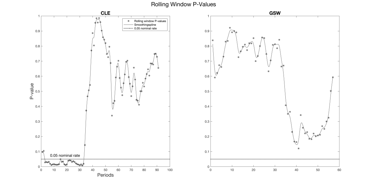
Figure 3: Rolling Window P-Values for the Best Lineups Over 2015-16 Season

However, interactions between players may vary over time and the test statistics aggregated for the entire season may mask the time-varying interaction effects. Therefore, we also examine the changes in the test statistic over the season using a rolling window analysis, where we repeatedly compute the p-value of the AR test statistic with a rolling window of fifty time periods. Figure 3 plots the p-values for the best lineups over the season.

[=== Figure 3 here ===]

In the case of GSW, p-values are still not small enough to reject the null. However, in the case of CLE, its p-value falls significantly below 0.05 between the 5th and 30th time periods, indicating that the player performances in the lineup were significantly interdependent during that time period. Overall, we observe substantial heterogeneity in the test statistics for the two lineups over the season, which strongly suggests that player interactions are not fixed, but change over time to adapt to the game environment.

6 Conclusion

This paper proposes an AR test for the statistical significance of dyad-specific peer effects in a linear panel data model of social interactions. The main advantage of the proposed test is that it does not require the specification of interaction structure. In our test, both the number of tested restrictions and the number of required IVs increase with the sample size, linking the literature on network models with unknown interaction structure and the literature on inference with many restrictions/IVs.

An important assumption of the proposed test is that the network effects are invariant over time. When the true network effects are time-varying, the proposed AR test may give misleading results. A partial solution to this problem is to conduct a rolling window analysis as illustrated in Section 5.2. Another restrictive assumption is that the random shocks $\epsilon_{it}$ need to be i.i.d. when individual and time fixed effects are present. The jackknife AR test statistic presented in Section 2 is robust to heteroskedasticity of unknown form, but the jackknife method is not appropriate in the presence of fixed effects. Although including fixed effects can alleviate the heteroskedasticity problem to a certain extent, developing a heteroskedasticity-robust test for network effects in the presence of fixed effects remains an important area for future research.

Appendix A Proofs

Proof of Proposition 1.

Under $H_{0}:\alpha=0$,

$$\frac{1}{\sqrt{K}}\widetilde{u}^{\prime}(P-D)\widetilde{u}$$

$$= \frac{1}{\sqrt{K}}[u-X(\widetilde{\beta}-\beta)]^{\prime}(P-D)[u-X(\widetilde{\beta}-\beta)]$$

$$= \frac{1}{\sqrt{K}}u^{\prime}(P-D)u+\frac{1}{\sqrt{K}}(\widetilde{\beta}-\beta)^{\prime}X^{\prime}(P-D)X(\widetilde{\beta}-\beta)$$

$$-\frac{1}{\sqrt{K}}(\widetilde{\beta}-\beta)^{\prime}X^{\prime}(P-D)u-\frac{1}{\sqrt{K}}u^{\prime}(P-D)X(\widetilde{\beta}-\beta).$$

As $PX=X$, it follows by Assumption 3 that

$$\frac{1}{\sqrt{K}}(\widetilde{\beta}-\beta)^{\prime}X^{\prime}(P-D)X(\widetilde{\beta}-\beta)=\frac{1}{\sqrt{K}}\sqrt{N}(\widetilde{\beta}-\beta)^{\prime}\frac{1}{N}(X^{\prime}X-X^{\prime}DX)\sqrt{N}(\widetilde{\beta}-\beta)=o_{p}(1).$$

Similarly,

$$\frac{1}{\sqrt{K}}(\widetilde{\beta}-\beta)^{\prime}X^{\prime}(P-D)u=\frac{1}{\sqrt{K}}\sqrt{N}(\widetilde{\beta}-\beta)^{\prime}\frac{1}{\sqrt{N}}(X^{\prime}u-X^{\prime}Du),$$

where $\mathrm{Var}(\frac{1}{\sqrt{N}}X^{\prime}u|X)=\frac{1}{N}X^{\prime}\Omega X$ and $\mathrm{Var}(\frac{1}{\sqrt{N}}X^{\prime}Du|X)=\frac{1}{N}X^{\prime}D\Omega DX$, and, hence, it follows by Assumption 3 and Markov’s inequality that

$$\frac{1}{\sqrt{K}}(\widetilde{\beta}-\beta)^{\prime}X^{\prime}(P-D)u=o_{p}(1).$$

Finally, as $\varsigma_{it}^{2}\geq\underline{\varsigma}^{2}>0$ and $P_{ii}\leq C_{p}<1$,

$$\Phi = \frac{2}{K}\mathrm{tr}[(P-D)\Omega(P-D)\Omega]\geq\frac{2\underline{\varsigma}^{4}}{K}\mathrm{tr}[(P-D)^{2}]=\frac{2\underline{\varsigma}^{4}}{K}\mathrm{tr}(P^{2}-DP-PD+D^{2})$$

$$= \frac{2\underline{\varsigma}^{4}}{K}[\mathrm{tr}(P)-\mathrm{tr}(D^{2})]\geq 2\underline{\varsigma}^{4}[1-\frac{C_{p}}{K}\mathrm{tr}(D)]=2\underline{\varsigma}^{4}(1-C_{p})>0.$$

Hence, it follows by Lemma A2 of Chao et al. (2012) that

$$\frac{1}{\sqrt{K}\sqrt{\Phi}}u^{\prime}(P-D)u\overset{d}{\rightarrow}N(0,1).$$

The desired result follows as $\widetilde{\Phi}-\Phi=o_{p}(1)$. ∎

Proof of Proposition 2.

Let $\lambda^{\ast}=K^{\ast}/N^{\ast}$. Under $H_{0}:\alpha=0$, as $P^{\ast}X^{\ast}=X^{\ast}$, $\epsilon^{\ast\prime}\epsilon^{\ast}=\epsilon^{\prime}J\epsilon$, and $\epsilon^{\ast\prime}P^{\ast}\epsilon^{\ast}=\epsilon^{\prime}P^{\ast}\epsilon$, we have

$$\frac{1}{\sqrt{K^{\ast}}}\widehat{\epsilon}^{\ast\prime}(P^{\ast}-\lambda^{\ast}I_{N})\widehat{\epsilon}^{\ast}$$

$$= \frac{1}{\sqrt{K^{\ast}}}[\epsilon^{\ast}-X^{\ast}(\widehat{\beta}-\beta)]^{\prime}(P^{\ast}-\lambda^{\ast}I_{N})[\epsilon^{\ast}-X^{\ast}(\widehat{\beta}-\beta)]$$

$$= \frac{1}{\sqrt{K^{\ast}}}\epsilon^{\prime}(P^{\ast}-\lambda^{\ast}J)\epsilon+\frac{1}{\sqrt{K^{\ast}}}(1-\lambda^{\ast})(\widehat{\beta}-\beta)^{\prime}X^{\ast\prime}X^{\ast}(\widehat{\beta}-\beta)$$

$$-\frac{1}{\sqrt{K^{\ast}}}(1-\lambda^{\ast})(\widehat{\beta}-\beta)^{\prime}X^{\ast\prime}\epsilon^{\ast}-\frac{1}{\sqrt{K^{\ast}}}(1-\lambda^{\ast})\epsilon^{\ast\prime}X^{\ast}(\widehat{\beta}-\beta)$$

$$= \frac{1}{\sqrt{K^{\ast}}}\epsilon^{\prime}(P^{\ast}-\lambda^{\ast}J)\epsilon+o_{p}(1),$$

where the last equality follows by Assumptions 1’-3’ and Markov’s inequality. As

$$J=(I_{T}-\frac{1}{T}\iota_{T}\iota_{T}^{\prime})\otimes(I_{n}-\frac{1}{n}\iota_{n}\iota_{n}^{\prime})=I_{N}-\frac{1}{T}(\iota_{T}\iota_{T}^{\prime})\otimes I_{n}-\frac{1}{n}I_{T}\otimes(\iota_{n}\iota_{n}^{\prime})+\frac{1}{N}(\iota_{T}\iota_{T}^{\prime})\otimes(\iota_{n}\iota_{n}^{\prime}),$$

where $N=nT$, we have

$$\frac{1}{\sqrt{K^{\ast}}}\epsilon^{\prime}(P^{\ast}-\lambda^{\ast}J)\epsilon$$

$$= \frac{1}{\sqrt{K^{\ast}}}\epsilon^{\prime}[P^{\ast}-\lambda^{\ast}I_{N}+\lambda^{\ast}\frac{1}{T}(\iota_{T}\iota_{T}^{\prime})\otimes I_{n}+\lambda^{\ast}\frac{1}{n}I_{T}\otimes(\iota_{n}\iota_{n}^{\prime})-\lambda^{\ast}\frac{1}{nT}(\iota_{T}\iota_{T}^{\prime})\otimes(\iota_{n}\iota_{n}^{\prime})]\epsilon$$

$$= \frac{1}{\sqrt{K^{\ast}}}\epsilon^{\prime}(P^{\ast}-\lambda I_{N})\epsilon+\frac{\lambda^{\ast}}{\sqrt{K^{\ast}}}\epsilon^{\prime}M\epsilon,$$

with $\lambda=K^{\ast}/N$ and

$$M=\frac{\lambda-\lambda^{\ast}}{\lambda^{\ast}}I_{N}+\frac{1}{T}(\iota_{T}\iota_{T}^{\prime})\otimes I_{n}+\frac{1}{n}I_{T}\otimes(\iota_{n}\iota_{n}^{\prime})-\frac{1}{nT}(\iota_{T}\iota_{T}^{\prime})\otimes(\iota_{n}\iota_{n}^{\prime}).$$

As $M$ is symmetric with a zero diagonal, $\mathrm{E}(\epsilon^{\prime}M\epsilon)=0$ and

$$\mathrm{Var}(\epsilon^{\prime}M\epsilon)=2\sigma^{4}\mathrm{tr}(M^{2})=2\sigma^{4}(n+T-\frac{n}{T}-\frac{T}{n}+\frac{2}{T}+\frac{2}{n}-\frac{1}{N}-3).$$

If $\lambda^{\ast}\rightarrow c$ for some $0<c<1$, then $K^{\ast}$ goes to infinity at the same rate as $N^{\ast}$, which implies $\mathrm{Var}(\frac{\lambda^{\ast}}{\sqrt{K^{\ast}}}\epsilon^{\prime}M\epsilon)=\frac{(\lambda^{\ast})^{2}}{K^{\ast}}\mathrm{Var}(\epsilon^{\prime}M\epsilon)=o(1)$. On the other hand, if $\lambda^{\ast}\rightarrow 0$, then $\mathrm{Var}(\frac{\lambda^{\ast}}{\sqrt{K^{\ast}}}\epsilon^{\prime}M\epsilon)=\frac{(\lambda^{\ast})^{2}}{K^{\ast}}\mathrm{Var}(\epsilon^{\prime}M\epsilon)=\frac{\lambda^{\ast}}{N^{\ast}}\mathrm{Var}(\epsilon^{\prime}M\epsilon)=o(1)$. Hence, for both cases, $\frac{\lambda^{\ast}}{\sqrt{K^{\ast}}}\epsilon^{\prime}M\epsilon=o_{p}(1)$ by Markov’s inequality, which implies

$$\frac{1}{\sqrt{K^{\ast}}}\epsilon^{\prime}(P^{\ast}-\lambda^{\ast}J)\epsilon=\frac{1}{\sqrt{K^{\ast}}}\epsilon^{\prime}(P^{\ast}-\lambda I_{N})\epsilon+o_{p}(1).$$

With a little abuse of the notation, let $\epsilon_{i}$ denote the $i$th element of $\epsilon$ and $P_{ij}^{\ast}$ denote the $(i,j)$th element of $P^{\ast}$. As $\sum_{i}(P_{ii}^{\ast}-\lambda)=0$,

$$\frac{1}{\sqrt{K^{\ast}}}\epsilon^{\prime}(P^{\ast}-\lambda I_{N})\epsilon$$

$$= \frac{1}{\sqrt{K^{\ast}}}\sum_{i}\sum_{j\neq i}P_{ij}^{\ast}\epsilon_{i}\epsilon_{j}+\frac{1}{\sqrt{K^{\ast}}}\sum_{i}(P_{ii}^{\ast}-\lambda)\epsilon_{i}^{2}-\frac{\sigma^{2}}{\sqrt{K^{\ast}}}\sum_{i}(P_{ii}^{\ast}-\lambda)$$

$$= \frac{1}{\sqrt{K^{\ast}}}\sum_{i}\sum_{j\neq i}P_{ij}^{\ast}\epsilon_{i}\epsilon_{j}+\sum_{i}\omega_{i},$$

where $\omega_{i}=(P_{ii}^{\ast}-\lambda)(\epsilon_{i}^{2}-\sigma^{2})/\sqrt{K^{\ast}}$. By construction, $\mathrm{E}(\omega_{i}|X_{i})=0$, where, with a little abuse of the notation, $X_{i}$ denotes the $i$th row of $X$. Under Assumptions 1’ and 2’, $\sum_{i}\mathrm{E}(\omega_{i}^{4})\rightarrow 0$ since $|P_{ii}^{\ast}-\lambda|<1$. Hence, it follows by Lemma A2 of Hansen et al. (2008) that

$$\frac{1}{\sqrt{K^{\ast}}\sqrt{\Phi^{\ast}}}\epsilon^{\prime}(P^{\ast}-\lambda I_{N})\epsilon\overset{d}{\rightarrow}N(0,1),$$

where

$$\Phi^{\ast}=\mathrm{E}[(\epsilon_{i}^{2}-\sigma^{2})^{2}]\mathrm{plim}_{N^{\ast}\rightarrow\infty}\frac{1}{K^{\ast}}\sum_{i}(P_{ii}^{\ast}-\lambda)^{2}+2\sigma^{4}[1-\mathrm{plim}_{N^{\ast}\rightarrow\infty}\frac{1}{K^{\ast}}\sum_{i}(P_{ii}^{\ast})^{2}].$$

Since $0\leq P_{ii}^{\ast}\leq 1$ and $\sum_{i}P_{ii}^{\ast}=K^{\ast}$, we have $\mathrm{plim}_{N^{\ast}\rightarrow\infty}\frac{1}{K^{\ast}}\sum_{i}(P_{ii}^{\ast})^{2}<1$, which implies $\Phi^{\ast}>0$. Rearranging terms, we can write $\Phi^{\ast}$ as

$$\Phi^{\ast}=(\mu_{4}-3\sigma^{4})[\mathrm{plim}_{N^{\ast}\rightarrow\infty}\frac{1}{K^{\ast}}\sum_{i}(P_{ii}^{\ast})^{2}-\bar{\lambda}]+2\sigma^{4}(1-\bar{\lambda}),$$

where $\bar{\lambda}=\lim_{N^{\ast}\rightarrow\infty}K^{\ast}/N$. The desired result follows as $\widehat{\Phi}^{\ast}-\Phi^{\ast}=o_{p}(1)$. ∎

Proof of Corollary 1.

Our proof follows the proof of Theorem 1 in Chao et al. (2014). Since $\sqrt{2K^{\ast}}AR_{FE}+K^{\ast}\geq q_{K^{\ast}-L}\left(1-\tau\right)$ if only if $AR_{FE}\geq\left(q_{K^{\ast}-L}\left(1-\tau\right)-K^{\ast}\right)/\sqrt{2K^{\ast}}$, the desired result follows from Proposition 2 and that

$$\frac{q_{K^{\ast}-L}\left(1-\tau\right)-K^{\ast}}{\sqrt{2K^{\ast}}}=\sqrt{\frac{K^{\ast}-L}{K^{\ast}}}\left(\frac{q_{K^{\ast}-L}\left(1-\tau\right)-\left(K^{\ast}-L\right)}{\sqrt{2\left(K^{\ast}-L\right)}}\right)-\frac{L}{\sqrt{2K^{\ast}}}\longrightarrow q(1-\tau),$$

where $q(1-\tau)$ is the $(1-\tau)$th quantile of the standard normal distribution and the convergence is due to the well-known property of chi-square distribution such that $\left(q_{f}(1-\tau)-r\right)/\sqrt{2f}$ $\longrightarrow q(1-\tau)$ as $f\to\infty$.∎

Appendix B Estimation of Excessive Kurtosis of Regression Error

We propose the following estimator for the excessive kurtosis of $\epsilon_{it}$, i.e., $\mu_{4}-3\sigma^{4}$:

$$\widehat{\kappa}=\widehat{\mu}_{4}-3\widehat{\sigma}^{4}\left(\frac{\pi_{1}}{\pi_{2}}\right),$$

where

$$\widehat{\mu}_{4}=\sum_{i=1}^{n}\sum_{t=1}^{T}\widehat{\epsilon}^{*4}_{it}/\pi_{2},\quad\widehat{\sigma}^{2}=\sum_{i=1}^{n}\sum_{t=1}^{T}\widehat{\epsilon}^{*2}_{it}/N^{*},\quad N^{*}=(n-1)(T-1),\quad N=nT,$$

$$\pi_{1}=\sum_{r=1}^{N}(J_{rr})^{2}=N^{*2}/N,\quad\pi_{2}=\sum_{r=1}^{N}\sum_{s=1}^{N}(J_{rs})^{4}=N^{*}(N^{*3}+(n-1)^{3}+(T-1)^{3}+1)/N^{3},$$

$$\text{$J_{rs}$ is the $(r,s)^{th}$ element of}\,\,J=(I_{T}-T^{-1}\iota_{T}\iota_{T}^{\prime})\otimes(I_{n}-n^{-1}\iota_{n}\iota_{n}^{\prime}),$$

$$\widehat{\epsilon}^{*}_{it}=\epsilon_{it}^{*}+X^{*}_{it}(\beta-\widehat{\beta}),\quad\epsilon_{it}^{*}=\epsilon_{it}-\bar{\epsilon}_{i.}-\bar{\epsilon}_{.t}+\bar{\epsilon}_{..},\,\,\bar{\epsilon}_{i.}=\sum_{t=1}^{T}\epsilon_{it}/T,\,\,\bar{\epsilon}_{.t}=\sum_{i=1}^{n}\epsilon_{it}/n,$$

$$\bar{\epsilon}_{..}=\sum_{i=1}^{n}\sum_{t=1}^{T}\epsilon_{it}/N,\,\text{and $X^{*}_{it}$ is similarly defined.}$$

All asymptotic results in this section hold for $T\to\infty$ and/or $n\to\infty$. We assume the following conditions for $X_{it}$:

Assumption B.1.

$X_{it}$ are i.i.d. over $i$ and $t$, and has finite moments up to order 8.

The i.i.d. assumption is to simplify the proof, and it can be relaxed with more lengthy arguments. See Stock & Watson (2008) for an example.

Proposition B.1.

Suppose Assumptions 1’ (in the main text) and B.1 hold. Under $H_{0}:\alpha=0$, $\widehat{\kappa}=\mu_{4}-3\sigma^{4}+o_{p}(1)$.

Proof of Proposition B.1..

To simply the calculations and notations, we consider the simple case with scalar $X_{it}$, and convert the two-dimensional index $(i,t)=(1,1)...,(n,T)$ to a one-dimensional index $i=1,...,N(=nT)$, while keeping the original ordering. Throughout the proof, we assume $n\geq 2$ and $T\geq 2$, and use the following properties of $J$ and Lemmas:

1. For all $i,j$ and $q\geq 1$, $J_{ii}=N^{*}/N$, $|J_{ij}|<1$, and $\sum_{j=1}^{N}J_{ij}=0$.

2. Since $J$ is symmetric & idempotent, $\sum_{r=1}^{N}J_{ir}J_{jr}=J_{ij}$, which implies $\sum_{r=1}^{N}J_{ir}^{2}=J_{ii}$.

Lemma B.1.

The elements of $J$ satisfy the following:

1. For $q\geq 1$, $0\leq\sum_{j=1}^{N}J_{ij}^{q}\leq\sum_{j=1}^{N}J_{ij}^{2}=N^{*}/N$, and $\sum_{j=1}^{N}|J_{ij}|^{q}\leq\sum_{j=1}^{N}|J_{ij}|=4N^{*}/N$

2. For $q_{1}\geq 1,q_{2}\geq 1$, $|\sum_{r=1}^{N}J_{ir}^{q_{1}}J_{jr}^{q_{2}}|\leq|J_{ij}|$.

Lemma B.2.

Suppose Assumption 1’ (in the main text) holds. Then, $\mathrm{E}\left[\left(\sum_{i=1}^{N}\epsilon_{i}^{*4}/\pi_{2}\right)^{2}\right]=\left(\mu_{4}-3\sigma^{4}+3\sigma^{4}\pi_{1}/\pi_{2}\right)^{2}+o(1).$

The proofs of the Lemmas are in the supplementary material.

To prove the consistency of $\widehat{\kappa}$, we first show $\widehat{\kappa}=\widetilde{\kappa}+o_{p}(1),$ where $\widetilde{\kappa}$ is defined as $\widehat{\kappa}$ with $\widehat{\epsilon}^{*}_{i}$ replaced by $\epsilon_{i}^{*}$. The statistics $\widetilde{\mu}$ and $\widetilde{\sigma}^{4}$ are similarly defined. First note that

$$\widehat{\mu}_{4} = \frac{N}{\pi_{2}}\sum_{i=1}^{N}\widehat{\epsilon}^{*4}_{i}/N$$

$$= \frac{N}{\pi_{2}}\left[\sum_{i=1}^{N}\epsilon_{i}^{*4}/N+4\left(\sum_{i=1}^{N}\epsilon_{i}^{*3}X_{i}^{*}/N\right)(\beta-\widehat{\beta})+6\left(\sum_{i=1}^{N}\epsilon_{i}^{*2}X_{i}^{*2}/N\right)(\beta-\widehat{\beta})^{2}\right.$$

$$\left.+4\left(\sum_{i=1}^{N}\epsilon_{i}^{*}X_{i}^{*3}/N\right)(\beta-\widehat{\beta})^{3}+\left(\sum_{i=1}^{N}X_{it}^{*4}/N\right)(\beta-\widehat{\beta})^{4}\right].$$

Since $\beta-\widehat{\beta}=O(1/\sqrt{N})$, it suffices to show that the four terms, $\sum_{i=1}^{N}\epsilon_{i}^{*3}X_{i}^{*}/N,$ $\sum_{i=1}^{N}\epsilon_{i}^{*2}X_{i}^{*2}/N,$ $\sum_{i=1}^{N}\epsilon_{i}^{*}X_{i}^{*3}/N$ and $\sum_{i=1}^{N}X_{it}^{*4}/N$ (hereafter, “the four terms”) are $O_{p}(1)$ to show $\widehat{\kappa}=\widetilde{\kappa}+o_{p}(1)$.

The transformed error $\epsilon^{*}_{i}$ is the $i^{th}$ element of $J\epsilon$, where $\epsilon$ is the error vector, so it can be written as $\epsilon^{*}_{i}=\sum_{j=1}^{N}J_{ij}\epsilon_{j}$. Then,

$$\mathrm{E}\left(\sum_{i=1}^{N}\epsilon_{i}^{*4}/N\right) = \sum_{i=1}^{N}\mathrm{E}\left(\sum_{j=1}^{N}\sum_{k=1}^{N}\sum_{l=1}^{N}\sum_{m=1}^{N}J_{ij}J_{ik}J_{il}J_{im}u_{j}u_{k}u_{l}u_{m}\right)/N$$ (11)

$$= \mu_{4}\sum_{i=1}^{N}\sum_{j=1}^{N}J_{ij}^{4}/N+3\sigma^{4}\sum_{i=1}^{N}\sum_{j=1}^{N}\sum_{k\neq j}J_{ij}^{2}J_{ik}^{2}/N$$

$$= (\mu_{4}-3\sigma^{4})\pi_{2}/N+3\sigma^{4}\sum_{i=1}^{N}\sum_{j=1}^{N}\sum_{k=1}^{N}J_{ij}^{2}J_{ik}^{2}/N$$

$$= (\mu_{4}-3\sigma^{4})\pi_{2}/N+3\sigma^{4}\pi_{1}/N,$$

which is bounded since $\epsilon_{it}$ has finite moments up to order 8, and $\pi_{1}/N=O(1)$ and $\pi_{2}/N=O(1)$. The second and last equalities are due to that $\epsilon_{it}$ are $i.i.d.$ and P2.

Note that the result (11) implies $\mathrm{E}(\epsilon_{i}^{*4})$ is finite and constant over $i$. Also, it can be easily seen from the proof of Lemma B.2 that $\mathrm{E}(\epsilon_{i}^{*8})$ is finite and constant over $i$. Similarly, it can be shown that both $\epsilon_{i}^{*}$ and $X_{i}^{*}$ have finite moments up to order 8, which implies that the expectations of the four terms are bounded. For example, $\mathrm{E}\left(\sum_{i=1}^{N}\epsilon_{i}^{*3}X_{i}^{*}/N\right)=\sum_{i=1}^{N}\mathrm{E}(\epsilon_{i}^{*3}X_{i}^{*})/N$, which is bounded since $|\mathrm{E}(\epsilon_{i}^{*3}X_{i}^{*})|\leq\mathrm{E}(|\epsilon_{i}^{*3}X_{i}^{*}|)\leq\sqrt{\mathrm{E}(\epsilon_{i}^{*6})\mathrm{E}(X_{i}^{*2})}$ by the Holder inequality. The same argument can be applied to the other terms.

Also, the variances of the four terms are bounded. For example, $\mathrm{Var}\left(\sum_{i=1}^{N}\epsilon_{i}^{*3}X_{i}^{*}/N\right)\leq(\sum_{i=1}^{N}\sqrt{\mathrm{Var}\left(\epsilon_{i}^{*3}X_{i}^{*}\right)}/N)^{2}$ by the covariance inequality, which is bounded since $\mathrm{Var}(\epsilon_{i}^{*3}X_{i}^{*})\leq\mathrm{E}(\epsilon_{i}^{*6}X_{i}^{*2})\leq\mathrm{E}(\epsilon_{i}^{*8})^{6/8}\mathrm{E}(X_{i}^{*8})^{1/4}$ by the Holder inequality.

Then, it follows that $\widehat{\mu}=\widetilde{\mu}+o_{p}(1)$, and the same result can be obtained for $\widehat{\sigma}^{4}$ by applying the same arguments, from which the desired result follows.

(B) Next, we show $\widetilde{\kappa}=\mu_{4}-3\sigma^{4}+o_{p}(1)$ by showing that (i) $\mathrm{E}(\widetilde{\kappa})=\mu_{4}-3\sigma^{4}+o(1)$ and (ii) $\mathrm{Var}(\widetilde{\kappa})=o(1)$.

(i) Similarly to (11),

$$\mathrm{E}\left[\left(\sum_{i=1}^{N}\epsilon_{i}^{*2}/N^{*}\right)^{2}\right] = \mathrm{E}\left[\left(\epsilon^{{}^{\prime}}J\epsilon\right)^{2}\right]/N^{*2}$$ (12)

$$= (\mu_{4}-3\sigma^{4})\pi_{1}/N^{*2}+\sigma^{4}(1+2/N^{*}).$$

Then, the results (11) and (12) yield

$$\mathrm{E}(\widetilde{\kappa}) = \frac{\mathrm{E}\left(\sum_{i=1}^{N}\epsilon_{i}^{*4}\right)}{\pi_{2}}-3\frac{\mathrm{E}\left[\left(\sum_{i=1}^{N}\epsilon_{i}^{*2}\right)^{2}\right]}{N^{*2}}\left(\frac{\pi_{1}}{\pi_{2}}\right)$$

$$= \mu_{4}-3\sigma^{4}-3\left(\frac{\pi_{1}}{\pi_{2}}\right)\left[(\mu_{4}-3\sigma^{4})\frac{\pi_{1}}{N^{*2}}+2\frac{\sigma^{4}}{N^{*}}\right]$$

$$= \mu_{4}-3\sigma^{4}+o(1),$$

where the last equality is due to $\pi_{1}/N^{*}=O(1)$ and $\pi_{1}/\pi_{2}=O(1)$.

(ii) Since $\mathrm{Var}(a+b)\leq(\sqrt{\mathrm{Var}(a)}+\sqrt{\mathrm{Var}(b)})^{2}$, it suffices to show $\mathrm{Var}(\widetilde{\mu})=o(1)$ and $\mathrm{Var}(\widetilde{\sigma}^{4})=o(1)$ to show $\mathrm{Var}(\widetilde{\kappa})=o(1)$. First, Lemma B.2 and result (11) yield that $\mathrm{Var}(\widetilde{\mu})=o(1)$. Also, the result (12) and that $\mathrm{E}(\widetilde{\sigma}^{2})=\sigma^{2}$ imply $\widetilde{\sigma}^{2}=\sigma^{2}+o_{p}(1)$. Then, by the Slutsky’s theorem, we have $\widetilde{\sigma}^{4}=\sigma^{4}+o_{p}(1)$, which implies $\mathrm{Var}(\widetilde{\sigma}^{4})=o(1)$. This completes the proof.

∎

Table 1: Empirical Size

			$\texttt{T}_{\texttt{DIN}}$		$\texttt{T}_{\texttt{AG}}$		$\texttt{T}_{\texttt{JL}}$
$n$	$T$	DGP	5%	1%	5%	1%	5%	1%
5	50	1	0.041	0.005	0.047	0.007	0.047	0.007
10	50	1	0.030	0.005	0.042	0.009	0.043	0.008
15	50	1	0.023	0.001	0.046	0.005	0.046	0.005
20	50	1	0.015	0.001	0.047	0.007	0.047	0.007
30	50	1	0.003	0.000	0.038	0.006	0.038	0.006
40	50	1	0.000	0.000	0.031	0.003	0.031	0.004
5	50	2	0.059	0.018	0.064	0.020	0.045	0.011
10	50	2	0.065	0.019	0.082	0.027	0.046	0.009
15	50	2	0.066	0.016	0.094	0.034	0.050	0.008
20	50	2	0.056	0.014	0.099	0.037	0.049	0.009
30	50	2	0.025	0.004	0.094	0.031	0.035	0.006
40	50	2	0.002	0.000	0.084	0.026	0.032	0.002

• Note: DGP1 and DGP2 use normal and log-normal errors, respectively. $\beta=1$. The estimator proposed in the Appendix is used to calculate the excessive kurtosis in $\texttt{T}_{\texttt{JL}}$. For all tests, chi-square distribution is used to calculate critical values.

Table 2: Summary Statistics

	Mean	Max	Median	Min	SD
$y$	65,644	180,156	63,363	13,510	25,320
$p$	0.009	0.033	0.007	-0.011	0.008
$s$	27.3	46.9	26.5	15.1	5.7

• Note: $y$ is the output-side real GDP per worker at chained PPPs (in mil. 2017US$), $p$ is the annual working-age population growth rate, and $s$ is the share of gross capital formation at current PPPs.

Table 3: AR Test for NBA Player Interactions

	CLE	GSW
Test statistic	44.20	24.39
P-value	0.23	0.96

Figure 1: Power Curves under Varying ND, $\rho$, and $\beta$ with Normal Errors

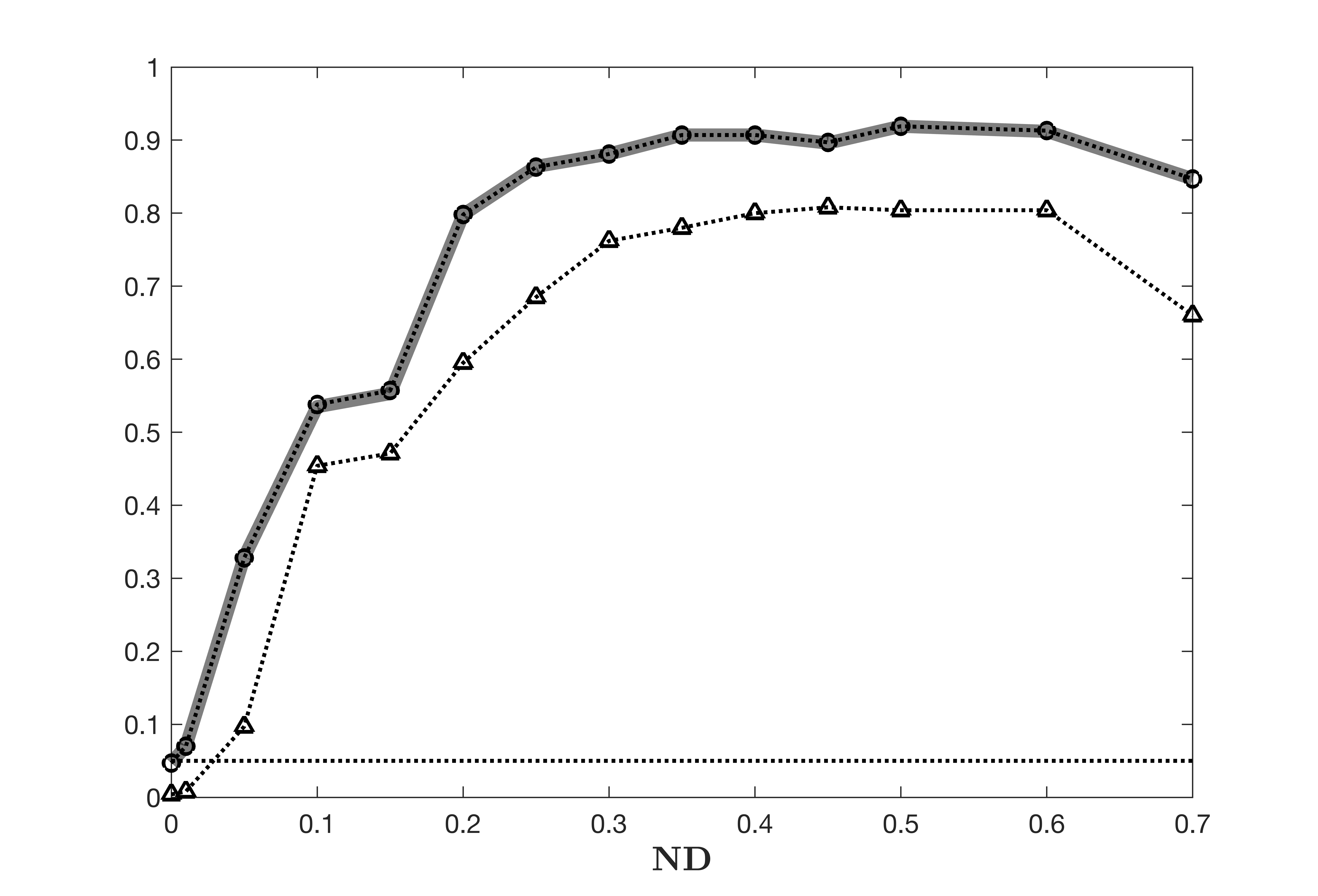
(a) $\rho$ = 0.3, $\beta=1$

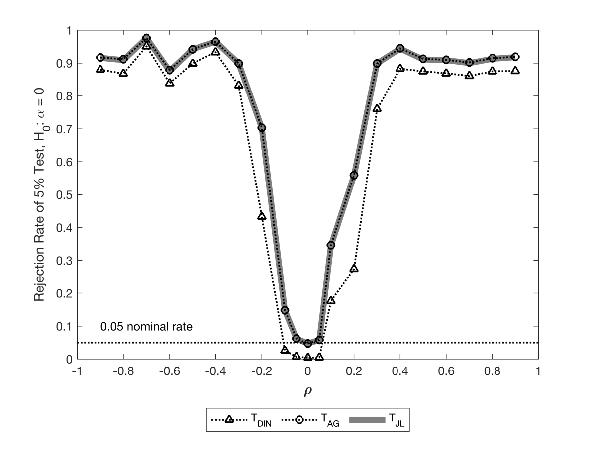
(b) ND = 0.3, $\beta=1$

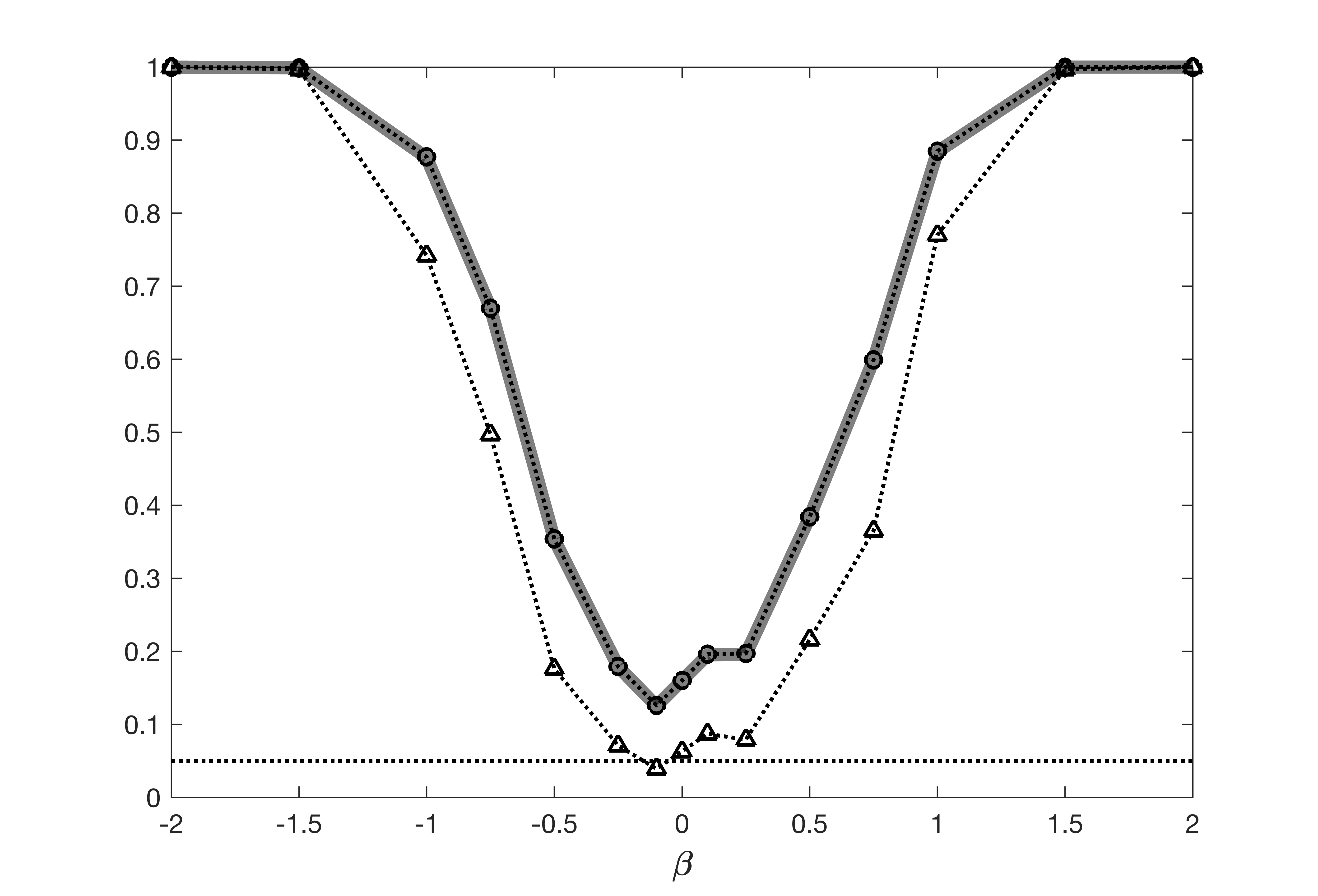
(c) $\rho$ = 0.3, $\texttt{ND}=0.3$

Figure 2: Power Curves under Varying ND, $\rho$, and $\beta$ with Log-Normal Errors

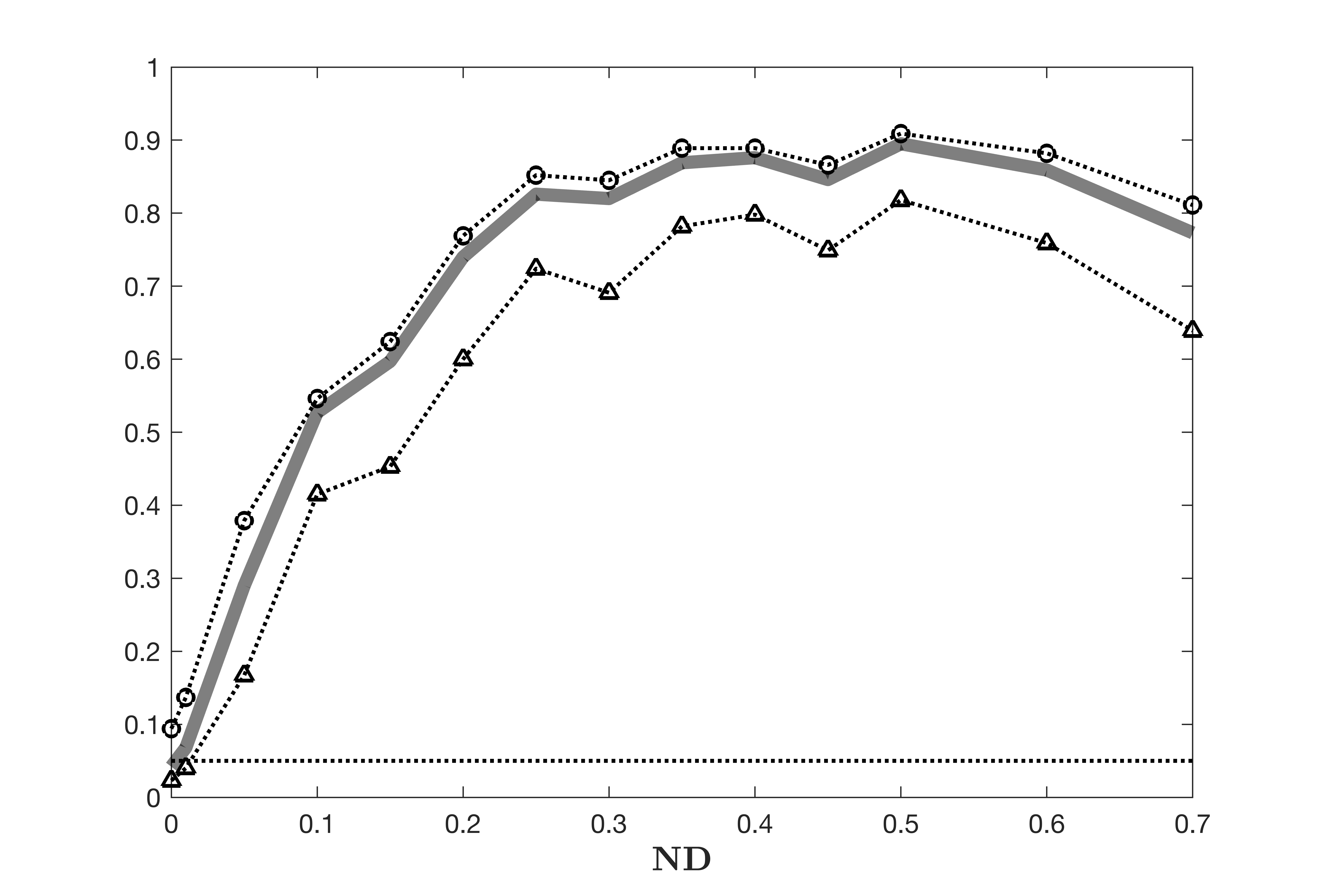
(a) $\rho$ = 0.3, $\beta=1$

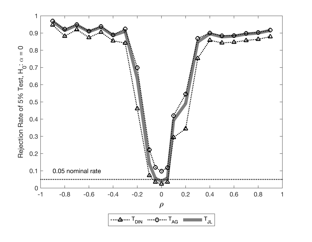
(b) ND = 0.3, $\beta=1$

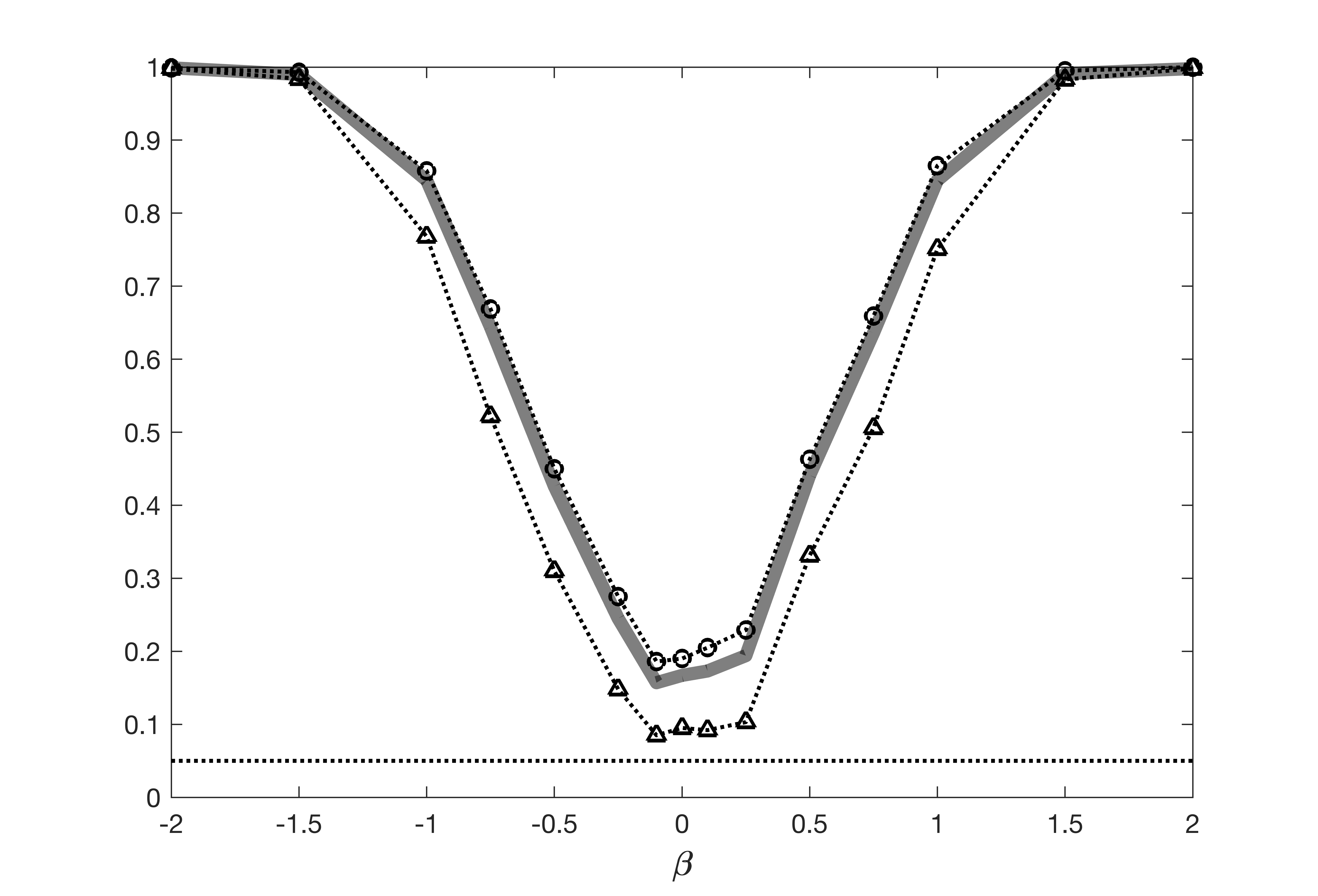
(c) $\rho$ = 0.3, $\texttt{ND}=0.3$

References

- (1)
- Anatolyev (2019) Anatolyev, S. (2019), ‘Many instruments and/or regressors: A friendly guide’, Journal of Economic Surveys 33(2), 689–726.
- Anatolyev & Gospodinov (2011) Anatolyev, S. & Gospodinov, N. (2011), ‘Specification testing in models with many instruments’, Econometric Theory 27(2), 427–441.
- Anatolyev & Solvsten (2023) Anatolyev, S. & Solvsten, M. (2023), Testing many restrictions under heteroskedasticity, forthcoming in Journal of Econometrics.
- Anatolyev & Yaskov (2017) Anatolyev, S. & Yaskov, P. (2017), ‘Asymptotics of diagonal elements of projection matrices under many instruments/regressors’, Econometric Theory 33(3), 717–738.
- Baltagi et al. (2012) Baltagi, B. H., Feng, Q. & Kao, C. (2012), ‘A lagrange multiplier test for cross-sectional dependence in a fixed effects panel data model’, Journal of Econometrics 170(1), 164–177.
- Battaglini et al. (2021) Battaglini, M., Patacchini, E. & Rainone, E. (2021), ‘Endogenous Social Interactions with Unobserved Networks’, The Review of Economic Studies 89(4), 1694–1747.
- Bekker (1994) Bekker, P. A. (1994), ‘Alternative approximations to the distributions of instrumental variable estimators’, Econometrica 62(3), 657–681.
- Berri (1999) Berri, D. j. (1999), ‘Who is most valuable? measuring the player’s production of wins in the nba’, Managerial and Decision Economics 20, 411–427.
- Blume et al. (2015) Blume, L. E., Brock, W. A., Durlauf, S. N. & Jayaraman, R. (2015), ‘Linear social interactions models’, Journal of Political Economy 123(2), 444–496.
- Bonaldi et al. (2015) Bonaldi, P., Hortaçsu, A. & Kastl, J. (2015), An empirical analysis of funding costs spillovers in the euro-zone with application to systemic risk, Working paper (http://www.nber.org/papers/w21462), National Bureau of Economic Research.
- Bramoullé et al. (2009) Bramoullé, Y., Djebbari, H. & Fortin, B. (2009), ‘Identification of peer effects through social networks’, Journal of Econometrics 150, 41–55.
- Chao et al. (2014) Chao, J. C., Hausman, J. A., Newey, W. K., Swanson, N. R. & Woutersen, T. (2014), ‘Testing overidentifying restrictions with many instruments and heteroskedasticity’, Journal of Econometrics 178, 15–21.
- Chao et al. (2012) Chao, J. C., Swanson, N. R., Hausman, J. A., Newey, W. K. & Woutersen, T. (2012), ‘Asymptotic distribution of jive in a heteroskedastic iv regression with many instruments’, Econometric Theory 28(1), 42–86.
- Chen et al. (2012) Chen, J., Gao, J. & Li, D. (2012), ‘A new diagnostic test for cross-section uncorrelatedness in nonparametric panel data models’, Econometric Theory 28(5), 1144–1163.
- Crudu et al. (2021) Crudu, F., Mellace, G. & Sándor, Z. (2021), ‘Inference in instrumental variable models with heteroskedasticity and many instruments’, Econometric Theory 37(2), 281–310.
- de Paula et al. (2020) de Paula, A., Rasul, I. & Souza, P. C. (2020), Identifying network ties from panel data: Theory and an application to tax competition. Working paper, University College London.
- Donald et al. (2003) Donald, S. G., Imbens, G. W. & Newey, W. K. (2003), ‘Empirical likelihood estimation and consistent tests with conditional moment restrictions’, Journal of Econometrics 117(1), 55–93.
- Ertur & Koch (2007) Ertur, C. & Koch, W. (2007), ‘Growth, technological interdependence and spatial externalities: theory and evidence’, Journal of Applied Econometrics 22(6), 1033–1062.
- Hansen et al. (2008) Hansen, C., Hausman, J. & Newey, W. (2008), ‘Estimation with many instrumental variables’, Journal of Business & Economic Statistics 26(4), 398–422.
- Ho et al. (2013) Ho, C.-Y., Wang, W. & Yu, J. (2013), ‘Growth spillover through trade: A spatial dynamic panel data approach’, Economics Letters 120(3), 450–453.
- Horrace et al. (2022) Horrace, W. C., Jung, H. & Sanders, S. (2022), ‘Network competition and team chemistry in the NBA’, Journal of Business and Economic Statistics 40(1), 35–49.
- Lee (2007) Lee, L. F. (2007), ‘Identification and estimation of econometric models with group interactions, contextual factors and fixed effects’, Journal of Econometrics 140, 333–374.
- Lewbel et al. (2023) Lewbel, A., Qu, X. & Tang, X. (2023), ‘Social networks with unobserved links’, Journal of Political Economy 131(4), 898–946.
- Liu & Prucha (2018) Liu, X. & Prucha, I. R. (2018), ‘A robust test for network generated dependence’, Journal of Econometrics 207(1), 92–113.
- Liu & Prucha (2023) Liu, X. & Prucha, I. R. (2023), On testing for spatial or social network dependence in panel data allowing for network variability, Working paper.
- Manresa (2016) Manresa, E. (2016), Estimating the structure of social interactions using panel data, Working paper.
- Manski (1993) Manski, C. F. (1993), ‘Identification of endogenous social effects: the reflection problem’, The Review of Economic Studies 60, 531–542.
- Mikusheva & Sun (2021) Mikusheva, A. & Sun, L. (2021), ‘Inference with Many Weak Instruments’, The Review of Economic Studies 89(5), 2663–2686.
- Moran (1950) Moran, P. A. P. (1950), ‘Notes on continuous stochastic phenomena’, Biometrika 37(1/2), 17–23.
- Ng (2006) Ng, S. (2006), ‘Testing cross-section correlation in panel data using spacings’, Journal of Business & Economic Statistics 24(1), 12–23.
- Pesaran (2021) Pesaran, M. H. (2021), ‘General diagnostic tests for cross-sectional dependence in panels’, Empirical Economics 60(1), 13–50.
- Pesaran et al. (2008) Pesaran, M. H., Ullah, A. & Yamagata, T. (2008), ‘A bias-adjusted lm test of error cross-section independence’, The Econometrics Journal 11(1), 105–127.
- Rose (2018) Rose, C. (2018), Identification of spillover effects using panel data, Working paper.
- Sarafidis et al. (2009) Sarafidis, V., Yamagata, T. & Robertson, D. (2009), ‘A test of cross section dependence for a linear dynamic panel model with regressors’, Journal of Econometrics 148(2), 149–161.
- Stock & Watson (2008) Stock, J. H. & Watson, M. W. (2008), ‘Heteroskedasticity-robust standard errors for fixed effects panel data regression’, Econometrica 76(1), 155–174.