Mimicking Better by Matching the Approximate Action Distribution

Abstract

In this paper, we introduce MAAD, a novel, sample-efficient on-policy algorithm for Imitation Learning from Observations. MAAD utilizes a surrogate reward signal, which can be derived from various sources such as adversarial games, trajectory matching objectives, or optimal transport criteria. To compensate for the non-availability of expert actions, we rely on an inverse dynamics model that infers plausible actions distribution given the expert’s state-state transitions; we regularize the imitator’s policy by aligning it to the inferred action distribution. MAAD leads to significantly improved sample efficiency and stability. We demonstrate its effectiveness in a number of MuJoCo environments, both int the OpenAI Gym and the DeepMind Control Suite. We show that it requires considerable fewer interactions to achieve expert performance, outperforming current state-of-the-art on-policy methods. Remarkably, MAAD often stands out as the sole method capable of attaining expert performance levels, underscoring its simplicity and efficacy.

1 Introduction

(a) DMC Suite

(b) OpenAI Gym

Figure 1: Median Normalized Return, over different environments, of various instantiations of our method (solid lines) versus baselines (dashed curves). Methods marked with ${\dagger}$ have access to expert actions representing the best possible performance, all others do not. More details on the construction of the figure in Section C.3.

Reinforcement learning (RL) trains agents to perform tasks by learning from rewards.Crafting a reward function that accurately reflects the intended task remains challenging (Silver et al., 2017; Ouyang et al., 2022). An alternative strategy involves teaching agents through demonstration, known as Imitation Learning (IL), where the goal is for the agent to closely replicate expert demonstrations, usually given as sequences of state-action pairs. While IL circumvents the complexity of designing reward functions, it requires access to expert actions, precluding its use in scenarios where actions are not observable, such as in motion capture data or video recordings.

Imitation learning from observations (ILO), as opposed to imitation learning from demonstrations (ILD), focuses on learning from states alone, allowing agents to imitate expert behavior without accessing their actions. This approach is more versatile, addressing the limitations of IL in many practical contexts, and has gained significant interest for its broader applicability in fields like autonomous driving. To facilitate imitation learning without direct action information, one strategy modifies algorithms to operate over state-state transitions rather than state-action pairs. This adaptation, as explored by (Torabi et al., 2019), leverages state-state transitions to distinguish between expert and agent. A different strand of research focuses on inferring missing actions through inverse models of the environment, facilitating the application of traditional IL methods (Hanna & Stone, 2017; Nair et al., 2017; Pavse et al., 2019; Al-Hafez et al., 2023).

Recent studies in ILD (Fujimoto & Gu, 2021; Jena et al., 2020; Yin et al., 2022; Haldar et al., 2022) have shown that integrating online IL techniques with offline Behavioral Cloning (BC) (Pomerleau, 1991; Bain & Sammut, 1995) improves sample efficiency by leveraging the strengths of both. Online IL methods learn through environmental interactions, whereas BC operates offline, making the interaction cost dependent solely on the online IL component. Another angle to improve sample efficiency is to adopt an online yet off-policy training strategy (Blondé & Kalousis, 2018; Kostrikov et al., 2020). In this context, (Zhu et al., 2021) propose combining an off-policy algorithm with a BC regularizer, employing an inverse model to address the absence of actions. However, off-policy approaches bring challenges such as extrapolation error and distributional shift (Fujimoto et al., 2018a; Fu et al., 2019; Levine et al., 2020). Instead, we propose an on-policy method for sample-efficient training in ILO that is both easy and stable to train.

Our approach combines a model-free base that dynamically infers rewards from environmental interactions, allowing for the use of different reward inference methods such as adversarial imitation, trajectory matching, and optimal transport, with a model-based regularizer that incorporates an inverse model of the environment. The inverse modeling task estimates the posterior distribution of actions that are plausible within the simulator’s physics, based on state transitions. The regularizer constrains the policy to align its actions closely with the action posterior distribution given by the inverse model as this is applied on expert demonstrations. This forms a secondary objective of action matching, which is similar to a BC objective.

We refer to our method as Mimicking Better by Matching the Approximate Action Distribution (MAAD). By guiding the policy towards selecting actions that comply with the physics intricately encoded within the simulator, we provide the agent with richer supervisory information throughout the training process. This results in significant sample efficiency gains; our policies train much faster than all competitive baselines, and they even train in settings where most of the other baselines fail. We demonstrate the superiority of our method on a spectrum of complex continuous control tasks developed with the MuJoCo physics engine (Todorov et al., 2012). We tackle the ones distributed in OpenAI Gym (Brockman et al., 2016) and in the DeepMind Control Suite (Tunyasuvunakool et al., 2020).

2 Related Work

Interest in Imitation Learning from Observations has grown in recent years, as it enables imitation from a variety of sources where actions are not explicit. Recent advancements have expanded the range of possibilities for reward approximation, such as adversarial methods, trajectory matching techniques, and optimal transport theory. In this work, we explore how to combine these with a behavior cloning-like regularizer that typically requires access to actions.

One strand of works for reward approximation adopts adversarial-based approaches and learn a discriminative function (discriminating between expert and agent data) that serves as a surrogate for the reward function. GAIL, (Ho & Ermon, 2016), is probably the most prominent example of adversarial-based methods for the ILD setting, relying on state-action pairs to discriminate between the expert and the agent. GAIfO, (Torabi et al., 2019), adapts GAIL to the ILO context by using state transitions instead of state-action pairs. Yang et al. (2019) have shown that GAIL and GAIfO are connected by the inverse dynamics disagreement; a divergence measure between the inverse dynamics models of the expert and the agent. Additionally, there have been efforts to adapt the GAIL framework to an off-policy setting, as seen in works by (Blondé & Kalousis, 2018) and (Kostrikov et al., 2018).

Another simple, but sometimes surprisingly effective, approach to reward approximation infers rewards based on trajectory matching distances; such works basically compute euclidean distances between the expert and agent sequences and use these as rewards (Englert et al., 2013; Peng et al., 2018). Finally, another approach to inferring surrogate rewards relies on Optimal Transport (OT). Optimal transport methods establish distribution alignments (joint distributions) that optimize some cost function when marginalized over the joint distribution. They are used in imitation learning to guide the agent’s distribution towards the expert’s distribution. For instance, SIL (Papagiannis & Li, 2020) uses Sinkhorn (Cuturi, 2013), PWIL (Dadashi et al., 2021) employs greedy Wasserstein, GDTW-IL is based on Gromov Dynamic Time Warping (Cohen et al., 2022), and GWIL (Fickinger et al., 2021) incorporates Gromov-Wasserstein (Peyré et al., 2016). Both trajectory matching and optimal transport approaches can also be easily deployed to the ILD or the ILO setting by operating over state-action, state-state or state-only sequences.

Adversarial- and optimal transport-based methods for imitation learning from demonstrations have been coupled with (regularized by) behavioral cloning, resulting in significant sample efficiency improvements compared to non-regularized baselines. GAIL-BC, (Jena et al., 2020), and ROT, (Haldar et al., 2022), regularize GAIL and SIL with behavioral cloning, respectively. Additional IL approaches that improve sample efficiency through BC include (Fujimoto & Gu, 2021; Yin et al., 2022). However, extending these sample efficiency gains to the ILO setting poses challenges due to the absence of actions.

Within the ILD setting a number of works take an alternative approach to address the non-availability of actions; instead of operating over state-state transitions they seek to infer the non-available actions. They do so by learning an inverse dynamics model, use it to infer the actions and continue with the application of standard ILD methods (Torabi et al., 2018; Hanna & Stone, 2017; Nair et al., 2017; Pavse et al., 2019; Al-Hafez et al., 2023). The availability of an inverse dynamics model that can account for the non-available actions opens the door for bringing the sample efficiency properties of behavioral cloning within the ILO context. (Zhu et al., 2021) follow such a path combining an off-policy imitation learning algorithm (Kostrikov et al., 2018) with a BC-like regularizer and demonstrate sample efficiency gains. Similarly, Hybrid-RL (Guo et al., 2019) merges standard RL with a BC-like regularizer; however, it assumes access to the expert’s reward function, which limits its broader applicability.

Our work brings the sample efficiency gains of behavioral-cloning regularization to on-policy imitation learning from observations by using inverse dynamics models to regularize the agent’s policy; we demonstrate its applicability with a diverse range of reward surrogate learning methods and show that it learns to imitate even in settings where competing methods simply fail.

3 Background

Markov Decision Process (MDP)

We will consider agents in a $\gamma$-discounted infinite horizon Markov decision process (MDP) $\mathcal{M}=\langle{\mathcal{S}},\mathcal{A},{\mathcal{T}},\rho_{0},r,\gamma\rangle$, where ${\mathcal{S}}$ and $\mathcal{A}$ are the state and action space respectively, ${\mathcal{T}}:{\mathcal{S}}\times\mathcal{A}\times{\mathcal{S}}\to\mathbb{R}_{\geq 0}$ is the transition distribution, $\rho_{0}:{\mathcal{S}}\to\mathbb{R}_{\geq 0}$ is the initial state distribution, $r:{\mathcal{S}}\times\mathcal{A}\rightarrow\mathbb{R}$ is the reward function and $\gamma$ is the discount factor.

Demonstrations and Observations

In the ILD setting, we have an expert $\pi_{e}$ which generates trajectories. A trajectory, $\tau$, is a sequence of state-action pairs, $\tau=\{(s_{0},a_{0}),(s_{1},a_{1}),\dots,(s_{T},a_{T})\}$, collected during one episode. We have access to a set of demonstrations $\mathcal{D}_{E}=\{\tau_{i}\},\tau_{i}\thicksim\pi_{e}$ on which we train our imitation policy. In contrast, in the ILO setting, we do not have access to actions. Here, a trajectory $\zeta$ is a sequence of state-state transitions, $\zeta=\{(s_{0},s_{1}),(s_{1},s_{2}),\dots,(s_{T-1},s_{T})\}$. As such, in this work, we train our imitation policy on the set of observations $\mathcal{D}_{E}=\{\zeta_{i}\},\zeta_{i}\thicksim\pi_{e}$.

Behavior Cloning

BC, (Pomerleau, 1991; Bain & Sammut, 1995), tackles imitation learning using supervised learning. The policy is trained to maximize the likelihood of the expert’s actions: $\mathcal{L}_{\mathrm{BC}}=-\mathbb{E}_{s,a\sim\mathcal{D}_{\text{E}}}[\log(\pi_{\theta}(a|s))]$. BC being basically a supervised learning method, it does not have an exploration mechanism. This makes the policy subject to compounding errors (Ross et al., 2010) and suboptimal asymptotic performance. BC also assumes the presence of expert state-action pairs in the demonstration set $\mathcal{D}_{\text{E}}$. To address the ILO setting in which we do not have actions, (Torabi et al., 2018) learn an inverse dynamics model, $p(a|s,s^{\prime})$, which they use to infer actions and they follow with a standard BC application. They train the inverse dynamics model on a dataset of $(s,a,s^{\prime})$ triplets collected with a random policy. Such an inverse model provides access to actions that are physically plausible with the given $(s,s^{\prime})$ transitions; these actions will typically be a superset of the actions that the expert would have chosen.

Occupancy Measure

The occupancy measure (OM) can be thought of as the distribution of states that are encountered in a Markov Decision Process (MDP) under a given policy $\pi$ (Ho & Ermon, 2016). The state OM, the most basic type of OM, is the discounted sum of the stationary state probability density, calculated over time for a given policy $\rho_{\pi}(s)=\sum_{t=0}^{\infty}\gamma^{t}P(s_{t}=s|\pi)$. We can use the state OM to define additional occupancy measures that are applicable to different supports within an MDP. These measures include the state-action occupancy measure $\rho_{\pi}(s,a)=\rho_{\pi}(s)\pi(a|s)$, the state-state transition occupancy measure $\rho_{\pi}(s,s^{\prime})=\int_{\mathcal{A}}\rho_{\pi}(s,\bar{a}){\mathcal{T}}(s^{\prime}|s,\bar{a}){\rm d}\bar{a}$, and the density function of the inverse dynamics model under the policy $\pi$, $\rho_{\pi}(a|s,s^{\prime})$ which is defined as follows:

$$\rho_{\pi}(a|s,s^{\prime}):=\frac{\mathcal{T}(s^{\prime}|s,a)\pi(a|s)}{\int_{\mathcal{A}}\mathcal{T}(s^{\prime}|s,\bar{a})\pi(\bar{a}|s)d\bar{a}}$$ (1)

where $\mathcal{T}(s^{\prime}|s,a)$ is the probability to transition to the next state $s^{\prime}$, given by the environment.

Generative Adversarial Imitation Learning

GAIL, (Ho & Ermon, 2016), minimizes the Jensen–Shannon divergence between the agent $\rho_{\pi}(s,a)$ and the expert $\rho_{\pi_{\text{E}}}(s,a)$ occupancy measures. The learned policy is thus given by $\operatorname*{\arg\min}_{\pi}\mathrm{D}_{\mathrm{JS}}(\rho_{\pi}(s,a)||\rho_{\pi_{\text{E}}}(s,a))$. In practice, this minimization is achieved by training a discriminator and a policy in an adversarial manner where the discriminator provides a proxy reward to an on-policy reinforcement learning algorithm, such as PPO (Schulman et al., 2017), that trains the policy. (Torabi et al., 2019) propose to replace the state-action occupancy measure with the state transition OM, thus the learned policy is given by $\operatorname*{\arg\min}_{\pi}\mathrm{D}_{\mathrm{JS}}(\rho_{\pi}(s,s^{\prime})||\rho_{\pi_{\text{E}}}(s,s^{\prime}))$, and thus eliminates the need for actions.

Trajectory Matching and Optimal Transport for Imitation Learning

Trajectory matching involves aligning the agent’s trajectory ($\xi^{\pi_{\theta}}_{i}$) with the expert’s trajectory ($\zeta^{E}_{i}$) to learn desired behaviors. This process typically employs a similarity measure to quantify how closely the agent’s states follow those of the expert. One common approach is using a cost function, such as Euclidean or cosine distance, to evaluate the difference at each point between $\xi^{\pi_{\theta}}_{i}$ and $\zeta^{E}_{i}$. The goal is to minimize this cost, guiding the agent towards replicating the expert’s trajectory as closely as possible. More recently, optimal transport (OT)-based techniques have been proposed in imitation learning (Dadashi et al., 2021; Papagiannis & Li, 2020; Cohen et al., 2022; Haldar et al., 2022). These methods focus on assessing the proximity between expert trajectories ($\zeta^{E}_{i}$) and agent trajectories ($\xi^{\pi_{\theta}}_{i}$) by evaluating the optimal transfer of probability mass from $\xi^{\pi_{\theta}}_{i}$ to $\zeta^{E}_{i}$. The surrogate reward for an observation is calculated as $r(s_{t})=-\sum_{t^{\prime}=1}^{T}C_{t,t^{\prime}}\mu^{*}_{t,t^{\prime}}$, where $C_{t,t^{\prime}}$ is a cost matrix $C_{t,t^{\prime}}=c(s_{t},s^{e}_{t^{\prime}})$, determining the cost of aligning a state from the agent’s trajectory $s$ with a state from the expert’s trajectory $s^{e}$. The term $\mu^{*}$ represents the optimal alignment between these trajectories.

4 Model

We will now introduce MAAD for Matching Approximate Action Distributions. As is typical in imitation learning, we aim to establish a policy $\pi_{\theta}$ that will closely mimic the expert’s policy $\pi_{e}$. In imitation learning from observations, this can be achieved by minimizing the discrepancy between the expert’s and agent’s state occupancy measures. This can be viewed as an alignment of the probability distributions over states that the expert and agent visit during their respective interactions with the environment. This corresponds to the following objective function:

$$\mathcal{L}_{\text{policy}}=\mathrm{D}(\rho_{\pi}(s,s^{\prime})||\rho_{\pi_{\text{E}}}(s,s^{\prime}))$$ (2)

In the context of imitation learning from demonstrations where the actions carried out by the expert are available, approaches such as (Fujimoto & Gu, 2021; Jena et al., 2020; Yin et al., 2022; Haldar et al., 2022) have shown that regularizing the imitator policy with a behavioral cloning objective significantly improves the convergence rate. Driven by this recurring result, we seek to also benefit from these advantages in the ILO setting by constraining our policy with such an auxiliary objective. Assuming for a moment that expert actions were available, we can define the following behavioral cloning loss term:

$$\mathcal{L}_{\text{BC}}=-\mathbb{E}_{s,a\sim\tau,\tau\sim\pi_{e}}[\log(\pi_{\theta}(a|s))]$$ (3)

which provides additional supervision to the learned policy by urging it to assign high probability to the actions that the expert selected in the demonstration dataset. We can thus extend the objective function in Eq. 2 with this loss term, resulting in the following regularized objective:

$$\mathcal{L}=\mathcal{L}_{\text{policy}}+\lambda\mathcal{L}_{\text{BC}}$$ (4)

The equation Eq. 4 is a generalization of existing BC-regularized IL algorithms. For instance, by substituting the state-state occupancy measure in Eq. 2 with a state-action occupancy measure, we obtain the GAIL-BC algorithm (Jena et al., 2020). On the other hand, if $\mathcal{L}_{\text{policy}}$ is based on TD3 (Fujimoto et al., 2018b), the resulting approach is TD3-BC (Fujimoto & Gu, 2021). Furthermore, if we introduce an OT-based trajectory matching approach for the state occupancy measure, we obtain the ROT algorithm (Haldar et al., 2022). As is obvious, this is applicable only to the ILD setting since the expectation in Eq. 3 is taken with respect to actions (and states) sampled from the expert.

If we are to use a loss term similar to the one in Eq. 3 to provide additional supervision, then we need a way to define what would be meaningful actions to select given that we do not have such information available from the expert data. The approach we take here is to learn the posterior distribution of actions that are physically plausible, under the used simulator, given a state-state transition, i.e. we want to approximate the true posterior $p(a|s,s^{\prime})$. What we have here is basically an instance of what is known as simulation-based inference (Cranmer et al., 2020), and in particular amortized posterior inference (Papamakarios & Murray, 2016; Lueckmann et al., 2017; Greenberg et al., 2019).

Learning the posterior distribution means actually solving the inverse dynamics problem of determining which are the actions that could have produced the observed $(s,s^{\prime})$ transition. We should stress here that these are not necessarily the actions that the expert would have chosen, they are rather a superset of the possible expert actions, since they are all plausible actions under the $(s,s^{\prime})$ transition. However, even though they are potentially a superset of the expert actions, they nevertheless provide considerable supervisory information since they will guide the expert to select actions that are physically plausible. Such guidance is particularly valuable since the gradients that we get from the Eq. 3 loss are much more informative than the ones that we get from the policy gradient optimization, since it is a supervised learning problem.

4.1 Inverse Dynamics Model (IDM)

Very often in inverse problems there is not a single inverse solution but rather a set of solutions and the respective posterior distribution has a multi-modal structure (Ardizzone et al., 2019). We thus choose to give the more general formulation to model the posterior distribution as a mixture density network (MDN) (Bishop, 1994) which by design models multi-modality; the learned posterior distribution is given by:

$$p_{\alpha,\psi}(a|s,s^{\prime})=\sum_{k=0}^{K-1}\alpha_{k}(s,s^{\prime})\psi_{k}(a|s,s^{\prime})$$ (5)

which is a mixture of $K$ distributions $\psi_{k}(a|s,s^{\prime})$ where $\alpha_{k}(s,s^{\prime})$ is the probability of picking the $k$-th component of the mixture for the state transition $(s,s^{\prime})$. We use Gaussians as the mixture components. The number of components $K$ is a hyperparameter, which depends on the environment. Despite having experimented with values of $K>1$ in preliminary sweeps, we found that for the considered suites of environments, $K=1$ was already yielding satisfactory results. This indicates that for both suites, leveraging the potential multimodality of inverse models was not instrumental, further strengthening the simplicity and robustness of the method.

To train the IDM model, we need to collect $(s,a,s^{\prime})$ triplets; a naive approach would be to collect such triplets using one or more random policies, but this would explore only a very small part of the joint space. Instead, we interleave the IDM training with the policy training. We take advantage of the interactions with the environment that take place as a result of learning online and push the collected triplets to a replay buffer $\mathcal{R}$. We train the inverse model $p_{\alpha,\psi}$ on the data from the replay buffer until convergence, update the policy and repeat the process. We warm-start the inverse model from the one obtained in the previous step. Note that the replay buffer will contain the $10^{5}$ most recent samples from different policies, starting from a random policy to the currently established policy. The inverse model is learned over all these data points. Even though these data points are obtained from different policies, the learned inverse model will be valid for all of them since it reflects the underlying physics implemented in the simulator, which are independent of the policy. We use the negative log-likelihood as the training objective for the inverse model:

$$\mathcal{L}_{\text{inv}}=-\mathbb{E}_{(s,a,s^{\prime})\sim\mathcal{R}}[\log(p_{\alpha,\psi}(a|s,s^{\prime}))]$$ (6)

4.2 Controlling the Policy Learning with the Inverse Dynamics Model

Our model has two basic components, a policy learning component which minimizes the loss given in Eq. 2 and an inverse model learning component which will be learned using the loss in Eq. 6. We will use the inverse model to further guide the policy learning with the help of a behavioral cloning loss similar to Eq. 3.

The policy learning component is basically an RL algorithm which minimizes Eq. 2 by learning the policy $\pi_{\theta}$ using Proximal Policy Optimization (PPO) (Schulman et al., 2017) where the surrogate rewards can come from different sources. In this paper, we will explore three different approaches for generating surrogate rewards. Firstly, we instantiate MAAD-AIL. This method obtains rewards through an adversarial training mechanism, similar to GAIfO (Torabi et al., 2019), where the agent’s goal is to mimic the expert’s behavior closely enough to fool a discriminator trained to distinguish between them. This implies training an additional model, namely the discriminator. We train the discriminator $D_{\phi}$ using the cross-entropy loss on $(s,s^{\prime})$ transitions sampled from the policy and the expert. The reward proxy that we use to train the policy is $r(s,s^{\prime})=-\log(1-D(s,s^{\prime}))$. Secondly, we explore the trajectory matching through MAAD-TM. In this approach, the agent’s and expert’s trajectories are considered to be aligned and of the same length, and the reward is calculated based on the Euclidean distance between the agent’s current state and the corresponding expert state at each step. This method is geared towards closely following the expert’s trajectory step by step. This method is naive and does not account for misalignment in the trajectories. It is therefore the fastest to compute because it relies on a simple distance that does not involve an extra model nor require an extra algorithm to be run. Lastly, we investigate an Optimal Transport (OT) based method, MAAD-OT. Here, rewards are obtained using the Sinkhorn algorithm (Cuturi, 2013), similar to what was proposed in SIL (Papagiannis & Li, 2020) and ROT (Haldar et al., 2022), with a cost matrix established on the cosine distance between states. This method is focused on minimizing the overall cost of transforming the agent’s state distribution to that of the expert, thereby assessing the similarity of entire trajectories. Note, the Sinkhorn algorithm needs to be run for each trajectory, and is expensive to run.

MAAD-AIL	MAAD-TM	MAAD-OT
$r(s_{t},s_{t+1})=$	$r(s_{t})=$	$r(s_{t})=$
$-\log(1-D(s_{t},s_{t+1}))$	$\|s_{t}-s_{t}^{e}\|$	$-\sum_{t^{\prime}=1}^{T}C_{t,t^{\prime}}\mu^{*}_{t,t^{\prime}}$

Table 1: Comparison of MAAD-AIL, MAAD-TM, and MAAD-OT reward formulations

The second component of our loss quantifies the similarity between the actions produced by the policy over expert states and the IDM predictions, using expert state-state transitions. The inverse model is represented by the learned posterior distribution $p_{\alpha,\psi}(a|s,s^{\prime})$. Given the policy and the inverse model, it becomes imperative to select a suitable behavioral cloning loss. An option to consider is a likelihood-based loss similar to that described in Equation 3. However, in this context, instead of sampling state-action pairs from the expert, we would sample $(s,s^{\prime})$ transitions. These transitions are then utilized to sample plausible actions from the learned inverse model, aiming to maximize the likelihood of these sampled actions under the policy.

$$-\mathbb{E}_{(s,s^{\prime})\sim\zeta,\zeta\sim\pi_{e}}\mathbb{E}_{a\sim p_{\alpha,\psi}(a|s,s^{\prime})}\log\pi_{\theta}(a|s)$$

Another alternative is to minimize the (forward) KL divergence of the inverse model and the learned policy, i.e.

$$\mathcal{L}_{\text{reg}}=\mathbb{E}_{(s,s^{\prime})\sim\zeta,\zeta\sim\pi_{e}}\mathrm{D}_{\mathrm{KL}}(p_{\alpha,\psi}(a|s,s^{\prime})||\pi_{\theta}(a|s))$$ (7)

the two approaches are equivalent up to an entropy term of the inverse model.

The forward KL induces a mode covering behavior. In our setting, this divergence will punish the policy for not assigning weight to actions that have non-zero density under the inverse model. Conversely, the reverse KL will punish the policy from having a non-zero density over actions for which the inverse model places none. In that respect, the mode-seeking effect induced by the reverse KL divergence should be the desired behavior, since it will push the learned policy to converge to one of the modes of the inverse model, and not fall in between the several potential modes discovered by the learned multi-modal inverse model. Considering our focus on sample efficiency, and given that preliminary experiments showed a $k=1$ to be sufficient, we chose to use the forward KL divergence to constrain the learned policy, similar to the approach in (Zhu et al., 2021). The forward KL divergence converges faster to the target distribution, i.e., the inverse model, thereby presenting a considerable advantage. Conversely, the reverse KL divergence necessitates extensive exploration to establish a reasonable policy, which is challenging during early training stages. Thus, the objective that we use to train the policy is:

$$\begin{split}\mathcal{L}=&\underbrace{\mathrm{D}(\rho_{\pi}(s,s^{\prime})||\rho_{\pi_{\text{E}}}(s,s^{\prime}))}_{\mathcal{L}_{\text{policy}}}\\ &+\underbrace{\mathbb{E}_{(s,s^{\prime})\sim\zeta,\zeta\sim\pi_{e}}\mathrm{D}_{\mathrm{KL}}(p_{\alpha,\psi}(a|s,s^{\prime})||\pi_{\theta}(a|s))}_{\mathcal{L}_{\text{reg}}}\end{split}$$ (8)

There are no gradients flowing back to the inverse model from the $\mathcal{L}_{\text{reg}}$ loss term. We give the complete training procedure in Algorithm 1.

Algorithm 1 Mimicking Better by Matching the Approximate Action Distribution (MAAD)

0:  Expert observations $\mathcal{D}_{E}=\{\zeta_{i}^{E}\}$ where $\zeta_{i}=\{(s_{0}^{E},s_{1}^{E}),(s_{1}^{E},s_{2}^{E}),...\}$, policy $\pi_{\theta}$, (discriminator $D_{\phi}$), inverse dynamics model $p_{\alpha,\psi}(a|s,s^{\prime})$, a replay buffer $\mathcal{R}$ and maximum number of iterations $M$

  Initialize replay buffer $\mathcal{R}$

  Initialize network parameters $\theta,(\phi),\alpha,\psi$

  for $1$ to $M$ do

     Collect agent rollouts $\mathcal{D}_{A}=\{\xi^{\pi_{\theta}}_{i}\}$, $\xi_{i}\thicksim\pi_{\theta}$, $\xi_{i}=\{(s_{0},a_{0},r_{0},s_{1}),(s_{1},a_{1},r_{1},s_{2}),...\}$, with $r_{i}$ from Table 1

     Add $\mathcal{D}_{A}$ to the replay buffer $\mathcal{R}$

     repeat

        Sample uniformly a minibatch $\mathcal{B}$ of state-action-state triplets from $\mathcal{R}$, $(s,a,s^{\prime})\sim\mathcal{R}$

        Update the inverse dynamics model $p_{\alpha,\psi}(a|s,s^{\prime})$

     until Inverse dynamics model $p_{\alpha,\psi}$ converges

     Update policy $\pi_{\theta}$ using $\mathcal{L}$ from Eq. 8

     (Update the discriminator $D_{\phi}$)

  end for

4.3 Discussion on Inverse Dynamics Disagreement

Yang et al. (2019) quantified the disparity between the learning objectives used within adversarial imitation learning from observations and demonstrations. They demonstrated that this disparity is quantified by the Inverse Dynamics Disagreement (IDD), which measures the disagreement between the inverse dynamics models of the expert and the learning agent.

$$\begin{split}&\underbrace{\mathrm{D}_{\mathrm{KL}}\left(\rho_{\pi}(a|s,s^{\prime})||\rho_{\pi_{\text{E}}}(a|s,s^{\prime})\right)}_{\text{IDD}}=\\ &\underbrace{\mathrm{D}_{\mathrm{KL}}\left(\rho_{\pi}(s,a)||\rho_{\pi_{\text{E}}}(s,a)\right)}_{\text{ILD}}-\underbrace{\mathrm{D}_{\mathrm{KL}}\left(\rho_{\pi}(s,s^{\prime})||\rho_{\pi_{\text{E}}}(s,s^{\prime})\right)}_{\text{ILO}}\end{split}$$ (9)

Thus, minimizing the ILD objective can be seen as jointly minimizing the learning objective of ILO and the IDD between the inverse dynamics models of the expert and the learning agent. Obviously, we have no way to access the inverse model of the expert, e.g. by learning a proxy of it, since we do not observe the expert’s actions.

Our regularizer, as defined in Eq. 7, minimizes the KL divergence between the inverse dynamics model of the environment, $\rho(a|s,s^{\prime})$, and the learned policy, $\pi_{\theta}(a|s)$, within the support of the state-state transitions observed from the expert. This KL divergence is an upper bound of the KL divergence between the IDMs of the environment and that of the agent, $\rho_{\pi}(a|s,s^{\prime})$, (refer to Appendix Section A.1 for the proof), i.e:

$$\begin{split}&\mathrm{D}_{\mathrm{KL}}\left(\rho(a|s,s^{\prime})||\rho_{\pi}(a|s,s^{\prime})\right)\leq\\ &\mathrm{D}_{\mathrm{KL}}\left(\rho(a|s,s^{\prime})||\pi_{\theta}(a|s)\right)+\text{Const}\end{split}$$ (10)

Thus, at optimality of Eq. 7, the inverse models of the environment and that of the learned agent align and we have $\rho(a|s,s^{\prime})=\rho_{\pi}(a|s,s^{\prime})$. This correspondence leads the IDD gap to be equal to the KL divergence between the environment’s and the expert’s inverse models:

$$\begin{split}&\mathrm{D}_{\mathrm{KL}}\left(\rho_{\pi}(a|s,s^{\prime})||\rho_{\pi_{\text{E}}}(a|s,s^{\prime})\right)=\\ &\mathrm{D}_{\mathrm{KL}}\left(\rho(a|s,s^{\prime})||\rho_{\pi_{\text{E}}}(a|s,s^{\prime})\right)\end{split}$$ (11)

We cannot manipulate any components on the right-hand side; the environment’s inverse model is governed by the simulator’s physics and the expert’s inverse model is dictated by the expert’s behavior, over which we have no control. The environment’s inverse model provides all conceivable actions that could lead to a given state-state transition under the simulator’s physics. Conversely, the expert’s inverse model is more selective, i.e. has smaller support, as it assigns non-zero probability only to actions the expert would have chosen for a specific state-state transition.

While ideally, we would want to minimize the IDD between the learned agent’s and the expert’s inverse models, the lack of access to the expert’s actions leaves us with no expert-specific choices. We chose to guide the agent towards actions that are physically plausible by deploying our regularizer. This guidance offers valuable supervision, compensating for the low-quality reward signal provided by the discriminator during early stages of adversarial training. Importantly, the training of the environment’s inverse model is a supervised process, which is considerably less complex and faster to converge than adversarial training.

5 Experiments

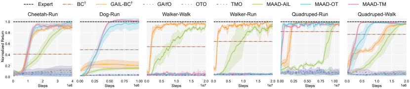
(a) DMC Suite

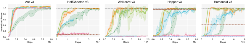
(b) OpenAI Gym

Figure 2: Performance comparison between our proposed version of MAAD and the baselines (some of the baselines, highlighted here with ${\dagger}$, have access to expert actions, Section 5.1 for more information). We average the results over three random seeds and show the mean and the range of one standard deviation.

To evaluate MAAD, we have conducted experiments on complex control tasks from the MuJoCo suite of environments (Todorov et al., 2012). We have used 6 locomotion tasks from DeepMind Control Suite and 5 from OpenAI Gym. The two suites differ on various aspects, such as their initial state distributions and termination criteria, posing their specific challenges to the learning algorithms, more details in Section B.1. We collected expert trajectories from a policy trained using PPO (Schulman et al., 2017) on each MuJoCo task. Then we used the collected trajectories to train several imitation learning baseline models and compare them against different flavors of our model. In the baseline models, we included not only ILO methods but also some ILD ones which have access to expert actions, these later ones should be seen as the best possible achievable performance if actions were observed. More details about environments, hyperparameters and training data and implementation can be found in Section B in appendix, and our code is openly available:

5.1 MAAD variants and Baselines

We evaluate three instantiations of MAAD, which differ on how surrogate rewards are obtained. We compare each one of them against its non-regularizer variant, where the KL regularizer is switched off. The first instantiation, MAAD-AIL, obtains surrogate rewards by adversarial imitation learning; we compare it against two variants of GAIL (Ho & Ermon, 2016): GAIfO (Torabi et al., 2019), which operates on observations and is essentially the non-regularized variant of MAAD-AIL, and GAIL-BC, which has access to expert actions. The second instantiation, MAAD-TM, obtains rewards relying on a trajectory matching approach; we employ the Euclidean distance metric for trajectory comparisons. We denote its non-regularized variant by TMO, for trajectory matching from observations. The third instantiation, MAAD-OT, is based on rewards sourced from optimal transport techniques. Specifically, it uses the Sinkhorn algorithm with a cosine distance-based cost matrix, akin to the frameworks of SIL and ROT. We denote its non-regularized variant by OTO, i.e. optimal transport from observations.

In addition to the non-regularized MAAD baselines, we also include a behavioral cloning baseline (BC) (Pomerleau, 1991; Bain & Sammut, 1995), which employs a supervised learning approach to learn the policy and requires action access. Although it is a fast training method since it does not require interactions with the environment, its asymptotic performance is suboptimal unless a substantial amount of expert data is available. We have also experimented with BCO (Torabi et al., 2018), the ILO variant of BC, which was consistently inferior to BC. Consequently, we decided not to include it in our reported results.

5.2 Results

We focus our comparative analysis of the different methods on sample efficiency, i.e. the number of environmental interactions required to achieve expert performance. We provide results for the DMC suite in Fig. 2(a) and for the OpenAI Gym in Fig. 2(b). The MAAD variants consistently surpassed their non-regularized counterparts, underscoring the importance of guidance and their aptitude in learning in the absence of expert actions. In the appendix Section C, we present detailed results, including a table summarizing the final performance and plots comparing the performance of the different models using either environment interactions or time.

The performance of the different MAAD variants varied based on evaluation suite, with some excelling in certain environments. In the DMC suite (Fig. 2(a)), the TM and OT variants of MAAD had very similar convergence rates, outperforming their non-regularized counterparts (TMO and OTO) as well as the MAAD-AIL variant, the latter in most but not all environments. Notably, the non-regularized variants, OTO and TMO, failed to converge within the allocated interaction budget, highlighting the critical role of guiding the policy even when using plausible actions as a substitute for actual expert actions. Among the AIL-based approaches, only GAIL-BC and MAAD-AIL achieved convergence to expert performance levels, GAIfO consistently underperformed. GAIL-BC systematically outperformed MAAD-AIL; however, it was comparable or slightly slower than MAAD-OT and MAAD-TM. It is noteworthy that in walker-based environments, specifically in run and walk tasks, only GAIL-BC and MAAD-AIL managed to converge to expert performance within the allotted budget. All TM- and OT-based methods struggled to learn in these environments. In Section D, we compare learned and expert actions, highlighting the challenges in walker-based environments.

In the OpenAI Gym suite (Fig. 2(b)), the scenario differs somewhat. While the non-regularized variants, OTO and TMO, follow a similar pattern to those in the DMC suite, i.e. they do not converge within the allocated number of interactions, now their regularized versions also face challenges in converging. For instance, MAAD-TM only converges in the Ant-v3 environment. MAAD-OT does achieve expert performance, but its rate of convergence is slower than that of the adversarial versions. In this suite, walker-based environments also appear to be particularly challenging for the OT and TM variants, as none of them managed to converge. Regarding the AIL variants, all three were capable of matching expert performance, with GAIL-BC and MAAD-AIL consistently outperforming GAIfO, demonstrating up to four times greater sample efficiency. A somewhat unexpected outcome was that MAAD-AIL also slightly outperformed GAIL-BC, given GAIL-BC’s access to expert actions. One possible explanation for that is that the inverse model on which MAAD relies to regularize the policy provides a broader range of, plausible, actions to choose from, offering more flexibility, compared to what happens in GAIL-BC where the regularizer guides the policy to exactly match the expert actions. Such a flexibility can be important in particular at the beginning of training, as matching expert actions precisely might be more challenging. Overall, MAAD-AIL is the method that achieves expert performance in both suites and all environments, except for the dog-run task in the DMC suite.

MAAD outperformed all the ILO baselines across various control tasks by exhibiting systematically faster convergence to expert performance, or in other terms, greater sample efficiency. Notably, for a good number of environments, a number of ILO-baselines did not even start converging. Its ability to learn effectively without expert actions makes it a powerful tool for tackling imitation learning from observations problems in real-world scenarios where expert states are hard and expensive to label accurately with action.

6 Conclusion

We presented Mimicking Better by Matching the Approximate Action Distribution (MAAD), a novel framework for imitation learning from observations.

The novelty of our approach lies in the integration of an inverse dynamics model in the on-policy imitation learning from observations setting. The inverse model provides access to the posterior distribution of physically plausible actions for a given state-state transition and serves as an auxiliary guide for the policy, providing the latter with meaningful action suggestions despite the absence of expert actions.

Our model combines the strengths of on-policy algorithms with behavioral cloning, effectively utilizing the benefits of both to speed-up learning. We integrate these components into a unified objective function that encourages the policy to mimic the expert’s state occupancy measure while also aligning with physically plausible actions as these are provided by the learned inverse model.

We empirically validated MAAD on a number of challenging tasks, demonstrating superior sample efficiency against all tested baselines. Notably, our method is able to achieve expert performance in settings in which some of the baselines do not even start training, and even matches the performance of baselines with access to expert actions.

Appendix A Proofs

A.1 Connecting Policy and Environment’s IDM through KL Divergence

In this section, we present the proof that our regularizer, as defined in Eq. 7, targets the minimization of the KL divergence between the inverse dynamics model of the environment, denoted as $\rho(a|s,s^{\prime})$, and the learned policy, $\pi_{\theta}$, over the support of the observed state-state transitions of the expert. More specifically, we show that this KL divergence is an upper bound on the divergence between the environment’s inverse dynamics model (IDM) and the agent’s IDM, represented as $\rho_{\pi}(a|s,s^{\prime})$. Therefore, we establish that:

$$\mathrm{D}_{\mathrm{KL}}\left(\rho(a|s,s^{\prime})||\rho_{\pi}(a|s,s^{\prime})\right)\leq\mathrm{D}_{\mathrm{KL}}\left(\rho(a|s,s^{\prime})||\pi_{\theta}(a|s)\right)+\text{Const}$$ (12)

Proof.

$$\mathrm{D}_{\mathrm{KL}}\left(\rho(a|s,s^{\prime})||\rho_{\pi}(a|s,s^{\prime})\right)$$

$$=\int_{{\mathcal{S}}\times\mathcal{A}\times{\mathcal{S}}}\rho(s,a,s^{\prime})\log\frac{\rho(a|s,s^{\prime})}{\rho_{\pi}(a|s,s^{\prime})}dsdads^{\prime}$$

$$=\int_{{\mathcal{S}}\times\mathcal{A}\times{\mathcal{S}}}\rho(s,a,s^{\prime})\log\frac{\rho(a|s,s^{\prime})}{\underbrace{\frac{\mathcal{T}(s^{\prime}|s,a)\pi_{\theta}}{\int_{\mathcal{A}}\mathcal{T}(s^{\prime}|s,\bar{a})\pi_{\theta}(\bar{a}|s)d\bar{a}}}_{\text{By def. Eq.~{}\ref{eq:inversemodel}}}}dsdads^{\prime}$$

$$=\int_{{\mathcal{S}}\times\mathcal{A}\times{\mathcal{S}}}\rho(s,a,s^{\prime})\log\frac{\rho(a|s,s^{\prime})\int_{\mathcal{A}}\mathcal{T}(s^{\prime}|s,\bar{a})\pi_{\theta}(\bar{a}|s)d\bar{a}}{\pi_{\theta}\mathcal{T}(s^{\prime}|s,a)}dsdads^{\prime}$$

$$=\int_{{\mathcal{S}}\times\mathcal{A}\times{\mathcal{S}}}\rho(s,a,s^{\prime})\log\frac{\rho(a|s,s^{\prime})}{\pi_{\theta}}dsdads^{\prime}+\int_{{\mathcal{S}}\times\mathcal{A}\times{\mathcal{S}}}\rho(s,a,s^{\prime})\log\frac{\int_{\mathcal{A}}\mathcal{T}(s^{\prime}|s,\bar{a})\pi_{\theta}(\bar{a}|s)d\bar{a}}{\mathcal{T}(s^{\prime}|s,a)}dsdads^{\prime}$$

$$\leq\mathrm{D}_{\mathrm{KL}}\left(\rho(a|s,s^{\prime})||\pi_{\theta}\right)+\sup_{\rho_{\pi}}\left(\int_{{\mathcal{S}}\times\mathcal{A}\times{\mathcal{S}}}\rho(s,a,s^{\prime})\log\frac{\int_{\mathcal{A}}\mathcal{T}(s^{\prime}|s,\bar{a})\pi_{\theta}(\bar{a}|s)d\bar{a}}{\mathcal{T}(s^{\prime}|s,a)}dsdads^{\prime}\right)$$

$$=\mathrm{D}_{\mathrm{KL}}\left(\rho(a|s,s^{\prime})||\pi_{\theta}\right)+\text{Const}$$

∎

The second term in the inequality, $\sup(.)$, is not subject to optimization with respect to the parameterized policy. Therefore, it can be regarded as a constant and we need only minimize the first term of the derived upper bound, i.e. $\mathrm{D}_{\mathrm{KL}}\left(\rho(a|s,s^{\prime})||\pi_{\theta}\right)$.

Appendix B Specifications

In this section, we give an account of the MuJoCo environments used in our experiments, the relevant aspects of our model’s implementation and the chosen hyperparameters.

B.1 Environments

We explored two suites, each with its own specificities. While OpenAI Gym employs a narrow initial state distribution, unnormalized rewards, and a termination signal when the agent falls, the DeepMind Control (dmc) suite utilizes a more challenging starting distribution, normalized rewards (i.e., each reward is in the range [0,1]), and a time limit termination of 1000 steps. Each of these suites presents distinct challenges to the learning process. OpenAI Gym’s simpler initial conditions and early termination policy tend to simplify training by limiting the exploration space. However, it employs non-normalized rewards, which may be more difficult to interpret. On the other hand, the DMC suite starts with a much larger initial state space and only terminates after the agent has performed 1000 timesteps in the environment. This significantly increases the complexity of exploration due to the greater number of possibilities. It utilizes normalized rewards, which tend to be easier for algorithms to learn from.

Table 2 provides a description of the state and action spaces of MuJoCo environments, along with the number and length of expert trajectories used to train our models. We use OpenAI Gym and the DMC suite as standard APIs to communicate with MuJoCo. For the OpenAI Gym environments, the versions associated with the name correspond to the version of the environment used in the Gym library.

It is important to note that AIL-based methods utilize only a subset of these trajectories. Following the approach in the original GAIL implementation (Ho & Ermon, 2016), we employ a subsampling rate of 20. This means that we retain only 50 state-action pairs (or state-state pairs, depending on whether the model requires actions or the next state) per trajectory. As a result, the number of expert samples used is effectively reduced from from $16000$ to $800$. In contrast, all other models utilize the full set of expert trajectories.

Environment	${\mathcal{S}}$	$\mathcal{A}$	Expert Trajectories
			$\#$ $\times$ Length
OpenAI Gym
Hopper-v3	$\mathbb{R}^{11}$	$\mathbb{R}^{3}$	16 $\times$ 1000
HalfCheetah-v3	$\mathbb{R}^{17}$	$\mathbb{R}^{6}$	16 $\times$ 1000
Walker2d-v3	$\mathbb{R}^{17}$	$\mathbb{R}^{6}$	16 $\times$ 1000
Ant-v3	$\mathbb{R}^{111}$	$\mathbb{R}^{8}$	16 $\times$ 1000
Humanoid-v3	$\mathbb{R}^{376}$	$\mathbb{R}^{17}$	16 $\times$ 1000
DMC Suite
Cheetah-Run	$\mathbb{R}^{17}$	$\mathbb{R}^{6}$	16 $\times$ 1000
Walker-Walk	$\mathbb{R}^{24}$	$\mathbb{R}^{6}$	16 $\times$ 1000
Walker-Run	$\mathbb{R}^{24}$	$\mathbb{R}^{6}$	16 $\times$ 1000
Quadruped-Run	$\mathbb{R}^{78}$	$\mathbb{R}^{12}$	16 $\times$ 1000
Quadruped-Walk	$\mathbb{R}^{78}$	$\mathbb{R}^{12}$	16 $\times$ 1000
Dog-Run	$\mathbb{R}^{223}$	$\mathbb{R}^{38}$	16 $\times$ 1000

Table 2: Description of MuJoCo environments and respective experts

B.2 Implementation Details

We implemented all the algorithms investigated and reported in PyTorch, maintaining a similar structure and keeping the same hyperparameters as much as possible. We used PPO (Schulman et al., 2017) as the underlying reinforcement learning algorithm.

All the online models, which require interactions with the environment, utilize 4 parallel workers for data collection and policy updates. These models share their computed gradients before optimization and receive the average gradients from all workers for policy updating. Moreover, we ran every experiment on the same set of 3 random seeds: ${0,1,2}$.

In imitation learning, access to expert trajectories is essential. We obtained these trajectories by training a policy using PPO (with the same architecture as the evaluated models) until convergence. At convergence, we generated 16 trajectories using this policy. These generated trajectories were saved and used to train all of our imitation learning models.

As noted in Section B.1, the adversarial imitation approaches use a subsample of the trajectories (50 samples per trajectory). This subsampling is achieved by randomly sampling state-action (or state-state) pairs from each expert trajectory. In contrast, all other methods, including Behavioral Cloning (BC), trajectory matching, and optimal transport-based approaches, have access to the entire expert trajectories.

For all the algorithms tested, the policy network consists of a two-layer MLP with 128 or 256 hidden units. The policy networks predicts only the mean of the action distribution as a function of the state, while the learned action variance is state-independent. The value and discriminator networks (when needed) adopt the same architecture as the policy. The inverse dynamics model also learns the variance independent of the state, which means it is set as parameters independent of the input.

Table 3 povide further details about the parameters used for the different algorithms.

B.3 Hyperparameters

Table 3 provides a comprehensive list of the hyperparameters used for each of the evaluated algorithms in Section 5.

	Parameter	Value
Shared	Batch size	64
	Rollout length	2048
	Discount $\gamma$	0.99
	$\pi$ architecture	{MLP [128,128], MLP [256,256]}
	$\pi$ Learning rate	$10^{-4}$
	$\pi$ updates	{3,6,9}
	GAIL $\lambda_{\text{entropy}}$	$0$
	PPO $\epsilon$	{0.1, 0.2}
	GAE $\lambda$	0.95
	Activation	$\tanh$
	Clip norm	0.5
	Gradient penalty	10
AIL-based	$\mathcal{D}$ architecture	MLP [128,128]
	$\mathcal{D}$ Learning rate	$10^{-4}$
	$\mathcal{D}$ updates	1
OT-based	Reward Scale Factor	20
	Sinkhorn # iterations	100
	Sinkhorn $\epsilon$	0.01
IDM	$\mathcal{R}$ size	$10^{5}$
	IDM architecture	MLP [128]
	IDM Learning Rate	$10^{-4}$
	IDM $K$	$1$
BC	Epochs	200
GAIL-BC${\dagger}$	$\lambda_{\text{reg}}$	{1, 10}
MAAD-*	$\lambda_{\text{reg}}$	{1, 10}

Table 3: Hyperparameters used for different algorithms, parameters in {} were submited to a sweep.

Appendix C Detailed Results

In Table 4 and Table 5, we detail the performance achieved with the learned policies. For each policy, we calculate the mean and the standard deviation across 50 generated trajectories. To facilitate visualization and comparison, we have highlighted all values that fall within 10% of the expert’s performance by rendering them in bold.

Model	Hopper-v3	HalfCheetah-v3	Walker2d-v3	Ant-v3	Humanoid-v3
Expert	3749 $\pm$ 31	11802 $\pm$ 172	7597 $\pm$ 64	6269 $\pm$ 132	7588 $\pm$ 34
GAIL-BC${\dagger}$	3832 $\pm$ 6	12038 $\pm$ 790	7993 $\pm$ 26	6612 $\pm$ 625	7821 $\pm$ 6
GAIfO	3842 $\pm$ 12	11403 $\pm$ 2136	7709 $\pm$ 660	6310 $\pm$ 1372	7776 $\pm$ 9
TMO	19 $\pm$ 0	-58 $\pm$ 85	1 $\pm$ 1	-185 $\pm$ 414	190 $\pm$ 54
OTO	41 $\pm$ 1	243 $\pm$ 223	22 $\pm$ 8	-337 $\pm$ 607	120 $\pm$ 37
MAAD-AIL	3822 $\pm$ 36	10506 $\pm$ 874	7537 $\pm$ 435	6655 $\pm$ 95	7557 $\pm$ 346
MAAD-TM	1544 $\pm$ 897	2331 $\pm$ 1089	360 $\pm$ 257	6205 $\pm$ 1448	480 $\pm$ 88
MAAD-OT	3713 $\pm$ 188	7552 $\pm$ 1154	211 $\pm$ 86	6333 $\pm$ 1142	7652 $\pm$ 321

Table 4: Learned policy performance for OpenAI Gym tasks. We report the mean and the standard deviation across 50 generated trajectories (some of the baselines, highlighted here with ${\dagger}$, have access to expert actions, Section 5.1 for more information).

Model	Cheetah-Run	Walker-Walk	Walker-Run	Quadruped-Run	Quadruped-Walk	Dog-Run
Expert	663 $\pm$ 121	932 $\pm$ 21	606 $\pm$ 34	748 $\pm$ 25	888 $\pm$ 63	382 $\pm$ 105
GAIL-BC${\dagger}$	692 $\pm$ 59	906 $\pm$ 139	592 $\pm$ 104	757 $\pm$ 34	885 $\pm$ 67	99 $\pm$ 60
GAIfO	91 $\pm$ 19	77 $\pm$ 24	37 $\pm$ 18	112 $\pm$ 159	100 $\pm$ 159	17 $\pm$ 4
TMO	98 $\pm$ 34	60 $\pm$ 31	38 $\pm$ 14	88 $\pm$ 157	125 $\pm$ 176	13 $\pm$ 3
OTO	62 $\pm$ 21	74 $\pm$ 29	36 $\pm$ 14	95 $\pm$ 116	97 $\pm$ 136	17 $\pm$ 5
MAAD-AIL	704 $\pm$ 39	823 $\pm$ 230	569 $\pm$ 154	745 $\pm$ 37	875 $\pm$ 72	99 $\pm$ 36
MAAD-TM	629 $\pm$ 179	133 $\pm$ 95	50 $\pm$ 20	755 $\pm$ 57	879 $\pm$ 73	408 $\pm$ 76
MAAD-OT	646 $\pm$ 145	63 $\pm$ 42	46 $\pm$ 23	744 $\pm$ 90	875 $\pm$ 76	398 $\pm$ 96

Table 5: Learned policy performance for DMC Suite tasks. We report the mean and the standard deviation across 50 generated trajectories (some of the baselines, highlighted here with ${\dagger}$, have access to expert actions, Section 5.1 for more information).

C.1 Interactions-based Comparison

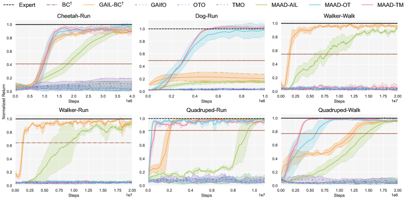
(a) DMC Suite

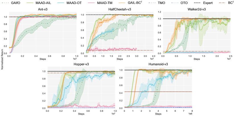
(b) OpenAI Gym

Figure 3: Interactions-based performance comparison of the different methods. Methods marked with ${\dagger}$, have access to expert actions, Section 5.1 for more information). We average the results over three random seeds and show the mean and the range of one standard deviation.

C.2 Time-based Comparison

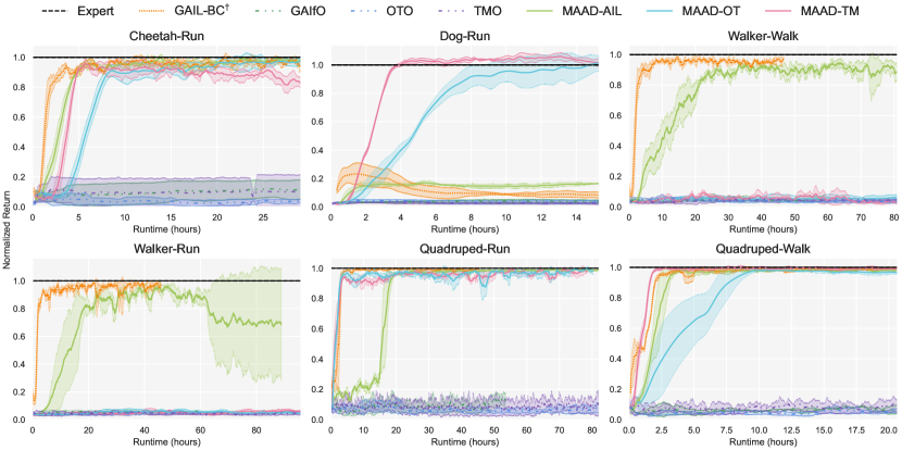
(a) DMC Suite

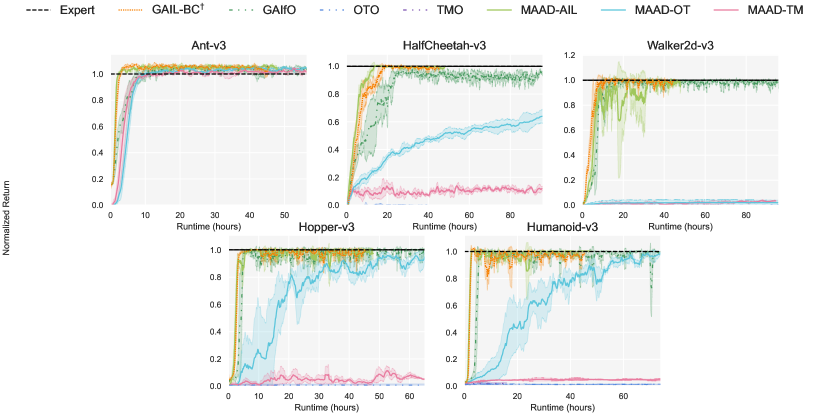
(b) OpenAI Gym

Figure 4: Computational time-based performance comparison of the different methods. Methods marked with ${\dagger}$, have access to expert actions, Section 5.1 for more information). We average the results over three random seeds and show the mean and the range of one standard deviation.

C.3 Median Normalized Return Comparison

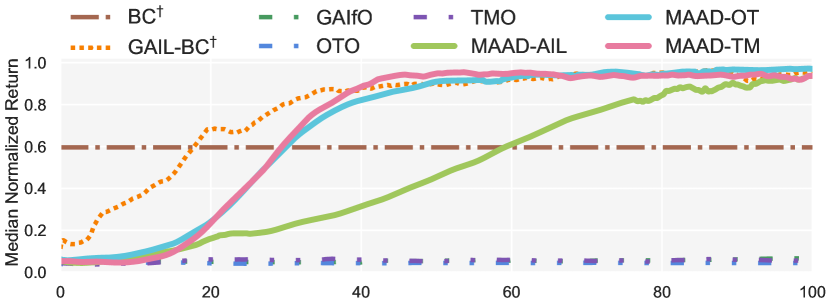
(a) DMC Suite

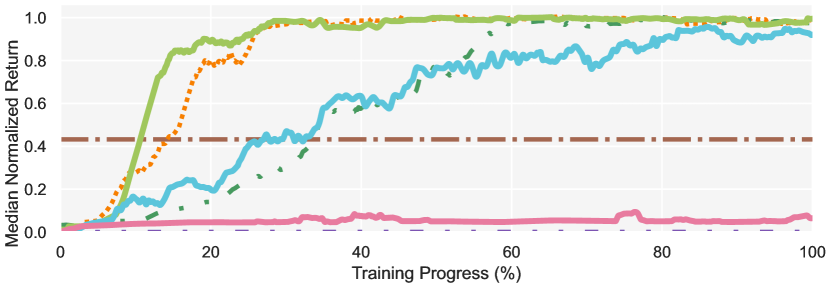
(b) OpenAI Gym

Figure 5: Median Normalized Return, over different environments, of various instantiations of our method (solid lines) versus baselines (dashed curves). This plot is derived by quantalising the training curves present in Fig. 3, using a fixed number of quantiles, here 5000, with median computation per algorithm across the different environments of each suite tested. Methods marked with ${\dagger}$ have access to expert actions representing the best possible performance, all others do not. More details on the construction of the figure in the appendix.

Appendix D Comparative Analysis of Learned and Expert Actions

Env	Algo	$\operatorname{R}^{2}(\pi_{\theta}(a|s^{E}),a^{E})$	$\operatorname{R}^{2}(\operatorname{IDM}(a|s^{E}_{t},s^{E}_{t+1}),a^{E})$
Ant-v3	MAAD-AIL	0.8998 $\pm$ 6.87e-03	0.9492 $\pm$ 7.20e-03
	MAAD-TM	0.9350 $\pm$ 4.76e-03	0.9621 $\pm$ 4.64e-03
	MAAD-OT	0.9255 $\pm$ 1.05e-02	0.9530 $\pm$ 9.89e-03
HalfCheetah-v3	MAAD-AIL	0.9952 $\pm$ 2.82e-04	0.9991 $\pm$ 1.78e-04
	MAAD-TM	0.8719 $\pm$ 5.23e-02	0.8762 $\pm$ 5.29e-02
	MAAD-OT	0.9916 $\pm$ 1.62e-03	0.9956 $\pm$ 1.65e-03
Walker2d-v3	MAAD-AIL	0.8297 $\pm$ 2.62e-02	0.8575 $\pm$ 2.62e-02
	MAAD-TM	0.0192 $\pm$ 2.34e-01	0.0238 $\pm$ 2.35e-01
	MAAD-OT	-0.5949 $\pm$ 3.30e-01	-0.5816 $\pm$ 3.31e-01
Hopper-v3	MAAD-AIL	0.7943 $\pm$ 1.13e-01	0.8072 $\pm$ 1.06e-01
	MAAD-TM	0.5033 $\pm$ 1.66e-01	0.5196 $\pm$ 1.64e-01
	MAAD-OT	0.9223 $\pm$ 2.53e-02	0.9269 $\pm$ 2.59e-02
Humanoid-v3	MAAD-AIL	0.9614 $\pm$ 3.01e-03	0.9956 $\pm$ 8.67e-05
	MAAD-TM	0.9233 $\pm$ 4.92e-03	0.9944 $\pm$ 1.07e-03
	MAAD-OT	0.9782 $\pm$ 2.04e-03	0.9958 $\pm$ 2.26e-05
Cheetah-Run	MAAD-AIL	0.9500 $\pm$ 4.00e-03	0.9920 $\pm$ 4.18e-03
	MAAD-TM	0.9809 $\pm$ 1.39e-03	0.9898 $\pm$ 1.44e-03
	MAAD-OT	0.9823 $\pm$ 4.26e-03	0.9913 $\pm$ 3.80e-03
Dog-Run	MAAD-AIL	0.9517 $\pm$ 1.32e-03	0.9966 $\pm$ 3.01e-03
	MAAD-TM	0.9700 $\pm$ 2.17e-04	0.9985 $\pm$ 1.61e-05
	MAAD-OT	0.9730 $\pm$ 1.12e-03	0.9984 $\pm$ 3.86e-05
Walker-Walk	MAAD-AIL	0.6387 $\pm$ 3.70e-03	0.7145 $\pm$ 1.13e-02
	MAAD-TM	-0.1460 $\pm$ 2.34e-01	-0.1461 $\pm$ 2.34e-01
	MAAD-OT	-0.1965 $\pm$ 2.96e-01	-0.1955 $\pm$ 3.12e-01
Walker-Run	MAAD-AIL	0.7835 $\pm$ 2.52e-02	0.8025 $\pm$ 2.44e-02
	MAAD-TM	-0.1207 $\pm$ 1.69e-01	-0.1209 $\pm$ 1.69e-01
	MAAD-OT	-0.1794 $\pm$ 1.93e-01	-0.1796 $\pm$ 1.92e-01
Quadruped-Run	MAAD-AIL	0.8200 $\pm$ 4.31e-04	0.9995 $\pm$ 8.24e-06
	MAAD-TM	0.8947 $\pm$ 2.82e-03	0.9978 $\pm$ 7.60e-04
	MAAD-OT	0.8901 $\pm$ 1.90e-03	0.9972 $\pm$ 4.89e-04
Quadruped-Walk	MAAD-AIL	0.9261 $\pm$ 2.94e-03	0.9994 $\pm$ 7.14e-05
	MAAD-TM	0.9787 $\pm$ 1.55e-03	0.9994 $\pm$ 2.38e-06
	MAAD-OT	0.9582 $\pm$ 5.39e-04	0.9994 $\pm$ 1.04e-05

Table 6: Comparison of R-squared Scores for Policy and Inverse Dynamics Model Against Expert Actions Across Different Environments and Algorithms

Even though we operate within the Imitation Learning from Observations (ILO) framework, where trained models do not have direct access to expert actions, we possess these actions since we trained the experts. We would like to understand better how the actions that MAAD trained policies select, as well as these that the inverse model selects, relate to the expert’s actions. As already discussed in Section 4.3, the inverse model learns the distribution of plausible actions, if this is done well, the expert’s action will have a distribution that has a support that is a subset of the support of the plausible actions’ distribution. To understand the relations described above, we computed the R-squared score between the actions produced by our learned policies and the true expert actions, as well as between the learned IDM and the expert actions. Values below an R-squared score of 0.5 were highlighted in red. The majority of our models achieved an R-squared score close to one, i.e. most often there is a high to very high agreement between the learning policy, the inverse model, and the expert’s choices. Again, we want to stress that one should not interpret that, in the general case, as the inverse model eventually learning the expert; we rather believe that for the majority of the environments that we consider here the set of plausible actions is rather constrained, after all we have seen that the unimodality assumption ($k=1$ for IDM Section 4.1) works best in most of the environments; thus the expert actions can only fall within this rather constrained unimodal set of plausible actions. Under such conditions, it is expected that the actions learned by both the policy and the inverse model would align closely with those of the expert.

A notable exception to this high agreement pattern are the walker-based environments, where we observed the poorest performance, in some cases resulting even in negative R-squared values. One possible explanation is that these environments are not strictly unimodal, leading to difficulties in action learning. This is something that we want to investigate further by focusing on more challenging environments which feature a less constrained set of plausible actions.

References

- Al-Hafez et al. (2023) Al-Hafez, F., Tateo, D., Arenz, O., Zhao, G., and Peters, J. Ls-iq: Implicit reward regularization for inverse reinforcement learning. arXiv preprint arXiv:2303.00599, 2023.
- Ardizzone et al. (2019) Ardizzone, L., Kruse, J., Wirkert, S. J., Rahner, D., Pellegrini, E., Klessen, R. S., Maier-Hein, L., Rother, C., and Köthe, U. Analyzing inverse problems with invertible neural networks. 2019.
- Bain & Sammut (1995) Bain, M. and Sammut, C. A framework for behavioural cloning. In Machine Intelligence 15, 1995.
- Bishop (1994) Bishop, C. M. Mixture density networks. 1994.
- Blondé & Kalousis (2018) Blondé, L. and Kalousis, A. Sample-efficient imitation learning via generative adversarial nets. In International Conference on Artificial Intelligence and Statistics, 2018.
- Brockman et al. (2016) Brockman, G., Cheung, V., Pettersson, L., Schneider, J., Schulman, J., Tang, J., and Zaremba, W. Openai gym. arXiv preprint arXiv:1606.01540, 2016.
- Cohen et al. (2022) Cohen, S., Amos, B., Deisenroth, M. P., Henaff, M., Vinitsky, E., and Yarats, D. Imitation learning from pixel observations for continuous control, 2022.
- Cranmer et al. (2020) Cranmer, K., Brehmer, J., and Louppe, G. The frontier of simulation-based inference. Proceedings of the National Academy of Sciences of the United States of America, 117(48):30055–30062, 2020. ISSN 10916490. doi: 10.1073/pnas.1912789117.
- Cuturi (2013) Cuturi, M. Sinkhorn distances: Lightspeed computation of optimal transport. In Burges, C., Bottou, L., Welling, M., Ghahramani, Z., and Weinberger, K. (eds.), Advances in Neural Information Processing Systems, volume 26. Curran Associates, Inc., 2013. URL https://proceedings.neurips.cc/paper_files/paper/2013/file/af21d0c97db2e27e13572cbf59eb343d-Paper.pdf.
- Dadashi et al. (2021) Dadashi, R., Hussenot, L., Geist, M., and Pietquin, O. Primal wasserstein imitation learning. ICLR, 2021.
- Englert et al. (2013) Englert, P., Paraschos, A., Peters, J., and Deisenroth, M. P. Model-based imitation learning by probabilistic trajectory matching. 2013 IEEE International Conference on Robotics and Automation, pp. 1922–1927, 2013.
- Fickinger et al. (2021) Fickinger, A., Cohen, S., Russell, S. J., and Amos, B. Cross-domain imitation learning via optimal transport. ArXiv, abs/2110.03684, 2021.
- Fu et al. (2019) Fu, J., Kumar, A., Soh, M., and Levine, S. Diagnosing bottlenecks in deep q-learning algorithms. In International Conference on Machine Learning, 2019.
- Fujimoto & Gu (2021) Fujimoto, S. and Gu, S. S. A minimalist approach to offline reinforcement learning. In Advances in Neural Information Processing Systems (NeurIPS), 2021.
- Fujimoto et al. (2018a) Fujimoto, S., Meger, D., and Precup, D. Off-policy deep reinforcement learning without exploration. In International Conference on Machine Learning, 2018a.
- Fujimoto et al. (2018b) Fujimoto, S., van Hoof, H., and Meger, D. Addressing function approximation error in actor-critic methods. In International Conference on Machine Learning, 2018b.
- Greenberg et al. (2019) Greenberg, D., Nonnenmacher, M., and Macke, J. Automatic posterior transformation for likelihood-free inference. In International Conference on Machine Learning, pp. 2404–2414. PMLR, 2019.
- Guo et al. (2019) Guo, X., Chang, S., Yu, M., Tesauro, G., and Campbell, M. Hybrid reinforcement learning with expert state sequences. In AAAI Conference on Artificial Intelligence, 2019.
- Haldar et al. (2022) Haldar, S., Mathur, V., Yarats, D., and Pinto, L. Watch and match: Supercharging imitation with regularized optimal transport. In Conference on Robot Learning, 2022.
- Hanna & Stone (2017) Hanna, J. P. and Stone, P. Stochastic grounded action transformation for robot learning in simulation. 2020 IEEE/RSJ International Conference on Intelligent Robots and Systems (IROS), pp. 6106–6111, 2017.
- Ho & Ermon (2016) Ho, J. and Ermon, S. Generative adversarial imitation learning. In Advances in Neural Information Processing Systems (NeurIPS), 2016.
- Jena et al. (2020) Jena, R., Liu, C., and Sycara, K. P. Augmenting gail with bc for sample efficient imitation learning. In Conference on Robot Learning, 2020.
- Kostrikov et al. (2018) Kostrikov, I., Agrawal, K. K., Dwibedi, D., Levine, S., and Tompson, J. Discriminator-actor-critic: Addressing sample inefficiency and reward bias in adversarial imitation learning. ArXiv, abs/1809.02925, 2018.
- Kostrikov et al. (2020) Kostrikov, I., Nachum, O., and Tompson, J. Imitation learning via off-policy distribution matching. In International Conference on Learning Representations, ICLR, 2020.
- Levine et al. (2020) Levine, S., Kumar, A., Tucker, G., and Fu, J. Offline reinforcement learning: Tutorial, review, and perspectives on open problems. ArXiv, abs/2005.01643, 2020.
- Lueckmann et al. (2017) Lueckmann, J.-M., Gonçalves, P. J., Bassetto, G., Öcal, K., Nonnenmacher, M., and Macke, J. H. Flexible statistical inference for mechanistic models of neural dynamics. In Proceedings of the 31st International Conference on Neural Information Processing Systems, pp. 1289–1299, 2017.
- Nair et al. (2017) Nair, A., Chen, D., Agrawal, P., Isola, P., Abbeel, P., Malik, J., and Levine, S. Combining self-supervised learning and imitation for vision-based rope manipulation. 2017 IEEE International Conference on Robotics and Automation (ICRA), pp. 2146–2153, 2017.
- Ouyang et al. (2022) Ouyang, L., Wu, J., Jiang, X., Almeida, D., Wainwright, C. L., Mishkin, P., Zhang, C., Agarwal, S., Slama, K., Ray, A., Schulman, J., Hilton, J., Kelton, F., Miller, L. E., Simens, M., Askell, A., Welinder, P., Christiano, P. F., Leike, J., and Lowe, R. J. Training language models to follow instructions with human feedback. ArXiv, abs/2203.02155, 2022.
- Papagiannis & Li (2020) Papagiannis, G. and Li, Y. Imitation learning with sinkhorn distances. In ECML/PKDD, 2020.
- Papamakarios & Murray (2016) Papamakarios, G. and Murray, I. Fast -free inference of simulation models with bayesian conditional density estimation. Advances in neural information processing systems, 29, 2016.
- Pavse et al. (2019) Pavse, B. S., Torabi, F., Hanna, J. P., Warnell, G., and Stone, P. Ridm: Reinforced inverse dynamics modeling for learning from a single observed demonstration. IEEE Robotics and Automation Letters, 5:6262–6269, 2019.
- Peng et al. (2018) Peng, X. B., Abbeel, P., Levine, S., and van de Panne, M. Deepmimic: Example-guided deep reinforcement learning of physics-based character skills. ACM Trans. Graph., 37:143, 2018.
- Peyré et al. (2016) Peyré, G., Cuturi, M., and Solomon, J. M. Gromov-wasserstein averaging of kernel and distance matrices. In International Conference on Machine Learning, 2016.
- Pomerleau (1991) Pomerleau, D. Efficient training of artificial neural networks for autonomous navigation. Neural Comput., 3(1):88–97, 1991.
- Ross et al. (2010) Ross, S., Gordon, G. J., and Bagnell, J. A. A reduction of imitation learning and structured prediction to no-regret online learning. In International Conference on Artificial Intelligence and Statistics, 2010.
- Schulman et al. (2017) Schulman, J., Wolski, F., Dhariwal, P., Radford, A., and Klimov, O. Proximal policy optimization algorithms. ArXiv, abs/1707.06347, 2017.
- Silver et al. (2017) Silver, D., Schrittwieser, J., Simonyan, K., Antonoglou, I., Huang, A., Guez, A., Hubert, T., baker, L., Lai, M., Bolton, A., Chen, Y., Lillicrap, T. P., Hui, F., Sifre, L., van den Driessche, G., Graepel, T., and Hassabis, D. Mastering the game of go without human knowledge. Nature, 550:354–359, 2017.
- Todorov et al. (2012) Todorov, E., Erez, T., and Tassa, Y. Mujoco: A physics engine for model-based control. In 2012 IEEE/RSJ International Conference on Intelligent Robots and Systems, pp. 5026–5033. IEEE, 2012. doi: 10.1109/IROS.2012.6386109.
- Torabi et al. (2018) Torabi, F., Warnell, G., and Stone, P. Behavioral cloning from observation. In Proceedings of the Twenty-Seventh International Joint Conference on Artificial Intelligence, IJCAI, pp. 4950–4957, 2018.
- Torabi et al. (2019) Torabi, F., Warnell, G., and Stone, P. Generative adversarial imitation from observation. ICML Workshop on Imitation, Intent, and Interaction, arXiv:abs/1807.06158, 2019.
- Tunyasuvunakool et al. (2020) Tunyasuvunakool, S., Muldal, A., Doron, Y., Liu, S., Bohez, S., Merel, J., Erez, T., Lillicrap, T., Heess, N., and Tassa, Y. dm_control: Software and tasks for continuous control. Software Impacts, 6:100022, 2020.
- Yang et al. (2019) Yang, C., Ma, X., bing Huang, W., Sun, F., Liu, H., Huang, J., and Gan, C. Imitation learning from observations by minimizing inverse dynamics disagreement. In Neural Information Processing Systems, 2019.
- Yin et al. (2022) Yin, Z.-H., Ye, W., Chen, Q., and Gao, Y. Planning for sample efficient imitation learning. In Neural Information Processing Systems, 2022.
- Zhu et al. (2021) Zhu, Z., Lin, K., Dai, B., and Zhou, J. Off-policy imitation learning from observations. In Advances in Neural Information Processing Systems (NeurIPS), 2021.