Stochastic Re-weighted Gradient Descent via Distributionally Robust Optimization

Abstract

We develop a re-weighted gradient descent technique for boosting the performance of deep neural networks, which involves importance weighting of data points during each optimization step. Our approach is inspired by distributionally robust optimization with $f$-divergences, which has been known to result in models with improved generalization guarantees. Our re-weighting scheme is simple, computationally efficient, and can be combined with many popular optimization algorithms such as SGD and Adam. Empirically, we demonstrate the superiority of our approach on various tasks, including supervised learning, domain adaptation. Notably, we obtain improvements of +0.7% and +1.44% over SOTA on DomainBed and Tabular classification benchmarks, respectively. Moreover, our algorithm boosts the performance of BERT on GLUE benchmarks by +1.94%, and ViT on ImageNet-1K by +1.01%. These results demonstrate the effectiveness of the proposed approach, indicating its potential for improving performance in diverse domains.

1 Introduction

Deep neural networks (DNNs) have become essential for solving a wide range of tasks, including image classification, object detection, machine translation, and speech recognition. The most commonly-used paradigm for learning DNNs is empirical risk minimization (ERM; Vapnik (1999)), which aims to identify a network that minimizes the average loss on training data points. Several algorithms, including SGD (Nemirovsky et al., 1983), Adam (Kingma & Ba, 2014), and Adagrad (Duchi et al., 2011), have been proposed for solving ERM. However, a drawback of ERM is that it weights all the samples equally, often ignoring the rare and more difficult samples, and focusing on the easier and abundant samples. This leads to suboptimal performance on unseen data, especially when the training data is scarce (Namkoong & Duchi, 2017). Consequently, recent works have developed data re-weighting techniques for improving ERM performance. The main idea behind these techniques is to focus learning on hard examples. However, as discussed later, these approaches focus on specific learning tasks (such as classification (Lin et al., 2017)) and/or require learning an additional meta model that predicts the weights of each data point (Shu et al., 2019; Ren et al., 2018; Gonzalez & Miikkulainen, 2021). The presence of an additional model significantly increases the complexity of training and makes them unwieldy in practice.

In this work, we introduce Stochastic Re-weighted Gradient Descent (RGD), a variant of the classical SGD algorithm that re-weights data points during each optimization step based on their difficulty. RGD is a lightweight algorithm that comes with a simple closed-form expression for the weights of data points, and can be applied to solve any learning task. At any stage of the learning process, RGD simply reweights a data point as the exponential of its loss (modulo certain clipping and scaling factors).

The RGD algorithm is inspired by distributionally robust optimization (DRO), an optimization problem where we want to find the best model while considering uncertainty in the training data distribution (Sagawa et al., 2019). Instead of assuming a fixed data distribution, DRO treats it as uncertain and makes the model robust to small perturbations in the data distribution (e.g., removing a small fraction of points from a dataset, adding random noise to each data point, etc.). This forces the model to be more robust to noise in the training dataset. For example, in the context of classification, this forces the model to place less emphasis on noisy features and more emphasis on useful and predictive features. Consequently, models optimized using DRO tend to have better generalization guarantees and performance on unseen samples (Namkoong & Duchi, 2017; Duchi & Namkoong, 2018). Inspired by these results, we develop the RGD algorithm as a technique for solving the DRO objective. Specifically, we focus on KL divergence-based DRO, where one adds perturbations to create distributions that are close to the original data distribution in the KL divergence metric. Our RGD algorithm aims to learn a model with best performance over all such possible perturbations. We empirically demonstrate that the RGD reweighting algorithm improves the performance of numerous learning algorithms across various tasks, ranging from supervised learning to domain generalization. Notably, we show improvements over state-of-the-art methods on DomainBed and Tabular classification. Moreover, the RGD algorithm boosts performance for BERT using the GLUE benchmarks and ViT on ImageNet-1K.

Existing Sample Re-weighting techniques. The earliest known example of sample re-weighting is AdaBoost, a popular boosting algorithm (Freund & Schapire, 1997). However, AdaBoost is used for learning an ensemble of weak learners. Whereas, in this work, we are interested in learning a single model that can achieve better generalization guarantees. Furthermore, AdaBoost is only studied for supervised learning (in particular, classification and regression). In contrast, RGD can be applied on any learning task. Recent works of Leng et al. (2022); Lin et al. (2017) showed that certain modifications to standard cross entropy loss - that involve truncating its Taylor-series expansion - can improve the performance of DNNs. These techniques can be viewed as performing sample re-weighting. However, these techniques only apply to cross-entropy loss and are not easily extendable to general learning tasks. Other approaches based on meta-learning have been proposed for class imbalance and label noise (Shu et al., 2019; Ren et al., 2018; Gonzalez & Miikkulainen, 2021). These techniques are hard to implement in practice as they require training a separate neural network for re-weighting (Shu et al., 2019; Ren et al., 2018). Unlike these approaches, our RGD algorithm does not require a separate neural network for re-weighting and thus doesn’t add any computational overhead over vanilla training. Moreover, compared to existing sample re-weighting techniques, our approach applies to various learning tasks (see Section 5).

1.1 Evaluation

To show the efficacy of our approach, we test it on a broad range of learning tasks, including standard supervised learning, out-of-domain generalization, and meta-learning.

Supervised Learning: We evaluate RGD on several supervised learning tasks, including language, vision, and tabular classification. For the task of language classification, we apply RGD to the BERT model trained on the General Language Understanding Evaluation (GLUE) benchmark and show that RGD outperforms the BERT baseline by $+1.94\%$. To evaluate RGD’s performance on vision classification, we apply RGD to the ViT-S model trained on the ImageNet-1K dataset, and show that RGD outperforms the ViT-S baseline by $+1.01\%$.

Tabular Classification: Recently, Majmundar et al. (2022) introduced a tabular representation learning method called MET. Deep learning methods trained with the learned representations from MET achieved SOTA performance on downstream classification tasks, significantly improving upon GBDT. One of the key components of MET is adversarial training, primarily used for promoting robustness and generalization of the learned representations. In this work, we replace the adversarial training component with our approach of sample re-weighting to learn generalizable representations. Our experiments show that applying RGD to the MET framework improves its performance by $1.51\%$ and $1.27\%$ on binary and multi-class tabular classification, respectively.

Domain Generalization: In domain generalization the distributions of train and test datasets could be different (for example, training on pictures of real dogs and evaluating cartoon dogs). This task requires robustness to distribution shifts and our framework of DRO seems like a natural method in this context. Gulrajani & Lopez-Paz (2020) showed that the classical Empirical Risk Minimization (ERM; Vapnik (1999)), applied over deep networks, is highly effective for this problem. Perhaps surprisingly, this remained the state-of-the-art (SOTA) algorithm for a long time. Only recently, ERM has been beaten on this challenging task (Cha et al., 2022; Addepalli et al., 2022). In this work, we show that using RGD on top of these recent techniques further boosts their performance by $0.7\%$ and gives SOTA results on this task.

Meta-Learning: In meta-learning, the goal of the model is to learn new tasks with limited data efficiently. Predominant approaches in this domain use the classical ERM to optimize deep networks (Finn et al., 2017; Snell et al., 2017; Kumar et al., 2022). However, a common issue in this domain is that the learned models solve most tasks but fail catastrophically in some tasks. Consequently, this has promoted works that focus on worst-case performance (Collins et al., 2020). In this work, we show that using RGD as an off-the-hat addition to MAML (Finn et al., 2017) can significantly improve the worst-case accuracy of these models by up to $3\%$.

1.2 Contributions

To summarize, here are the key contributions of our work:

• DRO inspired re-weighting. We propose re-weighted gradient descent (RGD) for improving the performance of deep neural networks on unseen data. RGD is inspired by DRO and reweights samples during the course of the optimization based on their difficulty. Our re-weighting scheme is easy to implement and only requires a few lines of code change. Furthermore, it can be used in conjunction with popular optimization techniques such as Adam/SGD.

• Improving SOTA. Our experiments demonstrate that RGD significantly outperforms the state-of-the-art on various learning tasks such as DomainBed (out-of-domain generalization, +0.7%), Tabular classification (+1.44%) with simple off-the-bat addition to the current SOTA techniques. Furthermore, our algorithm boosts the performance of BERT on GLUE benchmarks by +1.94%, and ViT on ImageNet-1K by +1.01%.

2 Related Work

The literature on designing better loss functions and optimization techniques for deep learning is vast. Here, we review some of the most relevant works to our approach. We divide these works into three categories: sample re-weighting, pre-conditioning, and DRO.

2.1 Per-Sample Reweighting

The idea of re-weighting samples can be dated back to the works of Chawla et al. (2002); Zadrozny (2004); Dong et al. (2017), which pre-computed per-sample weights using certain prior knowledge. Recent approaches alleviate the need for human supervision by dynamically computing the per-sample weights. Early works in this category, including AdaBoost, have considered identifying important samples and up-weighting them for better model training (Freund & Schapire, 1997; Kumar et al., 2010; Kahn & Marshall, 1953). Recently, meta-learning and reinforcement learning based-approaches have been used for re-weighting samples. For instance, Ren et al. (2018); Shu et al. (2019) use meta-learning methods such as MAML to output weights of each sample. Another work uses a history buffer which stores a snapshot of the trajectory of each point and facilitates giving more importance to points which leads to more learning in the model (Zhang & Pfister, 2021). Other approaches, such as Zhu et al. , use reinforcement learning to learn the per-sample weights using a "pretraining-boosting" two-stage MDP curriculum where the agent network is firstly pre-trained and optimized for deployment in the classification problem. Another line of work has considered sample re-weighting in the presence of outliers (Kumar et al., 2010; De La Torre & Black, 2003; Jiang et al., 2014a; b; Wang et al., 2017). These works down-weight points with high-loss value. The rationality behind this lies in the idea that these high-loss samples are more likely to be outliers and, thus, should be ignored during the training process. Finally, works such Castells et al. (2020) propose a confidence-aware loss proportional to the lowest loss of that sample. They use a threshold ($\gamma$) to decide how practical or important each point is. An emerging line of work on optimization focuses on designing sample re-weighting for improving the convergence speed of SGD (Katharopoulos & Fleuret, 2018; El Hanchi et al., 2022) by decreasing the variance in SGD iterates. Note that in contrast to these works which aim to minimize the ERM objective, we aim to solve the DRO objective which has better generalization guarantees than ERM in high variance, low sample complexity regime.

2.2 Pre-conditioning

Pre-conditioning can usually mean normalization of inputs, batch normalization, or scaling gradients in a few directions. This section predominantly discusses techniques that focus on scaling gradients in a few directions. A common technique to improve the training speed in deep learning is using adaptive step-size optimization methods, such as the Newton method, which takes advantage of the second-order gradients. However, computing the Hessian matrix is computationally intensive, leading to Quasi-Newton methods: methods that approximate the value of the Hessian instead of computing them every time Le et al. (2011). Another popular alternative is to use an element-wise adaptive learning rate, which has shown great promise in deep learning. Some of the popular techniques here include ADAgrad (Duchi et al., 2011), RMSProp (Ruder, 2016), ADAdelta (Zeiler, 2012). For instance, ADAgrad is a diagonal pre-conditioning technique where the pre-conditioning across each dimension is computed as the inverse square root of the norms of gradients along that dimension accumulated over training. Unfortunately, this accumulation of gradients makes it susceptible to falling in a saddle point as the scaling factor decreases monotonically.

2.3 Distributionally Robust Optimization

Several robust and responsible AI problems naturally lead to DRO. In these problems, the learner aims to find models that minimize worst-case loss over a predefined set of distributions. For example, Namkoong & Duchi (2017); Duchi & Namkoong (2018); Zhai et al. (2021) study DRO with various $f$-divergences for designing fair models. Sinha et al. (2017) study DRO with Wasserstein divergence for learning models that are robust to adversarial perturbations. DRO also appears in many classical statistical problems. For example, many boosting algorithms (including AdaBoost) can be viewed as performing DRO with KL-divergence-based uncertainty sets (Arora et al., 2012; Friedman, 2001).

3 Algorithm and Derivation

In this section, we first formally introduce DRO and describe its generalization properties. Next, we derive RGD as a technique for solving DRO.

3.1 Distributionally Robust Optimization

Consider a general learning problem where we are given $n$ i.i.d samples $\{z_{i}\}_{i=1}^{n}$ drawn from some unknown distribution $P_{\text{data}}$. Let $\widehat{P}_{\text{data}}$ be the empirical distribution over these samples. Our ideal goal is to find a model $\theta\in\Theta$ that minimizes the population risk: $R(\theta)\coloneqq\mathbb{E}_{P_{\text{data}}}[\ell(z;\theta)]$. Here $\ell(z;\theta)$ is the loss of $z$ under model $\theta$. Since $P_{\text{data}}$ is typically unknown, a standard practice in ML/AI is to minimize the empirical risk, which is defined as $\widehat{R}_{n}(\theta)\coloneqq\mathbb{E}_{\widehat{P}_{\text{data}}}[\ell(z;\theta)]=\frac{1}{n}\sum_{i=1}^{n}\ell(z_{i};\theta)$.

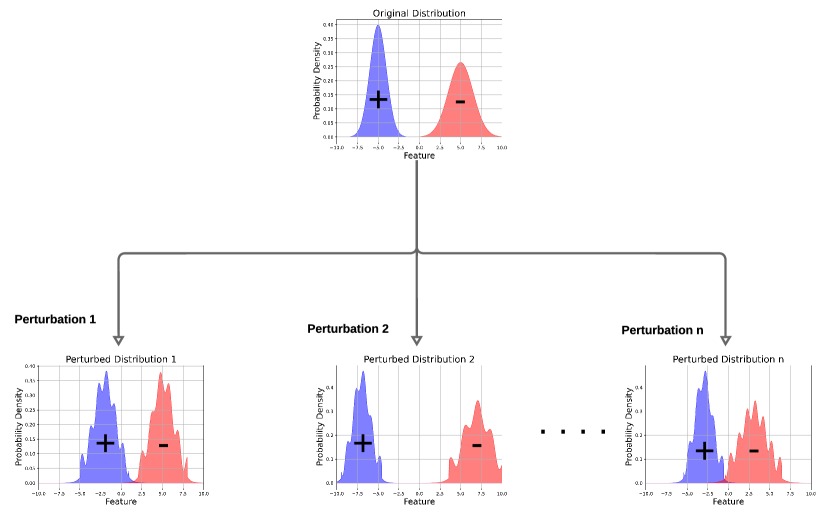
Figure 3: Figure illustrating Distributionally Robust Optimization (DRO). In contrast to ERM which learns a model that minimizes expected loss over original data distribution, DRO learns a model that performs well simultaneously on several perturbed versions of the original data distribution.

In DRO, we assume that a “worst-case” data distribution shift may occur, which can harm a model’s performance. So, DRO optimizes the loss for samples in that “worst-case” distribution, making the model robust to perturbations (see Figure 3 for illustration). Letting $D$ be a divergence that measures the distance between two probability distributions, the population and empirical DRO risks w.r.t $D$ are defined as

$$R_{D}(\theta)\coloneqq\sup_{P^{\prime}:D(P^{\prime}||P_{\text{data}})\leq\rho}\mathbb{E}_{P^{\prime}}[\ell(z,\theta)],\quad\widehat{R}_{D,n}(\theta)\coloneqq\sup_{P^{\prime}:D(P^{\prime}||\widehat{P}_{\text{data}})\leq\rho}\mathbb{E}_{P^{\prime}}[\ell(z,\theta)].$$

Here, $\rho$ is the perturbation radius. Popular choices for $D$ include $f$-divergences, which are defined as $D_{f}(Q||P)=\mathbb{E}_{P}[f(dQ/dP)]$ for some convex function $f:\mathbb{R}_{+}\to\mathbb{R}$. We note that many popular divergences, such as Kullback–Leibler (KL) divergence ($f(x)=x\log{x}$), Total Variation distance ($f(x)=\frac{1}{2}|x-1|$), and $\chi^{2}$-divergence ($f(x)=(x-1)^{2}$), fall into this category.

Generalization Properties.

Models learned using ERM can suffer from poor generalization (i.e., performance on unseen data) in high-variance settings. To see this, consider the following well-known generalization guarantee that holds with high probability for any $\theta\in\Theta$ (Wainwright, 2019)

$$R(\theta)\leq\widehat{R}_{n}(\theta)+c_{1}\sqrt{\frac{\text{Var}_{\widehat{P}_{\text{data}}}(\ell(z;\theta))}{n}}+\frac{c_{2}}{n}.$$ (1)

Here, $c_{1},c_{2}>0$ are constants, and $\text{Var}_{P}(\ell(z;\theta))$ is the variance of $\ell(z;\theta)$ w.r.t distribution $P$. Such bounds hold under certain regularity conditions on $\ell$ and $\Theta$. While ERM minimizes the first term in the RHS above, it totally ignores the second term involving the variance. Consequently, in high-variance and/or small $n$ settings where $R(\theta)$ and $\widehat{R}_{n}(\theta)$ are far away from each other, ERM tends to have poor generalization guarantees. A natural technique to address this issue is to learn models that consider the bias-variance trade-off and minimize the following objective.

$$\min_{\theta\in\Theta}\widehat{R}_{n}(\theta)+c_{1}\sqrt{\frac{\text{Var}_{\widehat{P}_{\text{data}}}(\ell(z;\theta))}{n}}.$$

However, minimizing this objective is computationally intractable even when the loss $\ell$ is convex in $\theta$, as the overall objective is non-convex. Recent works have made an interesting connection between the above objective and DRO to address this issue. Specifically, when $D$ is an $f$-divergence, the following result holds with high probability, whenever the perturbation radius $\rho=\frac{c}{n}$, for some appropriately chosen constant $c>0$ (Lam, 2019; Namkoong & Duchi, 2017)

$$\widehat{R}_{D,n}(\theta)=\widehat{R}_{n}(\theta)+c_{1}\sqrt{\frac{\text{Var}_{\widehat{P}_{\text{data}}}(\ell(z;\theta))}{n}}+\frac{c_{3}}{n}\quad\forall\theta\in\Theta.$$

Together with Equation 1, the above result shows that the empirical DRO risk $\widehat{R}_{D,n}(\theta)$ is an upper bound of the population risk $R(\theta)$ at any $\theta\in\Theta$. Consequently minimizing the DRO risk achieves a better bias-variance trade-off than ERM, and leads to models with better generalization guarantees.

3.2 Stochastic Re-weighted Gradient Descent (RGD)

The above discussion motivates the use of DRO risk for learning models, especially in high variance and low sample regime. We now derive our RGD algorithm as a technique to minimize the empirical DRO risk $\widehat{R}_{D,n}$, and to learn models with better generalization guarantees than ERM. Specifically, we consider KL divergence-based DRO, where one adds perturbations to create data distributions that are close to the original data distribution in the KL divergence metric, and learn a model with best performance over all possible perturbations. The following proposition derives the dual representation of the KL divergence-DRO objective, the proof of which can be found in Appendix A.1.

Proposition 3.1.

Consider DRO with KL-divergence-based uncertainty set. Assume that the data set $\{z_{i}\}_{i=1}^{n}$ is comprised of unique points (i.e, no repeated data points). Then $\min_{\theta\in\Theta}\widehat{R}_{D,n}$ can be rewritten as

$$\min_{\theta\in\Theta}\frac{1}{\gamma}\log{\mathbb{E}_{\widehat{P}_{\text{data}}}[e^{\gamma\ell(z;\theta)}]},$$

for some constant $\gamma>0$ that is independent of $\theta$.

Algorithm 1 Re-weighted Gradient Descent (RGD)

1:Input: Data $\{z_{i}\}_{i=1}^{n},$ learning rate sequence $\{\eta_{t}\}_{t=1}^{T}$, number of iterations $T$, loss function $\ell$, re-weighting function $g$, mini-batch size $B$

2:for $t=0\dots T-1$ do

3:   Sample minibatch $\{z_{i}\}_{i=1}^{B}$

4:   Compute losses for points in the minibatch: $\ell_{i}\leftarrow\ell(z_{i};\theta_{t}),\ \forall i\in{1\dots B}$

5:   Compute per-sample weights using our proposed approach: $w_{i}\leftarrow g(\ell_{i})\ \forall i\in{1\dots B}$

6:   Compute the weighted pseudo-gradient: $v_{t}\leftarrow\frac{1}{B}\sum_{i=1}^{B}w_{i}\nabla_{\theta}\ell(z_{i};\theta_{t})$

7:   Update model parameters: $\theta_{t+1}\leftarrow\Pi_{\Theta}(\theta_{t}-\eta_{t}v_{t})$

8:end for

Equipped with the dual representation, we now derive our RGD algorithm. Observe that minimizing $\widehat{R}_{D,n}$ is equivalent to minimizing $\mathbb{E}_{\widehat{P}_{\text{data}}}[e^{\gamma\ell(z;\theta)}].$ Using SGD on this objective gives us the update:

$$\theta_{t+1}\leftarrow\Pi_{\Theta}\left(\theta_{t}-\gamma\eta_{t}\frac{1}{B}\sum_{i-1}^{B}e^{\gamma\ell(z_{i};\theta_{t})}\nabla_{\theta_{t}}\ell(z_{i};\theta_{t})\right).$$

Here $\Pi_{\Theta}$ is the projection onto the feasible set $\Theta$. The following proposition shows that this update rule converges to the minimum of $\widehat{R}_{D,n}$ under certain conditions on $\ell(z;)$. The proof, given in Appendix A.2 follows from an application of (Shamir & Zhang, 2013, Theorem 2).

Proposition 3.2.

Assume that $\Theta$ is a convex and compact set. For all data points $z$ suppose that $\ell(z;\cdot)$ is convex, continuously differentiable and bounded in the range $[-M,M]$, and $\nabla\ell(z;\cdot)$ is uniformly bounded over the set $\Theta$. Let the step-size sequence $(\eta_{t})_{t}$ be such that $\eta_{t}=\frac{C}{\sqrt{t}}$ $\forall$ $1\leq t\leq T$ or $\eta_{t}=\frac{C}{\sqrt{T}}$ $\forall$ $1\leq t\leq T$. Then,

$$\mathbb{E}_{\theta_{T}}\frac{1}{\gamma}\log{\mathbb{E}_{\widehat{P}_{\text{data}}}[e^{\gamma\ell(z;\theta_{T})}]}-\min_{\theta\in\Theta}\frac{1}{\gamma}\log{\mathbb{E}_{\widehat{P}_{\text{data}}}[e^{\gamma\ell(z;\theta)}]}=O\left(\frac{\log T}{\sqrt{T}}\right)$$

This shows that choosing the re-weighting function $g(u)$ in Algorithm 1 as $e^{\gamma u}$ (for some appropriate choice of $\gamma$) leads to robust models with better generalization guarantees. This is the choice of $g$ we use in our paper. One thing to note here is that, even though the proposition is specific to SGD, it can be easily extended to other optimization techniques such as Adam.

Implementation Details. In our experiments, when computing per-sample weights, we clip the loss $\ell$ at some constant $\tau>0$; that is, we use $g(u)=e^{\gamma\min(u,\tau)}$. We observed this clipping to help stabilize the training in the presence of outliers. Furthermore, we always set $\gamma=1/(\tau+1),$ where $\tau$ is the clipping threshold. Even with this fixed choice of $\gamma$, our algorithm provides a significant boost in performance over vanilla optimization techniques.

Choice of divergences. One could rely on other divergences instead of the KL-divergence we used in the above derivation. From a theoretical perspective, DRO with many $f$-divergences (KL, reverse KL, chi-squared etc.) provides an upper bound on the true population risk (Lam, 2016; Duchi et al., 2021). For example, using $\chi^{2}$-divergence ($f(x)=(x-1)^{2}$) gives us the following re-weighting function for positive loss functions: $g(u)=u+\tau$. Using reverse KL-divergence ($f(x)=-\log{x}$) gives us the following re-weighting function $g(u)=\frac{1}{\tau-u}$ for some appropriate choice of $\tau$ (see Appendix A.3 for more details). Observe that the reverse KL-divergence based weighting function is much more aggressive in up-weighting high loss points than KL-divergence based weighting function. For clarity and future references across the paper, we will denote the approach with $g(u)=u+\tau$ as RGD-x, $g(u)=\frac{1}{\tau-u}$ as RGD-1, and $g(u)=e^{\min(u,\tau)/(\tau+1)}$ as RGD-exp. While all of these provided a performance boost over ERM (see Appendix C), KL-divergence based reweighting has better performance than reverse KL, chi-squared divergences. However, the current theoretical understanding of DRO doesn’t explain this nuanced behavior and we believe that this is an interesting direction for future research. From a practitioner perspective, the choice of $f$-divergence could be treated as a hyper-parameter which could be tuned using cross-validation/hold-out set validation.

4 Toy Examples

In this section, we perform two experiments to study the robustness properties our proposed approach. Linear Regression: We consider a linear regression problem where the covariates $x$ are sampled from the set $\{h(0),\dots h(9)\}$. Here $h(\cdot)$ is a one-hot encoder that maps its inputs to a 10-dimensional vector. The label $y$ is generated according to the following linear model: $y=x^{T}\theta^{*}$, where $\theta^{*}\in\mathbb{R}^{10}$ is the regression vector which is sampled from a standard normal distribution. We construct an imbalanced dataset of tuples $\{(x_{i},y_{i})\}_{i=1}^{n}$ by taking 50 occurrences of the covariates $\{h(0)\dots h(4)\}$ and only one occurrence of the remaining five covariates. We consider two algorithms for learning the unknown parameter vector $\theta^{*}$: (i) SGD on the mean squared error in predictions (MSE) (ii) RGD on the MSE loss. We set the step size to be $4$ for both algorithms and plot the evolution of MSE and the Euclidean distance between the iterates ($\theta$) and the true parameter ($\theta^{*}$) (Figure 1). It can be seen that our method achieves better performance due to prioritization of samples with higher loss, which corresponds to rare directions in the dataset.

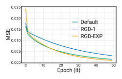
(a) MSE loss convergence

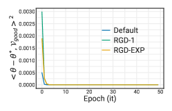
(b) L2 Distance (Frequent feature)

(c) L2 Distance (Rare feature)

Figure 1: Figure 1(a) showing the convergence of SGD, RGD algorithms for estimating the linear regression parameter. The L2 distance between the iterates ($\theta$) and the true parameter $\theta^{*}$ is studied in Figures 1(b) and 1(c). Specifically, Figure 1(b) depicts the squared error in the frequently appearing directions, where all the techniques perform equally well. However, when it comes to learning rare directions, our proposed approach is much better (Figure 1(c)).

Class Imbalance and Fairness: An interesting byproduct of RGD is that it leads to models that are robust to class imbalance where certain classes in the dataset are underrepresented. This is because DRO upweights rare points with high loss (Namkoong & Duchi, 2017). To demonstrate this, we test our method on the imbalanced CIFAR dataset. Our method achieves superior performance compared to specialized techniques like class-balanced loss (Cui et al., 2019) and focal loss (Lin et al., 2017) that are specifically designed to tackle this problem, by a significant margin of $2$-$4\%$ (see Figure 2). Refer to Appendix D for more details about the experiment.

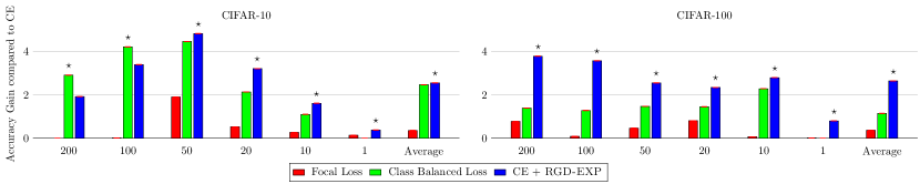
Figure 2: Experiment comparing RGD with baseline cross entropy Loss (CE), focal loss and class-balanced loss. $x$-axis represents the imbalance factor in the dataset.

5 Experiments

In this section, we present large scale experiments to show that our proposed solution can be widely applied across tasks such as supervised learning, meta learning and across domains such as vision, language. Due to space constraints, details regarding hyperparameter tuning are described in Appendix Reproducibility Statement. Additional experimental results on large-scale tasks including EfficientNet finetuning, LLM pretraining are presented in Appendix D.

5.1 Supervised Learning

This section studies our approach when applied on standard supervised learning tasks such as BERT finetuning on GLUE benchmark, and Imagenet-1K classification. We use a base model of ViT-S for the latter task. Table 1 depicts our results from this experiment. On GLUE tasks, our RGD algorithm outperforms the baseline by +1.94%. On Imagenet-1K, we show a +1.01% improvement over baseline with the off-the-hat addition of the RGD reweighing and no hyperparameter search, or additional complexity in terms of compute: memory and time. Additional experiments on supervised learning are discussed in Appendix D.1.

Table 1: Performance of RGD for various Supervised Learning tasks. We depict the performance on GLUE benchmark for bert-base-uncased models. For Vision tasks such as ImageNet-1K, we report improvements over the base ViT-S model.

	MNLI	QQP	QNLI	SST-2	MRPC	RTE	COLA	Avg on GLUE	ImageNet-1K
Default	81.33	89.62	87.93	90.63	89.55	67.19	54.53	80.11	78.1
RGD-exp (Ours)	83.06	91.06	90.35	91.78	88.28	71.48	58.56	82.05	79.11 $\pm$ 0.12

5.2 Tabular Classification

This work considers MET (representation learning with adversarial training) and MET-S (representation learning without adversarial training). The adversarial training adds robustness to the learned representations, thus improving performance. In this experiment, we integrate RGD with MET-S instead of doing adversarial training. This allows us to test the robustness properties of the models trained with RGD. Table 2 and Table 3 shows gains on multiple tabular datasets for the multi-class classification and binary classification tasks. Notably, our approach outperforms previous SOTA in this problem by +1.27%, and +1.5% on the multi-class and binary classification tasks respectively. We refer to Appendix D.3 for a comprehensive comparison with baselines such as Gradient Boosting Decision Trees (Friedman, 2001), VIME (Yoon et al., 2020), SubTab (Ucar et al., 2021), TabNet (Arik & Pfister, 2019), DACL+ (Verma et al., 2021) and many more. Our motivation to experiment on these “permuted” MNIST, “permuted” CIFAR, and “permuted” FMNIST can be traced back to the introduction of these datasets in the works of Yoon et al. (2020); Ucar et al. (2021). Following so, other recent works such as Majmundar et al. (2022) also experiment on these datasets and have become a standard benchmark for tabular classification.

Table 2: Results on standard multi-class tabular datasets (Accuracy): The bottom partition shows results of our method with RGD-exp loss. We show that the addition of our proposed approach significantly outperforms existing methods, as well as SOTA.

Algorithm	FMNIST	CIFAR10	MNIST	CovType	Avg.
MLP	87.62	16.50	96.95	65.47	66.64
RF Breiman (2001)	88.43	42.73	97.62	71.37	75.04
MET Majmundar et al. (2022)	91.68	47.82	99.19	76.71	78.85
MET-S
Default Majmundar et al. (2022)	90.94	48.00	99.01	74.11	78.02
RGD-exp (Ours)	91.54	49.54	99.69	79.72	80.12

Table 3: Results on standard binary-class tabular datasets (AUROC): The bottom partition shows results of our method with RGD loss. We show that the addition of our proposed approach significantly outperforms existing methods, as well as SOTA.

Algorithm	Obesity	Income	Criteo	Thyroid	Avg.
MLP	52.3	89.39	79.82	62.3	70.95
RF Breiman (2001)	64.36	91.53	77.57	99.62	83.27
MET-S
Default Majmundar et al. (2022)	71.84	93.85	86.17	99.81	87.92
RGD-exp (Ours)	76.87	93.96	86.98	99.92	89.43

5.3 Out Of Domain Generalization

In this section, we show that our technique can be used to boost the performance of OOD generalization techniques. We experiment on DomainBed, a standard benchmark used to study the out-of-domain performance of models. More information about the benchmark, the task to solve, and the metric is discussed in Appendix B. The benchmark is notorious since the most basic approach, such as straightforward Empirical Risk Minimization (ERM) as evaluated by Gulrajani & Lopez-Paz (2020), was the SOTA method for a long time. Most new approaches either performed worse than ERM or marginally better. In recent years, breakthroughs such as MIRO (Cha et al., 2022) and FRR (Addepalli et al., 2022) have pushed the problem further by significantly improving the benchmarks. We show that integrating our proposed approach RGD with these approaches (specifically FRR) significantly improves performance (an average of +0.7%). Table 4 illustrates the accuracy performance numbers of a few baseline methods and our proposed approach. A more comprehensive comparison with additional baselines such as IRM (Arjovsky et al., 2019), CORAL (Sun & Saenko, 2016), MTL (Blanchard et al., 2021), SagNet (Nam et al., 2021), and many more in the Table 18. We further depict the environment-wise breakdown of the accuracy of each of the baseline algorithms in Appendix D.5.

Table 4: Results on DomainBed (Model selection: training-domain validation set): The bottom partition shows results of our method with RGD loss. In both cases, with (top) and without (bottom) fixed linear layer, the proposed approach outperforms existing methods, as well as SOTA.

Algorithm	PACS	VLCS	OfficeHome	DomainNet	Avg.
ERM Gulrajani & Lopez-Paz (2020)	85.5 $\pm$ 0.1	77.5 $\pm$ 0.4	66.5 $\pm$ 0.2	40.9 $\pm$ 0.1	67.6
MIRO Cha et al. (2022)	85.4 $\pm$ 0.4	79.0 $\pm$ 0.0	70.5 $\pm$ 0.4	44.3 $\pm$ 0.2	69.8
ERM + FRR-L
Default Addepalli et al. (2022)	85.7 $\pm$ 0.1	76.6 $\pm$ 0.2	68.4 $\pm$ 0.2	44.2 $\pm$ 0.1	68.73
RGD-exp (Ours)	87.6 $\pm$ 0.3	78.6 $\pm$ 0.3	69.8 $\pm$ 0.2	46.00 $\pm$ 0.0	70.48
ERM + FRR
Default Addepalli et al. (2022)	87.5 $\pm$ 0.1	77.6 $\pm$ 0.3	69.4 $\pm$ 0.1	45.1 $\pm$ 0.1	69.90
RGD-exp (Ours)	88.2 $\pm$ 0.2	78.6 $\pm$ 0.3	69.8 $\pm$ 0.2	45.8 $\pm$ 0.0	70.60

5.4 Meta-Learning

In meta-learning, where the objective is to efficiently learn new tasks with limited data, the re-weighing of tasks becomes crucial. While Empirical Risk Minimization (ERM), may perform well on common tasks, it can fail catastrophically on rare and challenging ones. Thus, we apply our re-weighting approach to minimize the worst-case loss over a predefined set of distributions over the tasks. Building upon the experimental results of Kumar et al. (2022), we make comparisons with our MAML + RGD-exp approach as the proposed variant. We evaluate our DRO-inspired reweighting approach not only based on the average performance across tasks but also on the Worst-K% of tasks in a fixed task pool. Our experiments on various benchmarks, including Omniglot 5-way 1-shot, Omniglot 20-way 1-shot, and miniImageNet 5-way 1-shot, demonstrate significant improvements in the Worst-K% metric (Table 5). For example, on Omniglot 20-way 1-shot, our proposed reweighting scheme improves overall performance by 1.83% and the Worst-10% performance by 2.28%. Similarly, on the challenging miniImageNet 5-way 1-shot benchmark, we achieve a substantial improvement of approximately 3% across the board. Further results in this domain are discussed in Appendix D.4.

Table 5: Results on meta-learning datasets. We report the Worst-K% performance as well to help study the performance distribution over all tasks.

Algorithm	Worst 10%	Worst 20%	Worst 30%	Worst 40%	Worst 50%	Overall
Omniglot 5-way 1-shot
MAML	91.71 $\pm$ 0.73	94.16 $\pm$ 0.50	95.41 $\pm$ 0.39	96.22 $\pm$ 0.32	96.76 $\pm$ 0.27	98.38 $\pm$ 0.17
MAML + RGD-exp	92.14 $\pm$ 0.84	94.54 $\pm$ 0.53	95.72 $\pm$ 0.40	96.46 $\pm$ 0.33	96.90 $\pm$ 0.27	98.45 $\pm$ 0.17
Omniglot 20-way 1-shot
MAML	84.33 $\pm$ 0.40	85.86 $\pm$ 0.29	86.92 $\pm$ 0.26	87.73 $\pm$ 0.24	88.42 $\pm$ 0.22	91.28 $\pm$ 0.22
MAML + RGD-exp	86.61 $\pm$ 0.36	88.09 $\pm$ 0.28	89.09 $\pm$ 0.24	89.87 $\pm$ 0.23	90.50 $\pm$ 0.21	93.01 $\pm$ 0.20
miniImageNet 5-way 1-shot
MAML	30.94 $\pm$ 0.70	34.52 $\pm$ 0.62	36.93 $\pm$ 0.57	38.94 $\pm$ 0.55	40.68 $\pm$ 0.53	48.86 $\pm$ 0.62
MAML + RGD-exp	33.33 $\pm$ 0.90	36.67 $\pm$ 0.65	39.12 $\pm$ 0.59	41.20 $\pm$ 0.56	42.96 $\pm$ 0.55	51.21 $\pm$ 0.63

6 Conclusion and Future Work

We introduced a re-weighted gradient descent technique that effectively boosts the performance of deep learning across a wide range of tasks and domains. It is simple to implement and can be seamlessly integrated into existing algorithms with just two lines of code change. Our algorithm is derived from distributionally robust optimization, a known method for improving model generalization.

The RGD algorithm was developed under the assumption that the training data doesn’t have any systematic or adversarial corruptions. Therefore, RGD may not provide performance improvements in scenarios where training data has a high volume of such corruptions. One interesting future direction is to develop variants of RGD that can tolerate corruptions in the training data. Furthermore, in future, we plan to subject our technique to rigorous evaluation on large-scale tasks, such as training Large Language Models (LLMs) and other generative models. By doing so, we aim to gain deeper insights into the utility and limitations of our approach.

Ethical Statement and Broader Impact

Our proposed approach is compatible with any learning objective expressed as an expectation over samples. We showcased its effectiveness with various loss functions, including Mean Square Error, Cross Entropy, and others, outperforming previous state-of-the-art methods considerably. Implementing our approach is straightforward, and it has broad applicability across domains such as Natural Language Processing (NLP), Vision, and Time Series data. As far as we know, no ethical concerns or limitations are associated with this work.

Reproducibility Statement

Our proposed loss function is a single line of change. However, one would have to play around with the learning rate (generally lower than the baseline setting). Our experiments are based on public datasets and open-source code repositories. The proposed final formulation RGD-exp requires one line of code change.

Suppose the per-sample loss is given. Example code for applying RGD-exp is shown below.

⬇

def rgd_e(loss, temp=alpha, reduce=True):

# alpha >0.

out = loss * torch.exp(

torch.clamp(loss.detach(), max=temp) / (temp + 1)

)

return out.sum() / len(out) if reduce else out

The two parameters we tune were $\tau$ and lr. We use a simple grid search for $\tau$ in the order of $[1,\frac{1}{3},\frac{1}{5},\frac{1}{7},\frac{1}{9}]$ across the experiments where the $[denominator-1]$ was used as the clipping factor. This allowed our loss to be bounded between 0,1 and helped fairly compare RGD-1 and RGD-exp. The lr was tuned by a proxy of lr_mult where we scaled the learning rate by a fraction in the range $[0.5,1.5]$.

Appendix

Appendix A Proofs of Section 3

A.1 Proof of Proposition 3.1

Proposition A.1.

Consider DRO with KL-divergence-based uncertainty set. Assume that the data set $(z_{i})_{i=1}^{n}$ is comprised of unique points (i.e, no repeated data points). Then $\min_{\theta\in\Theta}\widehat{R}_{D,n}$ can be rewritten as

$$\min_{\theta\in\Theta}\frac{1}{\gamma}\log{\mathbb{E}_{\widehat{P}_{\text{data}}}[e^{\gamma\ell(z;\theta)}]},$$

for some constant $\gamma>0$ that is independent of $\theta$.

Proof.

Recall the empirical DRO risk $\widehat{R}_{D,n}(\theta)$ is defined as

$$\widehat{R}_{D,n}(\theta)\coloneqq\sup_{P^{\prime}:D(P^{\prime}||\widehat{P}_{\text{data}})\leq\rho}\mathbb{E}_{P^{\prime}}[\ell(z,\theta)]$$

Using Lagrangian duality, we rewrite $\widehat{R}_{D,n}(\theta)$ as

$$\sup_{P^{\prime}:D(P^{\prime}||\widehat{P}_{\text{data}})\leq\rho}\mathbb{E}_{P^{\prime}}[\ell(z,\theta)] =\sup_{P^{\prime}}\inf_{\beta>0}\mathbb{E}_{P^{\prime}}[\ell(z,\theta)]-\beta(D(P^{\prime}||\widehat{P}_{\text{data}})-\rho)$$

$$\stackrel{{\scriptstyle(a)}}{{=}}\sup_{P^{\prime}}\inf_{\beta>0}\mathbb{E}_{P^{\prime}}[\ell(z,\theta)]-\beta(\mathbb{E}_{P^{\prime}}[\log{dP^{\prime}}]+\log{n}-\rho),$$

where $(a)$ follows from our choice of divergence, and the fact that the data points $\{z_{i}\}_{i=1}^{n}$ are all unique (i.e, no repetitions). Observe that the objective in the last expression is concave in $P^{\prime}$ and linear in $\beta$. So the max-min problem above is concave-convex. Using Lagrangian duality to swap the order of min and max, we get

$$\sup_{P^{\prime}:D(P^{\prime}||\widehat{P}_{\text{data}})\leq\rho}\mathbb{E}_{P^{\prime}}[\ell(z,\theta)] =\inf_{\beta>0}\sup_{P^{\prime}}\mathbb{E}_{P^{\prime}}[\ell(z,\theta)]-\beta(\mathbb{E}_{P^{\prime}}[\log{dP^{\prime}}]+\log{n}-\rho).$$

This shows that minimizing $\widehat{R}_{D,n}$ is equivalent to the following problem

$$\inf_{\beta>0,\theta\in\Theta}\sup_{P^{\prime}}\mathbb{E}_{P^{\prime}}[\ell(z,\theta)]-\beta(\mathbb{E}_{P^{\prime}}[\log{dP^{\prime}}]+\log{n}-\rho).$$

For any fixed $\beta,\theta$, the inner supremum is attained at a $P^{\prime}$ that satisfies (see Theorem 1 of Hsieh et al. (2019))

$$P^{\prime}(z)\propto\exp\left(\ell(z,\theta)/\beta\right).$$

This can be derived using the following first order optimality condition: $\forall z,\ell(z,\theta)-\beta\log{P^{\prime}(z)}-\beta=c$ for some constant $c$. Substituting this in the previous equation, we get the following equivalent optimization problem

$$\inf_{\beta>0}\inf_{\theta\in\Theta}\beta\log\mathbb{E}_{P^{\prime}}[e^{\ell(z,\theta)/\beta}]-\beta(\log{n}-\rho).$$

Letting $\gamma^{-1}$ be the minimizer of the outer minimization problem, we get the required result. ∎

A.2 Proof of Proposition 3.2

Proof.

Note that whenever $\ell(z;)$ is convex, so is $f(\theta):=\mathbb{E}_{z\sim\widehat{P}_{\text{data}}}\exp(\gamma\ell(z;))$. It is easy to check that the function $f$ and the constraint set $\Theta$ satisfy the conditions in (Shamir & Zhang, 2013, Theorem 2). From this, we conclude that:

$$\mathbb{E}_{\theta_{T}}f(\theta_{T})-\inf_{\theta\in\Theta}f(\theta)=O\left(\frac{\log T}{\sqrt{T}}\right)$$ (2)

The proof of equation 2 for the step size sequence $\eta_{t}=\frac{C}{\sqrt{t}}$ follows from the statement of (Shamir & Zhang, 2013, Theorem 2). The case of the constant step-size $\eta_{t}=\frac{C}{\sqrt{T}}$ follows by a simple modification of the proof of (Shamir & Zhang, 2013, Theorem 2) where we substitute the appearance of $1/\sqrt{t}$ due to the step size with $1/\sqrt{T}$. We now convert the guarantees in Equation 2 to guarantees in terms of $\log{f(\theta)}.$ Let $\theta^{*}\in\arg\inf_{\theta\in\Theta}f(\theta)$. By our assupmption, $\ell(z;)$ is bounded above and below. So $\log f(\theta_{T})-\log f(\theta^{*})\leq\bar{C}(f(\theta_{T})-f(\theta^{*}))$ for some $\bar{C}$. Combining this with equation 2, we conclude the statement of the proposition. ∎

A.3 Other Divergences

$\chi^{2}$-divergence.

Consider $\chi^{2}$-divergence which is defined as

$$D(P^{\prime}||P)=\mathbb{E}_{P}\left[\left(\frac{dP^{\prime}}{dP}-1\right)^{2}\right].$$

We now follow a similar argument as in the proof of Proposition 3.1 to derive an equivalent expression for the DRO objective. We have

$$\sup_{P^{\prime}:D(P^{\prime}||\widehat{P}_{\text{data}})\leq\rho}\mathbb{E}_{P^{\prime}}[\ell(z,\theta)] =\sup_{P^{\prime}}\inf_{\beta>0}\mathbb{E}_{P^{\prime}}[\ell(z,\theta)]-\beta(D(P^{\prime}||\widehat{P}_{\text{data}})-\rho)$$

$$\stackrel{{\scriptstyle(a)}}{{=}}\sup_{P^{\prime}}\inf_{\beta>0}\mathbb{E}_{P^{\prime}}[\ell(z,\theta)]-\beta(\mathbb{E}_{P^{\prime}}[dP^{\prime}/d\widehat{P}_{\text{data}}]-1-\rho)$$

$$\stackrel{{\scriptstyle(b)}}{{=}}\sup_{P^{\prime}}\inf_{\beta>0}\mathbb{E}_{P^{\prime}}[\ell(z,\theta)]-\beta(n\mathbb{E}_{P^{\prime}}[dP^{\prime}]-1-\rho)$$

$$\stackrel{{\scriptstyle(c)}}{{=}}\inf_{\beta>0}\sup_{P^{\prime}}\mathbb{E}_{P^{\prime}}[\ell(z,\theta)]-\beta(n\mathbb{E}_{P^{\prime}}[dP^{\prime}]-1-\rho),$$

where $(a),(b)$ follow from the definition of the divergence and $(c)$ follows from Lagrangian duality. Now, consider the DRO optimization problem

$$\sup_{P^{\prime}:D(P^{\prime}||\widehat{P}_{\text{data}})\leq\rho}\mathbb{E}_{P^{\prime}}[\ell(z,\theta)] =\inf_{\beta>0,\theta\in\Theta}\sup_{P^{\prime}}\mathbb{E}_{P^{\prime}}[\ell(z,\theta)]-\beta(n\mathbb{E}_{P^{\prime}}[dP^{\prime}]-1-\rho).$$

Suppose the loss $\ell$ is positive. For any fixed $\theta,\beta$, the inner supremum in the above optimization problem is attained at a $P^{\prime}$ that satisfies

$$P^{\prime}(z)\propto\left(\ell(z,\theta)/\beta n+1\right).$$

This follows from the first order optimality conditions. This gives rise to the re-weighting scheme $g(x)=x+\tau$, for some appropriately chosen $\tau$.

Reverse KL divergence.

The reverse KL-divergence is defined as

$$D(P^{\prime}||P)=\mathbb{E}_{P}\left[-\log{\frac{dP^{\prime}}{dP}}\right].$$

Using similar arguments as above, we can rewrite the DRO optimization problem as

$$\sup_{P^{\prime}:D(P^{\prime}||\widehat{P}_{\text{data}})\leq\rho}\mathbb{E}_{P^{\prime}}[\ell(z,\theta)] =\inf_{\beta>0,\theta\in\Theta}\sup_{P^{\prime}}\mathbb{E}_{P^{\prime}}[\ell(z,\theta)]+\beta(\mathbb{E}_{P}[\log{dP^{\prime}}]-\log{n}-\rho).$$

For any fixed $\theta,\beta$, the inner supremum in the above optimization problem is attained at a $P^{\prime}$ that satisfies

$$P^{\prime}(z)\propto\frac{1}{\tau-\ell(z,\theta)},$$

for some appropriate $\tau$. This gives rise to the re-weighting scheme $g(x)=1/(\tau-x)$. We call this algorithm RGD-1. In practice, we modify this re-weighting function It can be implemented using the following pseudocode.

⬇

def rgd_t(loss, temp=alpha, reduce=True):

# alpha >0.

out = loss * (

(1 - torch.clamp(loss.detach(), max=temp) / (temp + 1)) ** (-1)

)

return out.sum() / len(out) if reduce else out

Appendix B DomainBed Benchmark

In this section, we describe the DomainBed benchmark, a challenging benchmark used to study the out-of-domain generalization capabilities of our model. To briefly explain, consider the dataset PACS, which consists of Photos, Art, cartoons, and sketches of the same set of classes (for instance, dogs and cats, amongst others). The goal of the task is to learn from three of these domains and evaluate the performance of the left-out domain (similar to a k-fold cross-validation). By doing so, we can assess the out-of-domain generalization performance of our models. In general, the metric used in this domain involves taking an average of the performance of the different k-fold splits. More information about this benchmark is available at Gulrajani & Lopez-Paz (2020).

Appendix C Choice of divergence in RGD

RGD-1is a more aggressive weighing scheme in comparison to RGD-exp. This is fairly simple to show if you re-write both the reweighting techniques using Taylor series expansion. RGD-1  multiplies the loss $l$ with $(1+l+l^{2}+\dots)$. Whereas, RGD-exp multiplies the loss $l$ with $(1+l+l^{2}/2!+l^{3}/3!+\dots)$. RGD-1 is a more aggressive weighing scheme than RGD-exp, and the choice between the two schemes should depend on the problem. Some preliminary results on the class imbalance setting is depicted in Table 6.

Table 6: Test Accuracy of ResNet-32 on Long-Tailed CIFAR-10, and CIFAR-100 dataset.

Dataset	CIFAR-10							CIFAR-100
Loss / Imbalance Factor	200	100	50	20	10	1	Avg.	200	100	50	20	10	1	Avg.
Cross Entropy (CE)
Default	65.98	70.36	74.81	82.23	86.39	92.89	78.78	34.84	38.32	43.85	51.14	55.71	70.50	49.06
RGD-1 (Ours)	64.16	72.56	77.86	83.88	86.84	92.99	79.72	36.22	39.87	43.74	51.86	56.9	70.80	49.90
RGD-exp (Ours)	67.90	73.75	79.63	85.44	88.00	93.27	81.33	38.62	41.89	46.40	53.48	58.5	71.30	51.70

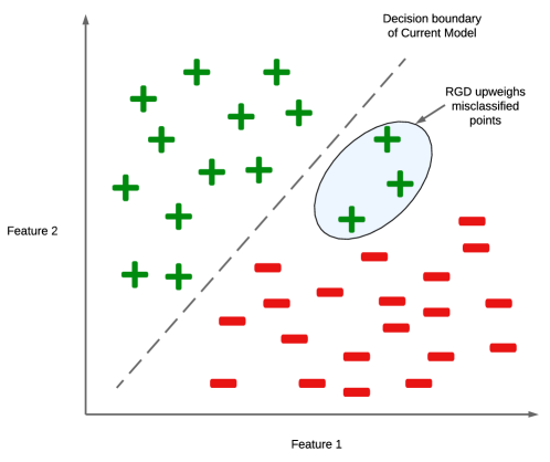
Figure 4: Figure illustrating the intuitive idea behind the working of RGD in the binary classification setting. RGD upweights the points which have high losses - points which have been misclassified by the model.

Appendix D Additional Results

This section briefly discusses more elaborated tables and findings from our research.

D.1 Vanilla Classification

This section briefly discusses a few additional results from our experiments on Vanilla classification. Table 7 depicts the performance of our other variant RGD-1 in comparison to the baseline approach. Furthermore, we also show fine-tuning improvements of EfficientNet-v2-l over various tasks such as Cars and Food101 as depicted in Table 8. Furthermore, we also demonstrate that our proposed approach is simple and shows significant improvements, not only for SOTA approaches but also basic MLP procedures as depicted in Table 12, Table 13, and Table 14. These tables help showcase that the simple addition of our proposed approach does show significant improvements of +2.77% (in accuracy) on multi-class and +1.77% (in AUROC) on binary class tasks respectively.

Table 7: Additional Ablation study to showcase the gain achieved by using RGD for various tasks in GLUE benchmark for bert-base-uncased.

bert-base-uncased	MNLI	QQP	QNLI	SST-2	MRPC	RTE	COLA	Avg
Default	81.33	89.62	87.93	90.63	89.55	67.19	54.53	80.11
RGD-1 (Ours)	82.97	89.87	90.79	91.28	88.54	71.23	59.28	81.97
RGD-exp (Ours)	83.06	91.06	90.35	91.78	88.28	71.48	58.56	82.05

Table 8: Ablation study to showcase the gain achieved by using RGD for various tasks in Vision benchmarks for ViT-S on Imagenet-1K and EfficientNet-v2-l on Finetuning tasks.

	Imagenet-1K	Cars-FineTuning	Food101-FineTuning
Default	78.1	92.03	92.65
RGD-exp (Ours)	79.0	92.62	92.75

D.2 Class Imbalance Experiments

This section briefly discusses additional results from our experiments on the Class Imbalance domain with datasets such as CIFAR-10 and CIFAR-100. It is well known that DRO outputs models with good tail performance (Duchi & Namkoong, 2018). Since RGD directly solves the DRO objective, our models are also naturally endowed with this property. To demonstrate this, we extend our experiments on linear regression to a more realistic image dataset, where some classes appear very rarely in the data set while some appear very frequently. We use the Long-Tailed CIFAR dataset, where we reduce the number of training samples per class according to an exponential function as proposed by Cui et al. (2019). We define the imbalance factor of a dataset as the number of training samples in the largest class divided by the smallest. Similar to the works of Shu et al. (2019), we use a ResNet-32 architecture for training. Apart from Cross Entropy loss, we also include Focal Loss (Lin et al., 2017) and Class Balanced Loss (Cui et al., 2019) as additional baselines. We also experimented with the long-tailed CIFAR-100 dataset and showed that our proposed approach could again show significant improvements. Figure 2 illustrates the performance of our approach in comparison to other state-of-the-art methods. Overall, in comparison to the SOTA approach in this task (Class Balanced Loss), our proposed approach brings about an improvement of +0.79%. A more comprehensive comparison with additional state-of-the-art baselines such as L2RW (Ren et al., 2018), and Meta-Weight-Net (Shu et al., 2019) is illustrated in Table 10. Although these models use additional data as a meta-validation-set, our proposed approach outperforms L2RW and is roughly competitive with the Meta-Weight-Net model.

Table 9 depicts the accuracy metric of models on various levels of the imbalance factor. From Table 9, we show that our proposed approach RGD-exp outperforms other baselines such as Focal Loss and Class Balanced Loss by +0.79%. Furthermore, when models are trained on additional data, either by fine-tuning or by using a meta-learning framework to learn weights (such as Meta-Weight-Net and L2RW), we show that our proposed approach is competitively similar (-0.22%). Table 10 illustrates this analysis further. The performance metrics of the baseline approaches were taken from Shu et al. (2019). Additional comparisons against other losses, such as cross-entropy with label smoothing and large margin softmax loss, are shown in Table 11.

Table 9: Test Accuracy of ResNet-32 on Long-Tailed CIFAR-10, and CIFAR-100 dataset.

Dataset	CIFAR-10							CIFAR-100
Loss / Imbalance Factor	200	100	50	20	10	1	Avg.	200	100	50	20	10	1	Avg.
Focal Loss Lin et al. (2017)	65.29	70.38	76.71	82.76	86.66	93.03	79.14	35.62	38.41	44.32	51.95	55.78	70.52	49.43
Class Balanced Loss Cui et al. (2019)	68.89	74.57	79.27	84.36	87.49	92.89	81.25	36.23	39.60	45.32	52.59	57.99	70.50	50.21
Cross Entropy (CE)
Default	65.98	70.36	74.81	82.23	86.39	92.89	78.78	34.84	38.32	43.85	51.14	55.71	70.50	49.06
RGD-1 (Ours)	64.16	72.56	77.86	83.88	86.84	92.99	79.72	36.22	39.87	43.74	51.86	56.9	70.80	49.90
RGD-exp (Ours)	67.90	73.75	79.63	85.44	88.00	93.27	81.33	38.62	41.89	46.40	53.48	58.5	71.30	51.70

Table 10: Test Accuracy of ResNet-32 on Long-Tailed CIFAR-10, and CIFAR-100 dataset. We use the symbol $\star$ to denote approaches that use additional data (as the meta-dataset). We use $\underline{underline}$ symbol to depict performances which are second-best across baselines. Our experiments show that we can get competitively similar performance to such models as well without training a second neural network.

Dataset	CIFAR-10							CIFAR-100
Loss / Imbalance Factor	200	100	50	20	10	1	Avg.	200	100	50	20	10	1	Avg.
Fine-tuning $\star$	66.08	71.33	77.42	83.37	86.42	93.23	79.64	38.22	41.83	46.40	52.11	57.44	70.72	51.12
L2RW Ren et al. (2018) $\star$	66.51	74.16	78.93	82.12	85.19	89.25	77.69	33.38	40.23	44.44	51.64	53.73	64.11	47.92
Meta-Weight-Net Shu et al. (2019) $\star$	68.91	75.21	80.06	84.94	87.84	92.66	81.60	37.91	42.09	46.74	54.37	58.46	70.37	51.65
Cross Entropy (CE)
Default	65.98	70.36	74.81	82.23	86.39	92.89	78.78	34.84	38.32	43.85	51.14	55.71	70.50	49.06
RGD-1 (Ours)	64.16	72.56	77.86	83.88	86.84	92.99	79.72	36.22	39.87	43.74	51.86	56.9	70.80	49.90
RGD-exp (Ours)	67.90	73.75	79.63	85.44	88.00	93.27	81.33	38.62	41.89	46.40	53.48	58.5	71.30	51.70

Table 11: Additional Ablation study comparing with Label smoothing and Large Margin Softmax Loss. Test Accuracy of ResNet-32 on Long-Tailed CIFAR-10, and CIFAR-100 dataset.

Dataset	CIFAR-10							CIFAR-100
Loss / Imbalance Factor	200	100	50	20	10	1	Avg.	200	100	50	20	10	1	Avg.
Cross Entropy (CE)
+ Label Smoothing	61.22	73.80	77.95	84.40	86.96	92.18	79.42	37.14	41.05	44.76	50.67	57.74	70.97	50.39
+ Large Margin Softmax (LMS)	68.67	72.78	78.84	85.23	88.26	92.75	81.09	36.77	40.38	45.24	51.25	56.9	71.01	50.26
RGD-exp (Ours)	67.90	73.75	79.63	85.44	88.00	93.27	81.33	38.62	41.89	46.40	53.48	58.5	71.30	51.70

D.3 Tabular Classification

This section discusses a few additional results from our experiments on Tabular classification. Table 15 depicts our proposed approach’s accuracy compared to other baselines on multi-class tabular datasets. Our method outperforms previous SOTA in this problem by +1.27%. Furthermore, Table 16 illustrates the AUROC score of our proposed approach in comparison to state-of-the-art baselines on binary-class tabular datasets. Our approach shows an improvement of +1.5% in this setting as well. The performance metrics of the baseline approaches were taken from Majmundar et al. (2022).

Table 12: Results on standard multi-class tabular datasets (Accuracy): The bottom partition shows results of our method with RGD-exp loss. We show that the addition of our proposed approach significantly outperforms the base MLP model.

Algorithm	FMNIST	CIFAR10	MNIST	CovType	Avg.
Default Majmundar et al. (2022)	87.62	16.50	96.95	65.47	66.64
RGD-1 (Ours)	88.52	20.31	97.86	68.81	68.875
RGD-exp (Ours)	89.03	21.32	97.57	69.73	69.41

Table 13: Results on standard binary-class tabular datasets (Accuracy): The bottom partition shows results of our method with RGD-exp loss. We show that the addition of our proposed approach significantly outperforms the base MLP model.

Algorithm	Obesity	Income	Criteo	Thyroid	Avg.
Default	58.1	84.36	74.28	50	66.69
RGD-1 (Ours)	59.12	84.5	75.06	57.3	69
RGD-exp (Ours)	58.83	85.5	75.87	56.04	69.1

Table 14: Results on standard binary-class tabular datasets (AUROC): The bottom partition shows results of our method with RGD-exp loss. We show that the addition of our proposed approach significantly outperforms the base MLP model.

Algorithm	Obesity	Income	Criteo	Thyroid	Avg.
MLP	52.3	89.39	79.82	62.3	70.95
RGD-1 (Ours)	54.31	91.1	79.85	62.25	71.88
RGD-exp (Ours)	55.96	90.8	80.1	64	72.72

Table 15: Results on standard multi-class tabular datasets (Accuracy): The bottom partition shows results of our method with RGD loss. We show that the addition of our proposed approach significantly outperforms existing methods, as well as SOTA.

Algorithm	FMNIST	CIFAR10	MNIST	CovType	Avg.
MLP	87.62	16.50	96.95	65.47	66.64
RF Breiman (2001)	88.43	42.73	97.62	71.37	75.04
GBDT Friedman (2001)	88.71	45.7	100	72.96	76.84
RF-G Rahimi & Recht (2008)	89.84	29.32	97.65	71.57	72.10
MET-R Majmundar et al. (2022)	88.84	28.94	97.44	69.68	71.23
VIME Yoon et al. (2020)	80.36	34.00	95.77	62.80	68.23
DACL+ Verma et al. (2021)	81.40	39.70	91.40	64.23	69.18
SubTab Ucar et al. (2021)	87.59	39.34	98.31	42.36	66.90
TabNet Arik & Pfister (2019)	88.18	33.75	96.63	65.13	70.92
MET Majmundar et al. (2022)	91.68	47.82	99.19	76.71	78.85
MET-S
Default Majmundar et al. (2022)	90.94	48.00	99.01	74.11	78.02
RGD-1 (Ours)	91.12	49.17	99.28	79.41	79.75
RGD-exp (Ours)	91.54	49.54	99.69	79.72	80.12

Table 16: Results on standard binary-class tabular datasets (AUROC): The bottom partition shows results of our method with RGD loss. We show that the addition of our proposed approach significantly outperforms existing methods, as well as SOTA.

Algorithm	Obesity	Income	Criteo	Thyroid	Avg.
MLP	52.3	89.39	79.82	62.3	70.95
RF Breiman (2001)	64.36	91.53	77.57	99.62	83.27
GBDT Friedman (2001)	64.4	92.5	78.77	99.34	83.75
RF-G Rahimi & Recht (2008)	54.45	90.09	80.32	52.65	69.37
MET-R Majmundar et al. (2022)	53.2	83.54	79.17	82.03	74.49
VIME Yoon et al. (2020)	57.27	87.37	74.28	94.87	78.45
DACL+ Verma et al. (2021)	61.18	89.01	75.32	86.63	78.04
SubTab Ucar et al. (2021)	64.92	88.95	76.57	88.93	79.00
TabNet Arik & Pfister (2019)	69.40	77.30	80.91	96.98	81.15
MET-S
Default Majmundar et al. (2022)	71.84	93.85	86.17	99.81	87.92
RGD-1 (Ours)	76.23	93.90	86.92	99.82	89.22
RGD-exp (Ours)	76.87	93.96	86.98	99.92	89.43

D.4 Meta-Learning

This section discusses some additional results from our experiments in the meta-learning domain. Table 17 depicts a complete table and comparison of our proposed approach on the MAML baseline compared to others. Overall, we notice improvement across the board, especially in the outliers, as shown in the Worst-k% metrics. Note that although our RGD has been applied on MAML (Finn et al., 2017) in our current experiments, our approach is analogous to the model and can be extended to other meta-learning techniques such as Protonet (Snell et al., 2017), CNAPs (Requeima et al., 2019), etc. as well.

Table 17: Results on meta-learning datasets. We report the Worst-K% performance as well to help study the performance distribution over all tasks. Overall, we expect our reweighting scheme to give more importance to those tasks which are difficult and rare. We show that the addition of our proposed approach significantly outperforms existing methods as shown in Omniglot 5-way 1-shot, as well as miniImageNet 5-way 1-shot setting.

Algorithm	Worst 10%	Worst 20%	Worst 30%	Worst 40%	Worst 50%	Overall
Omniglot 5-way 1-shot
MAML	91.71 $\pm$ 0.73	94.16 $\pm$ 0.50	95.41 $\pm$ 0.39	96.22 $\pm$ 0.32	96.76 $\pm$ 0.27	98.38 $\pm$ 0.17
Reptile	82.78 $\pm$ 0.85	86.22 $\pm$ 0.64	88.33 $\pm$ 0.54	89.79 $\pm$ 0.48	90.93 $\pm$ 0.43	94.64 $\pm$ 0.32
Protonet	88.72 $\pm$ 0.99	92.24 $\pm$ 0.70	93.95 $\pm$ 0.54	95.06 $\pm$ 0.44	95.79 $\pm$ 0.38	97.82 $\pm$ 0.23
Matching Networks	79.70 $\pm$ 0.95	84.01 $\pm$ 0.78	86.78 $\pm$ 0.68	88.83 $\pm$ 0.62	90.41 $\pm$ 0.56	94.71 $\pm$ 0.39
MAML + RGD-exp	92.14 $\pm$ 0.84	94.54 $\pm$ 0.53	95.72 $\pm$ 0.40	96.46 $\pm$ 0.33	96.90 $\pm$ 0.27	98.45 $\pm$ 0.17
Omniglot 20-way 1-shot
MAML	84.33 $\pm$ 0.40	85.86 $\pm$ 0.29	86.92 $\pm$ 0.26	87.73 $\pm$ 0.24	88.42 $\pm$ 0.22	91.28 $\pm$ 0.22
Reptile	83.13 $\pm$ 0.42	84.71 $\pm$ 0.31	85.77 $\pm$ 0.26	86.60 $\pm$ 0.24	87.30 $\pm$ 0.23	90.09 $\pm$ 0.22
Protonet	87.19 $\pm$ 0.33	88.71 $\pm$ 0.27	89.73 $\pm$ 0.24	90.54 $\pm$ 0.23	91.20 $\pm$ 0.22	93.72 $\pm$ 0.20
Matching Networks	62.82 $\pm$ 0.60	65.50 $\pm$ 0.48	67.25 $\pm$ 0.42	68.61 $\pm$ 0.39	69.75 $\pm$ 0.37	74.62 $\pm$ 0.38
MAML + RGD-exp	86.61 $\pm$ 0.36	88.09 $\pm$ 0.28	89.09 $\pm$ 0.24	89.87 $\pm$ 0.23	90.50 $\pm$ 0.21	93.01 $\pm$ 0.20
miniImageNet 5-way 1-shot
MAML	30.94 $\pm$ 0.70	34.52 $\pm$ 0.62	36.93 $\pm$ 0.57	38.94 $\pm$ 0.55	40.68 $\pm$ 0.53	48.86 $\pm$ 0.62
Reptile	25.37 $\pm$ 0.74	28.59 $\pm$ 0.59	30.71 $\pm$ 0.52	32.52 $\pm$ 0.50	34.11 $\pm$ 0.48	41.42 $\pm$ 0.56
Protonet	30.93 $\pm$ 0.76	34.62 $\pm$ 0.65	37.06 $\pm$ 0.58	38.94 $\pm$ 0.54	40.66 $\pm$ 0.52	48.56 $\pm$ 0.60
Matching Networks	27.19 $\pm$ 0.68	30.42 $\pm$ 0.57	32.64 $\pm$ 0.52	34.45 $\pm$ 0.50	36.10 $\pm$ 0.49	43.84 $\pm$ 0.58
MAML + RGD-exp	33.33 $\pm$ 0.90	36.67 $\pm$ 0.65	39.12 $\pm$ 0.59	41.20 $\pm$ 0.56	42.96 $\pm$ 0.55	51.21 $\pm$ 0.63

D.5 DomainBed

Table 18: Results on DomainBed (Model selection: training-domain validation set): The bottom partition shows results of our method with RGD loss. In both cases, with (top) and without (bottom) fixed linear layer, the proposed approach outperforms existing methods, as well as SOTA.

Algorithm	PACS	VLCS	OfficeHome	DomainNet	Avg.
ERM Gulrajani & Lopez-Paz (2020)	85.5 $\pm$ 0.1	77.5 $\pm$ 0.4	66.5 $\pm$ 0.2	40.9 $\pm$ 0.1	67.6
IRM Arjovsky et al. (2019)	83.5 $\pm$ 0.8	78.5 $\pm$ 0.5	64.3 $\pm$ 2.2	33.9 $\pm$ 2.8	65.1
GroupDRO Sagawa et al. (2019)	84.4 $\pm$ 0.8	76.7 $\pm$ 0.6	66.0 $\pm$ 0.7	33.3 $\pm$ 0.2	65.1
Mixup Yan et al. (2020)	84.6 $\pm$ 0.6	77.4 $\pm$ 0.6	68.1 $\pm$ 0.3	39.2 $\pm$ 0.1	67.33
MLDG Li et al. (2018a)	84.9 $\pm$ 1.0	77.2 $\pm$ 0.4	66.8 $\pm$ 0.6	41.2 $\pm$ 0.1	67.53
CORAL Sun & Saenko (2016)	86.2$\pm$ 0.3	78.8$\pm$ 0.6	68.7$\pm$ 0.3	41.5 $\pm$ 0.1	68.8
MMD Li et al. (2018b)	84.6 $\pm$ 0.5	77.5 $\pm$ 0.9	66.3 $\pm$ 0.1	23.4 $\pm$ 9.5	62.95
DANN Ganin et al. (2016)	83.6 $\pm$ 0.4	78.6 $\pm$ 0.4	65.9 $\pm$ 0.6	38.3 $\pm$ 0.1	66.6
CDANN Li et al. (2018c)	82.6 $\pm$ 0.9	77.5 $\pm$ 0.1	65.8 $\pm$ 1.3	38.3 $\pm$ 0.3	66.05
MTL Blanchard et al. (2021)	84.6 $\pm$ 0.5	77.2 $\pm$ 0.4	66.4 $\pm$ 0.5	40.6 $\pm$ 0.1	67.2
SagNet Nam et al. (2021)	86.3 $\pm$ 0.2	77.8 $\pm$ 0.5	68.1 $\pm$ 0.1	40.3 $\pm$ 0.1	68.13
ARM Zhang et al. (2021)	85.1 $\pm$ 0.4	77.6 $\pm$ 0.3	64.8 $\pm$ 0.3	35.5 $\pm$ 0.2	65.75
VREx Krueger et al. (2021)	84.9 $\pm$ 0.6	78.3 $\pm$ 0.2	66.4 $\pm$ 0.6	33.6 $\pm$ 2.9	65.8
RSC Huang et al. (2020)	85.2 $\pm$ 0.9	77.1 $\pm$ 0.5	65.5 $\pm$ 0.9	38.9 $\pm$ 0.5	66.68
MIRO Cha et al. (2022)	85.4 $\pm$ 0.4	79.0 $\pm$ 0.0	70.5 $\pm$ 0.4	44.3 $\pm$ 0.2	69.8
ERM + FRR-L
Default Addepalli et al. (2022)	85.7 $\pm$ 0.1	76.6 $\pm$ 0.2	68.4 $\pm$ 0.2	44.2 $\pm$ 0.1	68.73
RGD-1 (Ours)	87.2 $\pm$ 0.3	78.6 $\pm$ 0.3	69.4 $\pm$ 0.2	45.8 $\pm$ 0.0	70.25
RGD-exp (Ours)	87.6 $\pm$ 0.3	78.6 $\pm$ 0.3	69.8 $\pm$ 0.2	46.0 $\pm$ 0.0	70.48
ERM + FRR
Default Addepalli et al. (2022)	87.5 $\pm$ 0.1	77.6 $\pm$ 0.3	69.4 $\pm$ 0.1	45.1 $\pm$ 0.1	69.9
RGD-1 (Ours)	87.6 $\pm$ 0.3	78.1 $\pm$ 0.1	69.9 $\pm$ 0.1	45.8 $\pm$ 0.0	70.35
RGD-exp (Ours)	88.2 $\pm$ 0.2	78.6 $\pm$ 0.3	69.8 $\pm$ 0.2	45.8 $\pm$ 0.0	70.6

Table 19: Out-of-domain accuracies (%) on PACS.

Algorithm	A	C	P	S	Avg
CDANN	84.6 $\pm$ 1.8	75.5 $\pm$ 0.9	96.8 $\pm$ 0.3	73.5 $\pm$ 0.6	82.6
MASF	82.9	80.5	95.0	72.3	82.7
DMG	82.6	78.1	94.5	78.3	83.4
IRM	84.8 $\pm$ 1.3	76.4 $\pm$ 1.1	96.7 $\pm$ 0.6	76.1 $\pm$ 1.0	83.5
MetaReg	87.2	79.2	97.6	70.3	83.6
DANN	86.4 $\pm$ 0.8	77.4 $\pm$ 0.8	97.3 $\pm$ 0.4	73.5 $\pm$ 2.3	83.7
GroupDRO	83.5 $\pm$ 0.9	79.1 $\pm$ 0.6	96.7 $\pm$ 0.3	78.3 $\pm$ 2.0	84.4
MTL	87.5 $\pm$ 0.8	77.1 $\pm$ 0.5	96.4 $\pm$ 0.8	77.3 $\pm$ 1.8	84.6
I-Mixup	86.1 $\pm$ 0.5	78.9 $\pm$ 0.8	97.6 $\pm$ 0.1	75.8 $\pm$ 1.8	84.6
MMD	86.1 $\pm$ 1.4	79.4 $\pm$ 0.9	96.6 $\pm$ 0.2	76.5 $\pm$ 0.5	84.7
VREx	86.0 $\pm$ 1.6	79.1 $\pm$ 0.6	96.9 $\pm$ 0.5	77.7 $\pm$ 1.7	84.9
MLDG	85.5 $\pm$ 1.4	80.1 $\pm$ 1.7	97.4 $\pm$ 0.3	76.6 $\pm$ 1.1	84.9
ARM	86.8 $\pm$ 0.6	76.8 $\pm$ 0.5	97.4 $\pm$ 0.3	79.3 $\pm$ 1.2	85.1
RSC	85.4 $\pm$ 0.8	79.7 $\pm$ 1.8	97.6 $\pm$ 0.3	78.2 $\pm$ 1.2	85.2
Mixstyle	86.8 $\pm$ 0.5	79.0 $\pm$ 1.4	96.6 $\pm$ 0.1	78.5 $\pm$ 2.3	85.2
ER	87.5	79.3	98.3	76.3	85.3
pAdaIN	85.8	81.1	97.2	77.4	85.4
ERM	84.7 $\pm$ 0.4	80.8 $\pm$ 0.6	97.2 $\pm$ 0.3	79.3 $\pm$ 1.0	85.5
EISNet	86.6	81.5	97.1	78.1	85.8
CORAL	88.3 $\pm$ 0.2	80.0 $\pm$ 0.5	97.5 $\pm$ 0.3	78.8 $\pm$ 1.3	86.2
SagNet	87.4 $\pm$ 1.0	80.7 $\pm$ 0.6	97.1 $\pm$ 0.1	80.0 $\pm$ 0.4	86.3
DSON	87.0	80.6	96.0	82.9	86.6
ERM + FRR-L
Default	83.2 $\pm$ 0.3	79.8 $\pm$ 0.4	95.9 $\pm$ 0.3	83.5 $\pm$ 0.4	85.7
RGD-1	88.7 $\pm$ 0.5	83.0 $\pm$ 0.5	97.8 $\pm$ 0.1	79.4 $\pm$ 1.0	87.2
RGD-exp	88.4 $\pm$ 0.3	83.3 $\pm$ 0.8	97.5 $\pm$ 0.3	81.1 $\pm$ 0.5	87.6
ERM + FRR
Default	86.8 $\pm$ 0.3	82.2 $\pm$ 0.4	96.4 $\pm$ 0.1	84.5 $\pm$ 0.2	87.5
RGD-1	87.7 $\pm$ 0.8	84.0 $\pm$ 0.6	97.6 $\pm$ 0.1	81.2 $\pm$ 0.5	87.6
RGD-exp	88.8 $\pm$ 0.3	84.0 $\pm$ 0.8	97.7 $\pm$ 0.1	82.4 $\pm$ 0.6	88.2

Table 20: Out-of-domain accuracies (%) on VLCS.

Algorithm	C	L	S	V	Avg
GroupDRO	97.3 $\pm$ 0.3	63.4 $\pm$ 0.9	69.5 $\pm$ 0.8	76.7 $\pm$ 0.7	76.7
RSC	97.9 $\pm$ 0.1	62.5 $\pm$ 0.7	72.3 $\pm$ 1.2	75.6 $\pm$ 0.8	77.1
MLDG	97.4 $\pm$ 0.2	65.2 $\pm$ 0.7	71.0 $\pm$ 1.4	75.3 $\pm$ 1.0	77.2
MTL	97.8 $\pm$ 0.4	64.3 $\pm$ 0.3	71.5 $\pm$ 0.7	75.3 $\pm$ 1.7	77.2
I-Mixup	98.3 $\pm$ 0.6	64.8 $\pm$ 1.0	72.1 $\pm$ 0.5	74.3 $\pm$ 0.8	77.4
ERM	97.7 $\pm$ 0.4	64.3 $\pm$ 0.9	73.4 $\pm$ 0.5	74.6 $\pm$ 1.3	77.5
MMD	97.7 $\pm$ 0.1	64.0 $\pm$ 1.1	72.8 $\pm$ 0.2	75.3 $\pm$ 3.3	77.5
CDANN	97.1 $\pm$ 0.3	65.1 $\pm$ 1.2	70.7 $\pm$ 0.8	77.1 $\pm$ 1.5	77.5
ARM	98.7 $\pm$ 0.2	63.6 $\pm$ 0.7	71.3 $\pm$ 1.2	76.7 $\pm$ 0.6	77.6
SagNet	97.9 $\pm$ 0.4	64.5 $\pm$ 0.5	71.4 $\pm$ 1.3	77.5 $\pm$ 0.5	77.8
Mixstyle	98.6 $\pm$ 0.3	64.5 $\pm$ 1.1	72.6 $\pm$ 0.5	75.7 $\pm$ 1.7	77.9
VREx	98.4 $\pm$ 0.3	64.4 $\pm$ 1.4	74.1 $\pm$ 0.4	76.2 $\pm$ 1.3	78.3
IRM	98.6 $\pm$ 0.1	64.9 $\pm$ 0.9	73.4 $\pm$ 0.6	77.3 $\pm$ 0.9	78.6
DANN	99.0 $\pm$ 0.3	65.1 $\pm$ 1.4	73.1 $\pm$ 0.3	77.2 $\pm$ 0.6	78.6
CORAL	98.3 $\pm$ 0.1	66.1 $\pm$ 1.2	73.4 $\pm$ 0.3	77.5 $\pm$ 1.2	78.8
ERM + FRR-L
Default	97.1 $\pm$ 0.2	63.3 $\pm$ 0.3	72.0 $\pm$ 0.3	74.3 $\pm$ 0.3	76.6
RGD-1	98.8 $\pm$ 0.1	64.8 $\pm$ 0.2	73.9 $\pm$ 0.2	77.0 $\pm$ 1.1	78.6
RGD-exp	98.9 $\pm$ 0	64.9 $\pm$ 0.4	73.2 $\pm$ 0.4	77.5 $\pm$ 0.6	78.6
ERM + FRR
Default	96.7 $\pm$ 0.6	65.2 $\pm$ 0.8	73.4 $\pm$ 0.1	75.6 $\pm$ 0.4	77.6
RGD-1	98.3 $\pm$ 0.1	64.5 $\pm$ 0.2	72.3 $\pm$ 0.1	77.2 $\pm$ 0.3	78.1
RGD-exp	97.1 $\pm$ 0.5	65.4 $\pm$ 0.8	74.3 $\pm$ 0.1	77.5 $\pm$ 0.3	78.6

Table 21: Out-of-domain accuracies (%) on OfficeHome.

Algorithm	A	C	P	R	Avg
Mixstyle	51.1 $\pm$ 0.3	53.2 $\pm$ 0.4	68.2 $\pm$ 0.7	69.2 $\pm$ 0.6	60.4
IRM	58.9 $\pm$ 2.3	52.2 $\pm$ 1.6	72.1 $\pm$ 2.9	74.0 $\pm$ 2.5	64.3
ARM	58.9 $\pm$ 0.8	51.0 $\pm$ 0.5	74.1 $\pm$ 0.1	75.2 $\pm$ 0.3	64.8
RSC	60.7 $\pm$ 1.4	51.4 $\pm$ 0.3	74.8 $\pm$ 1.1	75.1 $\pm$ 1.3	65.5
CDANN	61.5 $\pm$ 1.4	50.4 $\pm$ 2.4	74.4 $\pm$ 0.9	76.6 $\pm$ 0.8	65.7
DANN	59.9 $\pm$ 1.3	53.0 $\pm$ 0.3	73.6 $\pm$ 0.7	76.9 $\pm$ 0.5	65.9
GroupDRO	60.4 $\pm$ 0.7	52.7 $\pm$ 1.0	75.0 $\pm$ 0.7	76.0 $\pm$ 0.7	66.0
MMD	60.4 $\pm$ 0.2	53.3 $\pm$ 0.3	74.3 $\pm$ 0.1	77.4 $\pm$ 0.6	66.4
MTL	61.5 $\pm$ 0.7	52.4 $\pm$ 0.6	74.9 $\pm$ 0.4	76.8 $\pm$ 0.4	66.4
VREx	60.7 $\pm$ 0.9	53.0 $\pm$ 0.9	75.3 $\pm$ 0.1	76.6 $\pm$ 0.5	66.4
ERM	61.3 $\pm$ 0.7	52.4 $\pm$ 0.3	75.8 $\pm$ 0.1	76.6 $\pm$ 0.3	66.5
MLDG	61.5 $\pm$ 0.9	53.2 $\pm$ 0.6	75.0 $\pm$ 1.2	77.5 $\pm$ 0.4	66.8
I-Mixup	62.4 $\pm$ 0.8	54.8 $\pm$ 0.6	76.9 $\pm$ 0.3	78.3 $\pm$ 0.2	68.1
SagNet	63.4 $\pm$ 0.2	54.8 $\pm$ 0.4	75.8 $\pm$ 0.4	78.3 $\pm$ 0.3	68.1
CORAL	65.3 $\pm$ 0.4	54.4 $\pm$ 0.5	76.5 $\pm$ 0.1	78.4 $\pm$ 0.5	68.7
ERM + FRR-L
Default	64.4 $\pm$ 0.1	55.6 $\pm$ 0.5	76.5 $\pm$ 0.2	77.5 $\pm$ 0.2	68.4
RGD-1	64.2 $\pm$ 0.3	55.9 $\pm$ 0.5	77.6 $\pm$ 0.2	79.9 $\pm$ 0.3	69.4
RGD-exp	64.5 $\pm$ 0.3	56.9 $\pm$ 0.5	77.8 $\pm$ 0.3	80.0 $\pm$ 0.4	69.8
ERM + FRR
Default	64.5 $\pm$ 0.2	58.4 $\pm$ 0.1	76.6 $\pm$ 0.3	78.3 $\pm$ 0.1	69.4
RGD-1	65.6 $\pm$ 0.3	57.1 $\pm$ 0.3	76.8 $\pm$ 0.3	80.2 $\pm$ 0.2	69.9
RGD-exp	65.6 $\pm$ 0.5	56.9 $\pm$ 0.3	76.9 $\pm$ 0.1	79.7 $\pm$ 0.3	69.8

Table 22: Out-of-domain accuracies (%) on DomainNet.

Algorithm	clip	info	paint	quick	real	sketch	Avg
MMD	32.1 $\pm$ 13.3	11.0 $\pm$ 4.6	26.8 $\pm$ 11.3	8.7 $\pm$ 2.1	32.7 $\pm$ 13.8	28.9 $\pm$ 11.9	23.4
GroupDRO	47.2 $\pm$ 0.5	17.5 $\pm$ 0.4	33.8 $\pm$ 0.5	9.3 $\pm$ 0.3	51.6 $\pm$ 0.4	40.1 $\pm$ 0.6	33.3
VREx	47.3 $\pm$ 3.5	16.0 $\pm$ 1.5	35.8 $\pm$ 4.6	10.9 $\pm$ 0.3	49.6 $\pm$ 4.9	42.0 $\pm$ 3.0	33.6
IRM	48.5 $\pm$ 2.8	15.0 $\pm$ 1.5	38.3 $\pm$ 4.3	10.9 $\pm$ 0.5	48.2 $\pm$ 5.2	42.3 $\pm$ 3.1	33.9
Mixstyle	51.9 $\pm$ 0.4	13.3 $\pm$ 0.2	37.0 $\pm$ 0.5	12.3 $\pm$ 0.1	46.1 $\pm$ 0.3	43.4 $\pm$ 0.4	34.0
ARM	49.7 $\pm$ 0.3	16.3 $\pm$ 0.5	40.9 $\pm$ 1.1	9.4 $\pm$ 0.1	53.4 $\pm$ 0.4	43.5 $\pm$ 0.4	35.5
CDANN	54.6 $\pm$ 0.4	17.3 $\pm$ 0.1	43.7 $\pm$ 0.9	12.1 $\pm$ 0.7	56.2 $\pm$ 0.4	45.9 $\pm$ 0.5	38.3
DANN	53.1 $\pm$ 0.2	18.3 $\pm$ 0.1	44.2 $\pm$ 0.7	11.8 $\pm$ 0.1	55.5 $\pm$ 0.4	46.8 $\pm$ 0.6	38.3
RSC	55.0 $\pm$ 1.2	18.3 $\pm$ 0.5	44.4 $\pm$ 0.6	12.2 $\pm$ 0.2	55.7 $\pm$ 0.7	47.8 $\pm$ 0.9	38.9
I-Mixup	55.7 $\pm$ 0.3	18.5 $\pm$ 0.5	44.3 $\pm$ 0.5	12.5 $\pm$ 0.4	55.8 $\pm$ 0.3	48.2 $\pm$ 0.5	39.2
SagNet	57.7 $\pm$ 0.3	19.0 $\pm$ 0.2	45.3 $\pm$ 0.3	12.7 $\pm$ 0.5	58.1 $\pm$ 0.5	48.8 $\pm$ 0.2	40.3
MTL	57.9 $\pm$ 0.5	18.5 $\pm$ 0.4	46.0 $\pm$ 0.1	12.5 $\pm$ 0.1	59.5 $\pm$ 0.3	49.2 $\pm$ 0.1	40.6
ERM	58.1 $\pm$ 0.3	18.8 $\pm$ 0.3	46.7 $\pm$ 0.3	12.2 $\pm$ 0.4	59.6 $\pm$ 0.1	49.8 $\pm$ 0.4	40.9
MLDG	59.1 $\pm$ 0.2	19.1 $\pm$ 0.3	45.8 $\pm$ 0.7	13.4 $\pm$ 0.3	59.6 $\pm$ 0.2	50.2 $\pm$ 0.4	41.2
CORAL	59.2 $\pm$ 0.1	19.7 $\pm$ 0.2	46.6 $\pm$ 0.3	13.4 $\pm$ 0.4	59.8 $\pm$ 0.2	50.1 $\pm$ 0.6	41.5
MetaReg	59.8	25.6	50.2	11.5	64.6	50.1	43.6
DMG	65.2	22.2	50.0	15.7	59.6	49.0	43.6
ERM + FRR-L
Default	63.6 $\pm$ 0.1	20.5 $\pm$ 0.0	50.7 $\pm$ 0.0	14.6 $\pm$ 0.1	63.8 $\pm$ 0.1	53.4 $\pm$ 0.0	44.2
RGD-1	65.7 $\pm$ 0.1	21.9 $\pm$ 0.0	52.0 $\pm$ 0.1	15.1 $\pm$ 0.1	65.2 $\pm$ 0.1	54.9 $\pm$ 0.1	45.8
RGD-exp	65.8 $\pm$ 0.1	22.1 $\pm$ 0.0	52.3 $\pm$ 0.1	15.1 $\pm$ 0.1	65.7 $\pm$ 0.0	54.8 $\pm$ 0.1	46.0
ERM + FRR
Default	64.3 $\pm$ 0.1	21.2 $\pm$ 0.3	51.1 $\pm$ 0.2	14.9 $\pm$ 0.6	64.7 $\pm$ 0.1	54.1 $\pm$ 0.2	45.1
RGD-1	65.6 $\pm$ 0.0	21.9 $\pm$ 0.0	52.0 $\pm$ 0.1	15.0 $\pm$ 0.1	65.5 $\pm$ 0.0	54.8 $\pm$ 0.1	45.8
RGD-exp	65.6 $\pm$ 0.0	21.5 $\pm$ 0.0	52.1 $\pm$ 0.0	15.0 $\pm$ 0.0	65.7 $\pm$ 0.0	55.1 $\pm$ 0.0	45.8

In this section, we briefly discuss additional results from our DomainBed experiments. Table 18 depicts a complete table and comparison of our proposed approach to a multitude of state-of-the-art approaches in this field. Furthermore, we also show that our proposed approach outperforms previous SOTA by +0.7%. Furthermore, we also present the per-environment breakdown of our approach in various datasets in Table 19, Table 20, Table 21, and Table 22 for PACS, VLCS, OfficeHome, and DomainNet respectively. The performance metrics of the baseline approaches were taken from Gulrajani & Lopez-Paz (2020).

D.6 Large Language Models

Furthermore, we extend our work to large-scale tasks in NLP such as LLM pre-training which has become more prevalent over the recent years. Preliminary results on BERT, miniGPT pre-training as illustrated in this section showcase the efficacy of our approach in these settings.

BERT-base pre-training:

For the pre-training corpus we use the BooksCorpus (800M words) (Zhu et al., 2015) and English Wikipedia (2,500M words). We trained for 450K steps with the Bert-base model. We report both the mlm (Masked Language Model) accuracy and nsp (Next Sequence Prediction) accuracy comparisons of RGD vs Default. It can be seen that our approach boosts the NSP accuracy by 1.01% as shown in Table 23.

Table 23: Results on standard BERT-base pre-training task. Off-the-hat addition of RGD  leads to improvements of both masked language model accuracy, and next sequence prediction accuracy by 0.2% and 1.01% respectively.

BERT Pretraining	MLM Accuracy	NSP Accuracy
Default	71.31	98.01
RGD-exp (Ours)	71.51	98.91

miniGPT pre-training:

miniGPT (Zhu et al., 2023) - is a minimal implementation of a decoder-only transformer language model. We consider a 6 layer model and train on the lm1B small dataset which has 1B tokens. We trained for 100K steps with a batch size of 256. We used the default learning rate of 0.0016 for the baseline. For RGD, we fix the clipping threshold to 1 and tune the learning rate. We achieved 1% improvement on the eval perplexity score. Table 24 illustrates our results in this setting.

Table 24: Results on standard BERT-base pre-training task. Off-the-hat addition of RGD  leads to improvements of both masked language model accuracy, and next sequence prediction accuracy by 0.2% and 1.01% respectively.

Dataset	Lm1b eval Perplexity
Default	2.9218
RGD-exp (Ours)	2.8979

D.7 Convergence of RGD and additional costs

Convergence in extreme class imbalance setting:

In the extreme class imbalance setting, we note that uniform sampling for mini-batch generation + RGD re-weighting (as done in Algorithm 1) would be slower to converge than using importance sampling for mini-batch generation. This is because the former tends to have higher variance. But this is easily fixable in Algorithm 1. We simply update the mini-batch generation step with importance sampling; that is, we select point ‘$i$’ with probability proportional to its weight $exp(l_{i})$ (instead of uniform sampling that is currently done). The main reason for not considering this in this work is our desire to illustrate the generality of our approach and its applicability to a wide variety of learning tasks, without focusing too much on the class imbalance task. We believe this generality and simplicity is what makes our method quite attractive to the practitioner as showcased in some of experiments including Natural Language Processing, Image Classification, Tabular Classification, Distribution Shifts, and Meta-learning. Furthermore, Figure 5 illustrates the convergence plots of miniGPT pre-training and ViT-S on Imagenet-1K. Overall, we note similar stable training convergence on both, while RGD is able to focus more heavily on harder samples and reach a better minima.

Additional costs of RGD:

Furthermore, we note that RGD poses NO additional cost over standard approaches. The approach is a simple modification of the loss with a closed-form function with $\mathcal{O}(1)$ complexity, and without any changes in architecture, training regime, etc.

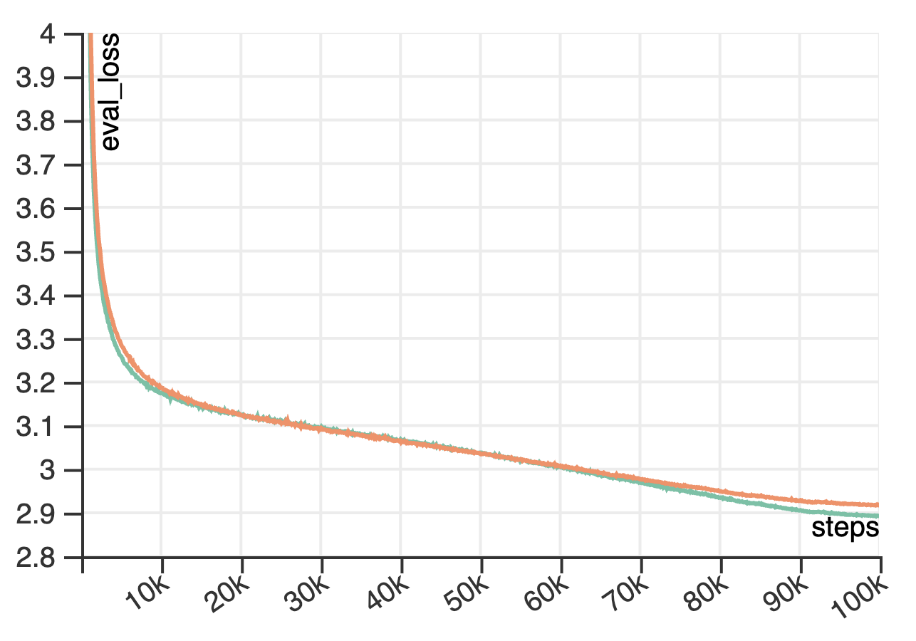
(a) Convergence on miniGPT pretraining

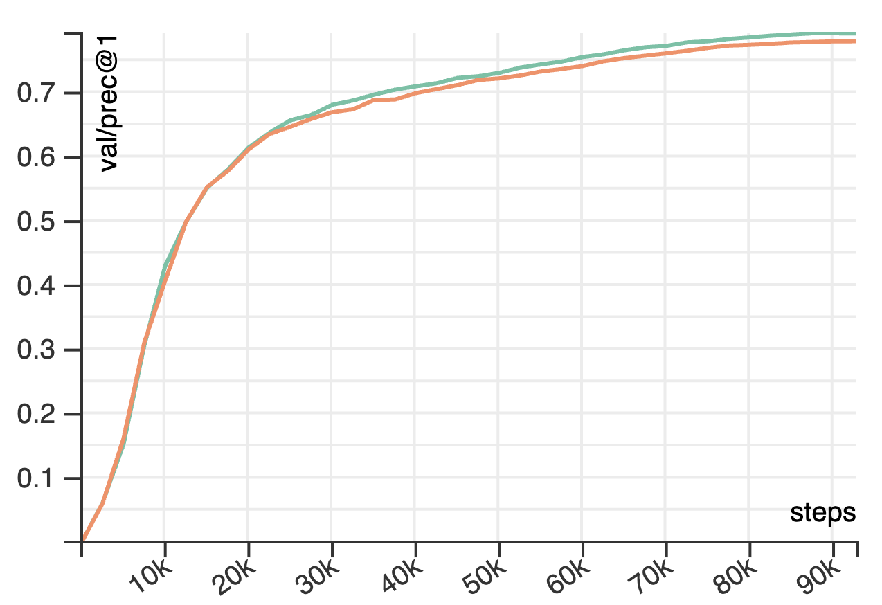
(b) Convergence on Imagenet-1K with VIT

Figure 5: Convergence plots of RGD and Default training regime on real-world datasets. Here the orange line denotes the default training regime, and the green line denotes RGD.

References

- Addepalli et al. (2022) Sravanti Addepalli, Anshul Nasery, R Venkatesh Babu, Praneeth Netrapalli, and Prateek Jain. Learning an invertible output mapping can mitigate simplicity bias in neural networks. arXiv preprint arXiv:2210.01360, 2022.
- Arik & Pfister (2019) Sercan Ömer Arik and Tomas Pfister. Tabnet: Attentive interpretable tabular learning. arxiv. arXiv preprint arXiv:2004.13912, 2019.
- Arjovsky et al. (2019) Martin Arjovsky, Léon Bottou, Ishaan Gulrajani, and David Lopez-Paz. Invariant risk minimization. arXiv preprint arXiv:1907.02893, 2019.
- Arora et al. (2012) Sanjeev Arora, Elad Hazan, and Satyen Kale. The multiplicative weights update method: a meta-algorithm and applications. Theory of computing, 8(1):121–164, 2012.
- Blanchard et al. (2021) Gilles Blanchard, Aniket Anand Deshmukh, Ürun Dogan, Gyemin Lee, and Clayton Scott. Domain generalization by marginal transfer learning. The Journal of Machine Learning Research, 22(1):46–100, 2021.
- Breiman (2001) Leo Breiman. Random forests. Machine learning, 45(1):5–32, 2001.
- Castells et al. (2020) Thibault Castells, Philippe Weinzaepfel, and Jerome Revaud. Superloss: A generic loss for robust curriculum learning. Advances in Neural Information Processing Systems, 33:4308–4319, 2020.
- Cha et al. (2022) Junbum Cha, Kyungjae Lee, Sungrae Park, and Sanghyuk Chun. Domain generalization by mutual-information regularization with pre-trained models. arXiv preprint arXiv:2203.10789, 2022.
- Chawla et al. (2002) Nitesh V Chawla, Kevin W Bowyer, Lawrence O Hall, and W Philip Kegelmeyer. Smote: synthetic minority over-sampling technique. Journal of artificial intelligence research, 16:321–357, 2002.
- Collins et al. (2020) Liam Collins, Aryan Mokhtari, and Sanjay Shakkottai. Task-robust model-agnostic meta-learning. Advances in Neural Information Processing Systems, 33:18860–18871, 2020.
- Cui et al. (2019) Yin Cui, Menglin Jia, Tsung-Yi Lin, Yang Song, and Serge Belongie. Class-balanced loss based on effective number of samples. In Proceedings of the IEEE/CVF conference on computer vision and pattern recognition, pp. 9268–9277, 2019.
- De La Torre & Black (2003) Fernando De La Torre and Michael J Black. A framework for robust subspace learning. International Journal of Computer Vision, 54(1):117–142, 2003.
- Dong et al. (2017) Qi Dong, Shaogang Gong, and Xiatian Zhu. Class rectification hard mining for imbalanced deep learning. In Proceedings of the IEEE International Conference on Computer Vision, pp. 1851–1860, 2017.
- Duchi & Namkoong (2018) John Duchi and Hongseok Namkoong. Learning models with uniform performance via distributionally robust optimization. arXiv preprint arXiv:1810.08750, 2018.
- Duchi et al. (2011) John Duchi, Elad Hazan, and Yoram Singer. Adaptive subgradient methods for online learning and stochastic optimization. Journal of machine learning research, 12(7), 2011.
- Duchi et al. (2021) John C Duchi, Peter W Glynn, and Hongseok Namkoong. Statistics of robust optimization: A generalized empirical likelihood approach. Mathematics of Operations Research, 46(3):946–969, 2021.
- El Hanchi et al. (2022) Ayoub El Hanchi, David Stephens, and Chris Maddison. Stochastic reweighted gradient descent. In International Conference on Machine Learning, pp. 8359–8374. PMLR, 2022.
- Finn et al. (2017) Chelsea Finn, Pieter Abbeel, and Sergey Levine. Model-agnostic meta-learning for fast adaptation of deep networks. In International conference on machine learning, pp. 1126–1135. PMLR, 2017.
- Freund & Schapire (1997) Yoav Freund and Robert E Schapire. A decision-theoretic generalization of on-line learning and an application to boosting. Journal of computer and system sciences, 55(1):119–139, 1997.
- Friedman (2001) Jerome H Friedman. Greedy function approximation: a gradient boosting machine. Annals of statistics, pp. 1189–1232, 2001.
- Ganin et al. (2016) Yaroslav Ganin, Evgeniya Ustinova, Hana Ajakan, Pascal Germain, Hugo Larochelle, François Laviolette, Mario Marchand, and Victor Lempitsky. Domain-adversarial training of neural networks. The journal of machine learning research, 17(1):2096–2030, 2016.
- Gonzalez & Miikkulainen (2021) Santiago Gonzalez and Risto Miikkulainen. Optimizing loss functions through multi-variate taylor polynomial parameterization. In Proceedings of the Genetic and Evolutionary Computation Conference, pp. 305–313, 2021.
- Gulrajani & Lopez-Paz (2020) Ishaan Gulrajani and David Lopez-Paz. In search of lost domain generalization. arXiv preprint arXiv:2007.01434, 2020.
- Hsieh et al. (2019) Ya-Ping Hsieh, Chen Liu, and Volkan Cevher. Finding mixed nash equilibria of generative adversarial networks. In International Conference on Machine Learning, pp. 2810–2819. PMLR, 2019.
- Huang et al. (2020) Zeyi Huang, Haohan Wang, Eric P Xing, and Dong Huang. Self-challenging improves cross-domain generalization. In European Conference on Computer Vision, pp. 124–140. Springer, 2020.
- Jiang et al. (2014a) Lu Jiang, Deyu Meng, Teruko Mitamura, and Alexander G Hauptmann. Easy samples first: Self-paced reranking for zero-example multimedia search. In Proceedings of the 22nd ACM international conference on Multimedia, pp. 547–556, 2014a.
- Jiang et al. (2014b) Lu Jiang, Deyu Meng, Shoou-I Yu, Zhenzhong Lan, Shiguang Shan, and Alexander Hauptmann. Self-paced learning with diversity. Advances in neural information processing systems, 27, 2014b.
- Kahn & Marshall (1953) Herman Kahn and Andy W Marshall. Methods of reducing sample size in monte carlo computations. Journal of the Operations Research Society of America, 1(5):263–278, 1953.
- Katharopoulos & Fleuret (2018) Angelos Katharopoulos and François Fleuret. Not all samples are created equal: Deep learning with importance sampling. In International conference on machine learning, pp. 2525–2534. PMLR, 2018.
- Kingma & Ba (2014) Diederik P Kingma and Jimmy Ba. Adam: A method for stochastic optimization. arXiv preprint arXiv:1412.6980, 2014.
- Krueger et al. (2021) David Krueger, Ethan Caballero, Joern-Henrik Jacobsen, Amy Zhang, Jonathan Binas, Dinghuai Zhang, Remi Le Priol, and Aaron Courville. Out-of-distribution generalization via risk extrapolation (rex). In International Conference on Machine Learning, pp. 5815–5826. PMLR, 2021.
- Kumar et al. (2010) M Kumar, Benjamin Packer, and Daphne Koller. Self-paced learning for latent variable models. Advances in neural information processing systems, 23, 2010.
- Kumar et al. (2022) Ramnath Kumar, Tristan Deleu, and Yoshua Bengio. The effect of diversity in meta-learning. arXiv preprint arXiv:2201.11775, 2022.
- Lam (2016) Henry Lam. Robust sensitivity analysis for stochastic systems. Mathematics of Operations Research, 41(4):1248–1275, 2016.
- Lam (2019) Henry Lam. Recovering best statistical guarantees via the empirical divergence-based distributionally robust optimization. Operations Research, 67(4):1090–1105, 2019.
- Le et al. (2011) Quoc V Le, Jiquan Ngiam, Adam Coates, Abhik Lahiri, Bobby Prochnow, and Andrew Y Ng. On optimization methods for deep learning. In Proceedings of the 28th international conference on international conference on machine learning, pp. 265–272, 2011.
- Leng et al. (2022) Zhaoqi Leng, Mingxing Tan, Chenxi Liu, Ekin Dogus Cubuk, Xiaojie Shi, Shuyang Cheng, and Dragomir Anguelov. Polyloss: A polynomial expansion perspective of classification loss functions. arXiv preprint arXiv:2204.12511, 2022.
- Li et al. (2018a) Da Li, Yongxin Yang, Yi-Zhe Song, and Timothy Hospedales. Learning to generalize: Meta-learning for domain generalization. In Proceedings of the AAAI conference on artificial intelligence, volume 32, 2018a.
- Li et al. (2018b) Haoliang Li, Sinno Jialin Pan, Shiqi Wang, and Alex C Kot. Domain generalization with adversarial feature learning. In Proceedings of the IEEE conference on computer vision and pattern recognition, pp. 5400–5409, 2018b.
- Li et al. (2018c) Ya Li, Xinmei Tian, Mingming Gong, Yajing Liu, Tongliang Liu, Kun Zhang, and Dacheng Tao. Deep domain generalization via conditional invariant adversarial networks. In Proceedings of the European Conference on Computer Vision (ECCV), pp. 624–639, 2018c.
- Lin et al. (2017) Tsung-Yi Lin, Priya Goyal, Ross Girshick, Kaiming He, and Piotr Dollár. Focal loss for dense object detection. In Proceedings of the IEEE international conference on computer vision, pp. 2980–2988, 2017.
- Majmundar et al. (2022) Kushal Majmundar, Sachin Goyal, Praneeth Netrapalli, and Prateek Jain. Met: Masked encoding for tabular data. arXiv preprint arXiv:2206.08564, 2022.
- Nam et al. (2021) Hyeonseob Nam, HyunJae Lee, Jongchan Park, Wonjun Yoon, and Donggeun Yoo. Reducing domain gap by reducing style bias. In Proceedings of the IEEE/CVF Conference on Computer Vision and Pattern Recognition, pp. 8690–8699, 2021.
- Namkoong & Duchi (2017) Hongseok Namkoong and John C Duchi. Variance-based regularization with convex objectives. Advances in neural information processing systems, 30, 2017.
- Nemirovsky et al. (1983) AS Nemirovsky, DB Yudin, and ER DAWSON. Wiley-interscience series in discrete mathematics, 1983.
- Rahimi & Recht (2008) Ali Rahimi and Benjamin Recht. Weighted sums of random kitchen sinks: Replacing minimization with randomization in learning. Advances in neural information processing systems, 21, 2008.
- Ren et al. (2018) Mengye Ren, Wenyuan Zeng, Bin Yang, and Raquel Urtasun. Learning to reweight examples for robust deep learning. In International conference on machine learning, pp. 4334–4343. PMLR, 2018.
- Requeima et al. (2019) James Requeima, Jonathan Gordon, John Bronskill, Sebastian Nowozin, and Richard E Turner. Fast and flexible multi-task classification using conditional neural adaptive processes. Advances in Neural Information Processing Systems, 32, 2019.
- Ruder (2016) Sebastian Ruder. An overview of gradient descent optimization algorithms. arXiv preprint arXiv:1609.04747, 2016.
- Sagawa et al. (2019) Shiori Sagawa, Pang Wei Koh, Tatsunori B Hashimoto, and Percy Liang. Distributionally robust neural networks for group shifts: On the importance of regularization for worst-case generalization. arXiv preprint arXiv:1911.08731, 2019.
- Shamir & Zhang (2013) Ohad Shamir and Tong Zhang. Stochastic gradient descent for non-smooth optimization: Convergence results and optimal averaging schemes. In International conference on machine learning, pp. 71–79. PMLR, 2013.
- Shu et al. (2019) Jun Shu, Qi Xie, Lixuan Yi, Qian Zhao, Sanping Zhou, Zongben Xu, and Deyu Meng. Meta-weight-net: Learning an explicit mapping for sample weighting. Advances in neural information processing systems, 32, 2019.
- Sinha et al. (2017) Aman Sinha, Hongseok Namkoong, Riccardo Volpi, and John Duchi. Certifying some distributional robustness with principled adversarial training. arXiv preprint arXiv:1710.10571, 2017.
- Snell et al. (2017) Jake Snell, Kevin Swersky, and Richard Zemel. Prototypical networks for few-shot learning. Advances in neural information processing systems, 30, 2017.
- Sun & Saenko (2016) Baochen Sun and Kate Saenko. Deep coral: Correlation alignment for deep domain adaptation. In European conference on computer vision, pp. 443–450. Springer, 2016.
- Ucar et al. (2021) Talip Ucar, Ehsan Hajiramezanali, and Lindsay Edwards. Subtab: Subsetting features of tabular data for self-supervised representation learning. Advances in Neural Information Processing Systems, 34:18853–18865, 2021.
- Vapnik (1999) Vladimir N Vapnik. An overview of statistical learning theory. IEEE transactions on neural networks, 10(5):988–999, 1999.
- Verma et al. (2021) Vikas Verma, Thang Luong, Kenji Kawaguchi, Hieu Pham, and Quoc Le. Towards domain-agnostic contrastive learning. In International Conference on Machine Learning, pp. 10530–10541. PMLR, 2021.
- Wainwright (2019) Martin J Wainwright. High-dimensional statistics: A non-asymptotic viewpoint, volume 48. Cambridge university press, 2019.
- Wang et al. (2017) Yixin Wang, Alp Kucukelbir, and David M Blei. Robust probabilistic modeling with bayesian data reweighting. In International Conference on Machine Learning, pp. 3646–3655. PMLR, 2017.
- Yan et al. (2020) Shen Yan, Huan Song, Nanxiang Li, Lincan Zou, and Liu Ren. Improve unsupervised domain adaptation with mixup training. arXiv preprint arXiv:2001.00677, 2020.
- Yoon et al. (2020) Jinsung Yoon, Yao Zhang, James Jordon, and Mihaela van der Schaar. Vime: Extending the success of self-and semi-supervised learning to tabular domain. Advances in Neural Information Processing Systems, 33:11033–11043, 2020.
- Zadrozny (2004) Bianca Zadrozny. Learning and evaluating classifiers under sample selection bias. In Proceedings of the twenty-first international conference on Machine learning, pp. 114, 2004.
- Zeiler (2012) Matthew D Zeiler. Adadelta: an adaptive learning rate method. arXiv preprint arXiv:1212.5701, 2012.
- Zhai et al. (2021) Runtian Zhai, Chen Dan, Arun Suggala, J Zico Kolter, and Pradeep Ravikumar. Boosted cvar classification. Advances in Neural Information Processing Systems, 34:21860–21871, 2021.
- Zhang et al. (2021) Marvin Zhang, Henrik Marklund, Nikita Dhawan, Abhishek Gupta, Sergey Levine, and Chelsea Finn. Adaptive risk minimization: Learning to adapt to domain shift. Advances in Neural Information Processing Systems, 34:23664–23678, 2021.
- Zhang & Pfister (2021) Zizhao Zhang and Tomas Pfister. Learning fast sample re-weighting without reward data. In Proceedings of the IEEE/CVF International Conference on Computer Vision, pp. 725–734, 2021.
- Zhu et al. (2023) Deyao Zhu, Jun Chen, Xiaoqian Shen, Xiang Li, and Mohamed Elhoseiny. Minigpt-4: Enhancing vision-language understanding with advanced large language models. arXiv preprint arXiv:2304.10592, 2023.
- (69) Lanyun Zhu, Tianrun Chen, Jianxiong Yin, Simon See, and Jun Liu. Reinforced sample reweighting policy for semi-supervised learning.
- Zhu et al. (2015) Yukun Zhu, Ryan Kiros, Rich Zemel, Ruslan Salakhutdinov, Raquel Urtasun, Antonio Torralba, and Sanja Fidler. Aligning books and movies: Towards story-like visual explanations by watching movies and reading books. In Proceedings of the IEEE international conference on computer vision, pp. 19–27, 2015.