Survival of the flattest in the quasispecies model
Abstract
Viruses present an amazing genetic variability. An ensemble of infecting viruses, also called a viral quasispecies, is a cloud of mutants centered around a specific genotype. The simplest model of evolution, whose equilibrium state is described by the quasispecies equation, is the Moran–Kingman model. For the sharp peak landscape, we perform several exact computations and we derive several exact formulas. We obtain also an exact formula for the quasispecies distribution, involving a series and the mean fitness. A very simple formula for the mean Hamming distance is derived, which is exact and which do not require a specific asymptotic expansion (like sending the length of the macromolecules to or the mutation probability to ). We try also to extend these formulas to a general fitness landscape. We obtain an equation involving the covariance of the fitness and the Hamming class number in the quasispecies distribution. With the help of these formulas, we discuss the phenomenon of the error threshold and the notion of quasispecies. We recover the limiting quasipecies distribution in the long chain regime. We go beyond the sharp peak landscape and we consider fitness landscapes having finitely many peaks and a plateau–type landscape. We finally prove rigorously within this framework the possible occurrence of the survival of the flattest, a phenomenon which has been previously discovered by Wilke, Wang, Ofria, Lenski and Adami [21] and which has been investigated in several works [6, 14, 19, 20].
1 Introduction
Viruses are very hard to fight because of their genetic diversity. They mutate constantly in order to escape the attacks of the immune system of their host. At the same time, the genotypes of an infecting population of viruses are strongly correlated, they look like a cloud of mutants centered around a specific genotype. This population structure, called a quasispecies, can be observed experimentally for viruses (in vivo studies have been conducted for the HIV [17] and the hepatitis C virus [12]). Nowadays, deep sequencing techniques allow to collect data on the structure of viral quasispecies. Yet the various biological mechanisms involved in the creation and the evolution of quasispecies are far from being understood (see [9] for a recent review or the book [8] for a more comprehensive account). In order to develop efficient antiviral therapies, it is crucial to design simple mathematical models of quasispecies. In principle, a quasispecies can occur in any biological population whose evolution is driven by mutation and selection. We shall first present a very simple model for the evolution of a population under mutation and selection. We write then the equations describing the equilibrium of this model, thereby recovering directly the quasispecies equation associated to the equilibrium of Eigen’s model. The model is precisely defined in section 2, but let us introduce it briefly on the binary space in order to state some of our main results (the general versions are kept further in the text).
Genotypes. The genotypes are binary sequences of length .
Mutations. The mutations happen independently at each site of the sequence, with probability .
Sharp peak landscape. The fitness function is a sharp peak: there is a privileged genotype, , referred to as the master sequence, which has a higher fitness than the rest. Let and let the fitness function be given by
In the simplified framework of the sharp peak landscape, we perform several exact computations and we derive several exact formulas. In particular, we obtain a remarkable equation for the mean fitness at equilibrium, which had been previously discovered by Bratus, Novozhilov and Semenov, see formulas and in [3]. We state next a probabilistic version of this formula. Let be a random variable with distribution the binomial law with parameters and . Denoting by the expectation, the mean fitness at equilibrium satisfies
| (1.1) |
Bratus, Novozhilov and Semenov exploited this equation to derive rigorous bounds on the mean fitness, but this formula has wider applications. Furthermore, we obtain also in section 6 an exact formula for the quasispecies distribution, involving a series and the mean fitness. A very simple formula for the mean Hamming distance is derived, which is exact and which do not require a specific asymptotic expansion, like sending the length of the macromolecules to or the mutation probability to . The mean Hamming distance in the quasispecies distribution can be interpreted as the mean number of ones in a genotype at equilibrium, and the formula is
where is the mean fitness of the population. We try also to extend these formulas to a general fitness landscape in sections 7, 8. In theorem 9.11, we obtain an equation involving the covariance of the fitness and the Hamming class number in the quasispecies distribution. These formulas shed new insight into the classical phenomenon of the error threshold and the notion of quasispecies, which are discussed in section 11. We consider the asymptotic regime, called the long chain regime, where
The parameter is in fact the mean number of observed mutations per individual in each reproduction cycle. We denote by the mean fitness at equilibrium and by the proportion of the wild type in the population at equilibrium.
Theorem 1.2 (Error threshold).
For the sharp peak landscape, we have the following dichotomy:
If , then , whence .
If , then , and
Thus the limit of the proportion of the wild type present in the population is positive only if , or equivalently, if asymptotically . The value
is the error threshold, described by Eigen as the critical mutation rate above which the wild type disappears from the population. In section 11, we discuss further the relevance of this classical result and we show how the well–known theorem 1.2 follows easily from equation (1.1). With the help of the exact formulas derived in section 6, we recover the limiting quasipecies distribution in the long chain regime in section 12.
Most of the rigorous mathematical analysis of Eigen’s model deals with the sharp peak landscape, or with landscapes presenting a lot of symmetries (see [2] for the analysis of a permutation invariant fitness landscape and [4] for a review of the literature). We go beyond the sharp peak landscape and we consider fitness landscapes having finitely many peaks in section 13.
Finitely many peaks. We suppose that there exist a fixed integer and fixed values such that: for any value of , there exist peaks in (whose localization may vary with and ) such that the fitness function is given by
We shall prove the following theorem.
Theorem 1.3 (Error threshold for finitely many peaks).
Let us set
Let be the mean fitness for the model associated to the fitness function and the parameters . We have the following dichotomy:
If , then .
If , then .
We see that the situation is very similar to the case of the sharp peak landscape. The critical parameter depends now on the fitness of the highest peak. The conclusion is that a finite number of peaks do not really interfere with each other, and their respective contributions to the global equilibrium of the model are essentially independent. In section 14, we consider the case of a Plateau and we derive an equation satisfied by the mean fitness at equilibrium.
Survival of the flattest. In section 15, we finally prove rigorously within this framework the possible occurrence of the survival of the flattest, a phenomenon which has been previously discovered by Wilke, Wang, Ofria, Lenski and Adami [21] and which has been investigated in several works [6, 14, 19, 20]. We state next the precise mathematical result we obtain. Let and let be the fitness function given by
Theorem 1.4.
Let and let be the unique real number such that
Let be the mean fitness for the model associated to the fitness function and the parameters . We have the following convergence in the long chain regime:
Let us denote by the fraction of the sequence in the population at equilibrium, and by the fraction of the sequences having zeroes and and ones in the population at equilibrium.
If , then , .
If , then , .
We show finally that we can find adjust the values and in such a way that and . For such values, the quasispecies will be located on the plateau, despite the fact that the height of the plateau is strictly less than the height of the peak. In this situation, we witness the survival of the flattest. The road to prove theorems 1.3 and 1.4 is quite long. It rests on the exact formulas proved in section 8 and a general strategy developed in section 7.
2 The quasispecies equations
We consider a population of haploid individuals evolving under the conjugate effects of mutation and selection. We suppose that the population has reached an equilibrium around a specific well adapted individual, called the wild type, and denoted by . Individuals reproduce, yet the reproduction mechanism is error–prone, and mutations occur constantly. These mutations drive the genotypes away from . Yet has a selective advantage because it reproduces faster.
We would like to characterize mathematically this kind of equilibrium. We denote by the set of the possible genotypes, which we assume to be finite. Generic elements of are denoted by the letters . The Darwinian fitness of an individual having genotype is denoted by , it can be thought of as its mean number of offspring. In addition, mutations occur in each reproduction cycle, an individual of type might appear as the result of mutations from offspring of other types. Let us denote by the probability that the offspring of an individual of type is of type . Of course, we have
We introduce next the linear model, one of the simplest models for the evolution of a population with selection and mutation. We suppose that the successive generations do not overlap and we denote by the number of individuals of type in the generation . The linear model assumes that an individual of type produces offspring at a rate proportional to its fitness , and that a proportion of the offspring mutates and becomes of type , thus is given by the formula
The trouble with this formula is that the sum is not necessarily an integer. To go around this problem, a natural way is to develop stochastic population models, in such a way that the above formula describes the evolution of the mean number of individuals. The archetype of this kind of models is the Galton–Watson branching process. If we introduce in addition a constraint on the total size of the population, then we would consider the classical Wright–Fisher model. Yet the randomness adds an extra layer of complexity and stochastic models are considerably harder to study. Another simpler possibility is to consider the proportions of each type of individuals in the population, instead of their numbers, as Moran and Kingman did in the late seventies [16, 18]. Let us denote by the proportion of individuals of type in the generation . The model proposed by Moran is given by
The denominator has been chosen to ensure that . In fact, this model consists in iterating a deterministic map on the function encoding the proportions of each type present in the population. The possible equilibria of the model correspond to the fixed points of this map, that is the solutions of the following equations:
| (2.1) |
subject to the constraint
| (2.2) |
We call these equations the quasispecies equations. They characterize also the equilibrium in the model originally developed by Eigen [10], which led to the quasispecies theory.
3 The sharp peak landscape
Ideally, we would like to have explicit formulas for in terms of and . Unfortunately, there is little hope of obtaining such explicit formulas in the general case. So we consider the simplest non neutral fitness function which comes to mind, the sharp peak fitness function: there is a privileged genotype, , referred to as the master sequence, which has a higher fitness than the rest. Let and let the fitness function be given by
| (3.1) |
This is the fitness function that Eigen studied in detail in his article [10]. Despite its apparent simplicity, this model leads to interesting mathematical questions and it provides new insight into the genetic structure of a population. Eigen and Schuster [11] discussed the sharp peak landscape (which is fully presented in section 4) with the help of approximation techniques and in a specific asymptotic regime. We present here a new approach, which is more elementary. In fact, we shall compute exact formulas for the solution.
Suppose that is a solution of the system (2.1) satisfying the constraint (2.2). Let be the mean fitness of this solution, defined by
| (3.2) |
Obviously, the mean fitness satisfies and if and only if . Moreover all the coefficients of the mutation matrix are positive, and it follows from equation (2.1) that
| (3.3) |
Therefore for all . The equation (2.1) for a generic genotype reads:
| (3.4) |
We rewrite this equation as
| (3.5) |
Using this very formula for , we replace in the sum, thereby getting
We iterate this process. After steps, we get
The sums of products involving the matrix have a natural probabilistic interpretation. Let be the Markov chain on with transition matrix . The previous formula for can now be rewritten as
By (3.2) and (3.3), the mean fitness is strictly larger than one, therefore the last term goes to as goes to . Sending to , and using the fact that
| (3.6) |
we get the following result.
Proposition 3.7.
Let us take in formula (3.8). Using again (3.6), we obtain
| (3.9) |
The right-hand side of this equation is a continuous decreasing function of , which is equal to when and is less or equal than when . Therefore there exists exactly one value of in which satisfies this equation. Our next goal is to obtain an explicit expression for and to perform the summation of the series appearing in (3.9). To do so, we shall make additional assumptions on the geometry of the fitness landscape.
4 Mutation dynamics
From now onwards, we focus on a particular choice of the set of genotypes and of the mutation matrix . Both for practical and historical reasons, we make the same choice as Eigen and Schuster [11], which leads to the sharp peak landscape.
Genotypes. We consider the different genotypes to be sequences of length over an alphabet of cardinality . Standard examples are , , for binary sequences or , , to model DNA molecules. The –th component of a genotype is denoted by . The Hamming distance counts the number of differences between two sequences:
Mutations. We suppose that mutations happen independently along the sequence, with probability . For , the mutation probability is given by
| (4.1) |
The previous choices for the set of the genotypes and for the mutation mechanism, together with the fitness function (3.1), determine the sharp peak landscape. In this model, the mutations occur independently at each site. An important consequence of this structural assumption is that the components of the Markov chain are themselves independent Markov chains with state space and transition matrix
The non-diagonal terms in this matrix are all equal to . Since we want to compute , we shall lump together the letters which differ from the wild type , and we shall do this for each component. More precisely, we define a process by setting
The binary word indicates the sites where and differ. In particular, is a deterministic function of . Thanks to the specific form of the transition matrix, it turns out that is still a Markov chain. This is a particular case of the lumping theorem of Kemeny and Snell [15]. To see why it is so, let us consider for instance the first two steps of the first component and let us compute
The simplification in the final result comes from the fact that the probabilities to find or to lose a letter from the wild type are the same for all the letters in . A similar computation can be done for a finite number of steps. We conclude that is the two states Markov chain that we define and study next. Let be the Markov chain with state space and transition matrix
The eigenvalues of are and
| (4.2) |
It is a standard exercise to compute the powers of :
Here is a simple illuminating way to realize the Markov chain and to understand the expression of the –th power . Let be an i.i.d. sequence of Bernoulli random variables with parameter . Suppose that . If , then we set . If , then we choose a letter uniformly over , independently of the past history until time , and we set if the chosen letter is the one of the wild type and otherwise. Now, the event can occur in two different ways. Either , or one of the is zero, in which case with probability and with probability , thus
and we recover the expression of the diagonal coefficients of . In words, the status at step is the same than at time if no mutation has occurred, or if the last mutation yields the same letter than the wild type (case ) or a different letter (case ). Similarly, the event can occur only if one of the is zero, and the last mutation event yields the adequate letter, thus
Now the probability can be rewritten with the help of and as
| (4.3) |
5 The equation for the mean fitness
Substituting the expression obtained in (4.3) into formula (3.9), we obtain
| (5.1) |
We expand the power in , we exchange the summations and we re-sum the series as follows:
Thus the equation satisfied by the mean fitness reads:
| (5.2) |
This equation was discovered by Bratus, Novozhilov and Semenov, see formulas and in [3], they exploited this equation to derive rigorous bounds on the mean fitness. This formula calls naturally for a probabilistic interpretation. Let be a random variable with distribution the binomial law with parameters and . Denoting by the expectation, equation (5.2) can be rewritten as
| (5.3) |
Our analysis of the quasispecies equations on the sharp peak landscape rests on the identity (5.1) or its equivalent form (5.3). Indeed, if we manage to estimate the mean fitness , then we will also have an estimate on the proportion of the wild type present in the population. Moreover, once we know or , the proportions of the other types are completely determined by formula (3.8).
6 An exact formula for the quasispecies
Loosely speaking, a quasispecies is a cloud of mutants centered around a specific genotype. The structure of this cloud depends on the parameters and . In fact, the proportion of the wild type decreases as the mutation rate increases, and it becomes comparable to the proportions of the other genotypes when reaches the error threshold . This fascinating phenomenon will be proved rigorously in section 11. When is a little below , we observe a cloud of mutants centered around which contains a very small proportion of the wild type , the vast majority of the genotypes present in the population will differ from . Yet the genetic information carried out by is still present in the population and it determines its structure. This paradoxical situation has led several biologists to argue that the selection operates at the level of the quasispecies, and not at the level of individuals [9]. Thus an important goal is to understand better the statistical composition of the cloud of mutants. In order to do so, we classify the genotypes according to their Hamming distance to the wild type . For , we define the Hamming class as the set of the genotypes which differ from at exactly indices, i.e.,
| (6.1) |
We shall exploit further formula (3.8) in order to derive an exact formula for the proportion of the genotypes belonging to the Hamming class . For , we have, thanks to formula (3.8),
| (6.2) |
We have already noticed that the components of , , are independent Markov chains. Therefore, using the notation of section 4,
| (6.3) |
Recall that . Plugging (6.3) in (6.2), we get an exact formula for the quasispecies distribution, in terms of a series involving and :
| (6.4) |
We can even compute the sum of the series, by developing the powers, and we get a finite algebraic formula:
| (6.5) |
Of course this formula is complicated, yet it expresses completely the dependence of as a function of and and it shows the complexity of the sharp peak landscape. Surprisingly, the mean and the variance of the Hamming distance of the quasispecies distribution have very simple expressions. Indeed, the mean of the Hamming distance of the distribution is given by
| (6.6) |
To compute this mean, we rely on formula (6.4) to write
| (6.7) |
In the inner sum, we recognize the expectation of a binomial law, whence
By summing the geometric series and using the definition of , we obtain formula (6.6). In fact, all the successive moments of the quasispecies distribution can be computed in this way.
7 Extension to a general landscape
We try here to extend the formulas obtained in section 3 to a general fitness landscape. We still use the same genotype space and the same mutation kernel as for the sharp peak landscape and we make the following hypothesis on the fitness function .
Hypothesis 7.1.
The fitness function is larger or equal than , and it is not identically equal to .
Our starting point is the quasispecies equation (2.1), rewritten in the following form:
| (7.2) |
subject to the constraint
| (7.3) |
where
is the mean fitness, or equivalently the Perron–Frobenius eigenvalue of the matrix . Thanks to the hypothesis on the fitness function, we have that . Moreover, since the matrix has only positive entries and since the fitness function is not identically equal to , then the Perron–Frobenius eigenvalue is in fact strictly larger than one, i.e., . We rewrite the equation (7.2) as
| (7.4) |
We denote by the line vector which is the transpose of the column vector and we introduce the square matrix whose diagonal coefficients are the fitness values :
| (7.5) |
After dividing by (recall that ), equation (7.4) can be rewritten in matrix form as
| (7.6) |
Now the matrix is a stochastic matrix, hence its spectral radius is equal to . Since , then the matrix is invertible, and its inverse is given by the geometric series:
Plugging this identity into equation (7.6), we obtain
| (7.7) |
Let us introduce the set of the genotypes where the fitness function is strictly larger than one:
We call the set the set of the wildtypes. We introduce the matrix , indexed by the elements of , defined as
| (7.8) |
With these notations, the linear system (7.7) of size can be split into the system of size given by
| (7.9) |
and the remaining equations
| (7.10) |
The system (7.9) expresses that the vector is a Perron–Frobenius eigenvector of the matrix , and that the Perron–Frobenius eigenvalue of is equal to . The equations (7.10) show that the remaining coordinates are completely determined by . These considerations suggest that the quasispecies equation can in principle be solved through the following procedure.
General strategy. We start by isolating the set of the wild types and we form the matrix , defined in formula (7.8), where is considered as a parameter. Now, the Perron–Frobenius eigenvalue of is a decreasing function of , which tends to as goes to and to as goes to . We choose for the unique value such that the Perron–Frobenius eigenvalue of is equal to . Once this value is fixed, we solve the system (7.9) on . The remaining coordinates of on are determined by equations (7.10).
A general lower bound on . We close this section with a general lower bound on . The quasispecies equations imply that
Since for any , this readily implies that
| (7.11) |
8 Computation of
We start by computing . We use the notations and the technique of section 4 and we generalize formula (4.3) as follows:
| (8.1) |
Now, we have
| (8.2) |
where
Coming back to formula (8.1), we conclude that
| (8.3) |
We wish now to compute
Our first strategy consists in developing formula (8.3), we end up with several geometric series and we obtain a closed finite formula. So, starting from (8.3), we have, setting to alleviate the notation,
| (8.4) |
We can now sum up the series and we get
| (8.5) |
We provide furthermore a probabilistic interpretation of this apparently complex formula. Let be a binomial random variable with parameters . We have
| (8.6) |
The above formula is quite nice, its drawback is that it contains negative terms, so it is not obvious to see that the global result is non-negative. We present next a third formula, which avoids this problem. The trick consists in developing the factor of formula (8.3) in a more complicated way, as follows:
| (8.7) |
We wish to compute the series . From now onwards, we deal with the case (for , we use the expression obtained in (8.5), where all the terms are positive). After extracting the two terms which depend on , we end up with the series
| (8.8) |
Notice that this formula is not quite legitimate for , unless we make the convention that, for , there is only one term in the sum corresponding to . Therefore it seems safer to perform the above computation only when . Let us set and let us focus on the sum
| (8.9) |
We shall decompose the sum according to the number of distinct indices among , their different values , and the number of times each value appear. We get
| (8.10) |
The number of terms appearing in the last summation corresponds to the number of placements of balls in cells with occupancy numbers given by (see for instance the classical book of Feller [13], section II.5), that is . For each of these placements, we have
therefore the formula (8.10) becomes
| (8.11) |
We can perform the summation over , and we get
| (8.12) |
The number of indices has decreased by , and has been replaced by . We proceed in the same way and we perform successively the summations over until we obtain
Recalling that , we can compute the last sum
and we conclude that
| (8.13) |
Putting together formulas (8.10), (8.11), (8.12), (8.13), we obtain a finite formula for the sum (8.9):
| (8.14) |
Plugging this formula into (8.8) and (8.7) yields that, for ,
| (8.15) |
We can further rewrite this formula using the expectation with respect to a Binomial random variable with parameters and . Indeed, we have
| (8.16) |
Each of the previous formulas has its own interest and might be useful, depending on the context. For instance, with formula (8.5), we see directly that the coefficients of the matrix are rational functions of the parameter , and that there exists a unique choice for such that the Perron–Frobenius eigenvalue of becomes equal to . The analysis of the error threshold conducted in section 11 rests entirely on the probabilistic representation presented in formula (8.6) in the specific case where and . Finally, the third formula (8.16) will be useful to analyze the asymptotic behavior of the non-diagonal entries of the matrix for the landscape with finitely many peaks in section 13.
9 A curious formula
Throughout this section, we denote by the alphabet over which is built, so that and . Let be an additive functional, that is a function given by
where is a function defined on with values in . We consider an arbitrary fitness function satisfying the hypothesis 7.1, and we denote by , the solution of the quasispecies equation associated to . Our goal here is to relate the mean value of in the quasispecies , defined by
to the mean fitness or , defined by
Our starting point is formula (7.7), which yields
| (9.1) | ||||
| (9.2) |
We compute next the most inner sum. By the definition of ,
| (9.3) |
Moreover, formulas (8.1) and (8.2) yield that, for ,
| (9.4) |
where is the mean value of over the alphabet , i.e.,
| (9.5) |
Plugging formula (9.4) in formula (9.3), we obtain
| (9.6) |
Inserting this last formula into (9.1), we obtain
| (9.7) | ||||
| (9.8) | ||||
| (9.9) |
where we have introduced the notation
| (9.10) |
Recalling that , we have proved the curious formula stated in the next theorem.
Theorem 9.11.
Let be a finite alphabet of cardinality and let . Let be a function defined on with values in and let be defined by
For any fitness function over the genotype set , which is larger or equal than , and which is not identically equal to , we have
| (9.12) |
where is defined above in (9.10), is given in (4.2) and
Let us look at the specific case of the sharp peak landscape studied in section 4. We take , , and the fitness function defined in formula (3.1). For the function , we take the identity function on , so that, for any , the value is simply the Hamming class of . In particular, we have and , so that the formula (9.12) becomes
| (9.13) |
which is precisely the formula (6.6) that we obtained previously in this context. We can also consider the neutral case. If the fitness function is constant, then the quasispecies distribution is in fact the uniform distribution over the genotype space, so that , and the above relation (9.13) still holds. This is not too surprising, because it amounts to the case where the fitness of the wildtype is equal to .
10 Sharp peak landscape: an upper bound on
We consider here the case of the sharp peak landscape described in section 3. In order to get an upper bound on , we start from the identity (5.3). From the weak law of large numbers, we know that the most likely values for are those around its mean , so we pick a positive number and we split the expectation as follows:
| (10.1) | ||||
| (10.2) |
Taking advantage from the fact that , we bound by in the first sum and by in the second, this leads to the inequality
| (10.3) |
We apply the Chebyshev inequality to the binomial random variable and we get the classical estimate:
| (10.4) |
Plugging the Chebyshev inequality into (10.3), we conclude that
| (10.5) |
Let us pause for one moment to look at this inequality. Obviously, as goes to , the right-hand side goes to , and the inequality cannot hold. In other words, for this inequality to hold, must not be too large. Thus, from this inequality, we should be able to derive an upper bound on . To get the best possible upper bound, we could rewrite it as a polynomial inequality of degree two in and compute the associated roots, but this leads to messy expressions. Instead, after a few trials (hidden to the reader), we obtain the following inequality.
Lemma 10.6.
The mean fitness satisfies
| (10.7) |
Proof.
Suppose that is larger than the upper bound in (10.7). We check that this is not compatible with inequality (10.5) with the choice . Indeed, we have on one hand
On the other hand,
Applying the mean value theorem to the function on the interval , we have
| (10.8) |
Combining the previous inequalities, we obtain that
which stands in contradiction with the inequality (10.5) with . ∎
11 The error threshold
We are now in position to demonstrate that the quasispecies equation undergoes a phenomenon similar to a phase transition. We consider the asymptotic regime, called the long chain regime, where
| (11.1) |
and we shall discuss the behavior of the system according to the parameter . The parameter is in fact the mean number of observed mutations per individual in each reproduction cycle.
Theorem 11.2 (Error threshold).
We have the following dichotomy:
If , then , whence .
If , then , and
| (11.3) |
Thus the limit of the proportion of the wild type present in the population is positive only if , or equivalently, if asymptotically . The value
is the error threshold, described by Eigen as the critical mutation rate above which the wild type disappears from the population. In the absence of mutations, that is for , we have and the only genotype present in the population is the wild type . In the presence of a small amount of mutations, that is for , genetic diversity is constantly reintroduced in the population and there is a positive proportion of the genotypes which differ from . Yet most of the genotypes are very close to the wild type . In fact, the population looks like a cloud of mutants centered around the wild type. As the mutation rate is raised, the proportion of the wild type present in the population decreases. When reaches the error threshold, the wild type disappears from the population, more precisely the proportion of the wild type becomes comparable to the proportions of the other genotypes. This is the error catastrophe: the selective advantage of the wild type is annihilated by the mutations.
This kind of equilibrium was discovered within the framework of Eigen’s model and was called a quasispecies [10, 11], as opposed to a species, which refers to an homogeneous solution in chemistry. In fact, Eigen’s model is a model for the evolution of a population of macromolecules governed by a system of chemical reactions and the laws of kinetics yield a differential system of equations whose equilibrium is described by the quasispecies equation. This system was historically analyzed with approximation and expansion techniques, which in the asymptotic regime (11.1) led to the discovery of the error threshold.
Although the original goal of Eigen was to understand the first stages of life on Earth, the notion of quasispecies and the error threshold had a profound impact on the understanding of molecular evolution [9]. Indeed, many living organisms seem to satisfy approximately the scaling relation
Unfortunately, for complex creatures, it is very complicated to estimate the mutation rate, which is usually extremely small. Viruses, however, have a rather high mutation rate, and the orders of magnitude of their genome length and their mutation rate is compatible with this scaling law. Moreover, some RNA viruses, like the HIV virus, evolve with a high mutation rate which seems to be close to an error threshold [9]. Why is that so?
In order to survive a virus should achieve two goals. First, its genetic information should be preserved from one generation to another, hence its mutation rate has to be below the error threshold. Second, it has to escape the attacks of the immune system of its hosts, and to do so, it should mutate as fast as possible. The most efficient strategy is therefore to adjust the mutation rate to the left of the error threshold: this will achieve simultaneously a huge genetic variability, and the preservation of the pertinent genetic information across generations. Some promising antiviral strategies, called lethal mutagenesis, consist in using mutagenic drugs which increase slightly the mutation rate of the virus in order to induce an error catastrophe [1, 7, 9].
Because of its importance, we shall give two proofs of theorem 11.2. The first proof is a soft proof based on a compactness argument, whose starting point is the initial quasispecies equation. The second proof is a more technical proof, whose starting point is the equation (5.1) discovered by Bratus, Novozhilov and Semenov. Naturally, the second proof is more informative, it yields a control on the speed of convergence and it opens the way to perform an asymptotic expansion of with respect to and .
From equation (3.2), we can express as
| (11.4) |
Therefore it is enough to study the asymptotic behavior of . We shall prove that
| (11.5) |
Soft proof.
In the long chain regime, we have
| (11.6) |
Using the lower bound (7.11) and the fact that , we see that
| (11.7) |
Suppose that does not converge towards . In this case, there exist and two sequences of parameters , such that
| (11.8) |
Using (11.4) and (11.8), we obtain a lower bound on :
| (11.9) |
We bound from above the quasispecies equation (2.1) associated to , as follows:
| (11.10) | ||||
| (11.11) |
where we have used the fact that whenever . Using together (11.9) and (11.10), we obtain that
Sending to , we see that this inequality is not coherent with inequality (11.8). Therefore it must be the case that converges towards . ∎
Technical proof.
This proof is entirely based on the equation (5.1) discovered by Bratus, Novozhilov and Semenov, see formulas and in [3], and its probabilistic interpretation (5.3). Let us start with a simple interesting inequality on . The map
is convex. The equation (5.1) (or rather (5.3)) can be rewritten with the help of the function as
| (11.12) |
where is a random variable with distribution the binomial law with parameters and . By the classical Jensen inequality, we have therefore
| (11.13) |
This yields the inequality
| (11.14) |
Notice that this inequality is not better than the lower bound (7.11) used in the soft proof. However it can certainly be improved with additional work. In the long chain regime, we have
| (11.15) |
We put together the lower bound (11.14), the upper bound (10.7) (which have both been derived from the equation (5.1)) and the limit stated in (11.15) to obtain the desired conclusion. ∎
12 The limiting quasispecies distribution
In section 6, we computed an exact expression for the mean Hamming distance under the quasispecies distribution, which was
This formula is particularly illuminating for the error threshold phenomenon. We consider again the long chain regime
| (12.1) |
We have the dichotomy:
If , then , , whence .
If , then , and
| (12.2) |
We can go even further, indeed we can perform the expansion of formula (6.3) in the regime (12.1) and we obtain
Together with formula (11.5), this yields that, for any fixed ,
Substituting brutally this expansion into formula (6.2), and using again formula (11.5), we get finally
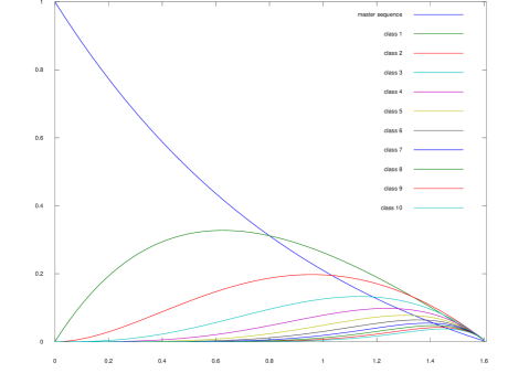
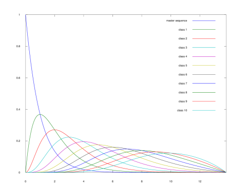
Some steps in this computation must be made rigorous, but this can done with a little extra work. In fact, this formula was obtained in [5], while studying the quasispecies arising in a stochastic model for the evolution of a finite population. Thanks to this formula, we can easily draw the quasispecies distribution (figures 2 and 2) and study its dependence on the parameters . In the quasispecies literature, this was previously done by integrating numerically the differential system (see for instance [8], figure 3, p.9). Besides, we can now perform simple theoretical computations with the help of this distribution. For instance, the mutation rate at which the proportion of the Hamming class becomes larger than the proportion of the wild type is .
13 Finitely many peaks
Now that we have well understood the case of the sharp peak landscape, we are ready to consider more complex landscapes. We still use the same genotype space and the same mutation kernel as for the sharp peak landscape and we make the following hypothesis on the fitness function .
Hypothesis 13.1.
There exist a fixed integer and fixed values such that: for any value of , there exist peaks in (whose localization may vary with and ) such that the fitness function is given by
| (13.2) |
We consider again the long chain regime
We shall prove the following theorem.
Theorem 13.3 (Error threshold for finitely many peaks).
Let us set
Let be the mean fitness for the model associated to the fitness function and the parameters . We have the following dichotomy:
If , then .
If , then .
We see that the situation is very similar to the case of the sharp peak landscape. The critical parameter depends now on the fitness of the highest peak. The conclusion is that a finite number of peaks do not really interfere with each other, and their respective contributions to the global equilibrium of the model are essentially independent.
As for the sharp peak landscape, we shall give two proofs of theorem 13.3, a soft one, whose starting point is the initial quasispecies equation, and a technical one, based on the strategy explained at the end of section 7. Again, the soft proof might look easier, but the technical proof is more informative and could potentially yield more accurate estimates. We define first the set of the wildtypes as
Throughout the proofs, we write simply or even instead of .
Soft proof.
We start as in the case of the sharp peak landscape. In the long chain regime, we have that . Using the lower bound (7.11) and the fact that , we see that
| (13.4) |
Suppose that does not converge towards . In this case, there exist and two sequences of parameters , such that
| (13.5) |
For , we bound from above the quasispecies equation (2.1) associated to , as follows:
| (13.6) |
We sum equation (13.6) over . Setting
we obtain
| (13.7) |
We use next the fact that whenever and we obtain that
Inserting these inequalities in (13.7), we obtain that
| (13.8) | ||||
| (13.9) |
In addition, we have that
| (13.10) |
Equation (13.10) and the condition (13.5) yield that
| (13.11) |
Using together (13.8) and (13.11), we obtain that
Sending to , we see that this inequality is not coherent with inequality (13.5). Therefore it must be the case that converges towards . ∎
Technical proof.
For this proof, we shall implement the strategy explained at the end of section 7. So we consider the matrix defined by
| (13.12) |
The advantage is that the size of the matrix is and it does not vary with and . The diagonal elements of the matrix are given by
In fact, the above series does not depend on . Using formula (8.6) with , we have
| (13.13) |
where is a binomial random variable with parameters . The parameter is adjusted so that the Perron–Frobenius eigenvalue of the matrix is equal to . This Perron–Frobenius eigenvalue is always larger or equal than any diagonal element, thus we must have . Proceeding exactly as in the technical proof of theorem 11.2, we obtain with the help of Jensen’s inequality that
| (13.14) |
Taking the maximum over , we get
| (13.15) |
We seek next an upper bound on the value of . The Perron–Frobenius eigenvalue of the matrix is equal to , and all its entries are non-negative, thus
In particular, there exists an index such that
| (13.16) |
Let us study the non-diagonal elements of the matrix . For , we have
In fact, the series depends only on the Hamming distance between and , as we can see from formula (8.3). The same formula shows also that is a non-increasing function of . Therefore, using the formula (8.16) with , we have the inequality
| (13.17) |
where is a binomial random variable with parameters . Moreover we know that , thus
| (13.18) |
Plugging (13.13) and (13.18) in inequality (13.16), we get (recall that )
| (13.19) |
We proceed in a way similar to what we did for the sharp peak landscape. Namely, we pick a positive number and we split the expectations according to the values of and , as follows:
| (13.20) |
We use the estimate given by Chebyshev’s inequality (10.4) and we obtain
| (13.21) |
We regroup the first and the third term together, as well as the second and the fourth term and we finally get (using that and that )
| (13.22) |
By making an adequate choice for , we shall now deduce an upper bound on from this inequality.
Lemma 13.23.
There exists a positive constant such that, in the long chain regime, the mean fitness satisfies
| (13.24) |
Proof.
Suppose that is larger than the upper bound in (13.24). We check that this is not compatible with inequality (13.22) with the choice . Indeed, we have on one hand
On the other hand,
We have also that
Combining the previous inequalities, we obtain that the right-hand member of inequality (13.22) has the following expansion:
This quantity becomes strictly less than for large enough, and this is not compatible with the inequality (13.22). ∎
14 Plateau
We have seen that a finite number of peaks do not interact significantly with each other. We consider here a fitness landscape which contains a kind of plateau, that is a large subset of genotypes having a fitness . More precisely, we consider the genotype space of binary sequences and the usual mutation kernel . To simplify the formulas, we suppose that the length is even. The Hamming class of is the number of one’s present in , that is
We consider the fitness function defined as follows.
Hypothesis 14.1.
The fitness function is given by
| (14.2) |
We consider again the long chain regime
Theorem 14.3.
Let be the mean fitness for the model associated to the fitness function and the parameters . For any , we have
where is the unique real number such that
| (14.4) |
The situation with the fitness landscape with the huge plateau is very different from the sharp peak landscape. Indeed, the error threshold phenomenon described in theorem 11.2 does not occur, and there is no phase transition in the long chain regime.
Proof.
We start by proving that equation (14.4) admits a unique solution. Let us define the function by
| (14.5) |
For any , we have
It follows that the map
is continuous decreasing on . Moreover it converges to when goes to and to when goes to , because
Thus there exists a unique value satisfying equation (14.4). We prove next the main claim of the theorem. Throughout the proof, we write simply or even instead of . We are dealing with a fitness function which depends only on the Hamming classes. So we lump together the genotypes according to their Hamming classes and we introduce the new variables , , given by
Using formula (7.7), we have
| (14.6) |
Now, the point is that the most inner sum depends only on the Hamming class of . Indeed, let us fix and let be such that . After mutation cycles on , we obtain a genotype whose components are independent Bernoulli random variables. Among them, exactly have parameter and have parameter (this is a consequence of the computations performed in section 4). Therefore the Hamming class of is distributed as the sum of two independent binomial random variables with respective parameters and . We conclude that
| (14.7) |
where the matrix is given by
| (14.8) |
being a generic binomial random variable with parameters and the two binomial random variables appearing above being independent. Rearranging the sum in formula (14.6) according to the Hamming class of and using (14.7), we get
| (14.9) |
This equation is in fact valid as long as the fitness function depends only the Hamming classes. In the case of the Plateau landscape, the equation for yields
| (14.10) |
This is the counterpart of equation (3.9) for the sharp peak landscape. We shall rely on this equation to analyze the asymptotic behavior of in the long chain regime. Let us begin with the term .
Lemma 14.11.
In the long chain regime, we have the convergence
| (14.12) |
where the sequence of functions is defined in (14.5).
Proof.
From formula (14.8) with , we have
with the understanding that the two binomial random variables appearing above are independent. Moreover, we have
hence we are in the regime where these binomial laws converge towards the Poisson distribution with parameter . Let us fix . We have
whence, passing to the limit,
Sending to , we obtain that
| (14.13) |
Let us look for the converse inequality. We fix again and we write
We bound the last term with the help of Markov inequality:
where the last inequality holds asymptotically. From the two previous inequalities, we conclude that
We finally send to to complete the proof of the lemma. ∎
We complete now the proof of theorem 14.3. Let be an accumulation point of . By definition, there exist two sequences of parameters , such that
By lemma 14.11 and Fatou’s lemma, we have
| (14.14) |
where the last equality comes from (14.10). This inequality and the very definition of (see equality (14.4)) imply that . In particular, there exists and such that
| (14.15) |
This last inequality ensures that the series
converges uniformly with respect to , so that we can interchange the limits and the infinite sum to get
This way we see that has to be the solution of equation (14.4). In conclusion, the only possible accumulation point for in the long chain regime is , therefore converges towards as announced. ∎
It turns out that, if we shift the Plateau away from , then an error threshold phenomenon reappears. We consider the fitness function defined as follows.
Hypothesis 14.16.
Let and . The fitness function is given by
| (14.17) |
where is the integer part of .
Theorem 14.18.
Suppose that . Let be the mean fitness for the model associated to the fitness function and the parameters . There exist two positive values such that: if , then
If , then
Of course, it would be more satisfactory to know that . This would be a consequence of the monotonicity of the function defined in (14.23), unfortunately this fact does not seem so obvious.
Proof.
We use a strategy similar to the one of the proof of theorem 14.3. The equation for in the system (14.9) yields
| (14.19) |
In the next lemma, we compute the asymptotic behavior of the quantity inside the sum.
Lemma 14.20.
In the long chain regime, we have the convergence
| (14.21) |
where the sequence of functions is defined by
| (14.22) |
Proof.
From formula (14.8) with , we have
with the understanding that the two binomial random variables appearing above are independent. Moreover, we have
hence we are in the regime where the first binomial law converges towards the Poisson distribution with parameter while the second binomial law converges towards the Poisson distribution with parameter . We proceed as in the proof of lemma 14.11 to conclude that
and we rewrite the right-hand quantity as in formula (14.22). ∎
Let be the function defined by
| (14.23) |
In order to study the behavior of as goes to or , we take advantage of the simple inequalities to bound from above and from below as follows:
From these inequalities, we deduce that, when , we have
| (14.24) |
Moreover, for any , we have
Thus, when , the series is uniformly convergent over for any and therefore the function is continuous on . We consider the equation
and we denote by (respectively ) the smallest (respectively the largest) solution to this equation in . These two real numbers are well-defined, thanks to the limits (14.24) and the continuity of on . Suppose that . Let be an accumulation point of . If , then, proceeding as in the proof of theorem 14.3, we pass to the limit along a subsequence in equation (14.19) to get
| (14.25) |
but this contradicts the fact that . Suppose that . Let be an accumulation point of . Suppose that . By Fatou’s lemma, we would have
| (14.26) |
where the last equality comes from (14.19). Yet inequality (14.26) stands in contradiction with the fact that . Therefore the infimum limit of has to be strictly larger than . ∎
The reason underlying this result is the following. In the neutral fitness landscape, the most likely Hamming class is already the class . By installing a Plateau precisely on this Hamming class, we reinforce its stability. When we shift the Plateau away from the Hamming class , we create a competition between two Hamming classes, and this leads to the occurrence of a phase transition.
15 Survival of the flattest
We will now combine the sharp peak landscape with a plateau. We consider the genotype space of binary sequences and the usual mutation kernel , with the following fitness function.
Hypothesis 15.1.
Let and let be the fitness function given by
| (15.2) |
We consider again the long chain regime
Theorem 15.3.
Let and let be the unique real number such that
| (15.4) |
Let be the mean fitness for the model associated to the fitness function and the parameters . We have the following convergence in the long chain regime:
Moreover, denoting by , the normalized Perron–Frobenius eigenvector associated to , we have the following cases:
If , then , .
If , then , .
Proof.
The mean fitness is also the Perron–Frobenius eigenvalue of the matrix . As such, it is a non-decreasing function of the entries of this matrix, therefore
With the help of theorems 13.3 and 14.3, we conclude that
Let us prove next the converse inequality. In the sequel of the proof, we write simply or even instead of . Let , be the normalized Perron–Frobenius eigenvector associated to , so that and satisfy
| (15.5) |
and moreover
| (15.6) |
and finally
As we saw previously, the system (15.5) is equivalent to the system (14.9). Let us rewrite the two equations of the system (14.9) corresponding to and :
| (15.7) | ||||
| (15.8) |
Let us examine what are the possible limits of , and along a subsequence in the long chain regime. So, let us suppose that, along a subsequence, the following convergences take place:
| (15.9) |
In the sequel of the argument, all the limits are taken along this subsequence. Passing to the limit in (15.6), we get
| (15.10) |
Since , then necessarily . Moreover, the following convergences take place:
| (15.11) |
while
| (15.12) |
The convergences (15.11) have already been proved, the first one is obvious and the second one is the purpose of lemma 14.11. To prove the convergences (15.12), we use the expression of computed in (14.8) and we get
and it is well–known that the right-hand quantities goes to as goes to . Proceeding as in the proof of theorem 14.3 (see lemma 14.11 and thereafter), we take advantage of the fact that to interchange the limit and the four sums appearing in (15.7). So, passing to the limit in (15.7), and using the convergences (15.9), (15.11), (15.12), we get
| (15.13) | ||||
| (15.14) |
If , then the first equation implies that . If , then the second equation is equivalent to equation (14.4), therefore has to be equal to the unique solution of this equation. In conclusion, there are only two possible limits along a subsequence for , namely and , thus
The final conclusions of the theorem are obtained as a by–product of the previous argument. Indeed, if , then it follows from (15.13) that we cannot have simultaneously and . This remark, in conjunction with the identity (15.10), yields the convergences stated at the end of the theorem. ∎
A plateau is always more stable than a peak of the same height, that is, for any , any , we have . However, for a fixed value , there exist positive values such that . Indeed, let us compute the right–hand member of equation (15.4) where is replaced by :
So, for any value of such that
we will indeed have . For such values, the quasispecies will be located on the plateau, despite the fact that the height of the plateau is strictly less than the height of the peak. In this situation, we witness the survival of the flattest.
References
- [1] Jon P. Anderson, Richard Daifuku, and Lawrence A. Loeb. Viral error catastrophe by mutagenic nucleosides. Annual Review of Microbiology, 58(1):183–205, 2004.
- [2] Alexander S. Bratus, Artem S. Novozhilov, and Yuri S. Semenov. Linear algebra of the permutation invariant Crow-Kimura model of prebiotic evolution. Math. Biosci., 256:42–57, 2014.
- [3] Alexander S. Bratus, Artem S. Novozhilov, and Yuri S. Semenov. On the behavior of the leading eigenvalue of Eigen’s evolutionary matrices. Math. Biosci., 258:134–147, 2014.
- [4] Alexander S. Bratus, Artem S. Novozhilov, and Yuri S. Semenov. Rigorous mathematical analysis of the quasispecies model: from Manfred Eigen to the recent developments. In Advanced mathematical methods in biosciences and applications, STEAM-H: Sci. Technol. Eng. Agric. Math. Health, pages 27–51. Springer, Cham, 2019.
- [5] Raphaël Cerf and Joseba Dalmau. The distribution of the quasispecies for a Moran model on the sharp peak landscape. Stochastic Process. Appl., 126(6):1681–1709, 2016.
- [6] Francisco M Codoñer, José-Antonio Darós, Ricard V Solé, and Santiago F Elena. The fittest versus the flattest: Experimental confirmation of the quasispecies effect with subviral pathogens. PLOS Pathogens, 2(12):1–7, 12 2006.
- [7] Shane Crotty, Craig E. Cameron, and Raul Andino. RNA virus error catastrophe: Direct molecular test by using ribavirin. Proceedings of the National Academy of Sciences, 98(12):6895–6900, 2001.
- [8] E. Domingo and P. Schuster. Quasispecies: From Theory to Experimental Systems. Current Topics in Microbiology and Immunology. Springer International Publishing, 2016.
- [9] Esteban Domingo and Celia Perales. Viral quasispecies. PLOS Genetics, 15(10):1–20, 10 2019.
- [10] Manfred Eigen. Self-organization of matter and the evolution of biological macromolecules. Naturwissenschaften, 58(10):465–523, 1971.
- [11] Manfred Eigen, John McCaskill, and Peter Schuster. The molecular quasi-species. Advances in Chemical Physics, 75:149–263, 1989.
- [12] P. Farci. New insights into the hcv quasispecies and compartmentalization. Seminars in liver disease, 31(4):356–374, 2011.
- [13] William Feller. An introduction to probability theory and its applications. Vol. I. John Wiley & Sons Inc., New York, 1968.
- [14] Joshua Franklin, Thomas LaBar, and Christoph Adami. Mapping the Peaks: Fitness Landscapes of the Fittest and the Flattest. Artificial Life, 25(3):250–262, 08 2019.
- [15] John G. Kemeny and J. Laurie Snell. Finite Markov chains. Springer-Verlag, New York, 1976. Undergraduate Texts in Mathematics.
- [16] J. F. C. Kingman. On the properties of bilinear models for the balance between genetic mutation and selection. Math. Proc. Cambridge Philos. Soc., 81(3):443–453, 1977.
- [17] A. Meyerhans, R. Cheynier, J. Albert, M. Seth, S. Kwok, J. Sninsky, L. Morfeldt-Mø anson, B. Asjö, and S. Wain-Hobson. Temporal fluctuations in hiv quasispecies in vivo are not reflected by sequential hiv isolations. Cell, 58(5):901–910, 1989.
- [18] Patrick A. P. Moran. Global stability of genetic systems governed by mutation and selection. Math. Proc. Cambridge Philos. Soc., 80(2):331–336, 1976.
- [19] Josep Sardanyés, Santiago F. Elena, and Ricard V. Solé. Simple quasispecies models for the survival-of-the-flattest effect: the role of space. J. Theoret. Biol., 250(3):560–568, 2008.
- [20] Héctor Tejero, Arturo Marín, and Francisco Montero. The relationship between the error catastrophe, survival of the flattest, and natural selection. BMC Evolutionary Biology, 11, 04 2011.
- [21] Claus O. Wilke, Jia Lan Wang, Charles Ofria, Richard E. Lenski, and Christoph Adami. Evolution of digital organisms at high mutation rates leads to survival of the flattest. Nature, 412:331–333, 07 2001.