Post-inflationary production of particle Dark Matter:
non-minimal Natural inflationary scenarios

Abstract

We investigate the production of non-thermal fermionic dark matter particles during the reheating era following slow roll inflation, driven by axion-like pseudo-Nambu-Goldstone boson, $\varphi$, that is non-minimally coupled to the curvature scalar, ${\cal R}$. We consider two types of non-minimal coupling, one of which is $\xi\varphi^{2}{\cal R}$ (referred to as NM-N), and the other one is $\alpha\left(1+\cos\left(\frac{\varphi}{f_{a}}\right)\right)$ (referred to as NMP-N), where $\alpha$ and $\xi$ are dimensionless parameters and $f_{a}$ is an energy scale. We determine benchmark values for both inflationary scenarios satisfying current bounds from Cosmic Microwave Background (CMB) radiation measurement and find the mass of inflaton to be $\sim{\cal O}\quantity(10^{12})\,\text{GeV}$ for both inflationary scenarios and tensor-to-scalar ratio, $r\sim 0.0177$ (for NM-N) and $\sim 0.0097$ (for NMP-N) which fall inside $1-\sigma$ contour on scalar spectral index versus $r$ plane of Planck2018+Bicep3+Keck Array2018 joint analysis, and can be probed by future CMB observations e.g. Simons Observatory. We then show that dark matter particles produced from the decay of inflaton can fully match the present-day cold dark matter (CDM) yield, as well as other cosmological constraints, if the coupling value between inflaton and dark matter, $y_{\chi}$, and the dark matter mass, $m_{\chi}$, are within the range $10^{-6}\gtrsim y_{\chi}\gtrsim 10^{-17}$ and ${\cal O}\quantity(1\,\text{GeV})\lesssim m_{\chi}\lesssim m_{\phi}/2$, where $m_{\phi}$ denotes the mass of inflaton. The exact range of $y_{\chi}$ and $m_{\chi}$ varies with different benchmark values as well as parameters of inflation, like energy scale of inflation and $r$, some of which are within the reach of next generation CMB experiments.

I Introduction

Big bang cosmological model has been widely accepted model describing the origin of the universe, with evidence such as the Hubble expansion of distant galaxies and the Cosmic Microwave Background (CMB) radiation supporting its validity. However, precise analysis of the CMB data suggests that our universe is nearly spatially flat, homogenous, and isotropic on large scales, with nearly uniform temperature of CMB photons ($2.75\,\text{K}$) which are difficult to reconcile with the Big Bang Model. On the other hand, Big Bang model suggests that if we trace back in time from the current state of the expanding and cold universe, it would contract into a point with extremely high energy during its origin, and the universe is expanding ever since, with varying expansion rates during different cosmological epochs. Cosmological inflation is one of the primeval epochs that occurs for a very short time during which the energy density of the universe is dominated by that of inflaton, and consequently, space-time expands exponentially. This epoch successfully addresses most of the shortcomings of Big Bang model. During this epoch, the Hubble radius remained almost constant, and due to the finite size of the observable universe, it is expected that quantum relic scalar and tensor perturbations are generated, which at a later stage plays crucial role in the structure formation, generation of relic gravitational waves, and perhaps even in the formation of primordial black holes. This epoch was first introduced in literature by Refs. Starobinsky (1980); Guth (1981); Linde (1982); Albrecht and Steinhardt (1982). Since then, this epoch has become so popular that numerous inflationary models have been proposed in the literature. However, analyses of the latest data from Planck and BICEP observations Akrami et al. (2020); Ade et al. (2018) have resulted in a reassessment of the preferred feasible inflation models. Multi-field inflationary scenarios that involve non-negligible coupling between the light scalars during inflation are in tension due to the absence of large non-Gaussianities in the CMB  data Folkerts et al. (2014). On the other hand, several single field inflation scenarios, including slow roll chaotic inflation with potential of monomial form ($V(\phi)\propto\phi^{p}$, specifically with $p=1,2,4$), large field inflation with field value greater than Planck mass are ruled out even by $2-\sigma$ on the $(n_{s},r)$ plane (see e.g., Ref. Martin et al. (2014) for a comprehensive review). However, with non-minimal coupling to gravity (Ricci scalar $\mathcal{R}$) several inflationary models can be revived with suitable choice of the coupling Hertzberg (2010).

Among other unresolved issues of the Big Bang model is the understanding of the origin and composition of dark matter (DM) and it remains one of the biggest mysteries. CMB data manifests that $26.5\%$ of the total mass-energy density of the universe is in the form of CDM. Despite the existence of numerous gravitational interactions of DM in addition to the CMB data, there has not been any direct evidence of non-gravitational signatures of DM to date. As a result, the identity of DM and how it came to exist in the universe remain unknown Bertone et al. (2005). Several hypotheses have been proposed to explain the mechanism of DM production during different cosmological epochs Bernal et al. (2018a). The interaction channels through which DM particles are produced, together with its cross-section with other particles, control the decoupling time from the Standard Model (SM) relativistic plasma of the universe. In this study, we focus on the production of DM during one of the earliest cosmological epoch, specifically, during the reheating era . Among non-thermal DMproduction scenarios, Feebly Interacting Massive Particles (FIMP) McDonald (2002); Choi and Roszkowski (2005); Kusenko (2006); Petraki and Kusenko (2008); Hall et al. (2010); Bernal et al. (2017) may be a viable option, owing to their significantly weaker interactions, which prevent them from attaining thermal equilibrium with relativistic plasma in the early universe. In contrast to WIMP, the number density of FIMP depends on initial conditions. FIMP DM particles can be formed mainly in three ways: first, their number density freezes as soon as the temperature of the relativistic plasma drops below the mass of the DM particles. Second, they can be produced from the decay of heavy particles such as moduli fields, the curvaton (see, e.g. Ref. Baer et al. (2015)), or the inflaton which is considered in this work. Third, they can be generated through the scattering of SM particles mediated by inflaton or graviton Garny et al. (2016); Tang and Wu (2016, 2017); Garny et al. (2018); Bernal et al. (2018b). Recently several scenarios involving testability of FIMP DM involving long-lived particles at laboratories Barman et al. (2023, 2022a); Barman and Ghoshal (2022a); Barman et al. (2022b); Barman and Ghoshal (2022b); Ghosh et al. (2023) and involving primordial Gravitational Waves of cosmological origin have been proposed Ghoshal et al. (2022a); Berbig and Ghoshal (2023); Paul et al. (2019); Ghoshal and Saha (2022).

In this work, alongside with Ref. Ghoshal et al. , we present a scenario where the DM particles are non-thermal and produced from the inflaton during the reheating era which is preceded by single-field natural inflation where inflaton is non-minimally coupled to Ricci scalar. For the inflationary part, we have considered natural inflation motivated by cosine potential of axion-like particles in general. We derive the conditions on DM parameter space from the inflationary constraint analysis and DM phenomenology constraints on inflaton DM couplings and inflaton and DM masses.

The paper is organized as follows: we present the action of our model in Sec. II. Next, in Secs. III and IV, we explore two inflationary scenarios: non-minimal natural inflation with both $\xi\varphi^{2}{\cal R}$ and periodic non-minimal coupling. For each inflationary scenario, we study the slow-roll inflation, reheating, and production of dark matter (DM). In  Sec. V, we summarize our findings.

We use $\hbar=c=k_{B}=1$ unit throughout this paper, such that the value of reduced Planck mass is $M_{P}=2.4\times 10^{18}\,\text{GeV}$. We also consider that the space-time metric is diagonal with signature $(+,-,-,-)$.

II Lagrangian density

In this analysis, we assume that the inflationary epoch in the early universe is driven by an axion or axion-like pseudo-Nambu–Goldstone boson, $\varphi$, which is singlet under SM gauge transformations, and the inflaton is non-minimally coupled to gravity. Therefore, the action of inflaton in Jordan frame is given by Nozari and Sadatian (2008); Cheong et al. (2022); Kodama and Takahashi (2022)

$${\cal S}^{JF}\supset\int\text{d}^{4}x\sqrt{-g^{JF}}\left(\frac{1}{2}M_{P}^{2}\,\Omega^{2}(\varphi)\,{\cal R}^{JF}+\frac{1}{2}\left(\partial\varphi\right)^{2}-V^{JF}(\varphi)\right)\,,$$ (1)

where the notion $JF$ in superscript denotes that the associated parameter is defined in Jordan frame, for example, $g^{JF}$ and ${\cal R}^{JF}$ represent the determinant of space-time metric and Ricci scalar, respectively, in Jordan frame. Here, $\varphi$ is the inflaton in Jordan frame, $\Omega^{2}(\varphi)\equiv\Omega^{2}\neq 0$, and the inflationary potential in Jordan frame is

$$V^{JF}(\varphi)=\Lambda^{4}\left(1+\cos\left(\frac{\varphi}{f_{a}}\right)\right)\,,$$ (2)

where $\Lambda$ and $f_{a}$ are energy scales that are described in more detail later. Now, by conformally transforming the space-time metric in Jordan frame, we can derive the space-time metric in Einstein frame as

$$g^{E}_{\mu\nu}=\Omega^{2}\,g^{JF}_{\mu\nu}\,.$$ (3)

Hereafter, we use superscript $E$, which implies that the associated parameter is defined in Einstein frame. In this fame, the gravity sector is canonical. Therefore, the action in Einstein frame is

$${\cal S}^{E}\supset\int\text{d}^{4}x\sqrt{-g^{E}}\left(\frac{1}{2}M_{P}^{2}\,{\cal R}^{E}+\frac{1}{2}\Pi(\varphi)\left(\partial\varphi\right)^{2}-\Omega^{-4}\,V^{JF}(\varphi)\right)\,,$$ (4)

where Shaposhnikov et al. (2020)

$$\Omega^{2}(\varphi)=1+\frac{F(\varphi)}{M_{P}^{2}}\,,\qquad\Pi(\varphi)\equiv\frac{1}{\Omega^{2}}+\kappa\,\frac{3}{2M_{P}^{2}}\frac{1}{\Omega^{4}}\left(\frac{\text{d}F(\varphi)}{\text{d}\varphi}\right)^{2}\,,$$ (5)

along with $\kappa=1$ (metric formalism). To express the kinetic energy of the inflaton in canonical form, we need to redefine the inflaton as

$$\frac{d\phi}{d\varphi}=\sqrt{\Pi(\varphi)}\,.$$ (6)

Hence, $\phi$ is the inflaton in Einstein frame. The value of $\phi$ as a function of $\varphi$ can be found using Eq. 6. The action of Eq. 4 then transforms as

$${\cal S}^{E}\supset\int\text{d}^{4}x\sqrt{-g^{E}}\left(\frac{1}{2}M_{P}^{2}\,{\cal R}^{E}+\frac{1}{2}\left(\partial\phi\right)^{2}-V^{E}(\phi)\right)\,,$$ (7)

where the potential of the inflaton in Einstein frame is

$$V^{E}(\phi)=\frac{V^{JF}\left(\varphi(\phi)\right)}{\Omega^{4}\left(\varphi(\phi)\right)}\,.$$ (8)

For slow roll inflation in Einstein frame, the first two potential slow roll parameters are defined as Oda et al. (2018); Järv et al. (2017); Kodama and Takahashi (2022)

$$\epsilon_{V}^{E}=\frac{M_{P}^{2}}{2}\quantity(\frac{\text{d}\ln[V^{E}]}{\text{d}\varphi}\frac{\text{d}\varphi}{\text{d}\phi})^{2}\,,$$ (9)

$$\eta_{V}^{E}=M_{P}^{2}\quantity(\frac{1}{V^{E}}\frac{\text{d}^{2}V^{E}}{\text{d}\varphi^{2}}\left(\frac{\text{d}\varphi}{\text{d}\phi}\right)^{2}-\frac{\text{d}\ln[V^{E}]}{\text{d}\varphi}\frac{\text{d}^{2}\phi}{\text{d}\varphi^{2}}\left(\frac{\text{d}\varphi}{\text{d}\phi}\right)^{3})\,.$$ (10)

Both of these $\epsilon_{V}^{E}$ and $\left|\eta_{V}^{E}\right|$ should be $<1$ to continue the slow roll phase, and this ensures that the inflaton is over damped and Hubble parameter, ${\cal H}$, remains nearly constant during inflation Lyth (1993). The slow roll phase ceases whenever at least one of these two parameters reaches $\sim 1$. During slow roll inflation, nearly constant value of ${\cal H}$ (quasi-de Sitter) and exponential growth of cosmological scale factor $\boldsymbol{a}$ implies that comoving Hubble radius ($\quantity(\boldsymbol{a}{\cal H})^{-1}$) shrinks exponentially, resulting in comoving length scales possibly leaving the Hubble horizon. Thus, if there are two length scale $k_{*}$ and $k_{\rm end}$ that exit the casual horizon just at the beginning and end of inflation, then the number of e-folds by which $\boldsymbol{a}$ is increased during this time is Oda et al. (2018)

$${\cal N}_{\text{CMB}}=\frac{1}{M_{P}}\int_{\varphi_{{\rm end}}}^{\varphi_{*}}\text{d}\varphi\;\frac{1}{\sqrt{2\,\epsilon_{V}^{E}}}\left(\frac{\text{d}\phi}{\text{d}\varphi}\right)\,,$$ (11)

where $\varphi_{*}$ and $\varphi_{{\rm end}}$ are the values of inflaton corresponding to when $k_{\star}$ and $k_{\rm end}$ leave the horizon. If the length scale $k_{*}$ reenters within the Hubble radius today and Cosmic Microwave Background (CMB) observations are measured, then at least ${\cal N}_{\text{CMB}}\sim 60$ Baumann (2022) ($k_{*}\sim 0.05\,\text{Mpc}^{-1}$) (or ${\cal N}_{\text{CMB}}\gtrsim 66-70$, depending on inflationary model Bambi and Dolgov (2015)) is required to solve the horizon problem.

Because of the finite size of ${\cal H}$, scalar and tensor quantum perturbations are expected to be generated during slow roll inflationary phase. The exponential expansion during inflation stretches the wavelengths of the quantum perturbations even beyond the Hubble horizon. Those perturbations upon reentering the horizon, is measured in terms of two point correlation function i.e. power spectrum which are defined as

$$\mathcal{P}_{s}\left(k\right)=A_{s}\left(\frac{k}{k_{*}}\right)^{n_{s}-1+(1/2)\alpha_{s}\ln(k/k_{*})+(1/6)\beta_{s}(\ln(k/k_{*}))^{2}}\,,$$ (12)

$$\mathcal{P}_{h}\left(k\right)=A_{t}\left(\frac{k}{k_{*}}\right)^{n_{t}+(1/2)dn_{t}/d\ln k\ln(k/k_{*})+\cdots}\,,$$ (13)

where $k_{*}$ is the pivot scale at which bounds on inflation are measured from the analysis of CMB data, and

• $\mathcal{P}_{s}$ and $\mathcal{P}_{h}$ : scalar and tensor power spectrum of primordial perturbation,

• $A_{s}$ and $A_{t}$: amplitude of scalar and tensor power spectrum,

• $n_{s}$ and $n_{t}$: scalar and tensor spectral index,

• $\alpha_{s}$ and $\beta_{s}$: running and running of running of scalar spectral index.

For the given single-field inflationary potential $A_{s}$ and $n_{s}$ can be measured as

$$A_{s}\approx\frac{1}{24\pi^{2}}\frac{1}{M_{P}^{4}}\left.\frac{V^{E}}{\epsilon_{V}^{E}}\right|_{k=k_{\star}}\,, n_{s}(\varphi_{*})=1-6\,\epsilon_{V}^{E}(\varphi_{*})\,+\,2\,\eta_{V}^{E}(\varphi_{*})\,.$$ (14)

For $n_{s}<1$, $\mathcal{P}_{s}$ is red tilted i.e. more power at larger length scales. Now, if we define tensor-to-scalar ratio $r=A_{t}/A_{s}$, then Akrami et al. (2020)

$$V^{E}(\varphi_{*})=\frac{3}{2}\pi^{2}\,r(\varphi_{*})\,A_{s}\,M_{P}^{4},$$ (15)

where we have used slow roll approximation $r(\varphi_{*})\approx 16\,\epsilon_{V}^{E}(\varphi_{*})$. Current CMB constraints on $A_{s}$, $n_{s}$, and $r$ are mentioned in Table 1.

Table 1: Constraints on inflationary parameters from Planck, Planck+Bicep+Keck Array and other CMB experiments (T and E for temperature and E-mode polarization of CMB).

$\ln(10^{10}A_{s})$	$3.044\pm 0.014$	$68\%$, TT,TE,EE+lowE+lensing+BAO	Aghanim et al. (2020); Workman et al. (2022)
$n_{s}$	$0.9647\pm 0.0043$	$68\%$, TT,TE,EE+lowE+lensing+BAO	Aghanim et al. (2020)
$r$	$0.014^{+0.010}_{-0.011}\,\text{and}$	$95\%\,,\text{BK18, {Bicep}3, {Keck Array}~{}2020,}$	Aghanim et al. (2020); Ade et al. (2022a, 2021)
	$<0.036$	and WMAP and Planck CMB polarization	(see also Campeti and Komatsu (2022))

In addition to the slow roll inflationary epoch, in this article, we also consider the reheating era that comes after inflation, and also make the assumption that during that reheating era production of non-thermal DM particles and SM Higgs proceeds concomitantly. Therefore, the total action in which we are interested in can be expressed as follows Bernal and Xu (2021); Ghoshal et al. (2022b, 2023a, c)

$${\cal S}_{\rm tot}\supset{\cal S}^{E}+\int\text{d}x^{4}\sqrt{-g^{E}}\,\left({\cal L}_{\chi}^{E}+{\cal L}_{H}^{E}+{\cal L}_{{\rm rh}}^{E}\right)\,.$$ (16)

Here, the Lagrangian density of the beyond the standard model (BSM) vector-like fermionic field $\chi$ and SM Higgs doublet $H$ are ${\cal L}_{\chi}$ and ${\cal L}_{H}$, respectively, and those can be written in the following form:

$${\cal L}_{\chi}^{E} =i\bar{\chi}\not{\partial}\chi-m_{\chi}\bar{\chi}\chi\,,$$ (17)

$${\cal L}_{H}^{E} =\left(\partial H\right)^{2}+m_{H}^{2}H^{\dagger}H-\lambda_{H}\left(H^{\dagger}H\right)^{2}\,,$$ (18)

where both the parameters $m_{\chi}$ and $m_{H}$ have the mass dimension whereas the parameter $\lambda_{H}$ is dimensionless. Moreover, ${\cal L}_{\rm rh}^{E}$ in Eq. 16 comprises interaction between the inflaton and the dark sector as well as between the inflaton and SM Higgs. Hence,

$$\mathcal{L}_{{\rm rh}}^{E}=-y_{\chi}\phi\bar{\chi}\chi-\lambda_{12}\phi H^{\dagger}H-\lambda_{22}\phi^{2}H^{\dagger}H+{\cal L}_{\rm scatter}+\text{h.c.}\,.$$ (19)

where ${\cal L}_{\rm scatter}$ includes higher order terms that account for the scattering of $\chi$ by inflaton, or SM particles (including $H$). The couplings $y_{\chi}$ and $\lambda_{22}$ are also dimensionless, but $\lambda_{12}$ has mass dimension. In the two succeeding sections (Secs. III and IV), we consider two different forms of $\Omega^{2}(\varphi)$, and study the slow roll single field inflationary scenarios, and determine benchmark values that satisfy the current CMB bounds. We also investigate the parameter space, involving $y_{\chi}$ and $m_{\chi}$ under the assumption that the total CDM density of the present universe is completely comprised of $\chi$ particles produced during the reheating era.

III Natural inflation with $\xi\varphi^{2}{\cal R}$ non-minimal coupling

Natural inflation with canonical kinetic energy term is no longer the favorite candidate for single field inflationary scenario since this model predicts large values of $r$ relative to $2-\sigma$ best-fit contour from Planck 2018+Bicep data on $n_{s}-r$ plane Akrami et al. (2020); Ghoshal et al. (2023b). However, this is one of the inflationary models which has strong motivation based on particle physics theory. In this theory, inflaton is an axion or axionic field which is a pseudo-Nambu-Goldstone boson, arising from the spontaneous breaking of global symmetry and an additional subsequent explicit symmetry breaking. This boson is introduced in the theory to solve strong CP problem Peccei (2008); Hook (2019); Kim and Carosi (2010). The axion potential which arises non-perturbatively due to the spontaneous breaking of global $U(1)$ symmetry can be written in the form similar to that presented in Eq. 2 (with $\xi=0$) where $\varphi$ represents the canonically normalized axion or axionic field. Here $\Lambda$ is the $U(1)$ explicit symmetry-breaking energy scale of the continuous shift symmetry, while $f_{a}$ determines the spontaneous U(1) symmetry-breaking energy scale. Additionally, $f_{a}$ is accountable for the small value of self-coupling as $f_{a}$ reduces its value by $1/f_{a}$ and, hence, solves the problem of fine-tuning. For this reason, this inflationary model is called natural inflation. Furthermore, this potential has a shift symmetry ($V(\varphi)=V(\varphi+\text{const.})$) and thus protects the flatness of the potential. On the other hand, the shift symmetry protects the flatness of the potential of axion-inflaton Kim et al. (2005); Freese et al. (1990).

Being such a theoretically well-motivated model Savage et al. (2006), several attempts have been made to modify the theory slightly so that the predicted value of $r$ remains within at least $2-\sigma$ contour of Planck data. Additionally, another objective has been to reduce the value of $f_{a}$ (the range of $f_{a}$ used in the paper of Planck collaboration is $10\lesssim f_{a}/M_{P}\lesssim 1585$). Some of these attempts includes Cheng et al. (2021) which considers generalized versions of natural inflation, Daido et al. (2017) which explores the incorporation of multiple axion-like fields. However, in this section, we consider the inflationary model presented in Ref. Reyimuaji and Zhang (2021) where a non-minimal coupling between the inflaton and gravity sector has been considered, and non-minimal coupling has the following form :

$$\Omega^{2}(\varphi)=1+\xi\frac{\varphi^{2}}{M_{P}^{2}}\,,$$ (20)

where $\xi$ is dimensionless non-minimal coupling between $\varphi$ and gravity. This coupling can be arisen at 1-loop order from quantum corrections in curved spacetime Birrell and Davies (1984); Faraoni (1996), and for the theoretical motivation of such form of non-minimal coupling see Refs. Hertzberg (2010); Hrycyna (2017). For this coupling, from Eq. 6 we get

$$\frac{\text{d}\phi}{\text{d}\varphi}=\sqrt{\frac{\xi(6\xi+1)\varphi^{2}M_{P}^{2}+M_{P}^{4}}{\left(M_{P}^{2}+\xi\varphi^{2}\right){}^{2}}}$$ (21)

Moreover, the potential $V^{JF}(\varphi)$ has local maxima at $\varphi=nf_{a}\pi$ ($n=0,2,4,\ldots$) and local minima at $\varphi=nf_{a}\pi$ ($n=1,3,5,\ldots$). The potential of non-minimal Natural (abbreviated as NM-N) Inflation in Einstein frame is

$$V^{E}(\phi(\varphi))\equiv V^{E}_{\text{NM-N}}(\phi(\varphi))=\frac{\Lambda^{4}\left(1+\cos\left(\frac{\varphi}{f_{a}}\right)\right)}{\quantity(1+\xi\,\varphi^{2}/M_{P}^{2})^{2}}$$ (22)

For this inflationary model in metric formalism, the benchmark values are presented in Table 2. The value of $f_{a}/M_{P}\sim{\cal O}\quantity(1)$ is required for $n_{s}\sim 0.9647$ which is much smaller than the value of $f_{a}/M_{P}$ required for minimal natural inflationary scenario. Following Ref. Reyimuaji and Zhang (2021), we choose negative value of $\xi$ such that $n_{s}$ remains within $1-\sigma$ best fit contour from Planck 2018 data. The lower bound on $\xi$ comes from the condition $\left(1+\xi\quantity(\varphi_{\rm min}/M_{P})^{2}\right)>0$. The predicted $n_{s},r$ values of the three benchmarks from Table 2 are shown in Fig. 1, along with bounds from current CMB observations (Planck+Bicep+Keck Array) and future prospective reaches from other upcoming CMB observations. Predicted value of $r$ of benchmark ‘(m)NM-N-1’ is within $2-\sigma$ contour of Planck2018+Bicep3 (2022)+Keck Array2018 data, while predicted value of $r$ of benchmark ‘(m)NM-N-2’ is within $2-\sigma$ contour Planck2018 data. On the other hand, benchmark ‘(m)NM-N-3’ shows that for NM-N inflation and for a slightly larger value of e-folds (e.g. ${\cal N}_{\text{CMB}}\sim 70$) predicted $r$ value falls even within $1-\sigma$ best-fit contour of Planck2018+Bicep3 (2022)+Keck Array2018 combined analysis.

Table 2: Benchmark value for NM-N inflationary model in metric formalism ($\varphi_{\rm min}$ is the location of minimum).

Benchmark	$f_{a}/M_{P}$	$\xi$	$\varphi_{*}/M_{P}$	$\varphi_{\rm end}/M_{P}$	$n_{s}$	$r\times 10^{2}$	$\Lambda^{4}/M_{P}^{4}$	$\varphi_{\rm min}/M_{P}$	${\cal N}_{\text{CMB}}$
(m)NM-N-1	$3.01$	$-10^{-2}$	$3.5140$	$9.1132$	$0.9647$	$2.4841$	$4.2633\times 10^{-10}$	$9.4430$	$60$
(m)NM-N-2	$8.00$	$2\times 10^{-6}$	$10.7614$	$23.7212$	$0.9645$	$7.9452$	$2.0184\times 10^{-9}$	$25.1327$	$60$
(m)NM-N-3	$3.00$	$-10^{-2}$	$2.9562$	$9.0878$	$0.9658$	$1.7702$	$2.9508\times 10^{-10}$	$9.4248$	$70$

Figure 1: The colored dots represent the predicted values of $(n_{s},r)$ for benchmark values from Table 2. Alongside, this figure also displays $95\%$ C.L. ($1-\sigma$) contours highlighted by a deep-colored regions located inside and $68\%$ C.L. ($2-\sigma$) $(n_{s},r)$ best-fit contours as light-colored regions located outside. The green colored region is for best-fit bound from Planck 2018 while the blue shaded area presents bound from Planck 2018+Bicep3 (2022)+Keck Array2018 joint analysis. Other colored regions, with dashed lines as periphery, show contours from different forthcoming CMB observations (LiteBIRD+CMB-S4+Simons Observatory (SO)) Hazumi et al. (2020); Abazajian et al. (2016); Ade et al. (2019).

III.1 Reheating

The reheating phase commences once the slow roll phase ends. During this time, the inflaton field reaches the minimum of its potential, which is also its vacuum expectation value. The inflaton then proceeds to oscillate quasi-periodically around this minimum. In this work we are assuming that potential about the minimum during the reheating era can be approximated as $V^{E}\sim\phi^{2}$ such that energy density of oscillating inflaton and pressure averaging over an oscillating cycle during reheating, behaves as Enqvist (2012) (see also Garcia et al. (2020))

$$\rho_{\phi}\propto\boldsymbol{a}^{-3}\,,\qquad \left<p\right>=0\,,$$ (23)

But in addition to the expansion of the universe, the production of SM and BSM particles from the inflaton also causes the energy density of inflaton to decrease. Reheating epoch is profoundly adiabatic and transforms the universe from being cold and dominated by the energy density of inflaton into being hot and dominated by SM radiation. Therefore, we can safely assume that

$$\Gamma_{\phi}=\Gamma_{\phi\to{hh}}+\Gamma_{\phi\to\chi\chi}\approx\Gamma_{\phi\to{hh}}\,.$$ (24)

where $\Gamma_{\phi},\Gamma_{\phi\to{hh}},$ and $\Gamma_{\phi\to\chi\chi}$ are respectively the total decay width of inflaton, decay width of inflaton to SM Higgs particle $h$ and decay width of inflaton to DM particle $\chi$. There is no need for an explicit coupling between $\varphi$ and those particles to be produced in $f(\varphi){\cal R}$ theories Watanabe and Komatsu (2007) or DM particles can be produced gravitationally (see Refs. Kannike et al. (2017); Babichev et al. (2020); Cembranos et al. (2020); Bambi and Dolgov (2015)). In this work, however, we take advantage of the perturbative reheating technique and particle creation in Einstein frame using Eq. 19. Neglecting the effect of thermal mass Kolb et al. (2003), we can find $\Gamma_{\phi\to{hh}},$ and $\Gamma_{\phi\to\chi\chi}$ from Eq. 19 as

$$\Gamma_{\phi\to{hh}}\simeq\frac{\lambda_{12}^{2}}{8\pi\,m_{\phi}}\,,\qquad\Gamma_{\phi\to\chi\chi}\simeq\frac{y_{\chi}^{2}\,m_{\phi}}{8\pi}\,,$$ (25)

where the physical mass of the inflaton in Einstein frame is

$$\frac{m_{\phi}}{M_{P}}=\left(\frac{1}{M_{P}^{2}}\left.\frac{\text{d}^{2}V^{E}(\phi)}{\text{d}\phi^{2}}\right|_{\phi=\phi_{\rm min}}\right)^{1/2}\,.$$ (26)

Here, $\phi_{\rm min}$ is the location of the minimum of the potential of Eq. 22. Now, let us define the maximum possible temperature during reheating, $T_{max}$, and reheating temperature, $T_{\rm rh}$, as Bernal and Xu (2021); Giudice et al. (2001); Chung et al. (1999)

$$T_{max}= \Gamma_{\phi}^{1/4}\left(\frac{60}{g_{\star}\,\pi^{2}}\right)^{1/4}\left(\frac{3}{8}\right)^{2/5}{\cal H}_{I}^{1/4}M_{P}^{1/2}\,,$$ (27)

$$T_{\rm rh}= \sqrt{\frac{2}{\pi}}\left(\frac{10}{g_{\star}}\right)^{1/4}\sqrt{M_{P}}\sqrt{\Gamma_{\phi}}\,.$$ (28)

The production of SM particles by the inflaton causes the temperature of the universe to increase once the reheating epoch starts. This temperature reaches its maximum value, $T_{max}$, and then decreases as a result of the expansion of the universe. When the temperature of the universe drops to $T\sim T_{\rm rh}$, it then occurs that $\Gamma_{\phi}\sim{\cal H}(T_{\rm rh})$. At this moment, $\rho_{\rm rad}=\rho_{\phi}$, where $\rho_{\rm rad}$ is the energy density of SM relativistic particles i.e. radiation. The universe then shifts to being dominated by radiation, and remaining energy density of inflaton rapidly and quickly transforms mostly to $\rho_{\rm rad}$. In Eqs. 27 and 28 $g_{\star}$ is the effective number of relativistic degrees of freedom which is taken as $g_{\star}=106.75$ (being feebly interacting, $\chi$ might not have the same temperature as that of SM radiation), and in Eq. 27, ${\cal H}_{I}$ is the value of Hubble parameter at the end of inflation (i.e. when $\rho_{\rm rad}=0$ Giudice et al. (2001))

$${\cal H}_{I}=\sqrt{\frac{V^{E}\quantity(\phi\quantity(\varphi_{\rm end}))}{3M_{P}^{2}}}\,.$$ (29)

Following Eqs. 28, 24 and 29, we can calculate $\Gamma_{\phi}$, $T_{\rm rh}$, ${\cal H}_{I}$, and those values are mentioned in Table 3. The value of $m_{\phi}$ is highest for the benchmark ‘(m)NM-N-1’ and lowest for ‘(m)NM-N-2’, while the value of ${\cal H}_{I}$ is the highest for ‘(m)NM-N-1’.

Table 3: $m_{\phi},\Gamma_{\phi},T_{\rm rh}$, and ${\cal H}_{I}$ for the benchmark values from Table 2.

Benchmark	$m_{\phi}/M_{P}$	$\Gamma_{\phi}\,M_{P}$	$T_{\rm rh}/\lambda_{12}$	${\cal H}_{I}/M_{P}$
	(Eq. (26))	(Eq. (24))	(Eq. (28))	(Eq. 29)
(m)NM-N-1	$1.7078\times 10^{-5}$	$2329.89\,\lambda_{12}^{2}$	$21.3067$	$5.4539\times 10^{-6}$
(m)NM-N-2	$5.6123\times 10^{-6}$	$7089.55\,\lambda_{12}^{2}$	$37.1670$	$3.2284\times 10^{-6}$
(m)NM-N-3	$1.4095\times 10^{-5}$	$2822.91\,\lambda_{12}^{2}$	$23.4529$	$4.5216\times 10^{-6}$

From Eqs. 27 and 28 we can derive

$$\frac{T_{max}}{T_{\rm rh}}=\left(\frac{3}{8}\right)^{2/5}\left(\frac{{\cal H}_{I}}{{\cal H}(T_{\rm rh})}\right)^{1/4}\,,$$ (30)

where we have used ${\cal H}(T_{\rm rh})=(2/3)\Gamma_{\phi}$ Bernal and Xu (2021) and

$${\cal H}^{2}(T_{\rm rh})=\frac{1}{3M_{P}^{2}}\left(\frac{\pi^{2}}{30}g_{\star}\,T_{\rm rh}^{4}\right)\,,$$ (31)

since the universe is radiation dominated at $T=T_{\rm rh}$. Therefore, $T_{max}/T_{\rm rh}$ should decrease with increasing values of $T_{\rm rh}$. The variation of $T_{max}/T_{\rm rh}$ against $T_{\rm rh}$ for the benchmark values ‘(m)NM-N-1’ and ‘(m)NM-N-2’ are displayed in Fig. 2 - the dashed line is for ‘(m)NM-N-1’ and solid line is for ‘(m)NM-N-2’. The lower bound (gray colored vertical stripe on the left) is from the fact that $T_{\rm rh}$ must be greater than $\sim 4\,\text{MeV}$ for successful Big Bang Nucleosynthesis (BBN) Giudice et al. (2001). To keep $T_{max}/T_{\rm rh}\gtrsim 1$, leads to an upper limit on $T_{\rm rh}$: $1.3826\times 10^{15}\,\text{GeV}$ for ‘(m)NM-N-1’, and $1.0637\times 10^{15}\,\text{GeV}$ for ‘(m)NM-N-2’. Additionally, the maximum value of $T_{max}/T_{\rm rh}\sim 5.8791\times 10^{8}$ for ‘(m)NM-N-1’ and $\sim 5.1568\times 10^{8}$ for ‘(m)NM-N-2’ for $T_{\rm rh}\sim 4\,\text{MeV}$. These large values of $T_{max}/T_{\rm rh}$ imply that production of any particle with a mass higher than $T_{\rm rh}$ is still possible during the reheating process.  Furthermore, lower bound on $T_{\rm rh}$ leads to establishing the minimum permissible value of $\lambda_{12}$ which are $\lambda_{12}/M_{P}\gtrsim 7.8223\times 10^{-23}$ for ‘(m)NM-N-1’, $\lambda_{12}/M_{P}\gtrsim 4.4843\times 10^{-23}$ for ‘(m)NM-N-2’, and $\lambda_{12}/M_{P}\gtrsim 7.1064\times 10^{-23}$ for ‘(m)NM-N-3’.

Figure 2: Variation of $T_{max}/T_{\rm rh}$ against $T_{\rm rh}$ for two benchmark values ‘(m)NMP-N-1’ and ‘(m)NMP-N-2’ from Table 2. The gray-colored vertical stripe on the left of the plot of lower bound on $T_{\rm rh}$ which is $T_{\rm rh}\nless 4\,\text{MeV}$.

III.2 Dark Matter Production and Relic Density

In this section, we focus on the DM production during reheating for NM-N inflationary scenario. We are assuming that the DM particles are so feebly interacting that they are unable to reach thermal equilibrium with the SM relativistic plasma of the universe. Thus, if we define $n_{\chi}$ as number density and $N_{\chi}\equiv n_{\chi}\,\boldsymbol{a}^{3}$ as comoving number density of $\chi$-particles, then the equation that governs the time evolution of $N_{\chi}$ is

$$\frac{\text{d}N_{\chi}}{\text{d}t}=\boldsymbol{a}^{3}\gamma\,,$$ (32)

where $t$ is the physical time and $\gamma\equiv\gamma(t)$ is the rate of production of $n_{\chi}$. When the universe is dominated by the energy density of the oscillating inflaton i.e. when the temperature of the universe $T$ is within the range $T_{max}>T>T_{\rm rh}$, ${\cal H}$ and $\rho_{\phi}$ are given by Bernal and Xu (2021)

$${\cal H}=\frac{\pi}{3}\sqrt{\frac{g_{\star}}{10}}\frac{T^{4}}{M_{P}\,T_{\rm rh}^{2}}\,,\qquad \rho_{\phi}=\frac{\pi^{2}g_{\star}}{30}\frac{T^{8}}{T_{\rm rh}^{4}}\,.$$ (33)

By applying Eqs. 23 and 33 to Eq. 32, we obtain

$$\frac{\text{d}N_{\chi}}{\text{d}T}=-\frac{8M_{P}}{\pi}\left(\frac{10}{g_{\star}}\right)^{1/2}\frac{T_{\rm rh}^{10}}{T^{13}}\,\boldsymbol{a}^{3}(T_{\rm rh})\,\gamma\,.$$ (34)

With the assumption that entropy density of the universe, $s(T)$ (which is expressed as $s(T)=\left({2\pi^{2}}/{45}\right)g_{\star,s}\,T^{3}$), is conserved after the completion of reheating era, we can derive DM yield $Y_{\chi}(T)$ which is specified as $Y_{\chi}(T)=n_{\chi}(T)/s(T)$. Here $g_{\star,s}$ is the effective number of degrees of freedom in entropy. The energy density of $\chi$ continues to drop over time and eventually becomes non-relativistic, contributing to the CDM energy density of the universe. The current CDM yield may be computed as

$$Y_{{\rm CDM},0}=\frac{\Omega_{\rm CDM}\,\rho_{\rm crit}}{s_{0}\,m_{\chi}}=\frac{4.3.\times 10^{-10}}{m_{\chi}}\,.$$ (35)

Here $m_{\chi}$ is in  GeV and CDM density of the universe $\Omega_{\rm CDM}=0.12\,h_{\text{CMB}}^{-2}$ with scaling factor for Hubble expansion rate $h_{\text{CMB}}\approx 0.674$, present day entropy density $s_{0}=2891.2\,\text{cm}^{-3}$, and critical density of the universe $\rho_{\rm crit}=1.053\times 10^{-5}\,h_{\text{CMB}}^{2}\,\,\text{GeV}\,\text{cm}^{-3}$ (in $k_{B}=c=1$ unit) Workman et al. (2022). In the next two subsections, we look into the production of $\chi$ from the decay of inflaton and via scattering mechanisms.

III.3 DM from decay

Here, we look at the creation of $\chi$ through the decay of inflaton. Assuming that the production of $\chi$ takes place only via the decay of inflaton ($\phi\to\bar{\chi}\chi$),

$$\gamma=2\,\text{Br}\,\Gamma_{\phi}\,\frac{\rho_{\phi}}{m_{\phi}}\,.$$ (36)

where Br is the branching fraction for the production of $\chi$ from the decay-channel which is defined as

$$\text{Br}=\frac{\Gamma_{\phi\to\chi\chi}}{\Gamma_{\phi\to\chi\chi}+\Gamma_{\phi\to hh}}\simeq\frac{\Gamma_{\phi\to\chi\chi}}{\Gamma_{\phi\to hh}}=m_{\phi}^{2}\left(\frac{y_{\chi}}{\lambda_{12}}\right)^{2}$$ (37)

Substituting Eq. 36 in Eq. 34 and integrating, we obtain the DM Yield $Y_{\chi,0}$, from the decay of inflaton as

$$Y_{\chi,0}=\frac{N_{\chi}(T_{\rm rh})}{s(T_{\rm rh})\,\boldsymbol{a}^{3}(T_{\rm rh})} \simeq\frac{3}{\pi}\frac{g_{\star}}{g_{\star,s}}\sqrt{\frac{10}{g_{\star}}}\frac{M_{P}\,\Gamma}{m_{\phi}\,T_{\rm rh}}\text{Br}=1.163\times 10^{-2}M_{P}\frac{y_{\chi}^{2}}{T_{\rm rh}}\,.$$ (38)

Use of $s(T_{\rm rh})$, the value of entropy density at $T=T_{\rm rh}$, and $\boldsymbol{a}(T_{\rm rh})$, the value of cosmological scale factor at $T=T_{\rm rh}$, in Eq. 38 is based on the premise that yield of DM does not change from $T=T_{\rm rh}$ up to present day. Moreover, in this work, we are considering $g_{\star,s}(T_{\rm rh})=106.75$ Equating Eq. 38 with Eq. 35, we get

$$T_{\rm rh}\simeq 6.49\times 10^{25}\,y_{\chi}^{2}\,m_{\chi}\,.$$ (39)

If DM particles are produced solely from the decay of inflaton in NM-N inflationary scenario and satisfy present day CDM yield, then it must adhere to Eq. 39 which indicates inclined lines on $(T_{\rm rh},m_{\chi})$ plane for fixed values of $y_{\chi}$. These lines for NM-N  inflationary scenario are demonstrated as discontinuous lines in Fig. 3. The white region on Fig. 3 is allowed. Fig. 3 actually shows a comparative view of allowed region for the two benchmark values ‘(m)NMP-N-1’ and ‘(m)NMP-N-2’ which are mentioned in Table 2. The bounds on this plane are from: Ly-$\alpha$ bound (from Eq. 40) on the mass of DM (blue colored region for benchmark ‘(m)NM-N-1’ and peach shaded region for ‘(m)NM-N-2’), $T_{\rm rh}\gtrsim 4\,\text{MeV}$: light green shaded horizontal stripe at the bottom, and $m_{\chi}\lesssim m_{\phi}/2$ darker and light shaded region with copper-rose color as vertical stripe on the right for ‘(m)NM-N-1’ and ‘(m)NM-N-2’, respectively. Additionally, we are assuming that the maximum possible value of $T_{\rm rh}\sim 10^{16}\,\text{GeV}$ and it is demonstrated by a gray colored horizontal stripe at the top. As $m_{\phi}$ for ‘(m)NM-N-2’ is less than that of ‘(m)NM-N-1’, Ly-$\alpha$ bound which is $\propto m_{\phi}/T_{\rm rh}$ Bernal and Xu (2021), for ‘(m)NM-N-2’ is less than ‘(m)NM-N-1’. For the same reason, the maximum possible value of $m_{\chi}$ is slightly higher in ‘(m)NM-N-1’ than in ‘(m)NM-N-2’.Consequently, the allowed range of $y_{\chi}$ passing through the white unshaded region, is $10^{-5.4}\gtrsim y_{\chi}\gtrsim 10^{-17.5}$ (for $8.20\,\text{GeV}\lesssim m_{\chi}\lesssim 2.05\times 10^{13}\,\text{GeV}$) for ‘(m)NM-N-1’ and $10^{-6}\gtrsim y_{\chi}\gtrsim 10^{-17}$ (for $2.69\,\text{GeV}\lesssim m_{\chi}\lesssim 6.73\times 10^{12}\,\text{GeV}$) for ‘(m)NM-N-2’. The upper bound of $y_{\chi}$ and lower bound of $m_{\chi}$ alters depending on the assumed maximum value of $T_{\rm rh}$. If we assume maximum value of $T_{\rm rh}\sim 10^{15}\,\text{GeV}$, the lower bounds on $m_{\chi}$ are $\gtrsim 81.97\,\text{GeV}$ and $\gtrsim 26.94\,\text{GeV}$ for ‘(m)NM-N-1’ and ‘(m)NM-N-2’, respectively. On the other hand, if we assume maximum value of $T_{\rm rh}\sim 10^{14}\,\text{GeV}$, the lower bounds on $m_{\chi}$ are $\gtrsim 819.72\,\text{GeV}$ and $\gtrsim 269.39\,\text{GeV}$ for ‘(m)NM-N-1’ and ‘(m)NM-N-2’, respectively. Similarly, for the benchmark ‘(m)NM-N-3’, the lower limit of $m_{\chi}$ is $\lesssim 1.69\times 10^{13}\,\text{GeV}$. From this, we conclude that even for the same inflationary scenario, changing the benchmark value can alter the range of $y_{\chi}$ and $m_{\chi}$ required to produce $100\%$ of the total CDM relic density of the universe when $\chi$ is produced from the decay channel.

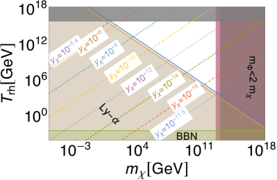
Figure 3: The white region is allowed on $(T_{\rm rh},m_{\chi})$ plane for the benchmark values ‘(m)NMP-N-1’ and ‘(m)NMP-N-2’ from Table 2 on log-log scale. The dashed or dashed-dotted lines passing through the white region correspond to Eq. 39 for different values of $y_{\chi}$ satisfying present-day CDM density. Bounds on this plane are shown as color-shaded regions, and they are coming from: Ly-$\alpha$ bound on the mass of DM Eq. 40: blue-shaded region, and $m_{\chi}\lesssim m_{\phi}/2$:copper-rose colored vertical stripe on the right for ‘(m)NM-N-1’. For ‘(m)NM-N-2’ same bounds are depicted as peach-colored region and light-copper-rose colored region. Light green-colored stripe at the bottom depicts that $T_{\rm rh}$ should be $\gtrsim 4\,\text{MeV}$. The gray colored horizontal stripe at the top of the figure indiscates that we have restricted ourselves to the highest $T_{\rm rh}$ possible in the universe to be $10^{16}\,\text{GeV}$.

This Ly-$\alpha$ bound constrains the parameter space on $(T_{\rm rh},m_{\chi})$ plane such that produced $\chi$ particles behave as CDM instead of warm dark matter (WDM) in the present universe. From the observation of Ly-$\alpha$ absorption lines, the upper bound on present-day velocity of $\chi$ particles, $v_{\chi}/c$, and lower bound $m_{\chi}$ are $v_{\chi}/c\lesssim 1.8\times 10^{-8}$ and $m_{\chi}\gtrsim 3.5\,\text{keV}$ in order to avoid being warm dark matter candidate. The maximum possible value of the initial momentum of $\chi$ particle is $m_{\phi}/2$. Then, the assumption that $\chi$ particles are feebly interacting and because of that the momentum of the particles decreases only due to the expansion of the universe, leads to the bound Bernal and Xu (2021)

$$m_{\chi}\gtrsim 2\frac{m_{\phi}}{T_{\rm rh}}\,,$$ (40)

where $m_{\chi}$ is expressed in  keV.

III.4 DM from scattering

We prefer to choose the maximum allowed value of $T_{\rm rh}$ as

$${T_{\rm rh}}_{,\text{allowable}}=\begin{cases}1.3826\times 10^{14}\,\text{GeV}\,\quad\text{(for `(m)NM-N-1')}\,,\\ 1.0637\times 10^{14}\,\text{GeV}\,\quad\text{(for `(m)NM-N-2')}\,,\\ 1.2589\times 10^{14}\,\text{GeV}\,\quad\text{(for `(m)NM-N-3')}\,,\end{cases}$$ (41)

such that $T_{max}/T_{\rm rh}>1$ is maintained. For $T_{\rm rh}\sim{T_{\rm rh}}_{,\text{allowable}}$, $T_{max}/T_{\rm rh}\sim 3.16$. Now, we explore whether DM particles generated through the scattering channels for the NM-N inflationary scenario can account fully or partially for the present-day total CDM yield or whether there exists a limit on the mass of the $\chi$-particles produced via those scattering channels such that it can only contribute completely to the total CDM density. In this study, we consider DM yield produced from three 2-to-2 scattering channels

1. $Y_{IS,0}$: yield of $\chi$ from scattering of non-relativistic inflaton with graviton as the mediator which is given by

   $$Y_{IS,0} \simeq\frac{g_{\star}^{2}}{81920g_{\star,s}}\sqrt{\frac{10}{g_{\star}}}\left(\frac{T_{\rm rh}}{M_{P}}\right)^{3}\left[\left(\frac{T_{max}}{T_{\rm rh}}\right)^{4}-1\right]\frac{m_{\chi}^{2}}{m_{\phi}^{2}}\left(1-\frac{m_{\chi}^{2}}{m_{\phi}^{2}}\right)^{3/2}\,.$$ (42)

2. $Y_{\text{SM}g,0}$: yield of $\chi$ from scattering of SM particles with graviton as mediator which is given by

   $$Y_{\text{SM}g,0} =\begin{cases}\frac{45\,\alpha_{\text{DM}}}{2\pi^{3}g_{\star,s}}\sqrt{\frac{10}{g_{\star}}}\left(\frac{T_{\rm rh}}{M_{P}}\right)^{3},\qquad\text{ for }m_{\chi}\ll T_{\rm rh}\,,\\ \frac{45\,\alpha_{\text{DM}}}{2\pi^{3}g_{\star,s}}\sqrt{\frac{10}{g_{\star}}}\frac{T_{\rm rh}^{7}}{M_{P}^{3}\,m_{\chi}^{4}}\,,\qquad\text{ for }T_{max}\gg m_{\chi}\gg T_{\rm rh}\,.\end{cases}$$ (43)

3. $Y_{\text{SM}i,0}$: yield of $\chi$ from scattering of SM particles with inflaton as mediator which is given by

   $$Y_{\text{SM}i,0} \simeq\frac{135\,y^{2}_{\chi}\,\lambda_{12}^{2}}{4\pi^{8}\,g_{\star,s}}\sqrt{\frac{10}{g_{\star}}}\,\frac{M_{P}\,T_{\rm rh}}{m_{\phi}^{4}}\,,\qquad\text{ for }T_{\rm rh}\ll m_{\phi},T_{\rm rh}>T\,.$$ (44)

The value of $\alpha_{\text{DM}}$ in Eq. 43 is $1.1\times 10^{-3}$ Bernal et al. (2018b) which depends on the coupling of gravitational interaction.

For $T_{\rm rh}\sim{T_{\rm rh}}_{,\text{allowable}}$ the condition $Y_{{\rm CDM},0}\sim Y_{IS,0}$ (from Eqs. 42 and 35) leads to the value of $m_{\chi}\sim{m_{\chi}}^{IS,0}$ as

$${m_{\chi}}^{IS,0}\sim\begin{cases}4.574\times 10^{10}\,\text{GeV}\,\quad\text{(for `(m)NM-N-1')}\,,\\ 2.8312\times 10^{10}\,\text{GeV}\,\quad\text{(for `(m)NM-N-2')}\,,\\ 4.4201\times 10^{10}\,\text{GeV}\,\quad\text{(for `(m)NM-N-3')}\,.\end{cases}$$ (45)

Hence, if $T_{\rm rh}<{T_{\rm rh}}_{,\text{allowable}}$, the value of $m_{\chi}$ should exceed the values mention in Eq. 45 in order to make the yield of DM produced through the scattering process of Eq. 42 comparable to $Y_{{\rm CDM},0}$ mentioned in Eq. 35. Hence, if $T_{\rm rh}\lesssim{T_{\rm rh}}_{,\text{allowable}}$ and $m_{\chi}\gtrsim{m_{\chi}}^{IS,0}$ for NM-N inflation, then $\chi$ produced solely through the 2-to-2 scattering of inflaton with graviton as the mediator can yield $100\%$ of the total CDM relic density.

When DM particles are produced from the scattering of SM particles via graviton mediation with $m_{\chi}\ll T_{\rm rh}$, then from Eq. 43 with $T_{\rm rh}\sim{T_{\rm rh}}_{,\text{allowable}}$,

$$Y_{\text{SM}g,0}=\begin{cases}4.3752\times 10^{-19}\,\quad\text{(for `(m)NM-N-1')}\,,\\ 1.9925\times 10^{-19}\,\quad\text{(for `(m)NM-N-2')}\,,\\ 3.3027\times 10^{-19}\,\quad\text{(for `(m)NM-N-3')}\,.\end{cases}$$ (46)

And thus to satisfy $Y_{{\rm CDM},0}$, it is required

$$m_{\chi}\gtrsim\begin{cases}9.8282\times 10^{8}\,\text{GeV}\,\quad\text{(for `(m)NM-N-1')}\,,\\ 2.1581\times 10^{9}\,\text{GeV}\,\quad\text{(for `(m)NM-N-2')}\,,\\ 1.302\times 10^{9}\,\text{GeV}\,\quad\text{(for `(m)NM-N-3')}\,.\end{cases}$$ (47)

Now, we consider production of $\chi$ only via the 2-to-2 scattering of SM particles with graviton as mediator with $T_{max}\gg m_{\chi}\gg T_{\rm rh}$. From Eq. 41, the maximum allowed value of $T_{\rm rh}\sim{\cal O}(10^{14})$ in  GeV. Furthermore, for $T_{\rm rh}\sim 10^{12}\,\text{GeV}$, $T_{max}/T_{\rm rh}\sim 30$.

However, for $(T_{max}\gg m_{\chi}\gg T_{\rm rh})$ and $Y_{\text{SM}g,0}=Y_{{\rm CDM},0}$, leads to the relation (in  GeV)

$$T_{\rm rh}^{\text{SM}g,0}=7.1389\times 10^{12}\,{f}_{T_{\rm rh}}^{-3/4}\,,$$ (48)

where ${f}_{T_{\rm rh}}=T_{\rm rh}/m_{\chi}$. Now, according to Eq. 48, in order to achieve $T_{\rm rh}\sim{\cal O}(10^{14})\,\text{GeV}$, ${f}_{T_{\rm rh}}\sim 0.03$ is required.

For the last process, 2-to-2 scattering of SM particles with inflaton as mediator with $T_{\rm rh}\ll m_{\phi}$, to make $Y_{\text{SM}i,0}\sim f_{\chi}\,Y_{{\rm CDM},0}$, where $f_{\chi}$ is the fraction of total CDM relic density that can be contributed by $Y_{\text{SM}i,0}$, we get

$${m_{\chi}}^{\text{SM}i,0}=4.2164\times 10^{-5}\frac{m_{\phi}^{4}}{T_{\rm rh}\,M_{P}\,\lambda_{12}^{2}}\,\frac{f_{c}}{y_{\chi}^{2}}\,\,\text{GeV}\,.$$ (49)

Then, with $f_{\phi}=T_{\rm rh}/m_{\phi}$ in Eq. 28 and for $y_{\chi}\sim 10^{-5}$ for all three benchmark values (‘(m)NM-N-1’, ‘(m)NM-N-2’, and ‘(m)NM-N-3’)

$$m_{\chi}\sim 3.2689\times 10^{3}\,\frac{f_{\chi}}{f_{\phi}^{3}}\,\,\text{GeV}\,.$$ (50)

For instance, with $f_{\chi}=1$ and $f_{\phi}\sim 10^{-2}$, we get $m_{\chi}\sim{\cal O}(10^{9})\,\text{GeV}$ to satisfy total CDM relic density.

Hence, three of the four scattering processes (2-to-2 scattering of non-relativistic inflaton with graviton as the mediator, 2-to-2 scattering of SM particles with graviton as mediator with $m_{\chi}\ll T_{\rm rh}$, and 2-to-2 scattering of SM particles with inflaton as mediator with $T_{\rm rh}\ll m_{\phi}$) can effectively produce $\chi$ and contribute up to $100\%$ of the total CDM relic density of the present universe in the context of NM-N inflation.

IV Periodic non-minimal coupling and natural inflation

The shift symmetry of a system is preserved if the system is invariant under a transformation of its field variables by a constant value. In natural inflation, as mentioned earlier, $\quantity(1+\cos(\varphi/f_{a}))$ is invariant under the transformation of $\varphi\to\varphi+\text{ constant}$, where the constant is $2\pi f_{a}$. In this inflationary model, we consider non-minimal coupling to gravity, which respects the same discrete shift symmetry just like the potential of natural inflation. Therefore, non-minimal coupling is specified as Ferreira et al. (2018)

$$\Omega^{2}(\varphi)=1+\alpha\left(1+\cos\left(\frac{\varphi}{f_{a}}\right)\right)\,,$$ (51)

where $\alpha$ is dimensionless. As a result of such choice of $\Omega^{2}(\varphi)$, both $\Omega^{2}(\varphi)$ and $V^{JF}(\varphi)$ possess the same shift symmetry $\varphi\to\varphi+2\pi f_{a}$. Then the potential in Einstein frame is

$$V^{E}(\phi(\varphi))\equiv V^{E}_{\rm\text{NMP-N}}(\phi(\varphi))=\frac{\Lambda^{4}\left(1+\cos\left(\frac{\varphi}{f_{a}}\right)\right)}{\quantity(1+\alpha\left(1+\cos\left(\frac{\varphi}{f_{a}}\right)\right))^{2}}$$ (52)

The periodicity of the coupling to gravity and potential is both $2\pi f_{a}$. That’s why hereafter we call this inflationary model as non-minimal periodic Natural (NMP-N) inflation. Accordingly, the part of the coupling containing $\alpha\left(1+\cos\left(\frac{\varphi}{f_{a}}\right)\right)$ vanishes at the minimum of the potential, i.e. during reheating. This particular choice ensures that reheating happens in Einstein frame. Here, in Eq. 51, $\alpha>-0.5$ is required so that Planck scale is well-defined. Furthermore, for $\alpha=0.5$, the periodicity of $V^{JF}(\varphi)$ as a function of $\varphi$ is equal to the periodicity of $V(\phi)$ as a function of $\phi$, and for $0.5<\alpha<1$, both periodicity scales are almost of the same order Ferreira et al. (2018).

$V^{E}_{\rm\text{NMP-N}}\left(\phi(\varphi)\right)$ has two sets of stationary points: (a) both at $\varphi_{a,{\rm even}}/M_{P}=2f_{a}\pi\mathbb{c}_{1}$, and at $\varphi_{a,{\rm odd}}/M_{P}=f_{a}(\pi+2\pi\mathbb{c}_{1})$, and (b) at $\varphi_{b}/M_{P}=f_{a}\,\tan^{-1}\left(\pm\frac{\sqrt{2\alpha-1}}{1-\alpha}\right)+2\pi\mathbb{c}_{1},\,\,\,\text{where}\,\mathbb{c}_{1}\in\mathbb{Z}$, set of integers. For $\alpha<0.5$, there is only one set of stationary points, i.e. $\varphi_{a,{\rm even}}$ and $\varphi_{a,{\rm odd}}$, and at those points

$$\left.\frac{\text{d}^{2}V^{E}\left(\phi(\varphi)\right)}{\text{d}\varphi^{2}}\right|_{\varphi=\varphi_{a,{\rm even}}}=\frac{(2\alpha-1){\Lambda^{4}}}{(2\alpha+1)^{3}{f_{a}}^{2}}\,,\qquad \left.\frac{\text{d}^{2}V^{E}\left(\phi(\varphi)\right)}{\text{d}\varphi^{2}}\right|_{\varphi=\varphi_{a,{\rm odd}}}=\frac{\Lambda^{4}}{f_{a}^{2}}$$ (53)

Hence, $\varphi_{a,{\rm odd}}$ is always the location of local minima, whereas, $\varphi_{a,{\rm even}}$ can be maxima or minima or saddle points depending on whether $\alpha<0.5$, or $>0.5$, or $=0.5$. In contrast, $\varphi_{b}$ is the location of maxima, or minima, or saddle points depending on whether $\alpha>0.5$, or $<0.5$, or $=0.5$. This is because

$$\left.\frac{\text{d}^{2}V^{E}\left(\phi(\varphi)\right)}{\text{d}\varphi^{2}}\right|_{\varphi=\varphi_{b}}=\frac{\quantity(1-2\alpha)\Lambda^{4}}{8\alpha\,f_{a}^{2}}\,.$$ (54)

We consider the slow roll inflationary scenario, where the inflaton begins rolling near $\varphi=0$ and continues to roll towards larger values of $\varphi$. When $\alpha<0.5$, $\varphi=0$ is the location of maximum and slow roll inflation stops whenever it becomes $\left|\eta_{V}\right|\sim 1$, and for $f_{a}\ll\alpha$, inflation may be impossible as $\left|\eta_{V}\right|>1$ even at $\varphi=0$. For $\alpha=0.5$, $\varphi=0$ is the location of saddle point and thus $\eta_{V}=\epsilon_{V}=0$ at $\varphi=0$. However, for $\alpha>0.5$ there is a maximum between $\varphi=0$ and minimum of the potential. In this case, the inflaton may travel across this maximum during its course of evolution. Our chosen benchmark values are listed in Table 4. For benchmark ‘(m)NMP-N-1’, $\varphi=0$ is a saddle point whereas For benchmark ‘(m)NMP-N-2’, there is a maximum at $\varphi/M_{P}=9\pi\approx 28.27$. The $n_{s},r$ prediction of the benchmark values are displayed in Fig. 4 along with the best-fit contours from current and future CMB observations. The predicted value of $r$ for benchmark values ‘(m)NMP-N-1’, ‘(m)NMP-N-2’, and ‘(m)NMP-N-4’ fall within $1-\sigma$ contour of Planck2018 data. Although the benchmark ‘(m)NMP-N-3’  is for ${\cal N}_{\text{CMB}}\approx 70$, the predicted value of $r$ is within $1-\sigma$ contour of Planck2018+Bicep3 (2022)+Keck Array2018 data. This benchmark value indicates that NMP-N inflation can predict values of $r$ that remain within $1-\sigma$ contour of Planck+Bicep combined data for larger e-folds. Table 4 also indicates that except for benchmark ‘(m)NMP-N-4’, which we have selected for comparison later in this section, a value of $f_{a}/M_{P}\sim{\cal O}\quantity(10-20)$ is required to predict $n_{s}\sim 0.9647$. Although these values of $f_{a}$ are slightly greater than the required value of $f_{a}$ in Table 2, these are still smaller than the value required for minimal natural inflation .

Table 4: Benchmark valuse for NMP-N inflationary model in metric formalism.

Benchmark	$f_{a}/M_{P}$	$\alpha$	$\varphi_{*}/M_{P}$	$\varphi_{\rm end}/M_{P}$	$n_{s}$	$r\times 10^{2}$	$\Lambda^{4}/M_{P}^{4}$	$\varphi_{\rm min}/M_{P}$	${\cal N}_{\text{CMB}}$
(m)NMP-N-1	$11.97$	$0.5$	$23.8164$	$36.1996$	$0.9647$	$5.043$	$4.4407\times 10^{-9}$	$37.6049$	$60$
(m)NMP-N-2	$18$	$1$	$42.4644$	$55.1417$	$0.9645$	$5.6440$	$1.0048\times 10^{-8}$	$56.5487$	$60$
(m)NMP-N-3	$6.3$	$0.48$	$8.0198$	$18.408$	$0.9651$	$0.9718$	$6.1337\times 10^{-10}$	$19.792$	$70$
(m)NMP-N-4	$164.0$	$100$	$500.831$	$513.815$	$0.9648$	$4.2071$	$6.5157\times 10^{-7}$	$515.221$	$65$

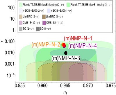
Figure 4: The colored dots represent the predicted value of $(n_{s},r)$ for two benchmark values from Table 4. Alongside, this figure also displays $68\%$ and $95\%$ C.L. $(n_{s},r)$ best-fit contour from the Planck 2018+Bicep and additional forthcoming CMB observations mentioned above in Fig. 1 .

IV.1 Reheating and production of DM from inflaton decay

The reheating scenario in this inflationary model is similar to that of NM-N inflation discussed in Sec. III.1, although the non-minimal coupling vanishes for NMP-N inflation at the minimum. The locations of the minima $\varphi_{\rm min}/M_{P}$ of the potential of Eq. 52 around which the inflaton oscillates during reheating era for the benchmark values mentioned in Table 4 and thus, the mass of the inflaton is given by Eq. 26. Following the similar approach, $\Gamma_{\varphi},T_{\rm rh}$, and ${\cal H}_{I}$ can be calculated and are listed in Table 5 for the benchmark values of Table 4. It can be observed that $m_{\phi}/M_{P}$ is almost of the same order for ‘(m)NMP-N-1’ and ‘(m)NMP-N-2’, and also for ‘(m)NMP-N-3’, ‘(m)NMP-N-4’, and hence, the same conclusion can be drawn for $T_{max}$ as ${\cal H}_{I}/M_{P}$ is almost equal for all benchmark values. For this reason, $T_{max}/T_{\rm rh}$ versus $T_{\rm rh}$ is exhibited only for ‘(m)NMP-N-1’ in Fig. 5. Gray-colored vertical stripe on the left of the plot represents the lower bound on $T_{\rm rh}\gtrsim 4\,\text{MeV}$. From Fig. 5, we get the maximum value of $T_{max}/T_{\rm rh}\sim 5.1378\times 10^{8}\,\text{GeV}$ at $T_{\rm rh}\sim 4\,\text{MeV}$ and $T_{max}/T_{\rm rh}\sim 1$ at $T_{\rm rh}\sim 1.056\times 10^{15}\,\text{GeV}$. Furthermore, lower bound on $T_{\rm rh}$ leads to establishing the minimum permissible value of $\lambda_{12}$ which are $\lambda_{12}/M_{P}\gtrsim 4.4662\times 10^{-23}$ for ‘(m)NMP-N-1’, $\lambda_{12}/M_{P}\gtrsim 4.4669\times 10^{-23}$ for ‘(m)NMP-N-2’, $\lambda_{12}/M_{P}\gtrsim 3.753\times 10^{-23}$ for ‘(m)NMP-N-3’, and $\lambda_{12}/M_{P}\gtrsim 4.1994\times 10^{-23}$ for ‘(m)NMP-N-4’.

Table 5: $m_{\varphi},\Gamma_{\varphi},T_{\rm rh}$, and ${\cal H}_{I}$ for the benchmark values from Table 4.

Benchmark	$m_{\phi}/M_{P}$	$\Gamma_{\phi}M_{P}$	$T_{\rm rh}/\lambda_{12}$	${\cal H}_{I}/M_{P}$
	(Eq. (26))	(Eq. (24))	(Eq. (28))	(Eq. 29)
(m)NMP-N-1	$5.5671\times 10^{-6}$	$7147.08\,\lambda_{12}^{2}$	$37.3175$	$3.1881\times 10^{-6}$
(m)NMP-N-2	$5.5689\times 10^{-6}$	$7144.85\,\lambda_{12}^{2}$	$37.3117$	$3.1882\times 10^{-6}$
(m)NMP-N-3	$3.9312\times 10^{-6}$	$10121.40\,\lambda_{12}^{2}$	$44.4087$	$2.1915\times 10^{-6}$
(m)NMP-N-4	$4.9219\times 10^{-6}$	$8083.95\,\lambda_{12}^{2}$	$39.6881$	$2.8152\times 10^{-6}$

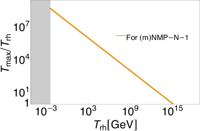
Figure 5: Variation of $T_{max}/T_{\rm rh}$ against $T_{\rm rh}$ for benchmark value ‘(m)NMP-N-1’ from Table 4. The gray-colored vertical stripe on the left of the plot of lower bound on $T_{\rm rh}$ which is $T_{\rm rh}\nless 4\,\text{MeV}$.

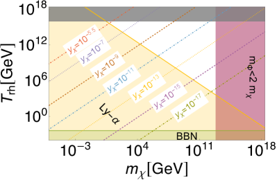
Figure 6: The white region is allowed on $(T_{\rm rh},m_{\chi})$ plane for the benchmark value ‘(m)NMP-N-1’from Table 4 on log-log scale. The dashed or dashed-dotted lines passing through the white region correspond to Eq. 39 for different values of $y_{\chi}$ satisfying present-day CDM density. Bounds on this plane are shown as color-shaded regions, and they are coming from: Ly-$\alpha$ bound on the mass of DM (Eq. 40): peach-colored region, and $m_{\chi}\lesssim m_{\phi}/2$: copper-rose colored vertical stripe on the right. Light green-colored stripe at the bottom depicts that $T_{\rm rh}$ should be $\gtrsim 4\,\text{MeV}$. The horizontal stripe at the top highlighted in gray is for $T_{\rm rh}\lesssim 10^{16}\,\text{GeV}$.

Similar to Fig. 3, the discontinuous and inclined lines visible on $(T_{\rm rh},m_{\chi})$ plane in Fig. 6 correspond to $\chi$ producing from the decay of inflaton during reheating in NMP-N inflation which can completely account for the total CDM density as stated by Eq. 39. The bounds on this plane are for Ly-$\alpha$ from Eq. 40 (peach-shaded region), from BBN temperature (green-colored horizontal stripe at the bottom), $m_{\chi}\lesssim m_{\phi}/2$ (copper-rose colored vertical stripe at the right of the plot), and horizontal stripe at the top highlighted in gray for our assumption that the upper limit for $T_{\rm rh}$ is $\sim 10^{16}\,\text{GeV}$. The upper and lower bound of $y_{\chi}$ are $\lesssim{\cal O}(10^{-7})$ and $\gtrsim{\cal O}(10^{-17})$ (for $2.67\,\text{GeV}m_{\chi}\lesssim 6.68\times 10^{12}\,\text{GeV}$) to account for the total CDM yield, produced through decay channel. Since the allowed region on $(T_{\rm rh},m_{\chi})$ plane for NMP-N inflation varies for all the chosen benchmark values, similar to the scenario explicitly displayed in Fig. 3 of NM-N inflation, it is expected that ranges of $y_{\chi}$ and $m_{\chi}$ will not be exactly identical for all the benchmark values from Table 4.

IV.2 DM from scattering

Similar to Eq. 41 in NM-N inflationary scenario, we can define ${T_{\rm rh}}_{,\text{allowable}}$ for NMP-N inflationary scenario such that $T_{max}/{T_{\rm rh}}_{,\text{allowable}}\sim 3.16$ as

$${T_{\rm rh}}_{,\text{allowed}}=\begin{cases}1.0559\times 10^{14}\,\text{GeV}\,\quad\text{(for `(m)NMP-N-1')}\,,\\ 1.0571\times 10^{14}\,\text{GeV}\,\quad\text{(for `(m)NMP-N-2')}\,,\\ 8.7639\times 10^{13}\,\text{GeV}\,\quad\text{(for `(m)NMP-N-3')}\,,\\ 9.9331\times 10^{13}\,\text{GeV}\,\quad\text{(for `(m)NMP-N-4')}\,.\end{cases}$$ (55)

Now, for $T_{\rm rh}\lesssim{T_{\rm rh}}_{,\text{ allowable}}$, the condition for $Y_{{\rm CDM},0}\sim Y_{IS,0}$ (from Eqs. 35 and 42) leads to $m_{\chi}\sim{m_{\chi}}^{IS,0}$ such that

$${m_{\chi}}^{IS,0}\sim\begin{cases}2.8369\times 10^{10}\,\text{GeV}\,\quad\text{(for `(m)NMP-N-1')}\,,\\ 2.8343\times 10^{10}\,\text{GeV}\,\quad\text{(for `(m)NMP-N-2')}\,,\\ 2.7103\times 10^{10}\,\text{GeV}\,\quad\text{(for `(m)NMP-N-3')}\,,\\ 2.7778\times 10^{10}\,\text{GeV}\,\quad\text{(for `(m)NMP-N-4')}\,.\end{cases}$$ (56)

Therefore, if $T_{\rm rh}<{T_{\rm rh}}_{,\text{allowable}}$, the value of $m_{\chi}$ should exceed the values mention in Eq. 56 in order to make the yield of DM produced through the scattering process of Eq. 42 comparable to $Y_{{\rm CDM},0}$ mentioned in Eq. 35. Hence, if $T_{\rm rh}\lesssim{T_{\rm rh}}_{,\text{allowed}}$ and $m_{\chi}\gtrsim{m_{\chi}}_{,1}$ for NM-N inflation, then $\chi$ produced solely through the 2-to-2 scattering of inflaton with graviton as the mediator can yield $100\%$ of the total CDM relic density.

When DM particles are produced from the scattering of SM particles via graviton mediation (Eq. 43 with $m_{\chi}\ll T_{\rm rh}$ and $T_{\rm rh}\sim{T_{\rm rh}}_{,\text{allowable}}$)

$$Y_{\text{SM}g,0}=\begin{cases}1.9489\times 10^{-19}\,\text{GeV}\,\quad\text{(for `(m)NMP-N-1')}\,,\\ 1.9554\times 10^{-19}\,\text{GeV}\,\quad\text{(for `(m)NMP-N-2')}\,,\\ 1.1144\times 10^{-19}\,\text{GeV}\,\quad\text{(for `(m)NMP-N-3')}\,,\\ 1.6225\times 10^{-19}\,\text{GeV}\,\quad\text{(for `(m)NMP-N-4')}\,.\end{cases}$$ (57)

And thus to satisfy $Y_{{\rm CDM},0}$, it is required

$$m_{\chi}\sim\begin{cases}2.2064\times 10^{9}\,\text{GeV}\,\quad\text{(for `(m)NMP-N-1')}\,,\\ 2.1990\times 10^{9}\,\text{GeV}\,\quad\text{(for `(m)NMP-N-2')}\,,\\ 3.8586\times 10^{9}\,\text{GeV}\,\quad\text{(for `(m)NMP-N-3')}\,,\\ 2.6502\times 10^{9}\,\text{GeV}\,\quad\text{(for `(m)NMP-N-4')}\,.\end{cases}$$ (58)

However, since ${T_{\rm rh}}_{,\text{ allowable}}\sim{\cal O}(10^{14})\,\text{GeV}$ (see Eq. 55) similar to NM-N inflation, the conclusion remains the same as that of NM-N, for the production of $\chi$ via 2-to-2 scattering of SM particles with graviton as mediator with $T_{max}\gg m_{\chi}\gg T_{\rm rh}$ process.

For the last scattering process (2-to-2 scattering of SM particles with inflaton as mediator with $T_{\rm rh}\ll m_{\phi}$), for $Y_{\text{SM}i,0}\sim f_{\chi}\,Y_{{\rm CDM},0}$, and from Eq. 49 with $y_{\chi}\sim 10^{-5}$ we again get for the four benchmark values

$$m_{\chi}\sim 3.2689\times 10^{3}\,\frac{f_{\chi}}{f_{\phi}^{3}}\,\text{GeV}$$ (59)

If we take $f_{\chi}=1$ and $f_{\phi}\sim 10^{-2}$, we can obtain $m_{\chi}\sim{\cal O}(10^{9})\,\text{GeV}$ to satisfy the total CDM relic density.

V Discussion and Conclusion

In this work, we studied single-field natural inflation model with non-minimal coupling between the inflaton and the gravity sector. Two forms of non-minimal coupling - $\xi\varphi^{2}{\cal R}$ and $\alpha\left(1+\cos\left(\frac{\varphi}{f_{a}}\right)\right)$ were factored in. For both the inflationary scenarios, considering CMB bounds, we explored the parameter space of $y_{\chi}$, $m_{\chi}$, and $\lambda_{12}$, for the production of a fermionic DM particle $\chi$ during post-inflationary reheating era, as a potential candidate for the CDM of the present universe. Key findings of this investigation are summarized below:

• We found that NMP-N inflationary scenario requires a slightly larger value for $f_{a}/M_{P}$ ($f_{a}/M_{P}\sim{\cal O}(10)$) compared to NM-N inflationary scenario ($f_{a}/M_{P}\sim{\cal O}(1)$) to satisfy bounds from CMB measurements (see Tables 2 and 4). However, both models predict values of $r\sim 1.7231\times 10^{-2}$ for NM-N, and $r\sim 9.7184\times 10^{-3}$ for NMP-N which fall within $1-\sigma$ contour of joint analysis of Planck2018+Bicep3 (2022)+Keck Array2018 but for ${\cal N}_{\text{CMB}}>60$. These values of $r$ can be verified in future by upcoming CMB observations, e.g. SO.

• From Tables 3 and 5, we conclude that the value of $m_{\phi}$ varies depending on benchmarks for both inflationary scenarios, being highest ($\sim 4.0987\times 10^{13}\,\text{GeV}$) for ‘(m)NM-N-1’ and lowest for ‘(m)NMP-N-3’ ($\sim 9.4349\times 10^{12}\,\text{GeV}$), consequently affecting $T_{\rm rh}$, Ly-$\alpha$ bound and maximum possible value of $m_{\chi}$. However, unlike NM-N inflationary scenario, the value of ${\cal H}_{I}$ remains nearly the same for various benchmark values ($f_{a}/M_{P}$ was varied from $6.3$ to $164.0$) for NMP-N inflation due to the vanishing of non-minimal coupling near the minimum.

• Variation of $T_{max}/T_{\rm rh}$ against $T_{\rm rh}$ for different benchmarks for NM-N and NMP-N inflation are shown in Figs. 2 and 5. $T_{max}/T_{\rm rh}$ is the highest $(\sim{\cal O}\quantity(10^{8}))$ at $T_{\rm rh}\sim 4\,\text{MeV}$, e.g. $T_{max}/T_{\rm rh}\sim 5.88\times 10^{8}$ for ‘(m)NM-N-1’and $T_{max}/T_{\rm rh}\sim 5.14\times 10^{8}$ for ‘(m)NMP-N-1’. Hence, inflationary parameters, including $\Lambda$, $f_{a}$ and $r$, controls $T_{max}/T_{\rm rh}$.

• From Figs. 3 and 6 we conclude that $\chi$ produced only through inflaton decay can contributes $100\%$ of the total relic density of CDM of the present universe if the allowed range of $y_{\chi}$ is $10^{-6}\gtrsim y_{\chi}\gtrsim 10^{-17}$ and of $m_{\chi}$ is ${\cal O}(1\,\text{GeV})\lesssim m_{\chi}\lesssim m_{\phi}/2$ for NM-N and NMP-N inflationary scenarios. The exact range of $y_{\chi}$ and $m_{\chi}$, however, varies depending on our assumed maximum value of $T_{\rm rh}$ and benchmark values (for example, see Fig. 3), and thus for different values of inflationary parameters and also for different inflationary scenarios.

• If we assume that $\chi$ is produced only via scattering of non-relativistic inflaton with graviton as the mediator or via scattering of SM particles with graviton as a mediator with $m_{\chi}\ll T_{\rm rh}$, then the DM produced through those scattering channels separately for all chosen benchmark values and inflationary scenarios can make $100\%$ of the total CDM yield of the present universe, provided $m_{\chi}\gtrsim{\cal O}(10^{10})\,\text{GeV}$ (see Eqs. 45 and 56) and $m_{\chi}\gtrsim{\cal O}(10^{9})\,\text{GeV}$ (see Eqs. 47 and 58), respectively. However, the exact value of $m_{\chi}$ varies depending on the benchmark as well as the inflationary scenario being considered. However, scattering channel of SM particles with graviton as mediator with $T_{max}\gg m_{\chi}\gg T_{\rm rh}$ seems less effective to produce the total CDM relic density. Furthermore, for scattering of SM particles with inflaton as mediator $m_{\chi}\sim{\cal O}(10^{9})\,\text{GeV}$ (Eqs. 50 and 59), for example, is required for $T_{\rm rh}\sim 10^{-3}m_{\phi}$ and $y_{\chi}\sim 10^{-5}$ to contribute completely to the total CDM density.

In this paper, just by extending the standard model with two degrees of freedom: an axion-like particle (inflaton), and a fermionic DM, we demonstrated how to obtain the tiny temperature fluctuations as seen in the CMB as well as address the DM puzzle of the universe in terms of its possible particle origin. We showed how future measurements of the CMB from experiments like CMB-S4, LiteBIRD, and SO Abazajian et al. (2022); Allys et al. (2023); Ade et al. (2019) and other such experiments Hazumi et al. (2019); Adak et al. (2022); Sayre et al. (2020); Suzuki et al. (2016); Aiola et al. (2020); Harrington et al. (2016); Addamo et al. (2021); Mennella et al. (2019); Ade et al. (2022b) will further be able to verify the simple models we have presented if BB-modes are detected and the scale of inflation is measured. The presence of interaction with inflaton and DM species may lead to non-Gaussianities and may serve as very interesting probes of these models and complementary signatures of non-thermal production of DM. But such a study is beyond the scope of the present draft and will be taken up in future publications.

References

- Starobinsky (1980) A. A. Starobinsky, Phys. Lett. B 91, 99 (1980).
- Guth (1981) A. H. Guth, Phys. Rev. D 23, 347 (1981).
- Linde (1982) A. D. Linde, Phys. Lett. B 108, 389 (1982).
- Albrecht and Steinhardt (1982) A. Albrecht and P. J. Steinhardt, Phys. Rev. Lett. 48, 1220 (1982).
- Akrami et al. (2020) Y. Akrami et al. (Planck), Astron. Astrophys. 641, A10 (2020), arXiv:1807.06211 [astro-ph.CO] .
- Ade et al. (2018) P. A. R. Ade et al. (BICEP2, Keck Array), Phys. Rev. Lett. 121, 221301 (2018), arXiv:1810.05216 [astro-ph.CO] .
- Folkerts et al. (2014) S. Folkerts, C. Germani, and J. Redondo, Phys. Lett. B 728, 532 (2014), arXiv:1304.7270 [hep-ph] .
- Martin et al. (2014) J. Martin, C. Ringeval, and V. Vennin, Phys. Dark Univ. 5-6, 75 (2014), arXiv:1303.3787 [astro-ph.CO] .
- Hertzberg (2010) M. P. Hertzberg, JHEP 11, 023 (2010), arXiv:1002.2995 [hep-ph] .
- Bertone et al. (2005) G. Bertone, D. Hooper, and J. Silk, Phys. Rept. 405, 279 (2005), arXiv:hep-ph/0404175 .
- Bernal et al. (2018a) N. Bernal, A. Chatterjee, and A. Paul, JCAP 12, 020 (2018a), arXiv:1809.02338 [hep-ph] .
- McDonald (2002) J. McDonald, Phys. Rev. Lett. 88, 091304 (2002), arXiv:hep-ph/0106249 .
- Choi and Roszkowski (2005) K.-Y. Choi and L. Roszkowski, AIP Conf. Proc. 805, 30 (2005), arXiv:hep-ph/0511003 .
- Kusenko (2006) A. Kusenko, Phys. Rev. Lett. 97, 241301 (2006), arXiv:hep-ph/0609081 .
- Petraki and Kusenko (2008) K. Petraki and A. Kusenko, Phys. Rev. D 77, 065014 (2008), arXiv:0711.4646 [hep-ph] .
- Hall et al. (2010) L. J. Hall, K. Jedamzik, J. March-Russell, and S. M. West, JHEP 03, 080 (2010), arXiv:0911.1120 [hep-ph] .
- Bernal et al. (2017) N. Bernal, M. Heikinheimo, T. Tenkanen, K. Tuominen, and V. Vaskonen, Int. J. Mod. Phys. A 32, 1730023 (2017), arXiv:1706.07442 [hep-ph] .
- Baer et al. (2015) H. Baer, K.-Y. Choi, J. E. Kim, and L. Roszkowski, Phys. Rept. 555, 1 (2015), arXiv:1407.0017 [hep-ph] .
- Garny et al. (2016) M. Garny, M. Sandora, and M. S. Sloth, Phys. Rev. Lett. 116, 101302 (2016), arXiv:1511.03278 [hep-ph] .
- Tang and Wu (2016) Y. Tang and Y.-L. Wu, Phys. Lett. B 758, 402 (2016), arXiv:1604.04701 [hep-ph] .
- Tang and Wu (2017) Y. Tang and Y.-L. Wu, Phys. Lett. B 774, 676 (2017), arXiv:1708.05138 [hep-ph] .
- Garny et al. (2018) M. Garny, A. Palessandro, M. Sandora, and M. S. Sloth, JCAP 02, 027 (2018), arXiv:1709.09688 [hep-ph] .
- Bernal et al. (2018b) N. Bernal, M. Dutra, Y. Mambrini, K. Olive, M. Peloso, and M. Pierre, Phys. Rev. D 97, 115020 (2018b), arXiv:1803.01866 [hep-ph] .
- Barman et al. (2023) B. Barman, A. Ghoshal, B. Grzadkowski, and A. Socha, (2023), arXiv:2305.00027 [hep-ph] .
- Barman et al. (2022a) B. Barman, P. S. Bhupal Dev, and A. Ghoshal, (2022a), arXiv:2210.07739 [hep-ph] .
- Barman and Ghoshal (2022a) B. Barman and A. Ghoshal, JCAP 10, 082 (2022a), arXiv:2203.13269 [hep-ph] .
- Barman et al. (2022b) B. Barman, P. Ghosh, A. Ghoshal, and L. Mukherjee, JCAP 08, 049 (2022b), arXiv:2112.12798 [hep-ph] .
- Barman and Ghoshal (2022b) B. Barman and A. Ghoshal, JCAP 03, 003 (2022b), arXiv:2109.03259 [hep-ph] .
- Ghosh et al. (2023) D. K. Ghosh, A. Ghoshal, and S. Jeesun, (2023), arXiv:2305.09188 [hep-ph] .
- Ghoshal et al. (2022a) A. Ghoshal, L. Heurtier, and A. Paul, JHEP 12, 105 (2022a), arXiv:2208.01670 [hep-ph] .
- Berbig and Ghoshal (2023) M. Berbig and A. Ghoshal, JHEP 05, 172 (2023), arXiv:2301.05672 [hep-ph] .
- Paul et al. (2019) A. Paul, A. Ghoshal, A. Chatterjee, and S. Pal, Eur. Phys. J. C 79, 818 (2019), arXiv:1808.09706 [astro-ph.CO] .
- Ghoshal and Saha (2022) A. Ghoshal and P. Saha, (2022), arXiv:2203.14424 [hep-ph] .
- (34) A. Ghoshal, M. Y. Khlopov, Z. Lalak, and S. Porey, draft in preparation 2306.XXXXX .
- Nozari and Sadatian (2008) K. Nozari and S. D. Sadatian, Mod. Phys. Lett. A 23, 2933 (2008), arXiv:0710.0058 [astro-ph] .
- Cheong et al. (2022) D. Y. Cheong, S. M. Lee, and S. C. Park, JCAP 02, 029 (2022), arXiv:2111.00825 [hep-ph] .
- Kodama and Takahashi (2022) T. Kodama and T. Takahashi, Phys. Rev. D 105, 063542 (2022), arXiv:2112.05283 [astro-ph.CO] .
- Shaposhnikov et al. (2020) M. Shaposhnikov, A. Shkerin, and S. Zell, JCAP 07, 064 (2020), arXiv:2002.07105 [hep-ph] .
- Oda et al. (2018) S. Oda, N. Okada, D. Raut, and D.-s. Takahashi, Phys. Rev. D 97, 055001 (2018), arXiv:1711.09850 [hep-ph] .
- Järv et al. (2017) L. Järv, K. Kannike, L. Marzola, A. Racioppi, M. Raidal, M. Rünkla, M. Saal, and H. Veermäe, Phys. Rev. Lett. 118, 151302 (2017), arXiv:1612.06863 [hep-ph] .
- Lyth (1993) D. H. Lyth, in Summer School in High-energy Physics and Cosmology (Includes Workshop on Strings, Gravity, and Related Topics 29-30 Jul 1993) (1993) pp. 0069–136, arXiv:astro-ph/9312022 .
- Baumann (2022) D. Baumann, Cosmology (Cambridge University Press, 2022).
- Bambi and Dolgov (2015) C. Bambi and A. D. Dolgov, Introduction to Particle Cosmology, UNITEXT for Physics (Springer, 2015).
- Aghanim et al. (2020) N. Aghanim et al. (Planck), Astron. Astrophys. 641, A6 (2020), [Erratum: Astron.Astrophys. 652, C4 (2021)], arXiv:1807.06209 [astro-ph.CO] .
- Workman et al. (2022) R. L. Workman et al. (Particle Data Group), PTEP 2022, 083C01 (2022).
- Ade et al. (2022a) P. A. R. Ade et al. (BICEP/Keck), in 56th Rencontres de Moriond on Cosmology (2022) arXiv:2203.16556 [astro-ph.CO] .
- Ade et al. (2021) P. A. R. Ade et al. (BICEP, Keck), Phys. Rev. Lett. 127, 151301 (2021), arXiv:2110.00483 [astro-ph.CO] .
- Campeti and Komatsu (2022) P. Campeti and E. Komatsu, Astrophys. J. 941, 110 (2022), arXiv:2205.05617 [astro-ph.CO] .
- Bernal and Xu (2021) N. Bernal and Y. Xu, Eur. Phys. J. C 81, 877 (2021), arXiv:2106.03950 [hep-ph] .
- Ghoshal et al. (2022b) A. Ghoshal, G. Lambiase, S. Pal, A. Paul, and S. Porey, JHEP 09, 231 (2022b), arXiv:2206.10648 [hep-ph] .
- Ghoshal et al. (2023a) A. Ghoshal, G. Lambiase, S. Pal, A. Paul, and S. Porey, Symmetry 15, 543 (2023a).
- Ghoshal et al. (2022c) A. Ghoshal, G. Lambiase, S. Pal, A. Paul, and S. Porey, in 25th Workshop on What Comes Beyond the Standard Models? (2022) arXiv:2211.15061 [astro-ph.CO] .
- Ghoshal et al. (2023b) A. Ghoshal, Z. Lalak, and S. Porey, (2023b), arXiv:2302.03268 [hep-ph] .
- Peccei (2008) R. D. Peccei, Lect. Notes Phys. 741, 3 (2008), arXiv:hep-ph/0607268 .
- Hook (2019) A. Hook, PoS TASI2018, 004 (2019), arXiv:1812.02669 [hep-ph] .
- Kim and Carosi (2010) J. E. Kim and G. Carosi, Rev. Mod. Phys. 82, 557 (2010), [Erratum: Rev.Mod.Phys. 91, 049902 (2019)], arXiv:0807.3125 [hep-ph] .
- Kim et al. (2005) J. E. Kim, H. P. Nilles, and M. Peloso, JCAP 01, 005 (2005), arXiv:hep-ph/0409138 .
- Freese et al. (1990) K. Freese, J. A. Frieman, and A. V. Olinto, Phys. Rev. Lett. 65, 3233 (1990).
- Savage et al. (2006) C. Savage, K. Freese, and W. H. Kinney, Phys. Rev. D 74, 123511 (2006), arXiv:hep-ph/0609144 .
- Cheng et al. (2021) W. Cheng, L. Bian, and Y.-F. Zhou, Phys. Rev. D 104, 063010 (2021), arXiv:2104.06602 [hep-ph] .
- Daido et al. (2017) R. Daido, F. Takahashi, and W. Yin, JCAP 05, 044 (2017), arXiv:1702.03284 [hep-ph] .
- Reyimuaji and Zhang (2021) Y. Reyimuaji and X. Zhang, JCAP 03, 059 (2021), arXiv:2012.14248 [astro-ph.CO] .
- Birrell and Davies (1984) N. D. Birrell and P. C. W. Davies, Quantum Fields in Curved Space, Cambridge Monographs on Mathematical Physics (Cambridge Univ. Press, Cambridge, UK, 1984).
- Faraoni (1996) V. Faraoni, Phys. Rev. D 53, 6813 (1996), arXiv:astro-ph/9602111 .
- Hrycyna (2017) O. Hrycyna, Phys. Lett. B 768, 218 (2017), arXiv:1511.08736 [astro-ph.CO] .
- Hazumi et al. (2020) M. Hazumi et al. (LiteBIRD), Proc. SPIE Int. Soc. Opt. Eng. 11443, 114432F (2020), arXiv:2101.12449 [astro-ph.IM] .
- Abazajian et al. (2016) K. N. Abazajian et al. (CMB-S4), (2016), arXiv:1610.02743 [astro-ph.CO] .
- Ade et al. (2019) P. Ade et al. (Simons Observatory), JCAP 02, 056 (2019), arXiv:1808.07445 [astro-ph.CO] .
- Enqvist (2012) K. Enqvist, in 2010 European School of High Energy Physics (2012) arXiv:1201.6164 [gr-qc] .
- Garcia et al. (2020) M. A. G. Garcia, K. Kaneta, Y. Mambrini, and K. A. Olive, Phys. Rev. D 101, 123507 (2020), arXiv:2004.08404 [hep-ph] .
- Watanabe and Komatsu (2007) Y. Watanabe and E. Komatsu, Phys. Rev. D 75, 061301 (2007), arXiv:gr-qc/0612120 .
- Kannike et al. (2017) K. Kannike, A. Racioppi, and M. Raidal, Nucl. Phys. B 918, 162 (2017), arXiv:1605.09378 [hep-ph] .
- Babichev et al. (2020) E. Babichev, D. Gorbunov, S. Ramazanov, and L. Reverberi, JCAP 09, 059 (2020), arXiv:2006.02225 [hep-ph] .
- Cembranos et al. (2020) J. A. R. Cembranos, L. J. Garay, and J. M. Sánchez Velázquez, JHEP 06, 084 (2020), arXiv:1910.13937 [hep-ph] .
- Kolb et al. (2003) E. W. Kolb, A. Notari, and A. Riotto, Phys. Rev. D 68, 123505 (2003), arXiv:hep-ph/0307241 .
- Giudice et al. (2001) G. F. Giudice, E. W. Kolb, and A. Riotto, Phys. Rev. D 64, 023508 (2001), arXiv:hep-ph/0005123 .
- Chung et al. (1999) D. J. H. Chung, E. W. Kolb, and A. Riotto, Phys. Rev. D 60, 063504 (1999), arXiv:hep-ph/9809453 .
- Drewes et al. (2017) M. Drewes, J. U. Kang, and U. R. Mun, JHEP 11, 072 (2017), arXiv:1708.01197 [astro-ph.CO] .
- Drewes (2022) M. Drewes, JCAP 09, 069 (2022), arXiv:1903.09599 [astro-ph.CO] .
- Hasegawa et al. (2019) T. Hasegawa, N. Hiroshima, K. Kohri, R. S. L. Hansen, T. Tram, and S. Hannestad, JCAP 12, 012 (2019), arXiv:1908.10189 [hep-ph] .
- Kawasaki et al. (1999) M. Kawasaki, K. Kohri, and N. Sugiyama, Phys. Rev. Lett. 82, 4168 (1999), arXiv:astro-ph/9811437 .
- Kawasaki et al. (2000) M. Kawasaki, K. Kohri, and N. Sugiyama, Phys. Rev. D 62, 023506 (2000), arXiv:astro-ph/0002127 .
- Ferreira et al. (2018) R. Z. Ferreira, A. Notari, and G. Simeon, JCAP 11, 021 (2018), arXiv:1806.05511 [astro-ph.CO] .
- Abazajian et al. (2022) K. Abazajian et al. (CMB-S4), Astrophys. J. 926, 54 (2022), arXiv:2008.12619 [astro-ph.CO] .
- Allys et al. (2023) E. Allys et al. (LiteBIRD), PTEP 2023, 042F01 (2023), arXiv:2202.02773 [astro-ph.IM] .
- Hazumi et al. (2019) M. Hazumi et al., J. Low Temp. Phys. 194, 443 (2019).
- Adak et al. (2022) D. Adak, A. Sen, S. Basak, J. Delabrouille, T. Ghosh, A. Rotti, G. Martínez-Solaeche, and T. Souradeep, Mon. Not. Roy. Astron. Soc. 514, 3002 (2022), arXiv:2110.12362 [astro-ph.CO] .
- Sayre et al. (2020) J. T. Sayre et al. (SPT), Phys. Rev. D 101, 122003 (2020), arXiv:1910.05748 [astro-ph.CO] .
- Suzuki et al. (2016) A. Suzuki et al. (POLARBEAR), J. Low Temp. Phys. 184, 805 (2016), arXiv:1512.07299 [astro-ph.IM] .
- Aiola et al. (2020) S. Aiola et al. (ACT), JCAP 12, 047 (2020), arXiv:2007.07288 [astro-ph.CO] .
- Harrington et al. (2016) K. Harrington et al., Proc. SPIE Int. Soc. Opt. Eng. 9914, 99141K (2016), arXiv:1608.08234 [astro-ph.IM] .
- Addamo et al. (2021) G. Addamo et al. (LSPE), JCAP 08, 008 (2021), arXiv:2008.11049 [astro-ph.IM] .
- Mennella et al. (2019) A. Mennella et al., Universe 5, 42 (2019).
- Ade et al. (2022b) P. A. R. Ade et al. (SPIDER), Astrophys. J. 927, 174 (2022b), arXiv:2103.13334 [astro-ph.CO] .