Densities and mass assembly histories of the Milky Way satellites
are not a challenge to CDM
Abstract
We use the GRUMPY galaxy formation model based on a suite of zoom-in, high-resolution, dissipationless CDM simulations of the Milky Way (MW) sized haloes to examine total matter density within the half-mass radius of stellar distribution, , of satellite dwarf galaxies around the MW hosts and their mass assembly histories. We compare model results to estimates for observed dwarf satellites of the Milky Way spanning their entire luminosity range. We show that observed MW dwarf satellites exhibit a trend of decreasing total matter density within a half-mass radius, , with increasing stellar mass. This trend is in general agreement with the trend predicted by the model. None of the observed satellites are overly dense compared to the results of our CDM-based model. We also show that although the halo mass of many satellite galaxies is comparable to the halo mass of the MW progenitor at , at these early epochs halos that survive as satellites to are located many virial radii away from the MW progenitors and thus do not have a chance to merge with it. Our results show that neither the densities estimated in observed Milky Way satellites nor their mass assembly histories pose a challenge to the CDM model. In fact, the broad agreement between density trends with the stellar mass of the observed and model galaxies can be considered as yet another success of the model.
keywords:
galaxies: evolution, galaxies: formation, galaxies: dwarf, galaxies: haloes1 Introduction
Dwarf galaxies orbiting around the Milky Way allow us to study galaxy formation and test Cold Dark Matter model (hereafter CDM) at the smallest scales (see, e.g., Read et al., 2016; Bullock & Boylan-Kolchin, 2017; Sales et al., 2022, for reviews). In particular, total matter density estimates in the inner regions of dwarf galaxies are used as one of the key tests of CDM model (e.g., Boylan-Kolchin et al., 2011; Oh et al., 2015; Read et al., 2016) and can be used to distinguish between models in which dark matter has different degrees of self-interaction (e.g., Silverman et al., 2023).
Safarzadeh & Loeb (2021) recently used density within half-light radius estimated for a sample of observed nearby dwarf galaxies and some additional model assumptions to estimate the formation epoch of their parent haloes and their mass at that epoch. They argued that some of the dwarf galaxies with the largest densities have masses at that are comparable to the expected mass of the Milky Way (hereafter MW) progenitor and that this fact is a challenge to the CDM model.
In this study, we examine this challenge in detail. We use a suite of high-resolution Caterpillar simulations of MW-sized halos (Griffen et al., 2016) and a model of dwarf galaxy formation of Kravtsov & Manwadkar (2022) to model the evolution of the MW satellites and their observable properties, such as -band luminosities and half-mass radii, . The model predicts the total mass density within , , and we compare the predicted densities with the estimates for observed MW satellites. For the latter, we use an up-to-date compilation of half-light radii, luminosities, and stellar velocity measurements for the entire range of stellar masses of the observed MW satellites and the dynamical mass estimator of Wolf et al. (2010).
We find that of observed satellites decreases with increasing stellar mass and this relation is reproduced by the model. There is thus no discrepancy between of the MW satellites and predicted densities of satellites in the CDM model. Likewise, we find that the masses of some of the surviving MW satellites have likely been comparable to the MW mass at . However, this is not an issue because at that time these satellites were far from the main MW progenitor and this is why they did not merge with it.
2 Modelling Milky Way satellite system
We model the population of Milky Way dwarf satellite galaxies around the Milky Way using tracks of haloes and subhaloes from the Caterpillar (Griffen et al., 2016) suite of -body simulations111https://www.caterpillarproject.org of 32 MW-sized haloes. We use the highest resolution suite LX14 to maximize the dynamic range of halo masses probed by our modelling.
The haloes were identified using the modified version of the Rockstar halo finder and the Consistent Trees Code (Behroozi et al., 2013), with modification improving recovery of the subhaloes with high fraction of unbound particles (see discussion in Section 2.5 of Griffen et al., 2016). As was shown in Manwadkar & Kravtsov (2022) (see their Fig. 1), the subhalo peak mass function in the LX14 simulations is complete at , or for the host halo mass , even in the innermost regions of the host ( kpc). This is sufficient to model the full range of luminosities of observed Milky Way satellites, as faintest ultrafaint dwarfs are hosted in haloes of in our model (Kravtsov & Manwadkar, 2022; Manwadkar & Kravtsov, 2022). Moreover, in this study we use only galaxies hosted in haloes with .
The mass evolution tracks of subhaloes of MW-sized host haloes are used as input for the GRUMPY galaxy formation model, which evolves various properties of gas and stars of the galaxies they host. As a regulator-type galaxy formation framework (e.g., Krumholz & Dekel, 2012; Lilly et al., 2013; Feldmann, 2013), GRUMPY is designed to model galaxies of luminosity (Kravtsov & Manwadkar, 2022), which follows the evolution of a number of key galaxy properties by solving a system of coupled differential equations. The model accounts for UV heating after reionization and associated gas accretion suppression onto small mass haloes, galactic outflows, a model for gaseous disk and its size, molecular hydrogen mass, star formation, etc. The evolution of the half-mass radius of the stellar distribution is also modelled. The galaxy model parameters used in this study are identical to those used in Manwadkar & Kravtsov (2022).
Here we use the model to predict luminosities, stellar masses, and stellar half-mass radii (sizes) of satellite galaxies around the MW-sized haloes from the Caterpillar suite. To estimate luminosity in the -band filter we use the Flexible Stellar Population Synthesis (FSPS) code (Conroy et al., 2009; Conroy & Gunn, 2010) in conjunction with its Python bindings, PyFSPS 222https://github.com/dfm/python-fsps and star formation histories and metallicity evolution of the model galaxies.
The GRUMPY model is described and tested against a wide range of observations of local dwarf galaxies in Kravtsov & Manwadkar (2022). Importantly for this study, the model was shown to reproduce luminosity function and radial distribution of the Milky Way satellites and size-luminosity relation of observed dwarf galaxies (Manwadkar & Kravtsov, 2022). We thus use luminosities of model galaxies to select counterparts of observed MW satellites, while half-mass radii are used to estimate total mass and density within these radii, as we describe in the next section.
The cosmological parameters adopted in this study are those of the Caterpillar simulation suite: , , .
2.1 Estimating densities of model galaxies
To estimate total matter densities for model galaxies, we use individual half-mass radii predicted for each model galaxy by the GRUMPY model:
| (1) |
To estimate we consider three assumptions for the density profile of dark matter.
In the first case, we adopt the Navarro-Frenk-White density profile (NFW, Navarro et al., 1997) for dark matter profile and use , , and the NFW scale radius, , available in the halo tracks for a grid of cosmic time , adding half of the current stellar mass predicted by the model:
| (2) |
where
| (3) |
and
| (4) |
In the equation 2 above we add only stellar mass, assuming that for satellites all of the gas mass is stripped, as is the case for the observed Milky Way satellites with exception of the Large and Small Magellanic Clouds (LMC and SMC hereafter). The contribution of stars and gas to the total mass within is quite small and this assumption has negligible effect on our results.
In the second case, we adopt the dark matter density profile modified by stellar feedback effects proposed by Read et al. (2016):
| (5) |
where is the feedback modified mass within computed using equations in Section 3.3.3 of Read et al. (2016). These equations depend on the duration of star formation parameter and scale radius of the galaxy halo : we adopt the difference between the time where a model galaxy formed of its stellar mass and the start of the galaxy evolution track as and use individual from the halo catalog. On average, for most dwarf galaxies in the MW satellite mass range, the Read et al. (2016) model leads to reduction of mass within by a factor of two, even in the faintest galaxies. This is in line with the finding by these authors that core in the dark matter distribution forms in haloes of all masses, as long as star formation proceeds sufficiently long.
In the third case, we adopt the dark matter density profile of Lazar et al. (2020), which approximates effects of stellar feedback on the density profile in the FIRE-2 simulations:
| (6) |
Specifically, we use parametrization of the cored-Einasto density profile in the equations 8-10, 12 of Lazar et al. (2020) and equations for the cumulative mass profile in their Appendix B1 and parameters in the second row of their Table 1 for the dependence of profile as a function of stellar mass . We chose dependence on the stellar mass, to minimize effects of different in their simulations and in our model. Note that the profiles were calibrated only for galaxies of . However, in this model effects of feedback for are expected to be negligible and thus extrapolating their results to smaller masses is equivalent to simply assuming Einasto profile with negligible core for these low-mass systems.
3 Observed dwarf galaxy measurements
We use a sample of observed MW dwarf satellites and their -band luminosities, projected half-light radii , and velocity dispersions compiled from the literature, with some updates and modifications to make estimates of some of the absolute magnitudes and sizes more uniform. The sample and its compilation is described in the Appendix B.
3.1 Estimating masses and densities for observed dwarf satellites
To estimate masses using estimator given by equation 2 of Wolf et al. (2010):
| (7) |
where is the line of sight velocity dispersion of stars in km/s, is projected half-light radius in parsecs, and is the 3D stellar half-mass radius.
This type of estimator is known to be robust for spheroidal systems as it is not sensitive to the velocity anisotropy of the stellar motions (Walker et al., 2009; Churazov et al., 2010; Errani et al., 2018) and to differences in the density profile (Amorisco & Evans, 2011). Nevertheless, the estimator may be somewhat biased (e.g., Campbell et al., 2017; Errani et al., 2018, although see González-Samaniego et al. 2017). The magnitude of the bias is small in stellar systems that are velocity dispersion-dominated and larger in rotation-dominated systems, but even for the latter, the bias is typically less than a factor of two which is smaller than a typical error in observational estimates of . It is also smaller than the scatter of values expected for model galaxies at a given stellar mass.
Given we estimate densities for observed dwarf satellites using equation 1. This requires conversion of the projected half-light radii estimated from observations to the 3d half-mass radii . This conversion, however, is somewhat uncertain because it depends on the star formation history of galaxies (Somerville et al., 2018; Suess et al., 2019) and ellipticity and radial density distribution of stars (Somerville et al., 2018; Behroozi et al., 2022). The factor relating the two radii is thus expected to vary between for disky systems to for spheroidal systems.
Given these dependencies, such conversion would need to be done carefully for individual galaxies, given that observed ellipticities of Milky Way satellites vary fairly widely. However, information to estimate reliably is lacking for many of the galaxies. We therefore chose to keep for this analysis, but note that for most galaxies in the sample we expect in the range and that their densities thus may be somewhat overestimated in the figures below. This makes our conclusions that observed dwarf satellites are not overly dense compared to CDM expectation even stronger. On the other hand, this conversion uncertainty does not affect the estimate of because it is expected to estimate total mass within a 3d half-light radius.
4 Results
4.1 Comparing relations in the model and observed galaxies
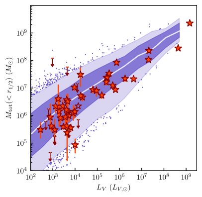
Observed dwarf satellites of the Milky Way exhibit a correlation of the total mass within half-mass radius, , and their luminosity (e.g., see Fig. 4 in Simon, 2019). relations of the observed and model galaxies are compared in Figure 1.
The figure shows that our model reproduces both the normalization and the form of the observed correlation. The median relation shown as a solid line in Figure 1 can be accurately described by the following power law over the entire mass range shown:
| (8) |
This relation reflects relation of and parent halo virial radius and the relation between luminosity and halo mass, as discussed in more detail in the Appendix A. Note that the scatter in the model relation is much larger than the expected scatter of the halo mass within a fixed radius. This is because the scatter in the relation is substantial due to scatter in both and relations.
Agreement between observed and model correlation indicates the model galaxies of a given luminosity form in haloes of correct mass and with values consistent with those of observed galaxies (see also Fig. 12 for an explicit comparison of relations of the galaxies in our model and observed dwarf galaxies Manwadkar & Kravtsov, 2022). We can therefore meaningfully consider both densities and mass assembly histories of the model galaxies to examine the ostensible challenge to CDM.
4.2 Densities of the Milky Way dwarf satellites
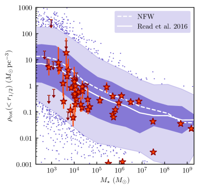
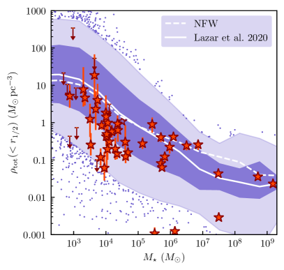
Figure 2 shows , total mass density within , for the model and observed dwarf satellite galaxies located within virial radius of each MW-sized halo in the Caterpillar suite. The two panels show the same measurements for observed satellites (see Section 3.1) by red stars and arrows showing upper limits, while for the model galaxies the mass is computed using parameters of the parent subhalo and model galaxy, but assuming the feedback-modified profiles of Read et al. (2016) in the left panel and of Lazar et al. (2020) in the right panel (see Section 2.1). The median relation in the case when the NFW density profile (not modified by feedback) is assumed instead is shown by the dashed line in each panel.
The effects of feedback expected to modify dark matter density profiles for larger dwarf galaxies are uncertain in the ultra-faint dwarf regime. Several studies indicate that feedback effects should be confined to the galaxies with (Di Cintio et al., 2021; Tollet et al., 2016; Lazar et al., 2020). However, results of Read et al. (2016) indicate that significant modification of the central density distribution occurs in halos of all relevant masses, as long as galaxy is able to form stars for a sufficiently long time.
Regardless of the assumptions about dark matter density profile the model broadly reproduces the overall trend exhibited by observed galaxies, although observed ultra-faint galaxies () tend to have somewhat lower densities than the model ones. We have checked that this is also the case if we only select model dwarf galaxies within the central 70 kpc. The two observed outliers at low density of are Crater II and Antlia II galaxies, which may be undergoing tidal disruption by the Milky Way (Ji et al., 2021; Vivas et al., 2022; Pace et al., 2022, although see Borukhovetskaya et al. 2022)
It is interesting to note that aside from these reported outliers, there is no apparent “diversity problem” – or surprisingly large scatter – in the distribution of for observed dwarf satellites compared to the model results. Such diversity of mass profiles exists for larger dwarf galaxies, where the mass profile is estimated using their observed rotation curves (Oman et al., 2015). This may partly be due to the large scatter in the subhalo profiles compared to their isolated counterparts due to the varying amounts of tidal stripping that they experience.
This overall trend of decreasing density with increasing stellar mass is expected in CDM because 1) galaxies of larger form in halos of larger halo mass , on average, and 2) is roughly a fixed fraction of the virial radius (e.g., Kravtsov, 2013). At a fixed fraction of the virial radius, smaller mass halos are predicted to be denser in the CDM scenario. In fact, in our model for galaxies with , but the proportionality factor drops to for the faintest galaxies. This additional decrease results in a faster increase of towards smaller masses than expected for the CDM haloes at a fixed fraction of the virial radius.

None of the observed galaxies has a surprisingly high density within compared to model expectations. We note that the updated values of velocity dispersion and half-light radius we use for the Horologuium I and Tucana II result in the of and for these galaxies, respectively. The value for Horologium I is lower but comparable to the value of reported by Safarzadeh & Loeb (2021). For Tucana II, on the other hand, they reported an order of magnitude higher density. Nevertheless, even the higher density values reported by these authors are typical for galaxies of according to the model predictions shown in Figure 2.
Kaplinghat et al. (2019) reported a tentative correlation between central densities of the observed classical dwarf galaxies within 150 pc and pericentres of their orbits, estimated using Gaia proper motions. Pace et al. (2022), however, showed that this correlation significantly weakens once pericentres are estimated taking into account gravitational effects of LMC. We examined the distribution of vs pericentre for our model galaxies and did not find any detectable correlations in any of the MW host halos in the Caterpillar suite.
Having established that model approximately reproduces the typical and values estimated for observed MW satellites, we now consider their evolutionary histories.
4.3 Evolution of satellite halo mass and distance from the host halo
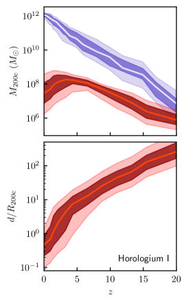
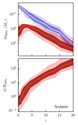
Upper panels of Figure 3 show evolution of halo mass of the main progenitors of the MW-sized hosts and of the subhalos that host galaxies with luminosities similar to those of the Horologium I, Tucana II, and Sculptor. Specifically, we select model galaxies with absolute -band magnitudes within of the value of the corresponding galaxy. We show the evolution of the satellite galaxies with luminosity similar to Horologium I and Tucana II as Safarzadeh & Loeb (2021) argued that these galaxies pose a challenge for CDM. The Fornax galaxy is shown because it is an example of a massive dwarf satellite, for which the progenitor halo mass at high is particularly close to the halo mass of the MW progenitor. Overall, the evolution shown in these three panels is typical of all model satellite galaxies.
The figure shows that the inference that satellites typically have halo mass comparable to that of the MW progenitor at high is correct. This typically occurs at for low-mass systems and at for higher-mass systems. However, as shown in the lower panels of Figure 3, when halo masses of the satellite and MW progenitors were close, these progenitors have been virial radii apart. This prevented their merger during these early epochs. At later times, when progenitors move closer and the satellite progenitor crosses the virial radius of the MW progenitor, the halo mass ratio is and dynamical friction is inefficient.
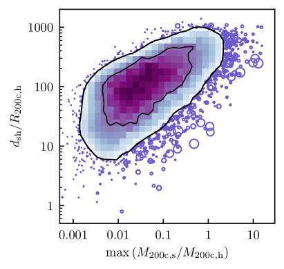
Figure 4 shows the distance between satellite and MW progenitors (in units of the MW progenitor’s ) at the time when the ratio of satellite and host halo progenitor masses was largest, . Remarkably, the figure shows that quite a few surviving satellites had halo masses up to a factor of larger than the MW progenitor at some early epochs. However, this must have occurred well before these objects were accreted onto MW because by definition the main progenitor of the MW must have had a larger halo mass at the time of accretion.
Figure 4 also shows that surviving subhaloes that had masses of the MW progenitor mass were all at more than 10 virial radii apart. Conversely, Figure 4 shows that the lower right corner is devoid of objects. This may be because halos that may have occupied this corner of this parameter space were too close to the Milky Way progenitor and did not survive to .
The progenitor masses of the satellite and MW haloes have similar masses at the earliest epochs because they collapse from small-scale perturbations, which are more likely to have similar amplitude and formation redshifts due to the flattness of the CDM fluctuation amplitude spectrum at small scales. However, their subsequent evolution is determined by the amplitude of the surrounding density perturbation on a larger scale or, equivalently, by the amount of mass in their immediate vicinity available for accretion by these progenitors. The MW progenitor is thus closer to the center of the large-scale density perturbation and has large amounts of mass available for accretion, while the progenitor of the satellite is located at the periphery of the perturbation and accretes at a smaller rate.
As mass difference grows, the MW progenitor starts to dominate its environment and can stun the mass growth of neighboring halos via tidal forces. A similar divergence of mass evolution of comparable mass halos was discussed by Bose & Deason (2022), who found that some halos of mass at evolve into MW-sized halos today, while others either grow much slower or merge with massive neighbors.
5 Summary and conclusions
We use the GRUMPY galaxy formation model based on a suite of zoom-in, high-resolution, dissipationless simulations of the MW-sized haloes from the Caterpillar suite of zoom-in CDM simulations to examine matter density, , within the half-mass radius of stellar distribution and mass evolution of satellite dwarf galaxies around the Milky Way hosts.
We compared matter densities predicted by the model to estimates of such density for 52 observed dwarf satellites of the Milky Way spanning the entire observed luminosity range using an up-to-date compilation of absolute magnitudes, half-light radii, and line-of-sight velocity dispersion measurements (Section 3 and Appendix B). Our main results and conclusions are as follows.
-
(i)
We show that the model reproduces the normalization and shape of the correlation between the total mass within half-light radius, and -band luminosity of observed MW satellites (see Figure 1), which indicates that the model forms galaxies of correct luminosity and size in haloes of a given mass.
-
(ii)
We find that observed dwarf satellites of the Milky Way exhibit a trend of decreasing total matter density within half-light radius, , with increasing stellar mass. This trend is in general agreement with the trend predicted by our model, especially for galaxies with .
-
(iii)
None of the observed satellites are overly dense compared to the results of our CDM-based model and the scatter of their values is comparable to model expectations.
-
(iv)
We show that although at halo masses of many progenitors of satellites surviving to become comparable to or larger than the halo mass of the Milky Way progenitor, at that time the satellite and MW progenitors are separated by the distance of dozens or even hundreds of virial radii. Thus these objects do not merge during these early epochs. At the same time, because MW progenitor halo mass evolves much faster that of the satellite progenitor, by the time the latter accrete onto MW progenitor, they have typically mass ratios of (with the exception of rare major merger accretion events when and MW progenitor accretes an LMC-sized object).
Our results show that neither the densities estimated in observed Milky Way satellites nor their mass assembly histories pose a challenge to the CDM model. In fact, the broad agreement between density trends with the stellar mass of the observed and model galaxies both in their form and scatter can be viewed as yet another success of the model. More detailed further examinations and comparisons will be warranted in the future as estimates of structural parameters and velocity dispersions of observed galaxies improve, especially for the faintest satellite galaxies.
Acknowledgements
We thank Alexander Ji and the Caterpillar collaboration for providing halo tracks of the Caterpillar simulations used in this study and Anirudh Chiti for providing us with his compilation of observational data for the Local Group dwarfs based on the updated list of values from Table 1 of Simon (2019), which we used as a starting point for compiling the table presented in the Appendix. This work was supported by the National Science Foundation grants AST-1714658 and AST-1911111 and NASA ATP grant 80NSSC20K0512. Analyses presented in this paper were greatly aided by the following free software packages: NumPy (Van Der Walt et al., 2011), SciPy (Jones et al., 01 ), Matplotlib (Hunter, 2007), and GitHub. We have also used the Astrophysics Data Service (ADS) and arXiv preprint repository extensively during this project and the writing of the paper.
Data Availability
Halo catalogs from the Caterpillar simulations is available at https://www.caterpillarproject.org/. The GRUMPY model pipeline is available at https://github.com/kibokov/GRUMPY. The data used in the plots within this article are available on request to the corresponding author.
References
- Amorisco & Evans (2011) Amorisco N. C., Evans N. W., 2011, MNRAS, 411, 2118
- Behroozi et al. (2013) Behroozi P. S., Wechsler R. H., Wu H.-Y., Busha M. T., Klypin A. A., Primack J. R., 2013, ApJ, 763, 18
- Behroozi et al. (2022) Behroozi P., Hearin A., Moster B. P., 2022, MNRAS, 509, 2800
- Borukhovetskaya et al. (2022) Borukhovetskaya A., Navarro J. F., Errani R., Fattahi A., 2022, MNRAS, 512, 5247
- Bose & Deason (2022) Bose S., Deason A. J., 2022, arXiv e-prints, p. arXiv:2209.05493
- Boylan-Kolchin et al. (2011) Boylan-Kolchin M., Bullock J. S., Kaplinghat M., 2011, MNRAS, 415, L40
- Bruce et al. (2023) Bruce J., Li T. S., Pace A. B., Heiger M., Song Y.-Y., Simon J. D., 2023, arXiv e-prints, p. arXiv:2302.03708
- Bullock & Boylan-Kolchin (2017) Bullock J. S., Boylan-Kolchin M., 2017, ARA&A, 55, 343
- Buttry et al. (2022) Buttry R., et al., 2022, MNRAS, 514, 1706
- Campbell et al. (2017) Campbell D. J. R., et al., 2017, MNRAS, 469, 2335
- Cantu et al. (2021) Cantu S. A., et al., 2021, ApJ, 916, 81
- Carlin & Sand (2018) Carlin J. L., Sand D. J., 2018, ApJ, 865, 7
- Carlin et al. (2009) Carlin J. L., Grillmair C. J., Muñoz R. R., Nidever D. L., Majewski S. R., 2009, ApJ, 702, L9
- Cerny et al. (2023) Cerny W., et al., 2023, ApJ, 942, 111
- Chiti et al. (2022) Chiti A., Simon J. D., Frebel A., Pace A. B., Ji A. P., Li T. S., 2022, ApJ, 939, 41
- Chiti et al. (2023) Chiti A., et al., 2023, AJ, 165, 55
- Churazov et al. (2010) Churazov E., et al., 2010, MNRAS, 404, 1165
- Conroy & Gunn (2010) Conroy C., Gunn J. E., 2010, ApJ, 712, 833
- Conroy et al. (2009) Conroy C., Gunn J. E., White M., 2009, ApJ, 699, 486
- Correnti et al. (2009) Correnti M., Bellazzini M., Ferraro F. R., 2009, MNRAS, 397, L26
- Di Cintio et al. (2021) Di Cintio A., Mostoghiu R., Knebe A., Navarro J., 2021, arXiv e-prints, p. arXiv:2103.02739
- Di Teodoro et al. (2019) Di Teodoro E. M., et al., 2019, MNRAS, 483, 392
- Errani et al. (2018) Errani R., Peñarrubia J., Walker M. G., 2018, MNRAS, 481, 5073
- Feldmann (2013) Feldmann R., 2013, MNRAS, 433, 1910
- Fritz et al. (2019) Fritz T. K., Carrera R., Battaglia G., Taibi S., 2019, A&A, 623, A129
- Gaia Collaboration et al. (2021) Gaia Collaboration et al., 2021, A&A, 649, A7
- González-Samaniego et al. (2017) González-Samaniego A., Bullock J. S., Boylan-Kolchin M., Fitts A., Elbert O. D., Hopkins P. F., Kereš D., Faucher-Giguère C.-A., 2017, MNRAS, 472, 4786
- Griffen et al. (2016) Griffen B. F., Ji A. P., Dooley G. A., Gómez F. A., Vogelsberger M., O’Shea B. W., Frebel A., 2016, ApJ, 818, 10
- Hunter (2007) Hunter J. D., 2007, Computing In Science & Engineering, 9, 90
- Jenkins et al. (2021) Jenkins S. A., Li T. S., Pace A. B., Ji A. P., Koposov S. E., Mutlu-Pakdil B., 2021, ApJ, 920, 92
- Ji et al. (2021) Ji A. P., et al., 2021, ApJ, 921, 32
- Ji et al. (2023) Ji A. P., et al., 2023, AJ, 165, 100
- Jones et al. (01 ) Jones E., Oliphant T., Peterson P., et al., 2001--, SciPy: Open source scientific tools for Python, http://www.scipy.org/
- Kaplinghat et al. (2019) Kaplinghat M., Valli M., Yu H.-B., 2019, MNRAS, 490, 231
- Kim et al. (2016) Kim D., et al., 2016, ApJ, 833, 16
- Kirby et al. (2013) Kirby E. N., Boylan-Kolchin M., Cohen J. G., Geha M., Bullock J. S., Kaplinghat M., 2013, ApJ, 770, 16
- Kirby et al. (2015) Kirby E. N., Simon J. D., Cohen J. G., 2015, ApJ, 810, 56
- Koposov et al. (2015) Koposov S. E., Belokurov V., Torrealba G., Evans N. W., 2015, ApJ, 805, 130
- Koposov et al. (2018) Koposov S. E., et al., 2018, MNRAS, 479, 5343
- Kravtsov (2013) Kravtsov A. V., 2013, ApJ, 764, L31
- Kravtsov & Manwadkar (2022) Kravtsov A., Manwadkar V., 2022, MNRAS, 514, 2667
- Kravtsov et al. (2018) Kravtsov A. V., Vikhlinin A. A., Meshcheryakov A. V., 2018, Astronomy Letters, 44, 8
- Krumholz & Dekel (2012) Krumholz M. R., Dekel A., 2012, ApJ, 753, 16
- Lazar et al. (2020) Lazar A., et al., 2020, MNRAS, 497, 2393
- Li et al. (2017) Li T. S., et al., 2017, ApJ, 838, 8
- Li et al. (2018) Li T. S., et al., 2018, ApJ, 857, 145
- Lilly et al. (2013) Lilly S. J., Carollo C. M., Pipino A., Renzini A., Peng Y., 2013, ApJ, 772, 119
- Longeard et al. (2018) Longeard N., et al., 2018, MNRAS, 480, 2609
- Longeard et al. (2020) Longeard N., et al., 2020, MNRAS, 491, 356
- Longeard et al. (2021) Longeard N., et al., 2021, MNRAS, 503, 2754
- Manwadkar & Kravtsov (2022) Manwadkar V., Kravtsov A. V., 2022, MNRAS, 516, 3944
- Martínez-Vázquez et al. (2021) Martínez-Vázquez C. E., et al., 2021, AJ, 162, 253
- Mau et al. (2020) Mau S., et al., 2020, ApJ, 890, 136
- Muñoz et al. (2018) Muñoz R. R., Côté P., Santana F. A., Geha M., Simon J. D., Oyarzún G. A., Stetson P. B., Djorgovski S. G., 2018, ApJ, 860, 66
- Mutlu-Pakdil et al. (2018) Mutlu-Pakdil B., et al., 2018, ApJ, 863, 25
- Nadler et al. (2020) Nadler E. O., et al., 2020, ApJ, 893, 48
- Navarro et al. (1997) Navarro J. F., Frenk C. S., White S. D. M., 1997, ApJ, 490, 493
- Oh et al. (2015) Oh S.-H., et al., 2015, AJ, 149, 180
- Oman et al. (2015) Oman K. A., et al., 2015, MNRAS, 452, 3650
- Pace et al. (2022) Pace A. B., Erkal D., Li T. S., 2022, ApJ, 940, 136
- Read & Erkal (2019) Read J. I., Erkal D., 2019, MNRAS, 487, 5799
- Read et al. (2016) Read J. I., Iorio G., Agertz O., Fraternali F., 2016, MNRAS, 462, 3628
- Safarzadeh & Loeb (2021) Safarzadeh M., Loeb A., 2021, arXiv e-prints, p. arXiv:2107.03478
- Sales et al. (2022) Sales L. V., Wetzel A., Fattahi A., 2022, Nature Astronomy, 6, 897
- Silverman et al. (2023) Silverman M., Bullock J. S., Kaplinghat M., Robles V. H., Valli M., 2023, MNRAS, 518, 2418
- Simon (2019) Simon J. D., 2019, ARA&A, 57, 375
- Simon & Geha (2007) Simon J. D., Geha M., 2007, ApJ, 670, 313
- Simon et al. (2011) Simon J. D., et al., 2011, ApJ, 733, 46
- Simon et al. (2020) Simon J. D., et al., 2020, ApJ, 892, 137
- Somerville et al. (2018) Somerville R. S., et al., 2018, MNRAS, 473, 2714
- Spencer et al. (2017) Spencer M. E., Mateo M., Walker M. G., Olszewski E. W., 2017, ApJ, 836, 202
- Suess et al. (2019) Suess K. A., Kriek M., Price S. H., Barro G., 2019, ApJ, 885, L22
- Tollet et al. (2016) Tollet E., et al., 2016, MNRAS, 456, 3542
- Torrealba et al. (2016a) Torrealba G., Koposov S. E., Belokurov V., Irwin M., 2016a, MNRAS, 459, 2370
- Torrealba et al. (2016b) Torrealba G., et al., 2016b, MNRAS, 463, 712
- Torrealba et al. (2018) Torrealba G., et al., 2018, MNRAS, 475, 5085
- Van Der Walt et al. (2011) Van Der Walt S., Colbert S. C., Varoquaux G., 2011, ArXiv:1102.1523, p. 1
- Vivas et al. (2022) Vivas A. K., Martínez-Vázquez C. E., Walker A. R., Belokurov V., Li T. S., Erkal D., 2022, ApJ, 926, 78
- Walker et al. (2009) Walker M. G., Mateo M., Olszewski E. W., Peñarrubia J., Evans N. W., Gilmore G., 2009, ApJ, 704, 1274
- Willman et al. (2011) Willman B., Geha M., Strader J., Strigari L. E., Simon J. D., Kirby E., Ho N., Warres A., 2011, AJ, 142, 128
- Wolf et al. (2010) Wolf J., Martinez G. D., Bullock J. S., Kaplinghat M., Geha M., Muñoz R. R., Simon J. D., Avedo F. F., 2010, MNRAS, 406, 1220
Appendix A The origin of the relation
The power law relation between the total mass within the half-mass radius and -band galaxy luminosity discussed in Section 4.1 (see eq. 8 and Figure 1) reflects the relation of and parent halo virial radius and the relation between luminosity and halo mass.
For example, suppose we assume 1) the approximately linear (Kravtsov, 2013), 2) the approximately power law relation, , where (e.g., Kravtsov et al., 2018; Read & Erkal, 2019; Nadler et al., 2020), 3) that dark matter dominates within , and thus we can use NFW mass profile. Then can be approximated by the equation 3, which shows that with the factor of proportionality , where is halo concentration. This factor is only weakly dependent on , such that the overall relation can be accurately approximated by .
Thus, using the relation we get . For the power law index is , which is shallower than the relation we find for our model and observed galaxies. The main reason for this is that the relation in the model galaxies is steeper than linear at the smallest masses and exhibits large scatter and this steepens the relation to , which, in turn, results in relation that describes the correlation shown in Figure 1.
Appendix B Observational data
Table LABEL:tab:sample shows the values of the -band absolute magnitudes, , half-light radii, , and line-of-sight velocity dispersions of the Milky Way satellites used in this study. The basis of the sample is the Supplemental Table 1 in Simon (2019) review. This compilation was augmented with new measurements for existing dwarfs (e.g., new measurements of velocity dispersion for the Aquarius II, Reticulum, Tucana II, etc. Bruce et al., 2023; Ji et al., 2023; Chiti et al., 2023) and for several newly discovered ultra-faint dwarfs, such as Pegasus IV (Cerny et al., 2023) to the extent that we could identify such measurements. We used uniform measurements of structural properties and and half-light radii from the Megacam-based study of Muñoz et al. (2018) for galaxies for which these are available. Their half-light estimate for the Plummer model is used for half-light radii, because the Plummer model provides one of the best matches to the projected stellar surface density profiles of these galaxies.
The last column in Table LABEL:tab:sample provides references for the estimates of galaxy properties. The first reference(s) refer to and estimates, and the last reference to the velocity dispersion estimate, unless both were made in a single paper in which case a single reference is given. For some galaxies only upper limit on the velocity dispersion was obtained so far. We plot these as upper limits on mass and density in our analyses. For Centaurus I velocity dispersion km/s is reported by Martínez-Vázquez et al. (2021) without uncertainties and this galaxy is shown by open star without error bar in our plots.
Unlike other galaxies in the sample LMC and SMC are not dwarf spheroidals but of the irregular type. Velocity dispersions listed in the table for these galaxies are not the actual velocity dispersions, but rather values that would give the same as obtained from the estimate , where is measured rotation velocity at . For the latter we use values listed and the table and published rotation curves for the LMC (Gaia Collaboration et al., 2021, see their Fig. 14) and SMC (Di Teodoro et al., 2019) to estimate km/s and km/s.
We note that it is still debated whether some of the objects included in our sample are star clusters or galaxies (e.g., Sagittarius II, Phoenix II). We choose to do so because there is still a possibility that these may be galaxies and because velocity dispersions and half-light radii of such systems are consistent with them being dwarf galaxies. Likewise, we include galaxies which may be heavily influenced by tidal stripping, such as Antlia II, Crater II, Tucana III because we want to retain the full range of values in the observed satellites.
| Galaxy name | References | |||
|---|---|---|---|---|
| (pc) | km/s | |||
| Antlia II | Ji et al. (2021) | |||
| Aquarius II | Torrealba et al. (2016b); Bruce et al. (2023) | |||
| Boötes I | Jenkins et al. (2021) | |||
| Boötes II | Muñoz et al. (2018); Bruce et al. (2023) | |||
| Boötes III | Correnti et al. (2009); Carlin et al. (2009); Carlin & Sand (2018) | |||
| Canes Venatici I | Muñoz et al. (2018); Simon & Geha (2007) | |||
| Canes Venatici II | Muñoz et al. (2018); Simon & Geha (2007) | |||
| Carina | Muñoz et al. (2018); Walker et al. (2009) | |||
| Carina II | Torrealba et al. (2018); Li et al. (2018) | |||
| Carina III | Torrealba et al. (2018); Li et al. (2018) | |||
| Centaurus I | Mau et al. (2020); Martínez-Vázquez et al. (2021) | |||
| Columba I | Muñoz et al. (2018); Fritz et al. (2019) | |||
| Coma Berenices | Muñoz et al. (2018); Simon & Geha (2007) | |||
| Crater II | Torrealba et al. (2016a), Ji et al. (2021) | |||
| Draco | Muñoz et al. (2018); Walker et al. (2009) | |||
| Draco II | Longeard et al. (2018) | |||
| Eridanus II | Muñoz et al. (2018); Li et al. (2017) | |||
| Fornax | Muñoz et al. (2018); Walker et al. (2009) | |||
| Grus I | Cantu et al. (2021); Chiti et al. (2022) | |||
| Grus II | Simon et al. (2020) | |||
| Hercules | Muñoz et al. (2018); Simon & Geha (2007) | |||
| Horologium I | Muñoz et al. (2018); Koposov et al. (2015) | |||
| Horologium II | Muñoz et al. (2018); Fritz et al. (2019) | |||
| Hydra II | Muñoz et al. (2018); Kirby et al. (2015) | |||
| Hydrus I | Koposov et al. (2018) | |||
| Leo I | Muñoz et al. (2018); Walker et al. (2009) | |||
| Leo II | Muñoz et al. (2018); Spencer et al. (2017) | |||
| Leo IV | Jenkins et al. (2021) | |||
| Leo V | Jenkins et al. (2021) | |||
| Leo T | Muñoz et al. (2018); Simon & Geha (2007) | |||
| LMC | Muñoz et al. (2018), see text | |||
| Pegasus III | Kim et al. (2016) | |||
| Pegasus IV | Cerny et al. (2023) | |||
| Phoenix II | Muñoz et al. (2018); Fritz et al. (2019) | |||
| Pisces II | Muñoz et al. (2018); Kirby et al. (2015) | |||
| Reticulum II | Muñoz et al. (2018); Ji et al. (2023) | |||
| Reticulum III | Muñoz et al. (2018); Fritz et al. (2019) | |||
| Sagittarius | Simon (2019) | |||
| Sagittarius II | Longeard et al. (2020, 2021) | |||
| Sculptor | Muñoz et al. (2018); Walker et al. (2009) | |||
| Segue 1 | Muñoz et al. (2018); Simon et al. (2011) | |||
| Segue 2 | Muñoz et al. (2018); Kirby et al. (2013) | |||
| Sextans | Muñoz et al. (2018); Walker et al. (2009) | |||
| SMC | Muñoz et al. (2018), see text | |||
| Triangulum II | Muñoz et al. (2018); Buttry et al. (2022) | |||
| Tucana II | Koposov et al. (2015); Chiti et al. (2023) | |||
| Tucana III | Mutlu-Pakdil et al. (2018); Simon (2019) | |||
| Tucana IV | Simon et al. (2020) | |||
| Tucana V | Simon et al. (2020) | |||
| Ursa Major I | Muñoz et al. (2018); Simon (2019) | |||
| Ursa Major II | Muñoz et al. (2018); Simon (2019) | |||
| Ursa Minor | Muñoz et al. (2018); Walker et al. (2009) | |||
| Willman 1 | Muñoz et al. (2018); Willman et al. (2011) |