The Power of Populations in Decentralized Bandits

Abstract

We study a cooperative multi-agent bandit setting in the distributed GOSSIP model: in every round, each of $n$ agents chooses an action from a common set, observes the action’s corresponding reward, and subsequently exchanges information with a single randomly chosen neighbor, which informs its policy in the next round. We introduce and analyze several families of fully-decentralized local algorithms in this setting under the constraint that each agent has only constant memory. We highlight a connection between the global evolution of such decentralized algorithms and a new class of “zero-sum” multiplicative weights update methods, and we develop a general framework for analyzing the population-level regret of these natural protocols. Using this framework, we derive sublinear regret bounds for both stationary and adversarial reward settings. Moreover, we show that these simple local algorithms can approximately optimize convex functions over the simplex, assuming that the reward distributions are generated from a stochastic gradient oracle.

1 Introduction

The multi-armed bandit problem, where a single learning agent chooses actions over a sequence of rounds in order to maximize its total reward, is among the most well-studied in online learning. Distributed, multi-agent variants of this problem have also been widely studied under various constraints; one particular such line of work is the cooperative multi-agent bandit setting, where agents are connected over a communication graph and play against a common bandit instance, choosing actions in parallel over $T$ rounds. Each agent locally runs a bandit algorithm that may involve communication with neighbors, and the information exchanged can be used to determine an agent’s future actions. This cooperative setting has been studied for both stochastic (Szorenyi et al., 2013; Landgren et al., 2016; Kolla et al., 2018; Martínez-Rubio et al., 2019) and non-stochastic bandits (Awerbuch & Kleinberg, 2008; Cesa-Bianchi et al., 2016; Bar-On & Mansour, 2019), where communication between agents has been shown to improve an agent’s regret on average, compared to each agent locally running a centralized bandit algorithm without any communication.

However, most prior works in this setting require that every agent communicate with all its neighbors in each round (as pointed out by Cesa-Bianchi et al. (2016), this resembles the LOCAL model of distributed computation (Linial, 1992)). When the underlying graph is dense, this volume of communication may be prohibitively large, which is a known bottleneck in many practical distributed machine learning settings (Alistarh et al., 2017; Koloskova et al., 2019a; b).

In contrast, much less is known about cooperative multi-agent bandits in more lightweight decentralized models of distributed communication, such as the GOSSIP model (Boyd et al., 2006; Shah et al., 2009). In this model, at every round, each agent is randomly connected to one of its neighbors, and thus the total number of information exchanges per-round scales only linearly in the size of the population, even for dense communication graphs. Algorithms for general distributed tasks have been studied extensively in the GOSSIP model (Aldous & Lanoue, 2012; Aldous, 2013; Becchetti et al., 2020) and specifically in modern machine learning settings (Lian et al., 2017; Assran et al., 2019; Even et al., 2021). Yet, much less is known about the power of this model in the cooperative multi-agent bandit setting, which is the focus of this paper. For concreteness, we begin by introducing our setting precisely.

1.1 Problem Setting

Consider a population of $n$ agents distributed over a communication graph $G$. The $n$ agents interact with a common $m$-armed bandit instance over a sequence of $T$ rounds, each of which is structured as follows:

1. Action Choices: At the start of each round $t$, each agent $u\in[n]$ chooses an action $j\in[m]$.

2. Reward Generation and Observation: In every round $t$, each action $j\in[m]$ generates a reward $g^{t}_{j}\sim\nu^{t}_{j}$, where $\mathbb{E}[g^{t}_{j}]=\mu^{t}_{j}$. Each node choosing action $j$ subsequently observes the reward $g^{t}_{j}$.

3. Communication: Then, each agent simultaneously samples a single neighbor to receive information from, uniformly at random. Each agent may use this interaction to determine its action in the next round.

At each round $t$, we denote by $\mathbf{g}^{t}:=(g^{t}_{1},\dots,g^{t}_{m})$ and $\boldsymbol{\mu}^{t}:=(\mu^{t}_{1},\dots,\mu^{t}_{m})$ the $t$’th reward vector and mean reward vector respectively, and we distinguish between a stationary reward setting, where $\boldsymbol{\mu}^{t}=\boldsymbol{\mu}$ is fixed, and an adversarial reward setting, where these means may vary:

• Stationary reward setting: For each action $j\in[m]$ and round $t\in[T]$, the distribution $\nu^{t}_{j}$ has mean $\mu_{j}\in[0,1]$ and is supported on $[0,\sigma]$ for some $\sigma\geq 1$. Without loss of generality, assume $\mu_{1}>\mu_{2}\geq\dots\geq\mu_{m}$.

• Adversarial reward setting: For each action $j\in[m]$ and round $t\in[T]$, the distribution $\nu^{t}_{j}$ has mean $\mu^{t}_{j}\in[-1,1]$ and support $[-\sigma,\sigma]$ for some fixed $\sigma\geq 1$.

Given some (randomized) local algorithm run by each agent in the population, we measure its performance using the following notion of regret: first, let $\mathbf{p}^{t}:=(p^{t}_{1},\dots,p^{t}_{m})\in\Delta_{m}$ denote the distribution specifying the fraction of the agents choosing each action $j$ at round $t$, and at round $t=0$, assume each agent is deterministically given some initial action choice $j$ such that $\mathbf{p}^{0}=(1/m,\dots,1/m)$. Then for the sequence of distributions $\{\mathbf{p}^{t}\}$ induced by the algorithm, we define its expected population-level regret as

$$R(T)\;:=\;\max_{j\in[m]}\sum_{t\in[T]}\mu^{t}_{j}\;-\;\sum_{t\in[T]}\mathbb{E}[\langle\mathbf{p}^{t},\mathbf{g}^{t}\rangle]\;.$$

We say the regret $R(T)$ is sublinear when the average regret $R(T)/T$ goes to 0 with both $T$ (the number of rounds) and $n$ (the number of agents). Note the following observations:

• First, other than the GOSSIP-style communication, the problem setting is identical to that of Cesa-Bianchi et al. (2016) and Bar-On & Mansour (2019). In particular, each action at round $t$ generates a single reward that is observed by all agents choosing that action.

• The population-level regret $R(T)$ (henceforth referred to as “regret”) can be viewed as the cumulative expected regret of the average agent in the population (i.e., under the distributions $\{\mathbf{p}^{t}\}$). This regret notion is thus equivalent to those used in other cooperative bandits works, e.g., (Landgren et al., 2016; Martínez-Rubio et al., 2019; Bar-On & Mansour, 2019), when averaged over agents.

Related work with GOSSIP communication

Closely-related settings were recently studied by Celis et al. (2017), Su et al. (2019), and Sankararaman et al. (2019). However, each of these works considered only stationary rewards with fixed-mean Bernoulli distributions. Moreover, the algorithms developed assume that either agents have large amounts of local memory (Celis et al., 2017; Su et al., 2019; Sankararaman et al., 2019), that agents can refrain from choosing an action in some rounds (Celis et al., 2017; Su et al., 2019), or that agent communication is implicitly performed through a central server (Celis et al., 2017).

Memory and Decentralization Constraints

In contrast to these previous works, our focus is on algorithms that are fully-decentralized, light-weight in terms of local memory, and robust to adversarial rewards. Specifically, we assume:

1. Each agent has only constant local memory (w.r.t. $m$, $n$, and $T$). For instance, this means that agents are unable to maintain a probability distribution or store a history of rewards over the full set of $m$ actions.

2. Agents are identical and anonymous (i.e., have no identifiers), and each agent runs the same local algorithm at each round without any central coordination.

The first constraint is motivated by systems comprised of low-memory devices such as sensor networks, which are commonly analyzed in the GOSSIP model (Boyd et al., 2006; Shah et al., 2009), and also settings like recommender systems where the size of the action set is extremely large, and agents cannot maintain information for each possible action. In particular, this precludes agents from each locally running a classic bandit algorithm like UCB or EXP3. Also, under these memory constraints, when initialized from $\mathbf{p}^{0}=\mathbf{1}/m$ and with no communication, the regret $R(T)$ is necessarily at least $T/2$, since the memory constraints mean agents can each only choose from a constant set of fixed actions every round. Thus, new algorithmic ideas are required to leverage the GOSSIP-style communication.

The second constraint limits our study to algorithms that are fully decentralized and cannot rely on building global structures, partitioning agents into separate roles, or assume a central server capable of coordinating the behavior of agents. This type of decentralization is increasingly studied in other learning and optimization settings (Lian et al., 2017; Koloskova et al., 2019b) and is motivated by settings where agents may be subject to privacy or communication constraints. Moreover, designing and analyzing decentralized algorithms in the present setting is a first step in studying systems prone to communication errors, time-varying topologies, and when interchangeable agents may enter and leave the population over time (Martínez-Rubio et al., 2019).

1.2 Our Contributions

We introduce and analyze families of local algorithms for this setting that satisfy properties (i) and (ii) above, for which we prove sublinear regret bounds in both the stationary and adversarial reward settings assuming a complete communication graph. Specifically, we introduce algorithms in which each agent chooses its action in round $t+1$ based only on its action and reward from round $t$, and that of the single random neighbor it communicated with. Our analysis provides regret bounds that highlight the robustness of these simple algorithms to both stationary and adversarial reward settings, and moreover, they consistently highlight the effect that larger populations tend to reduce regret:

• For the stationary reward setting (Theorem 2.8) and sufficiently large $n$, our algorithms obtain average regret

  $$\frac{R(T)}{T}\;\leq\;O\bigg{(}\frac{\log m}{T}\bigg{)}+\widetilde{O}\bigg{(}\frac{\sigma m}{\sqrt{n}}\bigg{)}\;.$$

• For the adversarial reward setting (Theorem 2.9), our algorithms obtain average regret

  $$\frac{R(T)}{T}\;\leq\;O\bigg{(}\sqrt{\frac{\log m}{T}}\bigg{)}+\widetilde{O}\bigg{(}\frac{\sigma m}{n^{\epsilon}}\bigg{)}\;,$$

  for $n$ sufficiently large, but in particular for $T$ at most $(\frac{1}{2}-\epsilon)\log_{5}n$ rounds, for any $\epsilon\in(0,\frac{1}{2})$.

Discussion

In both reward settings, our average regret bounds vanish with both $T$ and $n$. By virtue of our analysis framework, these bounds are decomposed into two terms: the first is an approximation error, where we bound the regret of the sequence $\{\mathbf{p}^{t}\}$ induced by our algorithms by the regret of a smoother process. The second is an estimation error, which is incurred by this approximation.

In our bounds, the approximation error terms scale like $O((\log m)/T)$ and $O(\sqrt{(\log m)/T})$ for the stationary and adversarial reward settings, respectively. As our regret notion can be viewed as the average regret per agent in the population, notice that these approximation terms improve over the optimal single-agent time-averaged regret bounds of $O((\log(mT)/T)$ and $O(\sqrt{(m\log m)/T})$ for the stationary (assuming constant suboptimality gap) and adversarial reward settings, respectively (Bubeck et al., 2012; Lattimore & Szepesvári, 2020).

This improvement is a direct byproduct of the random, pairwise agent communication: although the problem setting resembles a multi-armed bandit instance from the perspective of a single agent, the full reward feedback over all actions is distributed over the population in every round. While similar effects have been observed before in distributed settings with LOCAL communication, where each agent can communicate in every round with all neighbors (Cesa-Bianchi et al., 2016; Bar-On & Mansour, 2019), our results are the first to show that these improved rates can be obtained in a fully decentralized manner with GOSSIP communication. In this perspective, the approximation error terms of our bounds resemble the optimal regret for the prediction with expert advice setting (full information feedback) for both the stationary reward setting (matching the rate for exp-concave loss functions) and the adversarial reward setting (Cesa-Bianchi & Lugosi, 2006; Arora et al., 2012).

On the other hand, the second terms of our bounds, corresponding to an estimation error, scale like $\widetilde{O}(\frac{m}{\sqrt{n}})$ and $\widetilde{O}(\frac{m}{n^{0.25}})$ for the stationary and adversarial reward settings (when $\epsilon=\nicefrac{{1}}{{4}}$), respectively. These terms can be viewed as a cost of anonymity and decentralization in the extremely simple model we consider. In both settings, these terms vanish as the number of agents $n$ grows, and our algorithms for the stationary reward setting enjoy a faster rate of decay compared to the more challenging, adversarial reward setting. Moreover, we show in this adversarial setting and under the algorithmic constraints we consider that regret can grow linearly with $T$ if the number of rounds is larger than logarithmic in the number of agents $n$. For this reason, our bound for the adversarial setting constaints $T=O(\log n)$.

Overall, our results highlight the power of large populations in this multi-agent learning setting: despite the local memory and decentralization constraints we consider, our algorithms leverage the random pairwise agent communications of the GOSSIP-model to obtain sublinear regret bounds that, for both the stationary and adversarial reward settings, diminish with increasing population sizes.

Convex Optimization Application

Additionally we use our framework to obtain expected error rates for approximately optimizing a convex function $f:\Delta_{m}\to\mathbb{R}$ under the assumption that the reward sequence $\{\mathbf{g}^{t}\}$ is generated by a stochastic gradient oracle. Here, we give an error rate at the average iterate $\widetilde{\mathbf{p}}:=\frac{1}{T}\sum_{t\in[T]}\mathbf{p}^{t}$ of the distributions $\{\mathbf{p}^{t}\}$ induced by our algorithms, and this rate matches our regret bound from the adversarial reward setting up to constant factors. This result is presented in Theorem 2.10.

1.3 Summary of Techniques

We introduce families of algorithms that are inspired in part by memory-constrained opinion dynamics studied in the context of other distributed computing tasks (Becchetti et al., 2014a; Ghaffari & Lengler, 2018; Becchetti et al., 2020; Amir et al., 2023), and we bound the regret of these algorithms by carefully analyzing the evolution of the agent action choice distributions $\{\mathbf{p}^{t}\}$ they induce. Surprisingly, we show for each family that the coordinates $p^{t}_{j}$ evolve (in conditional expectation) by multiplicative factors of the form $(1+F_{j}(\mathbf{p}^{t},\mathbf{g}^{t}))$, where each $F_{j}$ is a function depending on $\mathbf{p}^{t}$ and $\mathbf{g}^{t}$ that collectively satisfy the key “zero-sum” property of $\sum_{j\in[m]}p^{t}_{j}\cdot F_{j}(\mathbf{p}^{t},\mathbf{g}^{t})=0$.

We more generally relate processes of this form to a class of (centralized) zero-sum multiplicative weights update (MWU) algorithms, and we derive bounds on their regret that may be of independent interest. This connection is then leveraged to establish a general analysis framework for bounding the regret of the original process $\{\mathbf{p}^{t}\}$. In this sense, our technique adds to a growing body of work that analyzes other distributed or gossip dynamics by relating their evolution to centralized optimization algorithms (Mallmann-Trenn et al., 2018; Even et al., 2021).

We now proceed to give a technical overview of our algorithms, analysis framework, and regret bounds, before concluding with some discussion and open questions. In Appendix A, we also provide several sets of simulations that validate our results experimentally, and we defer a more detailed discussion of other related works to Appendix B.

2 Technical Overview

Notation and Other Preliminaries

Throughout, we deal with multiple sequences of vectors indexed over rounds $t\in[T]$, for which we use the short hand notation $\{\mathbf{p}^{t}\}:=\mathbf{p}^{0},\mathbf{p}^{1},\dots,\mathbf{p}^{t}$. We often compute expectation (resp., probabilities) conditioned on two sequences $\{\mathbf{p}^{t}\}$ and $\{\mathbf{g}^{t}\}$ (or $\{\mathbf{q}^{t}\}$ and $\{\mathbf{g}^{t}\}$) simultaneously, and we denote this double conditioning by $\mathbb{E}_{t}[\cdot]$. When conditioning on just a single vector $\mathbf{p}^{t}$, we write $\mathbb{E}_{\mathbf{p}^{t}}[\cdot]$. Given $\mathbf{p}=(p_{1},\dots,p_{m})$, we write $\mathbb{E}[\mathbf{p}]$ to denote the vector $(\mathbb{E}[p_{1}],\dots,\mathbb{E}[p_{m}])$. Throughout, we use the fact that for a non-negative random variable $x$, if $x\leq\alpha$ w.p. at least $1-\gamma$, then $\mathbb{E}[x]\leq\alpha+\gamma$. We assume all logarithms are natural unless otherwise specified, and we use $\mathbf{1}$ to denote the vector of all ones.

2.1 Families of Local Algorithms

We begin by introducing two simple families of local algorithms for the problem setting: adoption algorithms, and comparison algorithms. These families are defined from the perspective of any agent $u$ at round $t$ as follows:

Adoption Algorithms: given a non-decreasing adoption function $f:\mathbb{R}\to[0,1]$, for each $u\in[n]$: (i) At round $t$, assume: agent $u$ chose action $j$; $u$ sampled agent $v$; and $v$ chose action $k\in[m]$. (ii) At round $t+1$: agent $u$ chooses action $k$ with probability $f(g^{t}_{k})$ and action $j$ otherwise.

Comparison Algorithms: given a non-decreasing score function $h:\mathbb{R}\to\mathbb{R}_{\geq 0}$, for each $u\in[n]$: (i) At round $t$, assume: agent $u$ chose action $j$; $u$ sampled agent $v$; and $v$ chose action $k\in[m]$. (ii) At round $t+1$: define $\rho_{j}\propto h\big{(}g^{t}_{j}\big{)}$ and $\rho_{k}\propto h\big{(}g^{t}_{k}\big{)}$.
Then agent $u$ chooses action $j$ with probability $\rho_{j}$ and action $k$ with probability $\rho_{k}$.

Remarks and Examples

In both families of algorithms, notice that each agent’s choice of action at round $t+1$ is either the action it chose from round $t$, or that of its randomly sampled neighbor under the GOSSIP communication model. Thus in both families, each agent builds a local probability distribution over these two action choices, and it draws its action for the next round according to this distribution.

In every adoption algorithm, each agent’s local distribution for round $t+1$ depends only on the reward $g^{t}_{k}$ obtained by its randomly sampled neighbor in round $t$. The probability of choosing the neighbor’s previous action in the next round is exactly $f(g^{t}_{k})$ (while the probability of an agent repeating its own choice is $1-f(g^{t}_{k})$), where $f$ is the non-decreasing adoption function. This family can be viewed as generalization of the sample and adopt dynamics of Celis et al. (2017). As examples, we consider the following instantiated versions under different choices of $f$:

• $\beta$-$\mathsf{exp}\text{-}\mathsf{adopt}$ is the adoption algorithm with $f_{\beta}(g):=\beta^{g}\cdot(1-\beta)^{1-g}$ for some $\beta\in(0.5,1)$, and assuming binary rewards (i.e., all $\mathbf{g}^{t}\in\{0,1\}^{m}$).

• $\beta$-$\mathsf{disc}\text{-}\mathsf{adopt}$ is the adoption algorithm with $f_{\beta}(g):=\beta\cdot g$ for some $\beta\in(0,1/\sigma]$, and assuming all $\mathbf{g}^{t}\in[0,\sigma]^{m}$.

• $\beta$-$\mathsf{sigmoid}\text{-}\mathsf{adopt}$ is the adoption algorithm with the sigmoid function $f_{\beta}(g):=\frac{1}{1+\exp(-\beta\cdot g)}$ for $\beta\in[0,1]$, and for general rewards $\mathbf{g}^{t}\in[-\sigma,\sigma]^{m}$.

In contrast, in comparison algorithms, each agent’s local distribution for round $t+1$ is now a function of both the reward $g^{t}_{k}$ obtained by its randomly sampled neigbor in round $t$, and also its own reward $g^{t}_{j}$ from round $t$ (in particular, the distribution over actions $j$ and $k$ is simply proportional to the scores of these rewards under the function $h$). At a high-level, this strategy is reminiscent of the power-of-two choices principle (Mitzenmacher, 2001), and also of pairwise comparison strategies from evolutionary game theory (Allen & Nowak, 2014; Schmid et al., 2019). As an example, we consider the following instantiation:

• $\beta$-$\mathsf{softmax}\text{-}\mathsf{compare}$ is the comparison algorithm using the score function $h_{\beta}(g):=\exp(\beta\cdot g)$ for some $\beta\in[0,1]$, and for general rewards $\mathbf{g}^{t}\in[-\sigma,\sigma]^{m}$.

Evolution in Conditional Expectation

Consider the sequence of distributions $\{\mathbf{p}^{t}\}$ induced by running any adoption or comparison algorithm with reward sequence $\{\mathbf{g}^{t}\}$. A natural first step in bounding the population-level regret of $\{\mathbf{p}^{t}\}$ is to analyze its coordinate-wise evolution. Interestingly, for both families, we show in conditional expectation that each $p^{t}_{j}$ evolves multiplicatively by a factor roughly proportional to some relative difference between (a function of) $g^{t}_{j}$ and a weighted average over all coordinates of $\mathbf{g}^{t}$. For example, for adoption algorithms, we obtain the following proposition (proved in Appendix C):

Proposition 2.1.

Let $\{\mathbf{p}^{t}\}$ be the sequence induced when every agent runs the adoption algorithm with function $f$ and reward sequence $\{\mathbf{g}^{t}\}$. Then letting $f(\mathbf{g}^{t})$ denote the coordinate-wise application of $f$ on $\mathbf{g}^{t}$, it holds that $\mathbb{E}_{t}[p^{t+1}_{j}]=p^{t}_{j}\big{(}1+f(g^{t}_{j})-\langle\mathbf{p}^{t},f(\mathbf{g}^{t})\rangle\big{)}$ for every $t$ and $j$.

For comparison algorithms, we obtain a similar multiplicative update form. For this, we use quantities $\rho_{j}$ and $\rho_{k}$ as given in the definition of the algorithm. Then we have the following proposition (also proved in Appendix C):

Proposition 2.2.

Let $\{\mathbf{p}^{t}\}$ be the sequence induced when every agent runs the comparison algorithm with score function $h$ and reward seqeunce $\{\mathbf{g}^{t}\}$. Furthermore, for any $\mathbf{g}\in\mathbb{R}^{m}$ and $j\in[m]$, let $H(\mathbf{g},j)\in[-1,1]^{m}$ be the $m$-dimensional vector whose $k$’th coordinate is given by $\rho_{j}-\rho_{k}$. Then $\mathbb{E}_{t}[p^{t+1}_{j}]=p^{t}_{j}\cdot\big{(}1+\langle\mathbf{p}^{t},H(\mathbf{g}^{t},j)\rangle\big{)}$ for every $t$ and $j$.

To summarize, for adoption algorithms with function $f$, at round $t$, each coordinate $j$ grows according to the strength of $f(g^{t}_{j})$ relative to the weighted average over all $f(g^{t}_{k})$. Similarly, in comparison algorithms with score function $h$, the $j$’th coordinate grows proportionally to the weighted average of differences $h(g^{t}_{j})-h(g^{t}_{k})$ over all other $k$. Letting $\widehat{\mathbf{p}}_{t+1}:=\mathbb{E}_{t}[\mathbf{p}^{t+1}]$, notice that Propositions 2.1 and 2.2 both describe multiplicative updates that can be captured in the following, more general form:

$$\widehat{p}^{t+1}_{j}:=\mathbb{E}_{t}[p^{t+1}_{j}]\;=\;p^{t}_{j}\cdot\big{(}1+F_{j}(\mathbf{p}^{t},\mathbf{g}^{t})\big{)}\;,$$ (1)

where the set of $m$ functions $\{F_{j}\}^{m}_{j=1}$ satisfies the zero-sum condition $\sum_{j\in[m]}p_{j}\cdot F_{j}(\mathbf{p},\mathbf{g})=0$ for all $\mathbf{p}\in\Delta_{m}$ and $\mathbf{g}\in\mathbb{R}^{m}$. For adoption algorithms with function $f$, Proposition 2.1 shows that each $F_{j}(\mathbf{p},\mathbf{g})=f(g_{j})-\langle\mathbf{p},f(\mathbf{g})\rangle$. For comparison algorithms with score function $h$, Proposition 2.2 shows $F_{j}(\mathbf{p},\mathbf{g})=\langle\mathbf{p},H(\mathbf{g},j)\rangle$.

Note that while the coordinates of the distribution $\mathbb{E}_{t}[\mathbf{p}^{t+1}]$ are updated multiplicatively as in (1), the sequence $\{\mathbb{E}_{t}[\mathbf{p}^{t+1}]\}$ is not neceessarily smooth: these updates are applied w.r.t. the realized distribution $\mathbf{p}^{t}$, and not $\mathbb{E}_{t-1}[\mathbf{p}^{t}]$. However, to bound the regret of $\{\mathbf{p}^{t}\}$, we leverage properties of the process $\{\mathbf{q}^{t}\}$ whose coordinates do evolve by composing this update in each round using the same family $\{F_{j}\}$. We define these zero-sum MWU processes as follows:

2.2 Zero-Sum MWU Processes

Consider sequences of distributions $\{\mathbf{q}^{t}\}$ that evolve according to the following definition:

Definition 2.3 (Zero-Sum MWU).

Let $\mathcal{F}=\{F_{j}\}$ be a family of $m$ potential functions $F_{j}:\Delta_{m}\times\mathbb{R}^{m}\to[-1,1]$ satisfying the zero-sum condition $${\textstyle\sum}_{j\in[m]}\;q_{j}\cdot F_{j}(\mathbf{q},\mathbf{g})=0$$ (2) for all $\mathbf{q}\in\Delta_{m}$ and $\mathbf{g}\in\mathbb{R}^{m}$. Then initialized from $\mathbf{q}^{0}\in\Delta_{m}$ and given $T$, we say $\{\mathbf{q}^{t}\}$ is a zero-sum MWU process with reward sequence $\{\mathbf{g}^{t}\}$ if for all $t\in[T]$ and $j\in[m]$: $$q^{t+1}_{j}\;=\;q^{t}_{j}\cdot\big{(}1+F_{j}\big{(}\mathbf{q}^{t},\mathbf{g}^{t}\big{)}\big{)}\;.$$ (3)

Compared to the standard (polynomial) versions of multiplicative weights update methods (Arora et al., 2012), the zero-sum condition (2) always ensures the set of updated weights in (3) remains a distribution, without an additional renormalization step (i.e., the simplex $\Delta_{m}$ is invariant to $\{\mathbf{q}^{t}\}$). We remark that these types of zero-sum multiplicative updates are commonly known as replicator dynamics in the continuous time setting, where one considers systems of the form $(dq^{t}_{j}/dt)=(u(g^{t}_{j})-\langle\mathbf{q}^{t},u(\mathbf{g}^{t}_{j})\rangle)$ for some utility function $u$, usually in the context of evolutionary dynamics and game theory (Schuster & Sigmund, 1983; Hofbauer et al., 1998; Cabrales, 2000; Panageas & Piliouras, 2016).

On the other hand, discrete-time MWU processes with update factors satisfying the zero-sum condition in (2) have not been as well-studied, particularly in the context of the prediction with expert advice or multi-armed bandit settings, where one wishes to bound regret with respect to $\{\mathbf{g}^{t}\}$ directly (and not with respect to some function of $\mathbf{g}^{t}$). In our analysis framework below, we develop such regret bounds for these processes with respect to $\{\mathbf{g}^{t}\}$, where the bounds depend on some quality measure of the family $\mathcal{F}$ in distinguishing higher-mean and lower-mean rewards.

2.3 Analysis Framework for Bounding $R(T)$

We now introduce a general analysis framework for bounding the regret of the sequence $\{\mathbf{p}^{t}\}$ induced by any dynamics with conditionally expected updates as in expression (1). As previously alluded to, our strategy relies on introducing a true zero-sum MWU process $\{\mathbf{q}^{t}\}$ that starts at the same initial distribution as $\{\mathbf{p}^{t}\}$, runs on the same reward sequence, and uses the same family $\mathcal{F}$ as follows:

Definition 2.4 (Coupled Trajectories).

Let $\mathcal{F}=\{F_{j}\}$ be a family of zero-sum functions as in Definition 2.3. Then given a reward sequence $\{\mathbf{g}^{t}\}$, consider the sequences of distributions $\{\mathbf{p}^{t}\}$, $\{\widehat{\mathbf{p}}^{t}\}$, and $\{\mathbf{q}^{t}\}$, each initialized at $\mathbf{p}^{0}:=\mathbf{1}/m\in\Delta_{m}$, such that for all $j\in[m]$:

$$q^{t+1}_{j} \;:=\;q^{t}_{j}\cdot\big{(}1+F_{j}(\mathbf{q}^{t},\mathbf{g}^{t})\big{)}\;,$$ (4)

$$\widehat{p}^{t+1}_{j}:=\mathbb{E}_{t}[p^{t+1}_{j}] \;=\;p^{t}_{j}\cdot\big{(}1+F_{j}(\mathbf{p}^{t},\mathbf{g}^{t})\big{)}\;,$$ (5)

and where $p^{t}_{j}$ is the average of $n$ i.i.d. indicator random variables, each with conditional mean $\widehat{p}^{t}_{j}$.

Given this coupling definition, a straightforward calculation shows that we can over-approximate the regret $R(T)$ of the sequence $\{\mathbf{p}^{t}\}$ by the quantity

$$\widehat{R}(T)\;:=\;\max\limits_{j\in[m]}\widetilde{R}(T,j)+\sum\limits_{t\in[T]}\sigma\cdot\mathbb{E}\|\mathbf{p}^{t}-\mathbf{q}^{t}\|_{1}\;,$$ (6)

where $\widetilde{R}(T,j):=\sum_{t\in[T]}\mu^{t}_{j}-\mathbb{E}[\langle\mathbf{q}^{t},\mathbf{g}^{t}\rangle]$ is the regret of the sequence $\{\mathbf{q}^{t}\}$. In Appendix G, we formally establish that $R(T)\leq\widehat{R}(T)$, and thus this over-approximation allows us to decompose $R(T)$ into (a) the regret of the zero-sum MWU process $\{\mathbf{q}^{t}\}$ and (b) the error introduced by the coupling. This can be roughly viewed as an approximation error and an estimation error, respectively. Thus we proceed to describe our techniques to control each of these individual quantities.

Regret Bounds for Zero-Sum MWU Processes

To bound the regret of a zero-sum MWU process using the family $\mathcal{F}$, the key step is to relate the function value $F_{j}(\mathbf{q},\mathbf{g})$ in conditional expectation to the quantity $\mu_{j}-\langle\mathbf{q},\boldsymbol{\mu}^{t}\rangle$, which is the relative difference of the $j$’th actions’s mean reward at round $t$ to the globally-weighted average. To this end we make the following assumptions on $\mathcal{F}$:

Assumption 1.

Let $\mathcal{F}=\{F_{j}\}$ be a family of potential functions satisfying the zero-sum condition from Definition 2.3, and let $\{\mathbf{g}^{t}\}$ be any reward sequence. For any $\mathbf{q}\in\Delta^{m}$, let $\mathbf{m}^{\mathbf{q},t}_{j}:=\mathbb{E}_{\mathbf{q}}\big{[}F_{j}(\mathbf{q},\mathbf{g}^{t})\big{]}$. Then we assume there exist $0<\alpha_{1}\leq\alpha_{2}<1/4$, $\delta\in[0,1]$, and $L>0$ such that:

1. for all $\mathbf{q}\in\Delta_{m}$ and $j\in[m]$:

   $$\tfrac{\alpha_{1}}{3}\big{|}\mu^{t}_{j}-\langle\mathbf{q},\boldsymbol{\mu}^{t}\rangle-\delta\big{|}\leq\big{|}\mathbf{m}^{\mathbf{q},t}_{j}\big{|}\leq\tfrac{\alpha_{2}}{3}\big{|}\mu^{t}_{j}-\langle\mathbf{q},\boldsymbol{\mu}^{t}\rangle+\delta\big{|}$$

2. for all $\mathbf{p},\mathbf{q}\in\Delta_{m}$ and $j\in[m]$:

   $$|F_{j}(\mathbf{q},\mathbf{g}^{t})-F_{j}(\mathbf{p},\mathbf{g}^{t})|\leq L\cdot\|\mathbf{p}-\mathbf{q}\|_{1}\;.$$

Intuitively, condition (i) of Assumption 1 specifies a two-sided multiplicative correlation between $\mathbb{E}_{\mathbf{q}}[F_{j}(\mathbf{q},\mathbf{g}^{t})]$ and $\mu^{t}_{j}-\langle\mathbf{q},\boldsymbol{\mu}^{t}\rangle$, while also allowing for some additive slack $\delta$, and condition (ii) ensures that each $F_{j}$ is $L$-Lipschitz. Under this assumption, we prove (in Appendix D) the following bound on the expected regret of a zero-sum MWU process, which is parameterized with respect to $\alpha_{1}$, $\alpha_{2}$, and $\delta$:

Theorem 2.5.

Consider a $T\geq 1$ round zero-sum MWU process $\{\mathbf{q}^{t}\}$ from Definition 2.3 with reward sequence $\{\mathbf{g}^{t}\}$ and using a family $\mathcal{F}$ that satisfies Assumption 1 with parameters $\alpha_{1},\alpha_{2}$ and $\delta$. Assume that $q^{0}_{j}\geq\rho>0$ with probability at least $1-\gamma$, and define $\textstyle\widetilde{R}(T,j):=\sum_{t\in[T]}\mu^{t}_{j}-\sum_{t\in[T]}\mathbb{E}[\langle\mathbf{q}^{t},\mathbf{g}^{t}\rangle]\;.$ Then for every $j\in[m]$:

$$\widetilde{R}(T,j)\leq\frac{3\log(1/\rho)}{\alpha_{1}}+2\Bigg{(}\frac{\alpha^{2}_{2}}{\alpha_{1}}+\frac{\alpha_{2}-\alpha_{1}}{\alpha_{1}}+\frac{\delta\alpha_{2}}{\alpha_{1}}\Bigg{)}T+\gamma\;.$$

Moreover, in the stationary reward setting, and assuming $\delta=0$, then $\widetilde{R}(T,1)\leq(6\log(1/\rho))/\alpha_{1}+\gamma$.

Here, the sharpness of the regret depends on the tightness of the parameters in Assumption 1. In particular, if $\alpha_{1}=\alpha_{2}=\alpha$ and $\delta=0$, and supposing that $q^{0}_{j}=1/m$ deterministically, then the bound in the theorem for general adversarial rewards recovers the standard (and optimal) MWU regret bounds which scale like $O(\sqrt{T\log m})$ when $\alpha$ is appropriately set (Arora et al., 2012). Moreover, in the stationary setting, with a constant $\alpha$, this regret can be further improved to $O(\log m)$, assuming that $\mathcal{F}$ satisfies Assumption 1 with $\delta=0$ (meaning each $F_{j}(\mathbf{q},\mathbf{g}^{t})$ is exactly correlated with the relative average reward $\mu^{t}_{j}-\langle\mathbf{q},\boldsymbol{\mu}^{t}\rangle$).

Therefore, to ensure Theorem 2.5 yields the tightest regret bounds for the process $\{\mathbf{q}^{t}\}$, we generally desire the family $\mathcal{F}$ in the adversarial reward setting to satisfy condition (i) of Assumption 1 with $\alpha_{1}=\alpha_{2}$, and $\delta=O(\alpha_{1})$, where $\alpha_{1}$ has some dependence on a free, tunable parameter. In the stationary reward case, we desire $\delta=0$. For the example algorithms introduced earlier, we show these desired properties are exactly met. For example, we prove for $\beta$-$\mathsf{softmax}\text{-}\mathsf{compare}$ the following:

Lemma 2.6.

Let $\mathcal{F}$ be the zero-sum family induced by the $\beta$-$\mathsf{softmax}\text{-}\mathsf{compare}$ algorithm. Then for a reward sequence $\{\mathbf{g}^{t}\}$ with each $\mathbf{g}^{t}\in[-\sigma,\sigma]^{m}$, the family $\mathcal{F}$ satisfies Assumption 1 with parameters $\alpha_{1}=\alpha_{2}=\frac{3}{2}\beta$, $\delta=4\beta\sigma$, and $L=2$, for any $0<\beta\leq 1/(4\sigma)$.

We prove this lemma in Appendix E, and we also present analogous results for the $\beta$-$\mathsf{sigmoid}\text{-}\mathsf{adopt}$, $\beta$-$\mathsf{exp}\text{-}\mathsf{adopt}$, and $\beta$-$\mathsf{disc}\text{-}\mathsf{adopt}$ algorithms, whose resulting parameter values similarly share the desired properties.

Controlling The Coupling Error

The second step in our framework is to bound the estimation error term $\sum_{t\in[T]}\mathbb{E}\|\mathbf{p}^{t}-\mathbf{q}^{t}\|_{1}$ from expression (6). For this, observe for any $t$ that we can write

$$\mathbb{E}_{t-1}\|\mathbf{q}^{t}-\mathbf{p}^{t}\|_{1}\leq\mathbb{E}_{t-1}\big{[}\|\mathbf{q}^{t}-\widehat{\mathbf{p}}^{t}\|_{1}+\|\widehat{\mathbf{p}}^{t}-\mathbf{p}^{t}\|_{1}\big{]}\;,$$

which follows by the triangle inequality. In the first term, recall that each $\widehat{\mathbf{p}}^{t}$ follows a zero-sum MWU step from $\mathbf{p}^{t-1}$, and that $\mathbf{q}^{t}$ and $\widehat{\mathbf{p}}^{t}$ both depend on the randomness of $\mathbf{g}^{t-1}$. Thus intuitively, if $\mathbf{p}^{t-1}$ and $\mathbf{q}^{t-1}$ are close, and assuming that the potential function $F_{j}$ is smooth (in the sense of condition (ii) in Assumption 1), then we also expect $\widehat{\mathbf{p}}^{t}$ and $\mathbf{q}^{t}$ to be close after each process is updated under the same family $\mathcal{F}$ with the same reward $\mathbf{g}^{t-1}$. For the latter term $\mathbb{E}_{t-1}\|\widehat{\mathbf{p}}^{t}-\mathbf{p}^{t}\|_{1}$, recall that $\mathbb{E}_{t}[\mathbf{p}^{t}]=\widehat{\mathbf{p}}^{t}$ by definition. Therefore, this distance is simply the deviation of $\mathbf{p}^{t}$ from its (conditional) mean, which we can control using standard concentration techniques. Applying this intuition over all $T$ rounds then leads to the following lemma (proved in Appendix F):

Lemma 2.7.

Consider the sequences $\{\mathbf{p}^{t}\}$, $\{\widehat{\mathbf{p}}^{t}\}$, and $\{\mathbf{q}^{t}\}$ from Definition 2.4 with a reward sequence $\{\mathbf{g}^{t}\}$ and using a family $\mathcal{F}$ that satisfies Assumption 1 with parameter $L$. Let $\kappa:=(3+L)$, and assume $n\geq 3c\log n$ for some $c\geq 1$. Then for any $T\geq 1$:

$$\sum_{t\in[T]}\mathbb{E}\|\mathbf{q}^{t}-\mathbf{p}^{t}\|_{1}\;\leq\;\widetilde{O}\bigg{(}\frac{m\cdot\kappa^{T}}{\sqrt{n}}+\frac{m\cdot T}{n^{c}}\bigg{)}\;.$$

$T$-Step Regret and Epoch Framework

By summing the bounds in Theorem 2.5 and Lemma 2.7, and using the decomposition of $R(T)$ in expression (6), we obtain a straightforward regret bound for the process $\{\mathbf{p}^{t}\}$ from Definition 2.4. As mentioned, we interpret the bound on $\max_{j\in[m]}\widehat{R}(T,j)$ in Theorem 2.5 as an approximation error, and the bound on $\sum_{t\in[T]}\mathbb{E}\|\mathbf{q}^{t}-\mathbf{p}^{t}\|_{1}$ from Lemma 2.7 as an estimation error. By virtue of the distinction in Theorem 2.5 beween the adversarial and stationary reward settings, the subsequent overall bounds on $R(T)$ also distinguish between these two settings.

However, notice from Lemma 2.7 that for large $T$ (with respect to $n$), the estimation error term has an exponential dependence on $T$. Thus in Appendix G, we show how to tighten the overall regret bound by using multiple epochs of our analysis (similar in spirit to the technique of Celis et al. (2017)). For this, we assume the sequence $\{\mathbf{p}^{t}\}$ evolves over $T=D\tau$ rounds unaltered, but every $\tau$ rounds, the process $\{\mathbf{q}^{t}\}$ is reinitialized from the most recent distribution $\mathbf{p}^{t}$. For appropriately tuned $\tau$, the result of this approach is a tigher control of the coupling error and overall regret. The full details of this epoch-based setup and resulting bounds are given in Appendix G.

2.4 Regret Bounds for Local Dynamics

The analysis framework introduced in the preceding sections allows us to derive instantiated regret bounds for the local algorithms from Section 2.1. In both the stationary and adversrial reward settings, we obtain sublinear regret guarantees, meaning the average regret $R(T)/T$ goes to 0 with both $T$ and $n$. For this, we derive separate bounds for the two settings, which again arises from the regret distinction between these settings for the zero-sum MWU process.

Bounds for the Stationary Setting

In the stationary setting, we instantiate the framework with the $\beta$-$\mathsf{disc}\text{-}\mathsf{adopt}$ and $\beta$-$\mathsf{exp}\text{-}\mathsf{adopt}$ algorithms to obtain the following bound:

Theorem 2.8.

Consider the sequence $\{\mathbf{p}^{t}\}$ induced when each agent runs the $\beta$-$\mathsf{disc}\text{-}\mathsf{adopt}$ algortihm in the stationary reward setting intialized from $\mathbf{p}^{0}=\mathbf{1}/m$, with $\beta:=\min\{\frac{1}{12},\frac{1}{\sigma}\}$. Then for any $T$ and $n$ sufficiently large:

$$\frac{R(T)}{T}\;\leq\;O\bigg{(}\frac{\log m}{T}\bigg{)}+\widetilde{O}\bigg{(}\frac{\sigma m}{\sqrt{n}}\bigg{)}\;.$$

Moreover, when all $\mathbf{g}^{t}\in\{0,1\}^{m}$, running the $\beta$-$\mathsf{exp}\text{-}\mathsf{adopt}$ algorithm with $\beta:=13/24$ yields the same bound.

The proof of the theorem is developed in Appendix H and uses the epoch-based variant of the analysis framework with epochs of constant length. We remark that the first $O((\log m)/T)$ approximation error term has a dependency on the optimality gap $1/(\mu_{1}-\mu_{2})$, which we assume is an absolute constant. As mentioned in the introduction, this term (which comes from the regret bound of the corresponding zero-sum MWU process) improves over the instance optimal $O(\log(mT)/T)$ regret in the single-agent stochastic bandit setting, and this is due to the fact that the full reward vector is distributed over the population in the present setting. Thus this approximation error term can be viewed as matching the optimal regret in prediction with expert advice settings under certain “nice” settings (i.e., exp-concave losses (Cesa-Bianchi & Lugosi, 2006)). Moreover, we reiterate that the second $\widetilde{O}(m/\sqrt{n})$ term, which stems from the bound on the coupling error in our analysis framework, can be viewed as a cost of decentralization under the communication, memory, and anonymity constraints we consider. Thus as $T$ grows larger than roughly $\sqrt{n}$, the per-round regret will be remain at most $\widetilde{O}(m/\sqrt{n})$ in perpetuity, and this term decays with larger population sizes.

Bounds for the Adversarial Setting

In the more general, adversarial reward setting, we obtain the following:

Theorem 2.9.

Consider the sequence $\{\mathbf{p}^{t}\}$ induced when each agent runs the $\beta$-$\mathsf{softmax}\text{-}\mathsf{compare}$ or $\beta$-$\mathsf{sigmoid}\text{-}\mathsf{adopt}$ algorithm on an (adversarial) reward sequence intialized from $\mathbf{p}^{0}=\mathbf{1}/m$. Let $T\leq(0.5-\epsilon)\log_{5}n$ for any $\epsilon\in(0,0.5)$. Then for an appropriate setting of $\beta$ and $n$ sufficiently large:

$$\frac{R(T)}{T}\;\leq\;O\bigg{(}\sqrt{\frac{\log m}{T}}\bigg{)}+\widetilde{O}\bigg{(}\frac{\sigma m}{n^{\epsilon}}\bigg{)}\;.$$

Compared to the stationary setting, the approximation error term for adversarial rewards decays at a slower $O(\sqrt{(\log m)/T})$ rate. This improves over the optimal $O(\sqrt{(m\log m)/T})$ single-agent regret bound in the adversarial multi-armed bandit setting, and matches (for reasons similar to those described in the stationary setting) the optimal $O(\sqrt{(\log m)/T})$ regret bounds for the (adversarial) prediction with expert advice setting. Moreover, the cost of decentralization term of $\widetilde{O}(m/n^{\epsilon})$ in this adversarial setting decays more slowly compared to the stationary case.

Observe also that the regret bound constrains the time horizon to grow like $T\leq(0.5-\epsilon)\log_{5}n$, for some $\epsilon\in(0,0.5)$. In general, if the number of rounds can grow faster than logarithmically in $n$, then $R(T)$ can grow linearly in $T$: for sequences $\{\mathbf{p}^{t}\}$ induced by our algorithms, once any $p^{t}_{j}$ goes to 0 (which occurs with non-zero probability in each round), this mass remains 0 for all subsequent rounds. Adversarially setting each $\mu^{t}_{j}$ to be maximal would then result in constant regret per round. In Appendix I, we show that enforcing $T$ to be at most logarithmic in $n$ ensures every coordinate of the sequence of distributions $\{\mathbf{p}^{t}\}$ is at least $1/n$ with high probability over all $T$ rounds (i.e., at least one agent chooses action $j$ in each round). Thus this constraint on the growth of $T$ corresponds (asymptotically) to the longest time-horizon for which meaningful regret bounds can be given in this adversarial setting.

Across both reward settings, our regret bounds reveal that under the memory and decentralization constraints we consider, population-level regret can be sharpened with larger population sizes. Our regret bounds can thus be viewed as a sample complexity constraint on the size of the population: ensuring that the average regret is at most some small constant $\gamma$ corresponds to requiring the population size $n$ to be sufficiently large as a function of $\gamma$. Establishing the optimal rates for both reward settings is an interesting open question, and we suspect that $n\geq 1/\gamma^{2}$ is a lower bound even for the stationary case.

2.5 Application: Convex Optimization Over $\Delta_{n}$

As an application of our local algorithms and analysis framework (in particular, the regret bounds of Theorem 2.9 for the adversarial setting), we show how our algorithms can approximately optimize convex functions $f:\Delta_{m}\to\mathbb{R}$ when the reward sequence $\{\mathbf{g}^{t}\}$ is generated using a (stochastic) gradient oracle. In particular we assume:

Assumption 2.

Given a convex function $f:\Delta_{m}\to\mathbb{R}$:

1. $f$ has gradients bounded by $\|\nabla f(\mathbf{q})\|_{\infty}\leq G$ for all $\mathbf{q}\in\Delta_{m}$, for some $G>0$.

2. At every round $t$ the reward vector $\mathbf{g}^{t}$ is of the form: $\mathbf{g}^{t}:=-(\frac{\nabla f(\mathbf{p}^{t})}{G})+\mathbf{b}^{t}$, where each $\mathbf{b}^{t}\in[-\sigma,\sigma]^{m}$.

Observe that condition (i) ensures that the coordinates of the vector $\mathbf{g}^{t}$ satisfy the reward distribution conditions of our bandit setting (in particular, with $[-\sigma,\sigma]$-bounded support, and $[-1,1]$-bounded means) and thus our regret bounds from Section 2.4 can be applied. To this end, by adapting standard reductions between MWU algorithms and (online) convex optimization (e.g., (Kivinen & Warmuth, 1997; Hazan et al., 2016)) we use the bound from Theorem 2.9 to derive the following result, which is proved in Appendix J:

Theorem 2.10.

Given a convex function $f:\Delta_{m}\to\mathbb{R}$, consider the sequence $\{\mathbf{p}^{t}\}$ induced when each agent runs the $\beta$-$\mathsf{softmax}\text{-}\mathsf{compare}$ or $\beta$-$\mathsf{sigmoid}\text{-}\mathsf{adopt}$ algorithms on a reward sequence $\{\mathbf{g}^{t}\}$ generated as in Assumption 2 with gradient bound $G$. Let $T\leq(0.5-\epsilon)\log_{5}n$ for any $\epsilon\in(0,0.5)$, and let $\widetilde{\mathbf{p}}:=\frac{1}{T}\sum_{t\in[T]}\mathbf{p}^{t}$. Define $\operatorname{err}(\widetilde{\mathbf{p}}):=\mathbb{E}[f(\widetilde{\mathbf{p}})]-\min_{\mathbf{p}\in\Delta_{m}}f(\mathbf{p})$. Then for appropriate settings of $\beta$, and $n$ sufficiently large:

$$\operatorname{err}(\widetilde{\mathbf{p}})\;\leq\;O\bigg{(}\sqrt{\frac{G^{2}\log m}{T}}\bigg{)}+\widetilde{O}\bigg{(}\frac{G\sigma m}{n^{\epsilon}}\bigg{)}\;.$$

Note that this error rate is equivalent to the regret bound from Theorem 2.9 up to the factor $G$, which is a standard dependence. Also, the optimization error is defined implicitly: $f$ is minimized with respect to the average distribution $\mathbf{p}^{t}$ induced by the local algorithms over the $T$ rounds.

This implicit solution concept is in contrast to other settings of gossip-based, decentralized optimization settings (e.g., (Scaman et al., 2017; Tang et al., 2018; Koloskova et al., 2019a; b)), where each agent $i$ has first-order gradient access to an individual function $f_{i}$, and the population seeks to perform empirical risk minimization over the $n$ functions. Ultimately, our result further demonstrates the surprising ability of these fully decentralized and memory-constrained local algorithms to solve complex global learning tasks.

3 Conclusion

To conclude, we introduced several families of local algorithms for the cooperative, multi-agent bandit setting in the GOSSIP model on the complete graph, and under additional memory and decentralization constraints. Our algorithms are extremely simple and lead to sublinear regret in both the stationary and adversarial reward settings. Relative to prior related work (Celis et al., 2017; Su et al., 2019; Sankararaman et al., 2019) these are the first such algorithms that can tolerate rewards with non-stationary means in this fully decentralized setting. As an application, we showed how these algorithms can approximately optimize convex functions over the simplex, and in Appendix A, we also present simulations that validate our results experimentally.

Finally, we mention several additional directions for future work: a first immediate question is to quantify the regret of these algorithms when the underlying communication graph is non-complete (in particular, how do the mixing properties of the graph affect regret?). Additionally, it remains open to establish optimal regret bounds in both the stationary and adversarial reward settings (specifically, deriving lower bounds on the “cost of decentralization,” which we conjecture to be at least $\frac{1}{\sqrt{n}}$ in general). In the stationary setting, it would also be interesting to investigate whether our dynamics exhibit a stronger “last-iterate” convergence behavior (i.e., where $\mathbf{p}^{t}$ converges to a point mass at the coordinate of the highest-mean arm). This type of result was shown asymptotically by Su et al. (2019), but obtaining quantitative rates for this phenomenon in the present setting is open. Finally, better understanding the exact tradeoffs between the size of each agent’s local memory and the population-level regret is left as future work.

Appendix A Experimental Validation

In this section, we present several sets of simulations that validate our results experimentally.

A.1 Regret in the Stationary Reward Setting

To begin, we examine the regret of each of the $\beta$-$\mathsf{softmax}\text{-}\mathsf{compare}$, $\beta$-$\mathsf{sigmoid}\text{-}\mathsf{adopt}$, and $\beta$-$\mathsf{exp}\text{-}\mathsf{adopt}$ algorithms in a stationary reward setting. For simplicity, and to evaluate all three local algorithms on the same reward sequence, we consider rewards drawn from Bernoulli distributions with fixed means.

For this, we started by fixing the population size $n=16000$ and tracking the average regret of each algrorithm over an increasing number of arms $m\in\{4,8,16\}$, and over an increasing number of rounds $T$. For each combination of algorithm, number of actions $m$, and number of rounds $T$, we simulated 15 iterations of the algorithm, and considered the average regret over these iterations (here, the randomness is both in the reward generation and in the neighbor sampling).

For the $m=4$ setting, we fixed the Bernoulli means in evenly-spaced intervals between 0.85 and 0.25; for the $m=8$ setting, in evenly-spaced intervals between 0.85 and 0.15; and for the $m=16$ setting, in evenly-spaced intervals between 0.85 and 0.1. For each algorithm, we made no rigorous attempt at optimizing the setting of the free $\beta$ parameter: we set $\beta$ to be absolute constants of 2, 1, and 0.75 for the $\beta$-$\mathsf{sigmoid}\text{-}\mathsf{adopt}$, $\beta$-$\mathsf{softmax}\text{-}\mathsf{compare}$, and $\beta$-$\mathsf{exp}\text{-}\mathsf{adopt}$ algorithms, respectively, but we observed similar experimental trends with other settings of $\beta$.

Figure 1 shows the results of this first set of simulations. In particular, we observe that for each $m$ and algorithm variant, the cumulative regret grows sublinearly over rounds, and, in general, the regret increases for larger $m$. Recall that this aligns with our bounds from Theorem 2.8, which have increasing dependencies on $m$ when $n$ is fixed.

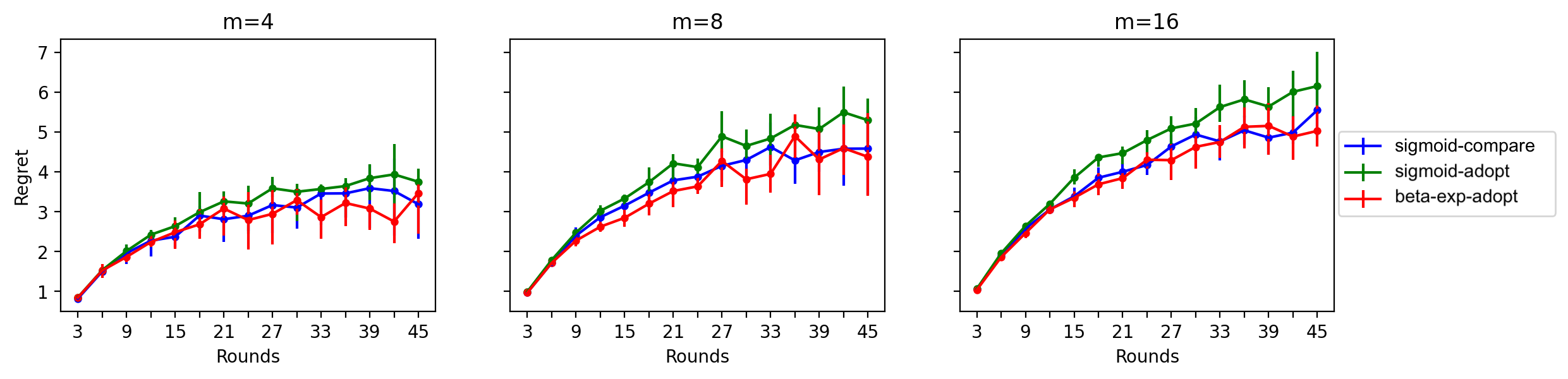
Figure 1: In the stationary setting with fixed-mean Bernoulli rewards: average regrets over $T$ rounds on populations of $n=16000$ and increasing number of actions $m$, for the three algorithms. Each regret value is averaged over 15 random iterations, and the error bars show the first and third quartiles over these iterations. The regret of each algorithm grows sublinearly in $T$, but it increases with $m$. Each algorithm was initialized from $\mathbf{p}=\mathbf{1}/m$.

We also examined the opposite scenario, where $m=4$ is fixed, but where the population size $n$ increases ($n\in\{400,4000,40000\}$). For this, we again considered a set of fixed-mean Bernoulli reward distributions, with means evenly-spaced between $0.85$ and $0.25$. For each algorithm, we used the same parameter settings as above, and again considered average regrets over the 15 iterations of each combination of algorithm, population size $n$, and rounds $T$. The results of these simulations are shown in Figure 2.

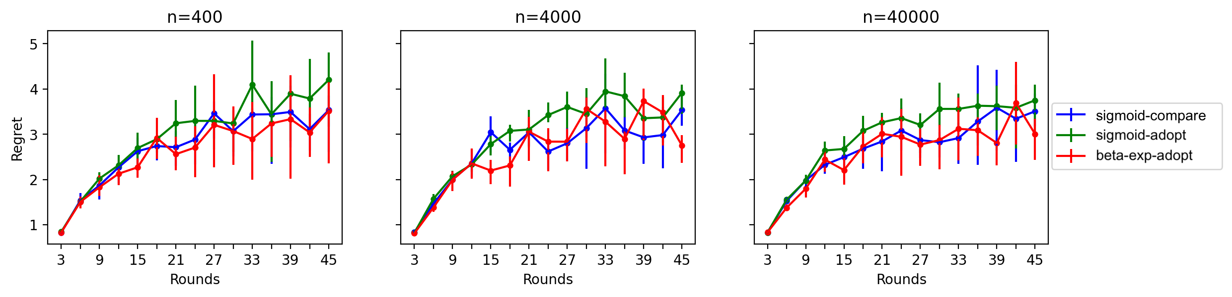
Figure 2: In the stationary setting with fixed-mean Bernoulli rewards: average regrets over $T$ rounds for increasing population sizes $n$ with a fixed number of actions $m=4$. Each regret value is averaged over 15 random iterations, and the error bars show the first and third quartiles over these iterations. Again, the regrets grows sublinearly in $T$, and we notice a slight dampening with larger $n$. Each algorithm was initialized from $\mathbf{p}=\mathbf{1}/m$.

Similar to Figure 1, in Figure 2 we observe in general that the average regret of each algorithm grows sublinearly over rounds at every population size. Although more subtle, we notice a slight downward trend in regret as the population size increases, which reinforces our intuition from Theorem 2.8. However, note from the theorem that for larger $n$, and $T\leq\sqrt{n}$, the (average) regret will be dominated by the $(\log m)/T$ approximation error term. Thus further increases to $n$ may lead to only negligible decreases in the overall regret if the estimation error is already small.

A.2 “Last Iterate Convergence” in the Stationary Reward Setting

We also experimentally examined the last iterate convergence properties of our algorithms in the stationary setting. This refers to an algorithm inducing a sequence of distributions $\{\mathbf{p}^{t}\}$ that converges (almost surely) to a point mass on the coordinate corresponding to the highest-mean action. This would imply that the regret of every subsequent round is 0. In the bandit literature, this behavior is sometimes referred to as best-arm identification (Lattimore & Szepesvári, 2020).

In Figure 3, we examine this by tracking the evolution of the distributions $\{\mathbf{p}^{t}\}$ in one random run of each of the $\beta$-$\mathsf{softmax}\text{-}\mathsf{compare}$, $\beta$-$\mathsf{sigmoid}\text{-}\mathsf{adopt}$, and $\beta$-$\mathsf{exp}\text{-}\mathsf{adopt}$ algorithms on a fixed reward sequence. For this, we considered the same set of $m=8$ fixed-mean Bernoulli distributions and the same $\beta$ parameters for each algorithm as described above. For each algorithm, we observe that the mass $p^{t}_{1}$ (corresponding to the action with highest mean reward) tends toward 1 after sufficiently many rounds, and thus our algorithm do seem to exhibit such last-iterate convergence behavior in this reward setting.

We remark that the prior work of Su et al. (2019) showed (in a slightly different model) that a similar family of processes results in such best-arm-identification with high probability when taking $T\to\infty$. However, given the behavior shown in Figure 3, investigating the conditions (i.e., the exact reward distribution structure) under which quantitative convergence rates for this beahvior can be established would be an interesting line of future work.

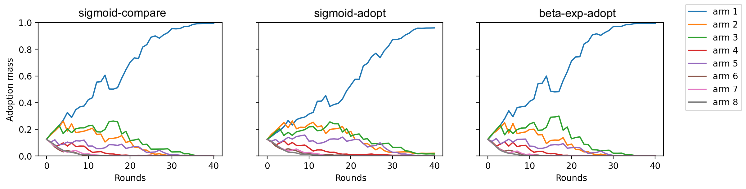
Figure 3: In the stationary setting with fixed-mean Bernoulli rewards: the evolution of the distributions $\{\mathbf{p}^{t}\}$ for each algorithm on one random run with $n=1600$ and an $m=8$ total actions. For each algorithm, the mass corresponding to the first action (with highest mean reward) appproaches 1 after around 30 rounds, which highlights a “last iterate convergence” phenomenon induced by our algorithms in the stationary setting. Each algorithm was initialized from $\mathbf{p}=\mathbf{1}/m$.

A.3 Convex Optimization Error in the Adversarial Reward Setting

To evaluate our algorithms in an adversarial reward setting, we simulated both the $\beta$-$\mathsf{softmax}\text{-}\mathsf{compare}$ and $\beta$-$\mathsf{sigmoid}\text{-}\mathsf{adopt}$ algorithms for a convex optimization task using the reward generation setup of Assumption 2 from Section 2.5. For this, we considered minimizing a three-dimensional convex function $f:\Delta_{3}\to\mathbb{R}$ given by

$$f(\mathbf{p})\;=\;\tfrac{3}{5}p_{1}^{2}+\tfrac{3}{10}p_{2}^{2}-\tfrac{5}{6}p_{1}+\tfrac{1}{15}p_{3}+\tfrac{44}{15}\;,$$ (7)

for $\mathbf{p}\in\Delta_{3}$. It is straightforward to verify that $f$ has gradients bounded by 1 over the simplex, and that $\mathbf{p}^{\star}:=(\tfrac{3}{4},\tfrac{1}{9},\tfrac{5}{36})$ minimizes $f$. We thus considered reward distributions of the form $\mathbf{g}^{t}=-\nabla f(\mathbf{p}^{t})+\mathbf{b}^{t}$, where each $\mathbf{b}^{t}$ has i.i.d. zero-mean Gaussian coordinates with variance $\sigma^{2}$, and clipped in the range $[-10,10]$.

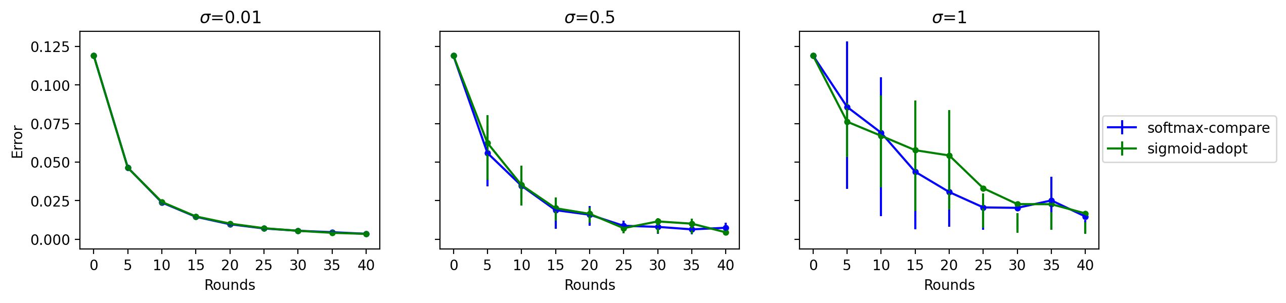
Figure 4: In the adversarial setting with reward distributions generated via a stochastic gradient oracle: optimization error of the function $f:\Delta_{3}\to\mathbb{R}$ (expression (7)) induced by the $\beta$-$\mathsf{softmax}\text{-}\mathsf{compare}$ and $\beta$-$\mathsf{sigmoid}\text{-}\mathsf{adopt}$ algorithms on a population of $n=3000$, initialized from the distribution $\mathbf{p}=\mathbf{1}/3$, and for increasingly noisy gradient oracles (larger $\sigma$). The error of both protocols after $T$ rounds is averaged over 15 iterations, and the error bars show the first and third quartiles. We notice that the optimization error approaches 0 for both algorithms after enough rounds, but this convergence is slower with larger $\sigma$.

In Figure 4, we show the function error between $\mathbf{p}^{\star}$ and the average iterate $\widetilde{\mathbf{p}}=\frac{1}{T}\sum_{t\in[T]}\mathbf{p}^{t}$ induced by the $\beta$-$\mathsf{softmax}\text{-}\mathsf{compare}$ and $\beta$-$\mathsf{sigmoid}\text{-}\mathsf{adopt}$ algorithms for this optimization task over increasing magnitudes of $\sigma$, and on a population of size $n=3000$. Similar to the previous plots, at each combination of protocol, $\sigma$, and $T$, we take the average error over 15 iterations of the process, and the error bars show the range of the first and third quartiles over these iterations.

Notice in each subplot that the error of both algorithms goes to 0 with the number of rounds, which highlights the robustness of our algorithms to reward sequences whose means vary over time. However, as expected, this error tends to increase for larger $\sigma$ (given that this corresponds to noisier stochastic gradients). This aligns with the inutition from the expected error rate of Theorem 2.10 in this setting.

Appendix B Related Work

In this section, we provide a more detailed discussion and comparison with several related works. As mentioned in the introduction, many distinct online learning and multi-agent bandit settings have been studied under various communication and coordination constraints (e.g., including (Lai et al., 2008; Liu & Zhao, 2010; Anandkumar et al., 2011; Hillel et al., 2013; Szorenyi et al., 2013; Avner & Mannor, 2014; Boursier & Perchet, 2019; Martínez-Rubio et al., 2019; He et al., 2019; cesa2020cooperative; Bubeck & Budzinski, 2020; Zhu et al., 2023). However, the problem setting of the present work can be viewed most directly as the (complete communication graph) GOSSIP-model analogue of the full-neighbor-communication cooperative bandit setting, which was studied previously (for general communication graphs $G$) in both stationary (e.g., (Szorenyi et al., 2013; Landgren et al., 2016; Kolla et al., 2018; Martínez-Rubio et al., 2019)) and adversarial reward setttings (e.g., (Awerbuch & Kleinberg, 2008; Cesa-Bianchi et al., 2016; Bar-On & Mansour, 2019)). By virtue of considering the all-to-all LOCAL communication model (Linial, 1992; Suomela, 2013) with a focus on general (non-complete) communication graphs, and without considering and decentralization constraints, the techniques of these prior works differ significantly from ours, and the results are not directly comparable.

On the other hand, the works of Celis et al. (2017), Su et al. (2019), and Sankararaman et al. (2019), do consider model variants and settings more closely related to the present work, and we provide some more detailed technical comparisons in the subsequent sections. Futher below, we also mention some connections between our families of local algorithms, and other other distributed consensus, opinion, and evolutionary game dynamics.

B.1 Comparison with Celis et al. (2017)

As mentioned in Section 1, Celis et al. considered a related distributed bandit model: they assume of population of $n$ agents and an $m$-armed bandit instance, where the rewards are generated from fixed-mean Bernoulli distributions, and where agents utilize a two-step uniform neighbor sampling and arm adoption process in each round. Specifically, they assume the following steps:

1. At round $t$, each agent either (a) with probability $(1-\mu)$ samples a uniformly random neighbor and observes its most recent adoption choice and reward, or (b) with probability $\mu>0$ selects an arm uniformly at random and observes its most recently generated reward.

2. Given the reward $g^{t}_{c}$ observed by an agent in the previous step, that agent adopts arm $c\in[m]$ in the subsequent round with probability $\beta^{g^{t}_{c}}\cdot(1-\beta)^{1-g^{t}_{c}}$, and otherwise makes no arm adoption.

We make several remarks on this process and how it relates to our own model and algorithms. First, note that by definition of this process, at any given round an agent will make no adoption choice with some non-zero probability. On the other hand, the authors assume that each arm-adoption distribution $\mathbf{p}^{t}$ is computed by normalizing with respect to the set of nodes that do make an adoption in round $t$.

However, their analysis relies on the assumption that, in step (i.a) above, an agent samples a neighbor that previously adopted arm $j$ with probability $p^{t}_{j}$. Note that this implies that the uniform neighbor sampling (with probability $1-\mu$) is only uniform over the set of neighbors in the population that made an adoption decision in the previous round. This could be implemented, for example, by a central coordinator that can generate samples from this subset of the population. However, it cannot be performed in a purely decentralized fashion in which each agent selects a neighbor uniformly at random, as in the GOSSIP model setting we consider. Thus the exact model considered by Celis et al. differs from the one described in Section 1, and this precludes a direct comparison of their results with ours.

On the other hand, we remark that the adoption probability expression in step (ii) above is similar of the $\beta$-$\mathsf{exp}\text{-}\mathsf{adopt}$ algorithm from Section 2, and their process was the inspiration for that specific instantiation of an adoption algorithm. However, the process of Celis et al. includes the additional component in step (i) of allowing each agent with probability $\mu>0$ to, rather than receiving information from a random neighbor, observe the most recent reward of an arm selected uniformly at random. In their analysis, this small non-negative probability is used to establish an adoption mass lower bound for the optimal arm in the stationary, Bernoulli reward setting.

We note that this uniform arm sampling can be advantageous in reducing the likelihood that the sequence of distributions $\{\mathbf{p}^{t}\}$ converges to a “fixed-point” sub-optimal arm decision. However, this same mechanism can also slow down convergence (or slightly increase regret) when a sufficiently large majority of the population mass is already accumulated at the coordinate of the highest-mean arm, and it also assumes agents have local memory of size linear in $m$. Thus, an interesting line of future work would be to better quantify the exact tradeoffs between algorithms that use such uniform arm-sampling mechanisms (as in the work Celis et al.), and algorithms that do not (as in the present work).

B.2 Comparisons with Su et al. (2019) and Sankararaman et al. (2019)

We also make some comparisons with the works of Su et al. (2019) and Sankararaman et al. (2019), although the exact settings in those are less similar than that of Celis et al. to the present paper.

The key similarity with our work is that communication between nodes occurs in a pairwise manner, but both works consider a related asynchronous gossip model (Boyd et al., 2006), where individual communications occur according to the arrivals of a Poisson clock with rate $n$. Note in expectation that $n$ total communications occur per time unit in this model, and thus it can be viewed as the natural, continuous time analog of the discrete-time, synchronous model in the present work.

However, besides from the similarity in pairwise agent communication, the bandit settings and problem objective of both works vary from ours. Su et al. consider fixed-mean Bernoulli reward distributions and are concerned mainly with the best arm identification task, which asks whether every agent will eventually adopt the highest-mean arm in perpetuity (note that the authors refer to this in their work as learnability). Nevertheless, the dynamics proposed by Su et al. can be viewed similarly to an instantiation of an adoption algorithm from Section 2, but their main result quantifies the probability that the population eventually identifies the highest-mean arm, rather than deriving a quantitative bound on the population-level regret achieved by their protocol.

On the other hand, the results of Su et al. apply to more general, non-complete communication graphs (that are sufficiently well-connected). Their results thus motivate the question of whether the algorithms and regret bounds of the present paper also transfer to non-complete graph topologies.

Similar to Su et al., Sankararaman et al. also consider Bernoulli reward distributions with fixed means, but they also assume that agents generate independent samples from the arm distributions upon each agent’s individual pulls. In this sense, the total number of independent arm pulls across the population per time unit can be as large as $n$ in expectation. This model difference is also reflected in their regret objective, which is to minimize the individual cumulative regrets aggregated across all agents in the population. In contrast, our results consider a population-level regret defined with respect to the global arm adoption distributions. The authors also assume that agents have the ability to remember their full history of previous adoption choices and observed rewards, and this allows for designing local algoritihms that adapt classic UCB approaches from centralized bandit settings (Lattimore & Szepesvári, 2020; Bubeck et al., 2012).

However, a key constraint in the algorithms proposed by Sankararaman et al. is that upon agent communications, nodes can exchange only the index of an action (rather than any recently observed rewards from that action) and in general, the authors are concerned with limiting the total number of per-agent communications over rounds. This motivates the question of whether the algorithms of the present paper can be adapted to only consider action index information, and to study the resulting impact on regret. This could be of interest in systems where agents can only communicate a limited number of bits, and thus communicating previously observed rewards to full precision is infeasible.

B.3 Relation to Consensus and Opinion Dynamics and Evolutionary Game Dynamics

We remark that our families of algorithms (particularly for the stationary reward setting) are more generally related to distributed consensus and opinion dynamics, which have been studied extensively in both synchronous and asynchronous GOSSIP-based models  (Doerr et al., 2011; Ghaffari & Lengler, 2018; Becchetti et al., 2014b; a; 2020; Amir et al., 2023). In these settings, the goal of the population is to eventually agree on one of $m$ opinions, and local interaction rules that involve an agent adopting (or refraining from adopting) the opinion of its randomly sampled neighbor (i.e., similar in spirit to our adoption and comparison algorithms) are usually at the foundation of such dynamics (Becchetti et al., 2014a; Amir et al., 2023).

Our algorithms are also related to evolutionary game dynamics on graphs (Allen & Nowak, 2014; Czyzowicz et al., 2015; Schmid et al., 2019). In these settings, one usually considers $m$ strategies, and each agent maintains one such strategy in each time step. Interactions between agents then correspond to two-player games, where each agent plays according to its current strategy and receives some reward according to a fixed payoff matrix. In general, dynamics in this setting allow better strategies to reproduce (more agents adopt these strategies), and for less-optimal strategies to become extinct. Here, the focus is usually on characterizing the various stability and equilibria properties achieved by such processes. The adoption and comparison algorithms from the present work can be viewed as similar evolutionary game processes, especially given the earlier-mentioned similarity between zero-sum MWU processes and the classical replicator dynamics (Schuster & Sigmund, 1983; Cabrales, 2000).

Establishing a more rigorous and quantitative relationship between algorithms for this decentalized bandit setting and previously studied consensus and evolutionary game dynamics in related gossip models is thus left as future work.

Appendix C Details on Evolution of Local Algorithms

In this appendix, we derive the conditionally expected evolution of the adoption algorithms (Appendix C.1) and comparison algorithms (Appendix C.2) that were introduced in Section 2. Then, in Appendix C.3, we also introduce a third family of two-neighbor comparison algorithms that generalizes comparison algorithms to a setting in which each agent samples two neighbors at every round. We show this family also yields a similar form of zero-sum multiplicative updates in conditional expectation.

Recall in this work that we consider a complete communication graph. We assume further this communication graph contains self-loops, which is a standard assumption in the GOSSIP model (Boyd et al., 2006; Shah et al., 2009; Becchetti et al., 2014a; 2020). Moreover, we use the terminlogy “the neighbor sampled by an agent $u$” to refer to the uniformly random neighbor that agent $u$ exchanges information with under the GOSSIP-style communication of the problem setting. However, we remark these random information exchanges should be viewed as being “scheduled” by the model. In other words, in the GOSSIP model, the agent $u$ does not explicitly pefform the neighbor sampling itself, but rather the model stipulates that in each round, every agent $u$ has a (one-sided) information exchange with a uniformly random neighbor.

C.1 Evolution of Adoption Dyanmics

For adoption dynamics, we provide the proof of Proposition 2.1, which is restated for convenience:

See 2.1

Proof.

First, letting $c^{t+1}_{u}\in[m]$ denote the action chosen by agent $u\in[n]$ in round $t+1$, observe that

$$\mathbb{E}_{t}[p^{t+1}_{j}]\;=\;\frac{1}{n}\sum_{u\in[n]}\mathbb{P}_{t}[c^{t+1}_{u}=j]\;,$$

which follows from the fact that $p^{t+1}_{j}$ is the average of the $n$ indicators $\mathbf{1}\{c^{t+1}_{u}=j\}$. By the local symmetry of the algorithm and communication model, $\mathbb{P}_{t}[c^{t+1}_{u}=j]$ is identical for all agents $u$. However, this value is dependent on $c^{t}_{u}$ (i.e., the action choice of $u$ at the previous round $t$).

Thus using the law of total probability, for any agent $u$ we can write

$$\mathbb{P}_{t}[c^{t+1}_{u}=j]\;=\;\mathbf{1}\{ c^{t}_{u}=j\}\cdot\mathbb{P}_{t}[c^{t+1}_{u}=j|c^{t}_{u}=j]$$

$$+\sum_{k\neq j\in[m]}\mathbf{1}\{c^{t}_{u}=k\}\cdot\mathbb{P}_{t}[c^{t+1}_{u}=j|c^{t}_{u}=k]\;.$$

Now fix agent $u$, and let $v\in[n]$ denote the agent that $u$ samples in round $t$. Now recall from the definition of the algorithm that if $c^{t}_{u}=k\neq j$, then $c^{t+1}_{u}=j$ with probability $f(g^{t}_{j})$ only if agent $v$ chose action $j$ in round $t$, i.e., $c^{t}_{v}=j$. On the other hand, if $c^{t}_{u}=j$, then $c^{t+1}_{u}=j$ either if $c^{t}_{v}=j$, or if $c^{t}_{v}=k\neq j$ and agent $u$ rejects adopting action $k$ with probability $1-f(g^{t}_{k})$.

Thus we have

$$\mathbb{P}_{t}[c^{t+1}_{u}=j|c^{t}_{u}=j] \;=\;p^{t}_{j}+\sum_{k\neq j\in[m]}p^{t}_{k}\cdot(1-f(g^{t}_{k}))$$

$$\text{and}\;\;\;\mathbb{P}_{t}[c^{t+1}_{u}=j|c^{t}_{u}=k] \;=\;p^{t}_{j}\cdot f(g^{t}_{j})\;\;\;\text{for $k\neq j$}\;.$$

Combining these cases, noting also that $\frac{1}{n}\sum_{u\in[v]}\mathbf{1}\{c^{t}_{u}=k\}=p^{t}_{k}$ for any $k\in[m]$, and using the fact that $\sum_{k\in[m]}p^{t}_{k}=1$, we can then write

$$\mathbb{E}_{t}[p^{t+1}_{j}] \;=\;p^{t}_{j}\cdot\big{(}p^{t}_{j}+\sum_{k\neq j\in[m]}p^{t}_{k}\cdot(1-f(g^{t}_{k}))\big{)}+\sum_{k\neq j\in[m]}p^{t}_{k}\cdot\big{(}p^{t}_{j}\cdot f(g^{t}_{j})\big{)}$$

$$\;=\;p^{t}_{j}\cdot\Big{(}1+\sum_{k\neq j\in[m]}p^{t}_{k}\cdot\big{(}f(g^{t}_{j})-f(g^{t}_{k})\big{)}\Big{)}$$

$$\;=\;p^{t}_{j}\cdot\Big{(}1+f(g^{t}_{j})-\big{\langle}\mathbf{p}^{t},f(\mathbf{g}^{t})\big{\rangle}\Big{)}\;,$$

which concludes the proof. ∎

Importantly, we also verify that such multiplicative updates in every coordinate $j$ still lead to a proper distribution: for this, it is easy to check that

$$\sum_{j\in[m]}\mathbb{E}_{t}[p^{t+1}_{j}] \;=\;\sum_{j\in[m]}p^{t}_{j}\cdot\Big{(}1+f(g^{t}_{j})-\big{\langle}\mathbf{p}^{t},f(\mathbf{g}^{t})\big{\rangle}\Big{)}$$

$$\;=\;\sum_{j\in[m]}p^{t}_{j}+\big{\langle}\mathbf{p}^{t},f(\mathbf{g}^{t})\big{\rangle}-\big{\langle}\mathbf{p}^{t},f(\mathbf{g}^{t})\big{\rangle}\;=\;1\;,$$

which holds since $\mathbf{p}^{t}$ is a distribution.

Finally, recall from Section 2.1 that when the adoption function $f$ is a sigmoid function with parameter $\beta$ we call the resulting local algorithm $\beta$-$\mathsf{sigmoid}\text{-}\mathsf{adopt}$. Stated formally:

Local Algorithm 1.

Let $\beta$-$\mathsf{sigmoid}\text{-}\mathsf{adopt}$ be the adoption algorithm instantiated by the function $f_{\beta}(g):=\frac{1}{1+\exp(-\beta\cdot g)}$ for $\beta\in[0,1]$ and any $g\in\mathbb{R}$.

Similarly, in the case when all rewards $\mathbf{g}^{t}$ are binary, and we have the following $\beta$-$\mathsf{exp}\text{-}\mathsf{adopt}$ algorithm:

Local Algorithm 2.

Let $\beta$-$\mathsf{exp}\text{-}\mathsf{adopt}$ be the adoption dynamics protocol instantiated by the adoption function $f_{\beta}(g):=\beta^{g}\cdot(1-\beta)^{1-g}$ for $\beta\in(0.5,1)$ and $g\in\{0,1\}$.

Finally, when all rewards $\mathbf{g}^{t}\in[0,\sigma]^{m}$, we have have the following $\beta$-$\mathsf{disc}\text{-}\mathsf{adopt}$ protocol:

Local Algorithm 3.

Let $\beta$-$\mathsf{disc}\text{-}\mathsf{adopt}$ be the adoption algorithm instantiated by the adoption function $f_{\beta}(g):=\beta\cdot g$ for $\beta\in(0,1/\sigma]$ when all $g\in[0,\sigma]$.

C.2 Evolution of Comparison Algorithms

For comparison algorithms, we develop the proof of Proposition 2.2, which is restated here:

See 2.2

Proof.

Fix $j\in[m]$ and $t\in[T]$. Again let $c^{t}_{i}\in[m]$ denote the action chosen by agent $i\in[n]$ at round $t$. Then observe that we can write

$$\mathbb{E}_{t}\big{[}p^{t+1}_{j}\big{]}\;=\;\frac{1}{n}\sum_{i\in[n]}\mathbb{P}_{t}\big{[}c^{t+1}_{i}=j\big{]}\;=\;\frac{1}{n}\sum_{i\in[n]} \Bigg{(}\mathbf{1}\{c^{t}_{i}=j\}\cdot\mathbb{P}_{t}\big{[}c^{t+1}_{i}=j\;|\;c^{t}_{i}=j\big{]}$$

$$+\sum_{k\neq j\in[m]}\mathbf{1}\{c^{t}_{i}=k\}\cdot\mathbb{P}_{t}\big{[}c^{t+1}_{i}=j\;|\;c^{t}_{i}=k\big{]}\Bigg{)}\;.$$

In the case that $c^{t}_{i}=j$, note that $c^{t+1}=j$ with probability 1 if agent $i$ samples an agent $u$ that also chose action $j$ in round $t$. Otherwise, if agent $u$ chose some action $k\neq j$, then agent $i$ chooses action $j$ with probability $1-h(g^{t}_{k})/\big{(}h(g^{t}_{j})+h(g^{t}_{k})\big{)}$. Together, this means that

$$\mathbb{P}_{t}\Big{[}c^{t+1}_{i}=j\;|\;c^{t}_{i}=j\Big{]} \;=\;p^{t}_{j}+\sum_{k\neq j\in[m]}p^{t}_{k}\Bigg{(}1-\frac{h(g^{t}_{k})}{h(g^{t}_{j})+h(g^{t}_{k})}\Bigg{)}$$

$$\;=\;1-\sum_{k\neq j\in[m]}p^{t}_{k}\cdot\frac{h(g^{t}_{k})}{h(g^{t}_{j})+h(g^{t}_{k})}\;\;\;.$$ (8)

In the other case when $c^{t}_{i}=k\neq j$, then $c^{t+1}=j$ only when agent $i$ samples a neighbor that chose action $j$ in round $t$, and thus

$$\mathbb{P}_{t}\big{[}c^{t+1}_{i}=j\;|\;c^{t}_{i}=k\big{]}\;=\;p^{t}_{j}\cdot\frac{h(g^{t}_{j})}{h(g^{t}_{j})+h(g^{t}_{k})}\;.$$ (9)

Now observe that for any $k\in[m]$, $\tfrac{1}{n}\sum_{i\in[n]}\mathbf{1}\{c^{t}_{i}=k\}=p^{t}_{k}$ by definition. Then together with expression (8) and (9), we have

$$\mathbb{E}_{t}\big{[}p^{t+1}_{j}\big{]} \;=\;p^{t}_{j}\Bigg{(}1-\sum_{k\neq j\in[m]}p^{t}_{k}\cdot\frac{h(g^{t}_{k})}{h(g^{t}_{j})+h(g^{t}_{k})}\Bigg{)}+\sum_{k\neq j\in[m]}p^{t}_{k}\cdot p^{t}_{j}\frac{h(g^{t}_{j})}{h(g^{t}_{j})+h(g^{t}_{k})}$$

$$\;=\;p^{t}_{j}\cdot\Bigg{[}1+\sum_{k\neq j\in[m]}p^{t}_{k}\cdot\frac{h(g^{t}_{j})-h(g^{t}_{k})}{h(g^{t}_{j})+h(g^{t}_{k})}\Bigg{]}$$

$$\;=\;p^{t}_{j}\cdot\Big{[}1+\big{\langle}\mathbf{p}^{t},H(\mathbf{g}^{t},j)\big{\rangle}\Big{]}\;,$$

which concludes the proof. ∎

Again, we also verify that for any $\mathbf{p}\in\Delta_{m}$ and $\mathbf{g}\in[0,1]^{m}$, the family of functions $\{\langle\mathbf{p},H(\mathbf{g},j)\rangle\}_{j\in[m]}$ satisfies the zero-sum property $\sum_{j\in[m]}p_{j}\cdot\langle\mathbf{p},H(\mathbf{g},j)\rangle=0$. To see this, observe that

$$\sum_{j\in[m]}p_{j}\cdot\langle\mathbf{p},H(\mathbf{g},j)\rangle \;=\;\sum_{j\in[m]}p_{j}\cdot\sum_{k\in[m]}p_{k}\cdot\frac{h(g^{t}_{j})-h(g^{t}_{k})}{h(g^{t}_{j})+h(g^{t}_{k})}$$

$$\;=\;\sum_{(j,k)\in[m]\times[m]}p_{j}\cdot p_{k}\cdot\Bigg{(}\frac{h(g^{t}_{j})-h(g^{t}_{k})}{h(g^{t}_{j})+h(g^{t}_{k})}+\frac{h(g^{t}_{k})-h(g^{t}_{j})}{h(g^{t}_{j})+h(g^{t}_{k})}\Bigg{)}\;=\;0\;.$$

Finally, recall that when the score function $h$ is an exponential with parameter $\beta$, we call the resulting algorithm $\beta$-$\mathsf{softmax}\text{-}\mathsf{compare}$. Defined formally:

Local Algorithm 4 ($\beta$-softmax-comparison).

Let $\beta$-$\mathsf{softmax}\text{-}\mathsf{compare}$ denote the comparison algorithm instantiated with the score function $h_{\beta}(g):=\exp(\beta\cdot g)$ for some $\beta\in[0,1]$.

C.3 Two-Neighbor Comparison Algorithms

We now introduce a third family of algorithms that assumes a slight generalization on the model specified in Section 1. In particular, we now suppose in step (ii) of the model that each agent $u$ can receive information from two randomly sampled neighbors. Agent $u$ can then incorporate the most recent action choice and reward of both neighbors to determine its own decision in the next round. This communication assumption can be viewed as a 2-neighbor GOSSIP model variant.

With this model variation, we state a family of natural two-neighbor comparison algorithms. For this, let $h:\mathbb{R}\to\mathbb{R}_{\geq 0}$ be a non-decreasing score function applied to a reward $\mathbf{g}\in\mathbb{R}$. Given $h$, these algorithms (stated from the perspective of any fixed agent $u\in[n]$ at round $t+1$ of the process) proceed as follows:

Two-Neighbor Comparison Algorithms: Given a non-decreasing score function $h:\mathbb{R}\to\mathbb{R}_{\geq 0}$, for each $u\in[n]$: (i) At round $t$, assume: agent $u$ chose action $j$; $u$ sampled agents $v\in[n]$ and $w\in[n]$; and agent $v$ chose action $k\in[m]$, and agent $w$ chose action $\ell\in[m]$. (ii) At round $t+1$: for $c\in\{j,k,\ell\}$, define $\rho_{c}=\frac{h\big{(}g^{t}_{c}\big{)}}{\sum_{b\in\{j,k,\ell\}}h\big{(}g^{t}_{b}\big{)}}$.
Then agent $u$ chooses action $c\in\{j,k,\ell\}$ with probability $\rho_{c}$.

In other words, these algorithms simply extend the logic of (single-neighbor) comparison algorithms to the case when each agent samples information from two neighbors. Similar to the adoption and comparison algorithms from above, we again show that under these algorithms, the coordinate-wise evolution of the distribution $\mathbf{p}^{t}$ takes on a “zero-sum” form in conditional expectation:

Lemma C.1.

Let $\{\mathbf{p}^{t}\}$ be the sequence induced by running any two-neighbor comparison algorithms with score function $h$ and reward sequence $\{\mathbf{g}^{t}\}$. Furthermore, for any $\mathbf{g}\in\mathbb{R}^{m}$ and each $j\in[m]$, let $\mathbf{H}_{j}(\mathbf{g})\in\mathbb{R}^{m\times m}$ be the symmetric matrix whose entries are specified by:

$$\mathbf{H}_{j}(\mathbf{g})_{j,j} \;=\;0$$

$$\mathbf{H}_{j}(\mathbf{g})_{k,k} \;=\;\frac{2(h(g_{j})-h(g_{k}))}{h(g_{j})+2h(g_{k})}\;\;\;\text{for $k\neq j\in[m]$}$$

$$\mathbf{H}_{j}(\mathbf{g})_{j,k} \;=\;\frac{h(g_{j})-h(g_{k}))}{2h(g_{j})+h(g_{k})}\;\;\;\text{for $k\neq j\in[m]$}$$

$$\text{and}\;\;\;\mathbf{H}_{j}(\mathbf{g})_{k,\ell} \;=\;\frac{h(g_{j})-(h(g_{k})+h(g_{\ell}))}{h(g_{j})+h(g_{k})h(g_{\ell})}\;\;\;\;\text{for $k\neq\ell\neq j\in[m]$}\;.$$

Then for all $t\in[T]$:

$$\mathbb{E}_{t}\big{[}p^{t+1}_{j}\big{]}\;=\;p^{t}_{j}\cdot\Big{(}1+\big{\langle}\mathbf{p}^{t},\mathbf{H}_{j}(\mathbf{g}^{t})\;\mathbf{p}^{t}\big{\rangle}\Big{)}\;.$$

Proof.

The proof of the lemma follows similarly to those of Lemmas 2.1 and 2.2, but with more cases to handle the two-neighbor sampling. Again, we write $c^{t}_{u}\in[m]$ to denote the action chosen by a agent $u\in[n]$ at round $t\in[T]$, and again our strategy is to compute $\mathbb{P}_{t}[c^{t+1}_{i}=j]$ in two cases: (i) when $c^{t}_{i}=j$, and when $c^{t}_{i}=k\neq j$.

For the first case, when $c^{t}_{i}=j$, consider the following combinations of neighbor sampling outcomes (at round $t$) and action choice probabilities that could result in agent $i\in[n]$ (re)choosing action $j$:

1. Agent $i$ samples two neighbors that both chose action $j$ in round $t$, which occurs with probability $(p^{t}_{j})^{2}$. Then agent $i$ subsequently chooses action $j$ in round $t+1$ with probability 1.

2. Agent $i$ samples two neighbors that both chose action $k\neq j\in[m]$, which occurs with probability $(p^{t}_{k})^{2}$. Then agent $i$ subsequently chooses action $j$ with probabiltiy $1-h(g^{t}_{k})/(h(g^{t}_{j})+2h(g^{t}_{k}))$.

3. Agent $i$ samples one neighbor that chose action $j$, and one that chose action $k\neq j$, which occurs with probability $2p^{t}_{j}p^{t}_{k}$. Then agent $i$ subsequently chooses action $j$ with probability $1-h(g^{t}_{k})/(2h(g^{t}_{j})+h(g^{t}_{k}))$.

4. Agent $i$ samples two neighbors that chose actions $k\neq j$ and $\ell\neq k\neq j$ respectively, which occurs with probability $p^{t}_{k}p^{t}_{\ell}$. Then agent $i$ subsequently chooses action $j$ with probability $1-(h(g^{t}_{k})+h(g^{t}_{\ell}))/(h(g^{t}_{j})+h(g^{t}_{k})+h(g^{t}_{\ell}))$.

Then combining each of these three cases means that

$$\mathbb{P}_{t}[c^{t+1}_{i}=j|c^{t}_{i}=j]\;=\;(p^{t}_{j})^{2} +\sum_{k\neq j\in[m]}(p^{t}_{k})^{2}\cdot\Big{(}1-\frac{2h(g^{t}_{k})}{h(g^{t}_{j})+2h(g^{t}_{k})}\Big{)}$$

$$+\sum_{k\neq j\in[m]}2p^{t}_{k}p^{t}_{j}\cdot\Big{(}1-\frac{h(g^{t}_{k})}{2h(g^{t}_{j})+h(g^{t}_{k})}\Big{)}$$

$$+\sum_{(k,\ell);k\neq\ell\neq j\in[m]}2p^{t}_{k}p^{t}_{\ell}\cdot\Big{(}1-\frac{h(g^{t}_{k})+h(g^{t}_{\ell})}{h(g^{t}_{j})+h(g^{t}_{k})+h(g^{t}_{\ell})}\Big{)}\;.$$

Now we consider a similar decomposition in the case when $c^{t}_{i}=k\neq j$:

1. Agent $i$ samples two agents that both chose action $j$ in round $t$ with probability $(p^{t}_{j})^{2}$, and agent $i$ subsequently re-chooses action $j$ with probability $2h(g^{t}_{j})/(2h(g^{t}_{j})+h(g^{t}_{k}))$.

2. Agent $i$ samples one neighbor that chose action $j$, and another neighbor that chose action $k$ with probability $2p^{t}_{j}p^{t}_{k}$. Then agent $i$ subsequently chooses action $j$ with probability $h(g^{t}_{j})/(h(g^{t}_{j})+2h(g^{t}_{k}))$.

3. Agent $i$ samples one neighbor that chose action $j$ and one neighbor that chose action $\ell\neq k\neq j\in[m]$ with probability $2p^{t}_{j}p^{t}_{\ell}$. Then agent $i$ subsequently chooses action $j$ with probability $h(g^{t}_{j})/(h(g^{t}_{j})+h(g^{t}_{k})+h(g^{t}_{\ell}))$.

Using these scenarios, we can then compute for each $k\neq j\in[m]$:

$$\mathbb{P}_{t}[c^{t+1}_{i}=j|c^{t}_{i}=k]\;=\;(p^{t}_{j})^{2}\cdot\frac{2h(g^{t}_{j})}{2h(g^{t}_{j})+h(g^{t}_{k})} +2p^{t}_{j}p^{t}_{k}\cdot\frac{h(g^{t}_{j})}{h(g^{t}_{j})+2h(g^{t}_{k})}$$

$$+\sum_{\ell\neq k\neq j\in[m]}2p^{t}_{j}p^{t}_{\ell}\cdot\frac{h(g^{t}_{j})}{h(g^{t}_{j})+h(g^{t}_{k})+h(g^{t}_{\ell})}\;.$$

Then in the multplying by $p^{t}_{j}$ in the first case, and summing over $p^{t}_{k}\cdot\mathbb{P}_{t}[c^{t+1}_{i}=j|c^{t}_{i}=k]$ for each $k\neq j\in[m]$ in the second case (which converts the conditional probabilities into joint expectations), and adding the two expressions and simplifying gives

$$\mathbb{E}_{t}[c^{t+1}_{i}=j]\;=\;p^{t}_{j}\cdot\Bigg{(}\bigg{(}\sum_{k\in[m]}p^{t}_{k}\bigg{)}^{2} +\sum_{k\neq j\in[m]}2p^{t}_{k}p^{t}_{j}\cdot\bigg{(}\frac{h(g^{t}_{j})-h(g^{t}_{k})}{2h(g^{t}_{j})+h(g^{t}_{k})}\bigg{)}$$

$$+\sum_{k\neq j\in[m]}(p^{t}_{k})^{2}\cdot\bigg{(}\frac{2h(g^{t}_{j})-2h(g^{t}_{k})}{h(g^{t}_{j})+2h(g^{t}_{k})}\bigg{)}$$

$$+\sum_{(k,\ell);k\neq\ell\neq j\in[m]}2p^{t}_{k}p^{t}_{\ell}\cdot\bigg{(}\frac{h(g^{t}_{j})-(h(g^{t}_{k})+h(g^{t}_{\ell}))}{h(g^{t}_{j})+h(g^{t}_{k})+h(g^{t}_{\ell})}\bigg{)}\Bigg{)}\;,$$

where we used the binomial theorem to simplify and extract the the term $\bigg{(}\sum_{k\in[m]}p^{t}_{k}\bigg{)}^{2}$, which is equal to 1 given that $\mathbf{p}^{t}$ is a distribution. Then using the summation form of a symmetric quadratic form, and using the definition of the entries of $\mathbf{H}_{j}(\mathbf{g})$ from the lemma statement, we can further simplify to write

$$\mathbb{P}_{t}[c^{t+1}_{i}=j]\;=\;p^{t}_{j}\cdot\Big{(}1+\big{\langle}\mathbf{p}^{t},\mathbf{H}_{j}(\mathbf{g})\mathbf{p}^{t}\big{\rangle}\Big{)}\;,$$

which concludes the proof. ∎

Appendix D Details on Zero-Sum Multiplicative Weights Update

In this section, we prove the regret bound on the zero-sum MWU process from Theorem 2.5, restated here:

See 2.5

For convenience, we also restate Assumption 1:

See 1

Roughly speaking, condition (i) of the assumption allows us to relate each $F_{j}(\mathbf{q},\mathbf{g})$ to $g_{j}$ in (conditional) expectation. From there, we can leverage standard approaches to proving MWU regret bounds (i.e., in the spirit of Arora et al. (2012)), but with some additional bookkeeping to account for the $\alpha_{1},\alpha_{2}$, and $\delta$ parameters. In the stationary reward setting and assuming $\delta=0$, we can further use the fact that $\mu_{1}\geq\langle\mathbf{p}^{t},\boldsymbol{\mu}\rangle$ for all rounds $t$ to derive a much smaller cumulative regret bound that is only a constant with respect to $T$. We also allow for a probabilistic lower bound on the initial mass at the $j$’th coordinate, which is useful for deriving the epoch-based regret bounds from Section 2.4.

Proof (of Theorem 2.5).

Fix $j\in[m]$ and $t\in[T]$. Recall that in round $t$, both $\mathbf{q}^{t}$ and $\mathbf{g}^{t}$ are random variables, where $\mathbf{q}^{t}$ depends on the randomness in both $\{\mathbf{q}^{t-1}\}$ and $\{\mathbf{g}^{t-1}\}$. Then conditioning on both of these sequences (which is captured in the notation $\mathbb{E}_{t-1}[\cdot]$), we can use the definition of the update rule in expression (3) to write

$$\mathbb{E}_{t-1}\big{[}q^{t}_{j}\big{]} \;=\;\mathbb{E}_{t-1}\big{[}\;q^{t}_{j}\cdot\big{(}1+F_{j}(\mathbf{q}^{t},\mathbf{g}^{t})\big{)}\;\big{]}$$

$$\;=\;q^{t}_{j}\cdot\mathbb{E}_{t-1}\big{[}1+F_{j}(\mathbf{q}^{t},\mathbf{g}^{t})\big{]}\;=\;q^{t}_{j}\cdot\big{(}1+\mathbb{E}_{t-1}\big{[}F_{j}(\mathbf{q}^{t},\mathbf{g}^{t})\big{]}\big{)}\;.$$

Here, the second equality comes from the fact that $\mathbf{q}^{t}$ is a constant when conditioning on $\{\mathbf{q}^{t-1}\}$ and $\{\mathbf{g}^{t-1}\}$, and thus $\mathbb{E}_{t-1}[q^{t}_{j}]=q^{t}_{j}$. Now for readability, let us define

$$m^{t}_{j}\;:=\;\mathbb{E}_{t-1}\big{[}F_{j}(\mathbf{q}^{t},\mathbf{g}^{t})\big{]}\;,$$

and that $m^{t}_{j}$ is deterministic (meaning $\mathbb{E}[m^{t}_{j}]=m^{t}_{j}$), since the only remaining randomness after the conditioning is with respect to $\mathbf{g}^{t}$. Thus using the law of iterated expectation, we can ultimately write

$$\mathbb{E}\big{[}q^{t+1}_{j}\big{]}\;=\;\mathbb{E}\big{[}\;\mathbb{E}_{t-1}\big{[}q^{t+1}_{j}\big{]}\;\big{]}\;=\;\mathbb{E}\big{[}q^{t}_{j}\big{]}\cdot\big{(}1+m^{t}_{j}\big{)}\;.$$

By repeating the preceding argument for each of $\mathbb{E}[q^{t-1}_{j}],\dots,\mathbb{E}[q^{1}_{j}]$, and setting $T=t+1$, we find that

$$\mathbb{E}\big{[}q^{T}_{j}\big{]}\;=\;q^{0}_{j}\cdot\prod_{t\in[T-1]}\big{(}1+m^{t}_{j}\big{)}\;.$$ (10)

From here, we roughly follow a standard multiplicative weights analysis: first, define the sets $M_{j}^{+}$ and $M_{j}^{-}$ as

$$M_{j}^{+} \;=\;\{t\in[T-1]\;:\;m^{t}_{j}\geq 0\}$$

$$\text{and}\;\;M_{j}^{-} \;=\;\{t\in[T-1]\;:\;m^{t}_{j}<0\}\;,$$

where clearly $M^{+}_{j}\cup M^{-}_{j}=[T]$. Then we can rewrite expression (10) as

$$\mathbb{E}[q^{T}_{j}]\;=\;q^{0}_{j}\cdot\prod_{t\in M^{+}_{j}}\big{(}1+m^{t}_{j}\big{)}\cdot\prod_{t\in M^{-}_{j}}\big{(}1+m^{t}_{j}\big{)}\;.$$

Now for each $t$, define $\Delta^{t}_{j}:=\mu^{t}_{j}-\langle\mathbf{q}^{t},\boldsymbol{\mu}^{t}\rangle\in[-2,2].$ Using this notation, observe that Assumption 1 implies

$$m^{t}_{j} \;\geq\;\frac{\alpha_{1}}{3}\cdot(\Delta^{t}_{j}-\delta)\;\;\;\text{when $m^{t}_{j}\geq 0$}$$

$$\text{and}\;\;\;m^{t}_{j} \;\geq\;\frac{\alpha_{2}}{3}\cdot(\Delta^{t}_{j}-\delta)\;\;\;\text{when $m^{t}_{j}<0$}\;.$$

Note that when $m^{t}_{j}<0$, the latter inequality implies that $\Delta^{t}_{j}-\delta<0$. On the other hand, when $m^{t}_{j}\geq 0$, the first inequality provides no further information on the sign of $\Delta^{t}_{j}-\delta$. Thus we define the additional two sets $G_{j}^{+}$ and $G_{j}^{-}$ as

$$G_{j}^{+} \;=\;\{t\in[T-1]\;:\;\Delta^{t}_{j}-\delta\geq 0\}$$

$$\text{and}\;\;G_{j}^{-} \;=\;\{t\in[T-1]\;:\;\Delta^{t}_{j}-\delta<0\}\;.$$

Combining the pieces above, it follows that

$$\mathbb{E}[q^{T}_{j}] \;\geq\;q^{0}_{j}\cdot\prod_{t\in M^{+}_{j}}\Big{(}1+\alpha_{1}\tfrac{(\Delta^{t}_{j}-\delta)}{3}\Big{)}\cdot\prod_{t\in M^{-}_{j}}\Big{(}1+\alpha_{2}\tfrac{(\Delta^{t}_{j}-\delta)}{3}\Big{)}$$

$$\;=\;q^{0}_{j}\cdot\prod_{t\in M^{+}_{j}\cap G^{+}_{j}}\Big{(}1+\alpha_{1}\tfrac{(\Delta^{t}_{j}-\delta)}{3}\Big{)}\cdot\prod_{t\in M^{+}_{j}\cap G^{-}_{j}}\Big{(}1+\alpha_{1}\tfrac{(\Delta^{t}_{j}-\delta)}{3}\Big{)}\cdot\prod_{t\in M^{-}_{j}}\Big{(}1+\alpha_{2}\tfrac{(\Delta^{t}_{j}-\delta)}{3}\Big{)}\;.$$

Observe also that each $|\Delta^{t}_{j}-\delta|\in[-3,3]$ by the definition of $\Delta^{t}_{j}$ and by the assumption that $\delta\in[0,1]$. Thus we can then use the facts that $(1+\alpha x)\geq(1+\alpha)^{x}$ for $x\in[0,1]$, and that $(1+\alpha x)\geq(1-\alpha)^{-x}$ for $x\in[-1,0$], which allows us to further simplify and write

$$\mathbb{E}[q^{T}_{j}]\;\geq\;q^{0}_{j}\cdot\prod_{t\in M^{+}_{j}\cap G^{+}_{j}}(1+\alpha_{1})^{\frac{(\Delta^{t}_{j}-\delta)}{3}}\cdot\prod_{t\in M^{+}_{j}\cap G^{-}_{j}}(1-\alpha_{1})^{-\frac{(\Delta^{t}_{j}-\delta)}{3}}\cdot\prod_{t\in M^{-}_{j}}(1-\alpha_{2})^{-\frac{(\Delta^{t}_{j}-\delta)}{3}}\;.$$

Now using the fact that $q^{T}_{j}\leq 1$, taking logarithms, and multiplying through by 3, we find

$$0\;\geq\;3\log q^{0}_{j}\;+ \sum_{t\in M^{+}_{j}\cap G^{+}_{j}}\log(1+\alpha_{1})(\Delta^{t}_{j}-\delta)$$

$$- \sum_{t\in M^{+}_{j}\cap G^{-}_{j}}\log(1-\alpha_{1})(\Delta^{t}_{j}-\delta)\;-\sum_{t\in M^{-}_{j}}\log(1-\alpha_{2})(\Delta^{t}_{j}-\delta)\;.$$ (11)

From here, we conclude the proof by considering the stationary and adversarial settings separately.

Stationary reward setting with $\delta=0$: We start with stationary reward setting and further assume $\delta=0$. Consider $j=1$, and observe by the assumption of on the ordering of coordinates in $\boldsymbol{\mu}$ that $\Delta^{t}_{1}=\mu_{1}-\langle\mathbf{q}^{t},\boldsymbol{\mu}\rangle\geq 0$ for all $\mathbf{q}^{t}$. Thus by definition, we have $M^{+}_{1}\cap G^{+}_{1}=T$, and expression (11) simplifies to

$$0\;\geq\;3\log q^{0}_{j}\;+\sum_{t\in[T]}\log(1+\alpha_{1})\Delta^{t}_{j}\;.$$

Using the identity $\log(1+x)\geq x-x^{2}\geq x/2$ (which holds for all $x\in(0,1/2)$) and rearranging terms then yields

$$\sum_{t\in[T]}\Delta^{t}_{1}\;\leq\;\frac{6\log(1/q^{0}_{j})}{\alpha_{1}}\;.$$ (12)

By definition, we have $\Delta^{t}_{1}=\mu_{1}-\langle\mathbf{q}^{t},\boldsymbol{\mu}\rangle$ for each $t$, and thus we can write $\langle\mathbf{q}^{t},\boldsymbol{\mu}\rangle=\langle\mathbf{q}^{t},\mathbb{E}[\mathbf{g}^{t}]\rangle=\mathbb{E}_{\mathbf{q}^{t}}[\langle\mathbf{q}^{t},\mathbf{g}^{t}\rangle]$. Moreover, by the assumption that $\mathbf{q}^{0}_{1}\geq\rho>0$ with probability at least $1-\gamma$, we have with this same probability that

$$T\cdot\mu_{1}-\sum_{t\in[T]}\mathbb{E}_{\mathbf{q}^{t}}[\langle\mathbf{q}^{t},\mathbf{p}^{t}\rangle]\;\leq\;\frac{6\log(1/q^{0}_{1})}{\alpha_{1}}\;.$$

Then taking expectations and using the law of iterated expectation, we have

$$\widetilde{R}(T,1)\;=\;T\cdot\mu_{1}-\sum_{t\in[T]}\mathbb{E}[\langle\mathbf{q}^{t},\mathbf{p}^{t}\rangle]\;\leq\;\frac{6\log(1/q^{0}_{1})}{\alpha_{1}}+\gamma\;,$$

which proves the claim for the stationary case.

General adversarial reward setting: We now consider the general adversarial reward setting and pick back up from expression (11). By definition, recall that $(\delta^{t}_{j}-\delta)$ is non-negative for $t\in M^{+}_{j}\cap G^{+}_{j}$, and negative for $t\in M^{+}_{j}\cap G^{-}_{j}$ and $t\in M^{-}_{j}$. Thus again using the identities $\log(1+x)\geq x-x^{2}$ and $-\log(1-x)\leq x+x^{2}$, which both hold for all $x\in[0,\tfrac{1}{2}]$, we can further bound expression (11) and rearrange to find

$$3 \log(1/q^{0}_{j})$$

$$\;\geq\;\sum_{t\in M^{+}_{j}\cap G^{+}_{j}}(\alpha_{1}-\alpha_{1}^{2})(\Delta^{t}_{j}-\delta)+\sum_{t\in M^{+}_{j}\cap G^{-}_{j}}(\alpha_{1}+\alpha_{1}^{2})(\Delta^{t}_{j}-\delta)+\sum_{t\in M^{-}_{j}}(\alpha_{2}+\alpha_{2}^{2})(\Delta^{t}_{j}-\delta)$$

$$\;=\;\sum_{t\in M^{+}_{j}\cap G^{+}_{j}}\Delta^{t}_{j}\alpha_{1}\;-\sum_{t\in M^{+}_{j}\cap G^{+}_{j}}\Delta^{t}_{j}\alpha_{1}^{2}\;-\sum_{t\in M^{+}_{j}\cap G^{+}_{j}}\delta(\alpha_{1}-\alpha_{1}^{2})$$

$$\quad\quad\quad+\sum_{t\in M^{+}_{j}\cap G^{-}_{j}}\Delta^{t}_{j}\alpha_{1}\;+\sum_{t\in M^{+}_{j}\cap G^{-}_{j}}\Delta^{t}_{j}\alpha_{1}^{2}\;-\sum_{t\in M^{+}_{j}\cap G^{-}_{j}}\delta(\alpha_{1}+\alpha_{1}^{2})$$

$$\quad\quad\quad+\sum_{t\in M^{-}_{j}}\Delta^{t}_{j}\alpha_{1}\;+\sum_{t\in M^{-}_{j}}\Delta^{t}_{j}(\alpha_{2}-\alpha_{1})\;+\sum_{t\in M^{-}_{j}}\Delta^{t}_{j}\alpha_{2}^{2}\;-\sum_{t\in M^{-}_{j}}\delta(\alpha_{2}+\alpha_{2}^{2})\;.$$ (13)

Now in expression (13), there are seven summations which we collect into four groups, bound, and simplify as follows:

$$\text{(i)}\;\;\;\sum_{t\in M^{+}_{j}\cap G^{+}_{j}}\Delta^{t}_{j}\alpha_{1}\;+\sum_{t\in M^{+}_{j}\cap G^{-}_{j}}\Delta^{t}_{j}\alpha_{1}\;+\sum_{t\in M^{-}_{j}}\Delta^{t}_{j}\alpha_{1}\;=\;\alpha_{1}\sum_{t\in[T]}\Delta^{t}_{j}$$

$$\text{(ii)}\;\;\;-\sum_{t\in M^{+}_{j}\cap G^{+}_{j}}\Delta^{t}_{j}\alpha_{1}^{2}\;+\sum_{t\in M^{+}_{j}\cap G^{-}_{j}}\Delta^{t}_{j}\alpha_{1}^{2}\;+\sum_{t\in M^{-}_{j}}\Delta^{t}_{j}\alpha_{2}^{2}\;\geq\;-\alpha_{2}^{2}\sum_{t\in[T]}|\Delta^{t}_{j}|$$

$$\text{(iii)}\;\;\;\;+\sum_{t\in M^{-}_{j}}\Delta^{t}_{j}(\alpha_{2}-\alpha_{1})\;\geq\;-(\alpha_{2}-\alpha_{1})\sum_{t\in[T]}|\Delta^{t}_{j}|$$

$$\text{(iv)}\;\;\;-\sum_{t\in M^{+}_{j}\cap G^{+}_{j}}\delta(\alpha_{1}-\alpha_{1}^{2})\;-\sum_{t\in M^{+}_{j}\cap G^{-}_{j}}\delta(\alpha_{1}+\alpha_{1}^{2})\;-\sum_{t\in M^{-}_{j}}\delta(\alpha_{2}+\alpha_{2}^{2})\;\geq\;-2\alpha_{2}\sum_{t\in[T]}\delta\;.$$

In the above, we use the fact that $\alpha_{1}\leq\alpha_{2}\implies\alpha^{2}_{1}\leq\alpha^{2}_{2}$ (for (ii) and (iv)) and that $\Delta^{t}_{j}\geq-|\Delta^{t}_{j}|$ for any $t$ (for (ii), (iii), and (iv)).

Substituting these groups back into expression (13), we ultimately find that

$$3\log(1/q^{0}_{j}) \;\geq\;\alpha_{1}\sum_{t\in[T]}\Delta^{t}_{j}-\Big{(}(\alpha_{2}^{2}+(\alpha_{2}-\alpha_{1}))\sum_{t\in[T]}|\Delta^{t}_{j}|+2\alpha_{2}\sum_{t\in[T]}\delta\Big{)}$$

$$\;\geq\;\alpha_{1}\sum_{t\in[T]}\Delta^{t}_{j}-\big{(}(\alpha_{2}^{2}+(\alpha_{2}-\alpha_{1}))+\delta\alpha_{2}\big{)}\cdot 2T\;,$$

where the final inequality comes from the fact that $|\Delta^{t}_{j}|\leq 2$ and the assumption that $\delta\leq 1$. Thus using the definition $\Delta^{t}_{j}=\mu^{t}_{j}-\langle\mathbf{q}^{t},\boldsymbol{\mu}^{t}\rangle$, we can rearrange to write

$$\alpha_{1}\sum_{t\in[T]}\big{(}\mu^{t}_{j}-\langle\mathbf{q}^{t},\boldsymbol{\mu}^{t}\rangle\big{)}\;\leq\;3\log(1/q^{0}_{j})+2(\alpha_{2}^{2}+(\alpha_{2}-\alpha_{1})+\delta\alpha_{2})\cdot T\;.$$

Finally, as in the stationary case, observe for each $t\in[T]$ that $\langle\mathbf{q}^{t},\boldsymbol{\mu}^{t}\rangle=\langle\mathbf{q}^{t},\mathbb{E}[\mathbf{g}^{t}]\rangle=\mathbb{E}_{\mathbf{q}^{t}}[\langle\mathbf{q}^{t},\mathbf{g}^{t}\rangle]\;,$ and recall also by assumption that $q^{0}_{j}\geq\rho>0$, for every $j$, with probability at least $1-\gamma$. Thus with this same probability:

$$\sum_{t\in[T]}\mu^{t}_{j}-\sum_{t\in[T]}\mathbb{E}_{\mathbf{q}^{t}}[\langle\mathbf{q}^{t},\mathbf{g}^{t}\rangle]\;\leq\;\frac{3\log(1/\rho)}{\alpha_{1}}+2\Bigg{(}\frac{\alpha_{2}^{2}}{\alpha_{1}}+\frac{\alpha_{2}-\alpha_{1}}{\alpha_{1}}+\frac{\delta\alpha_{2}}{\alpha_{1}}\Bigg{)}\cdot T\;.$$

Then taking expectations on both sides and using the law of iterated expectation, we find

$$\sum_{t\in[T]}\mu^{t}_{j}-\sum_{t\in[T]}\mathbb{E}[\langle\mathbf{q}^{t},\mathbf{g}^{t}\rangle]\;\leq\;\frac{3\log(1/\rho)}{\alpha_{1}}+2\Bigg{(}\frac{\alpha_{2}^{2}}{\alpha_{1}}+\frac{\alpha_{2}-\alpha_{1}}{\alpha_{1}}+\frac{\delta\alpha_{2}}{\alpha_{1}}\Bigg{)}\cdot T+\gamma\;,$$

which concludes the proof for the general, adversarial reward setting. ∎

Appendix E Details on $(\alpha,\delta,L)$ Parameters for Local Dynamics

In this section, we derive estimates of the parameter values $\alpha_{1}$, $\alpha_{2}$, $\delta$, and $L$ for our local algorithms that are needed to satisfy Assumption 1. Recall that this assumption says the following:

See 1

We derive such satisfying constants for the $\beta$-$\mathsf{softmax}\text{-}\mathsf{compare}$, $\beta$-$\mathsf{sigmoid}\text{-}\mathsf{adopt}$, $\beta$-$\mathsf{exp}\text{-}\mathsf{adopt}$, and $\beta$-$\mathsf{disc}\text{-}\mathsf{adopt}$ algorithms in Sections E.1, E.2, E.3, and E.4, respectively.

E.1 Parameters for $\beta$-$\mathsf{softmax}\text{-}\mathsf{compare}$

Recall $\beta$-$\mathsf{softmax}\text{-}\mathsf{compare}$ (Local Algorithm 4) is the instatiation of the comparison dynamics where $h$ is the following exponential function:

$$h_{\beta}(g)=\exp(\beta\cdot g)\;\;\;\text{for all $g\in\mathbb{R}$},$$

for some $\beta\in(0,1]$. Then for each $j\in[m]$, we can define (for a given $\beta$):

$$F_{j}(\mathbf{q},\mathbf{g})\;:=\;\sum_{k\in[m]}q_{k}\cdot\Bigg{(}\frac{e^{\beta g_{j}}-e^{\beta g_{k}}}{e^{\beta g_{j}}+e^{\beta g_{k}}}\Bigg{)}\;.$$ (14)

We will now develop the proof of Lemma 2.6, which was stated in Section 2.3. For convenience, we restate the lemma here:

See 2.6

To start, we will first develop the proof the the following lemma, which gives the $\alpha_{1}$, $\alpha_{2}$, and $\delta$ estimates for $\beta$-$\mathsf{softmax}\text{-}\mathsf{compare}$. Note that throughout, the function $F_{j}$ refers specfically to the one induced by the $\beta$-$\mathsf{softmax}\text{-}\mathsf{compare}$ dynamics from expression (14).

Lemma E.1.

For any $\mathbf{q}\in\Delta_{m}$ and $\mathbf{g}\in[-\sigma,\sigma]^{m}$, where $\mathbb{E}[\mathbf{g}]=\boldsymbol{\mu}$ and $\sigma\in[1,10]$, it holds for all $\beta\in(0,\tfrac{1}{4}]$ that

$$\frac{\beta}{2}\cdot\big{|}\mu_{j}-\langle\mathbf{q},\boldsymbol{\mu}\rangle-4\beta\sigma\big{|}\;\leq\;\big{|}\mathbb{E}_{\mathbf{q}}\big{[}F_{j}(\mathbf{q},\mathbf{g})\big{]}\big{|}\;\leq\;\frac{\beta}{2}\cdot\big{|}\mu_{j}-\langle\mathbf{q},\boldsymbol{\mu}\rangle+4\beta\sigma\big{|}\;.$$

Note that in the above, and as mentioned in the problem setting from Section 1, we assume $\sigma\in[1,10]$ for simplicity (and given that the means $\boldsymbol{\mu}$ are all bounded in $[-1,1]$). Our technique yields similar bounds for larger $\sigma$ at the expense of worse constants, and we omit the details.

The key step in proving Lemma E.1 is to first derive almost sure bounds on each term in $F_{j}$. Specifically, we first prove the following proposition, which “linearizes” the exponential differences.

Proposition E.2.

For any $\beta\leq\tfrac{1}{4}$ and for all $g_{j},g_{k}\in[-10,10]$:

$$\Big{(}\frac{1}{2}-2\beta\Big{)}\beta\cdot|g_{j}-g_{k}|\;\leq\;\Bigg{|}\frac{e^{\beta g_{j}}-e^{\beta g_{k}}}{e^{\beta g_{j}}+e^{\beta g_{k}}}\Bigg{|}\;\leq\;\frac{1}{2}\beta\cdot|g_{j}-g_{k}|\;.$$

In the proof, we leverage concavity (and convexity) properties of the exponential differences to derive linear approximations that have the appropriate upper or lower bound property.

Proof.

We begin by proving the upper bound (right hand inequality). For readability, let $x=g_{j}$, $y=g_{k}$, and define

$$\Phi(x,y)\;:=\;\frac{e^{\beta x}-e^{\beta y}}{e^{\beta x}+e^{\beta y}}$$

Our goal is to show that $|\Phi(x,y)|\leq\tfrac{1}{2}\beta|x-y|$, and by symmetry, it suffices to prove $\Phi(x,y)\leq\tfrac{1}{2}\beta(x-y)$ for all $x\geq y$ when $x\in[-10,10]$.

Fixing $y$, we reduce this task to a one-dimensional argument in $x$. Differentiating, we find

$$\frac{\partial\Phi}{\partial x}=\frac{2\beta e^{\beta(x+y)}}{(e^{\beta x}+e^{\beta y})^{2}}\;\;\;\text{and}\;\;\;\frac{\partial^{2}\Phi}{\partial x^{2}}=\frac{-2\beta^{2}e^{\beta(x+y)}(e^{\beta x}-e^{\beta y})}{(e^{\beta x}+e^{\beta y})^{3}}\;.$$

Now observe that for $x\geq y$, this second derivative is always non-positive, meaning that $\Phi(x,y)$ is concave as a function of $x$. Then by concavity, the tangent line (with respect to $x$) through $x=y$ is an upper bound on $\Phi$ for all $x\geq y$. To define this tangent line, we can evaluate $\partial\Phi/\partial x$ at $x=y$, which gives a slope of $\beta/2$. Passing the line through the point $(y,\Phi(y,y))=(y,0)$ gives an intercept at $-(\beta/2)y$. Together, this implies the line $\frac{\beta}{2}(x-y)$ is an upper bound on $\Phi(x,y)$ for all $x\geq y$. Since this bound holds uniformly for any fixed $y$, it holds in general for all pairs $x\geq y$.

We now prove the lower bound (left hand inequality) from the lemma statement. For this, we start with the case when $\Phi(x,y)\geq 0$ (meaning $x\geq y$) and again fix some $y\in[-10,10]$. Then recall from the proof of the right hand inequality above that $\Phi(x,y)$ is concave with respect to $x$ in this domain. Thus when $x\geq y$, it follows by concavity that any secant line (with respect to $x$) passing through $(y,0)$ and $(z,\Phi(z,y))$ (for $z\geq y$) is a lower bound on $\Phi$.

Now consider the line $f(x,y)=((1/2)-2\beta)\cdot\beta(x-y)$, which is one such secant through $(y,0)$. To show that $f(x,y)$ is a lower bound on $\Phi(x,y)$ when $-10\leq y\leq x\leq 10$, it suffices to show that $\Phi(10,y)\geq f(10,y)$ for any $\beta\geq 0$, as this would imply (by concavity) that the intersection of $f(x,y)$ and $\Phi(x,y)$ occurs at some $x\geq 10$. For this, we can take the difference

$$\Phi(10,y)-f(10,y)\;=\;\frac{e^{\beta\cdot 10}-e^{\beta y}}{e^{\beta\cdot 10}+e^{\beta y}}-\big{(}\tfrac{1}{2}-2\beta\big{)}\cdot\beta(10-y)$$

and differentiate with respect to $\beta$ to find that for any $-10\leq y\leq x$, this difference is increasing for all $0\leq\beta\leq 1/4$. Moreover, we observe that for all $y$, setting $\beta=0$ yields $\Phi(10,y)-f(10,y)=0$. Together, this implies that the difference is non-negative for all $-10\leq y\leq x\leq 10$ and $0\leq\beta\leq 1/4$, and the bound holds uniformly over all such $x$ and $y$.

Now in the case that $\Phi(x,y)$ is negative (meaning $x<y$), our goal is to show $\Phi(x,y)\leq((1/2)-2\beta)\cdot\beta(y-x)$. This can be accomplished by an identical argument as in the non-negative case, but instead leveraging the convexity (rather than concavity) of $\Phi(x,y)$ with respect to $x$ in the domain $x<y$. We thus omit these repeated steps. Combining both cases, we conclude that $|\Phi(x,y)|\geq\Big{(}\tfrac{1}{2}-2\beta\Big{)}\cdot\beta\cdot|x-y|$ for all $x,y\in[-10,10]$. ∎

Using the bounds in Proposition E.2, we can now prove Lemma E.1.

Proof (of Lemma E.1)..

We begin with the upper bound (right-hand side inequality). For this, fix $\mathbf{q}\in\Delta_{m}$, $\mathbf{g}\in[-\sigma,\sigma]^{m}$, $j\in[m]$, and $\beta\leq 1/4$, and again define

$$\Phi(x,y)\;:=\;\frac{e^{\beta x}-e^{\beta y}}{e^{\beta x}+e^{\beta y}}\;.$$

To start, assume $F_{j}(\mathbf{q},\mathbf{g})\geq 0$ and define the sets

$$C^{+} \;=\;\{k\in[m]\;:\;\Phi(g_{j},g_{k})\geq 0\}$$

$$C^{-} \;=\;\{k\in[m]\;:\;\Phi(g_{j},g_{k})<0\}\;.$$

Then we can write

$$F_{j}(\mathbf{q},\mathbf{g})\;=\;\sum_{k\in[m]}q_{k}\cdot\Phi(g_{j},g_{k})\;=\;\sum_{k\in C^{+}}q_{k}\cdot\Phi(g_{j},g_{k})-\sum_{k\in C^{-}}q_{k}\cdot\Phi(g_{k},g_{j})\;.$$

Now recall by definition that for any $x,y\in\mathbb{R}$, $\Phi\geq 0$ iff $x\geq y$. Then using the bounds on $\Phi$ from Proposition E.2 (which hold for $|g_{j}|,|g_{k}|\leq\sigma\leq 10$), observe that

$$\Phi(g_{j},g_{k}) \;\leq\;\tfrac{\beta}{2}(g_{j}-g_{k})\;\;\;\text{for $k\in C^{+}$}$$

$$\text{and}\;\;\;\Phi(g_{k},g_{j}) \;\geq\;\tfrac{\beta}{2}(1-4\beta)(g_{k}-g_{j})\;\;\;\text{for $k\in C^{-}$}\;.$$

It follows that we can bound $F_{j}$ and rearrange to find

$$F_{j}(\mathbf{q},\mathbf{g}) \;\leq\;\sum_{k\in C^{+}}q_{k}\cdot\tfrac{\beta}{2}(g_{j}-g_{k})-\sum_{k\in C^{-}}q_{k}\cdot\tfrac{\beta}{2}(1-4\beta)(g_{k}-g_{j})$$

$$\;=\;g_{j}\Big{(}\sum_{k\in C^{+}}q_{k}\tfrac{\beta}{2}+\sum_{k\in C^{-}}q_{k}\tfrac{\beta}{2}(1-4\beta)\Big{)}-\Big{(}\sum_{k\in C^{+}}q_{k}g_{k}\cdot\tfrac{\beta}{2}+\sum_{k\in C^{-}}q_{k}g_{k}\tfrac{\beta}{2}(1-4\beta)\Big{)}$$

$$\;\leq\;\tfrac{\beta}{2}\cdot g_{j}-\tfrac{\beta}{2}(1-4\beta)\cdot\langle\mathbf{q},\mathbf{g}\rangle\;,$$

where in the final inequality we use the fact that $1-4\beta\leq 1$. Then simplifying further and using Hölder’s inequality gives

$$F_{j}(\mathbf{q},\mathbf{g})\;\leq\;\frac{\beta}{2}\cdot\Big{(}g_{j}-\langle\mathbf{q},\mathbf{g}\rangle+4\beta\cdot\|\mathbf{g}\|_{\infty}\Big{)}\;,$$

which holds (almost surely) for $\mathbf{g}\in[-\sigma,\sigma]^{m}$ for $\sigma\in[1,10]$. Then taking expectation conditioned on $\mathbf{q}$, we conclude

$$\mathbb{E}_{\mathbf{q}}\big{[}F_{j}(\mathbf{q},\mathbf{g})\big{]}\;\leq\;\frac{\beta}{2}\cdot\Big{(}\mu_{j}-\langle\mathbf{q},\boldsymbol{\mu}\rangle+4\beta\sigma\Big{)}\;.$$

In the case where $F_{j}(\mathbf{q},\mathbf{g})$ is negative, we can apply the same argument to $-F_{j}(\mathbf{q},\mathbf{g})$, which then proves the right-hand (upper bound) inequality of the lemma statement.

To prove the left-hand (lower bound) inequality of the lemma, a similar strategy as above will find (almost surely) that

$$F_{j}(\mathbf{q},\mathbf{g}) \;\geq\;\frac{\beta}{2}\cdot\big{(}g_{j}-\langle\mathbf{q},\mathbf{g}\rangle-4\beta\cdot|g_{j}|\big{)}\;\;\;\text{when $F_{j}(\mathbf{q},\mathbf{g})\geq 0$}$$

$$\text{and}\;\;\;F_{j}(\mathbf{q},\mathbf{g}) \;\leq\;-\frac{\beta}{2}\cdot\big{(}g_{j}-\langle\mathbf{q},\mathbf{g}\rangle-4\beta\cdot|g_{j}|\big{)}\;\;\;\text{when $F_{j}(\mathbf{q},\mathbf{g})<0$}\;,$$

for all $j\in[m]$ under the assumptions on $\mathbf{g}$ and $\beta$ from the lemma statement. Then taking expectation conditioned on $\mathbf{q}$ and noting that all $|g_{j}|\leq\sigma$ yields the desired left-hand bound. ∎

With Proposition E.1 in hand, we can now prove Lemma 2.6:

Proof (of Lemma 2.6)..

Let $\mathcal{F}=\{F_{j}\}_{j\in[m]}$ be the family induced by the $\beta$-$\mathsf{softmax}\text{-}\mathsf{compare}$ dynamics, where each $F_{j}$ is as defined in expression (14). Then using Lemma E.1, we can factor out a 3 to find that condition (i) of Assumption 1 is satisfied with $\alpha_{1}=\alpha_{2}=(3/2)\beta$, and $\delta=4\sigma\beta$. We assume that $\beta\leq 1/6$ and $\beta\leq 1/(4\sigma)$, which ensures that both $\alpha_{1}=\alpha_{2}\leq 1/4$, and that $\delta\leq 1$.

For part (ii) of the assumption, observe that the range of each exponential difference, as defined in expression (14), is bounded in $[-2,2]$, and thus $|F_{j}(\mathbf{q},\mathbf{g})-F_{j}(\mathbf{p},\mathbf{g})|\leq 2\|\mathbf{q}-\mathbf{p}\|_{1}$ for any $\mathbf{q},\mathbf{p}\in\Delta_{m}$ and each $j\in[m]$. Thus setting $L=2$ allows the assumption to be satisfied. ∎

E.2 Parameters for $\beta$-$\mathsf{sigmoid}\text{-}\mathsf{adopt}$

Recall that $\beta$-$\mathsf{sigmoid}\text{-}\mathsf{adopt}$ (Local Algorithm 1) is the instantiation of an adoption dynamics with the following sigmoid adoption function $f_{\beta}(g)=\frac{1}{1+\exp(-\beta\cdot g)}$, where $\beta\in(0,1]$. Then for each $j\in[m]$, we have from Proposition 2.1 that

$$F_{j}(\mathbf{q},\mathbf{g})\;:=\;\sum_{k\in[m]}q_{k}\cdot\bigg{(}\frac{1}{1+e^{-\beta\cdot g_{j}}}-\frac{1}{1+e^{-\beta\cdot g_{k}}}\bigg{)}\;.$$ (15)

Then the following lemma establishes the parameter values under which $\beta$-$\mathsf{sigmoid}\text{-}\mathsf{adopt}$ satisfies Assumption 1.

Lemma E.3.

Let $\mathcal{F}=\{F_{j}\}_{j\in[m]}$ be the zero-sum family induced by the $\beta$-$\mathsf{sigmoid}\text{-}\mathsf{adopt}$ algorithm. Then for a reward sequence $\{\mathbf{g}^{t}\}$ with each $\mathbf{g}^{t}\in[-\sigma,\sigma]^{m}$, the family $\mathcal{F}$ satisfies Assumption 1 with parameters $\alpha_{1}=\alpha_{2}:=\frac{3}{4}\beta$, $\delta:=4\beta\sigma$, and $L:=2$, for any $\beta\leq\min\{\frac{1}{4\sigma},\frac{1}{3}\}$.

We start by deriving the parameters $\alpha_{1},\alpha_{2}$ and $\delta$. For this, in the following proposition, we establish (almost surely) two-sided bounds on the sigmoid function that are linear in $g_{j}$ (analogous to the linear bounds on the softmax differences from Proposition E.2).

Proposition E.4.

For any $\beta\in(0,\tfrac{1}{4}]$:

$$\tfrac{1}{2}+\Big{(}\tfrac{\beta}{4}-\beta^{2}\Big{)}\cdot x\;\leq\;\frac{1}{1+e^{-\beta\cdot x}}\;\leq\;\tfrac{1}{2}+\tfrac{\beta}{4}\cdot x\;\;\;\text{for $x\in[0,10]$}$$

$$\tfrac{1}{2}+\Big{(}\tfrac{\beta}{4}-\beta^{2}\Big{)}\cdot x\;\geq\;\frac{1}{1+e^{-\beta\cdot x}}\;\geq\;\tfrac{1}{2}+\tfrac{\beta}{4}\cdot x\;\;\;\text{for $x\in[-10,0)$}\;.$$

Proof.

The proof technique is similar to that of Proposition E.2. We will verify the bounds for $x\in[0,10]$ as the bounds for $x\in[-10,0)$ will follow by symmetry.

Thus consider $x\in[0,10]$. For the upper bound, it suffices to show that

$$\tfrac{1}{2}+\tfrac{\beta}{4}{x}-\frac{1}{1+e^{-\beta x}}\geq 0$$

for all $\beta\in(0,\tfrac{1}{4}]$. Observe that the difference is exactly 0 when $\beta=0$, and by differentiating with respect to $\beta$, one can verify that the difference is increasing for $\beta\leq\tfrac{1}{4}$ when $x\geq 0$. This establishes the upper bound.

For the lower bound, we apply the same reasoning to the difference

$$\frac{1}{1+e^{-\beta x}}-\tfrac{1}{2}-\tfrac{\beta}{4}{x}+\beta^{2}x\;\geq\;0$$

for all $\beta\in(0,\tfrac{1}{4}]$, when $0\leq x\leq 10$. Again observe that the difference is 0 when $\beta=0$, and we can differentiate with respect to $\beta$ to find that the difference is increasing for all $\beta\leq\tfrac{1}{4}$ when $x\leq 10$. ∎

Using Proposition E.4, we can then state the following inequalities with respect to $|\mathbb{E}_{\mathbf{q}}[F_{j}(\mathbf{q},\mathbf{g})]|$:

Lemma E.5.

Consider the family $\mathcal{F}=\{F_{j}\}_{j\in[m]}$, where each $F_{j}$ is defined as in expression (15) with parameter $\beta$. Then for any $\mathbf{q}\in\Delta_{m}$ and $\mathbf{g}\in[-\sigma,\sigma]^{m}$, where $\mathbb{E}[\mathbf{g}]=\boldsymbol{\mu}$ and $\sigma\in[1,10]$, it holds for all $\beta\in(0,\tfrac{1}{4}]$ that

$$\frac{\beta}{4}\cdot\big{|}\mu_{j}-\langle\mathbf{q},\boldsymbol{\mu}\rangle-4\beta\sigma|\;\leq\;\big{|}\mathbb{E}_{\mathbf{q}}\big{[}F_{j}(\mathbf{q},\mathbf{g})\big{]}\big{|}\;\leq\;\frac{\beta}{4}\cdot\big{|}\mu_{j}-\langle\mathbf{q},\boldsymbol{\mu}\rangle+4\beta\sigma|\;.$$

The key step in the proof is to observe that for fixed $\beta$ any $-\sigma\leq g_{j}\leq g_{k}\leq\sigma$:

$$\frac{1}{1+e^{-\beta g_{j}}}-\frac{1}{1+e^{-\beta g_{k}}} \;\leq\;\frac{\beta}{4}(g_{j}-g_{k})+\beta^{2}\sigma$$

$$\text{and}\;\;\;\frac{1}{1+e^{-\beta g_{j}}}-\frac{1}{1+e^{-\beta g_{k}}} \;\geq\;\frac{\beta}{4}(g_{j}-g_{k})-\beta^{2}\sigma\;,$$

which follows (almost surely) from Proposition E.4. From here, we use an identical strategy as in Lemma E.1 to account for the positive and negative terms in the summation in $F_{j}$, and then take conditional expectations to derive the final bounds. As the remainder of the proof follows identically to that of Lemma E.1, we omit these details.

With Lemma E.5 in hand, the proof of Lemma E.3 follows identically to that of Lemma 2.6:

Proof (of Lemma E.3).

First, we use the inequalities of Lemma E.5 and factor out a 3 to establish the $\alpha_{1}=\alpha_{2}$ and $\delta$ parameters. Then, we again use the observation that the range of each sigmoid difference is bounded in $[-2,2]$, and thus setting $L=2$ suffices to satify condition (ii) of the assumption. ∎

E.3 Parameters for $\beta$-$\mathsf{exp}\text{-}\mathsf{adopt}$

We now consider the $\beta$-$\mathsf{exp}\text{-}\mathsf{adopt}$ algorithm, which is the instantiation of an adoption algorithm with adoption function $f_{\beta}(g)=\beta^{g}(1-\beta)^{1-g}$ for some $\beta\in(\tfrac{1}{2},1)$, and where $g\in\{0,1\}$. Recall that running this algorithm induces the family $\mathcal{F}=\{F_{j}\}_{j\in[m]}$ where (by Proposition 2.1)

$$F_{j}(\mathbf{p},\mathbf{g})\;=\;\sum_{j\in[m]}p_{j}\cdot(f_{\beta}(g_{j})-f_{\beta}(g_{k}))$$ (16)

for each $j\in[m]$. We show that $\beta$-$\mathsf{exp}\text{-}\mathsf{adopt}$ satisfies Assumption 1 as follows:

Lemma E.6.

Let $\mathcal{F}=\{F_{j}\}$ be the zero-sum family induced by the $\beta$-$\mathsf{exp}\text{-}\mathsf{adopt}$ algorithm. Then for a reward sequence $\{\mathbf{g}^{t}\}$ where each $\mathbf{g}^{t}\in\{0,1\}^{m}$, the family $\mathcal{F}$ satisfies Assumption 1 with parameters $\alpha_{1}=\alpha_{2}:=3(2\beta-1)$, $\delta:=0$, and $L:=2$, for any $1/2<\beta\leq 13/24$.

Proof.

To derive the $\alpha_{1}$, $\alpha_{2}$ and $\delta$ settings, observe that for a binary reward $g$ with mean $\mu$:

$$\mathbb{E}_{\mathbf{p}}[f_{\beta}(g)]\;=\;\mu f_{\beta}(1)+(1-\mu)f_{\beta}(0)\;=\;\mu(f_{\beta}(1)-f_{\beta}(0))+f_{\beta}(0)\;.$$

Then applying this to every term of $F_{j}$ as in expression (16), we find for any $\mathbf{p}\in\Delta_{m}$, $\mathbf{g}\in\{0,1\}^{m}$ and all $j\in[m]$ that

$$\mathbb{E}_{\mathbf{p}}[F_{j}(\mathbf{p},\mathbf{g})]\;=\;(f_{\beta}(1)-f_{\beta}(0))\cdot(\mu_{j}-\langle\mathbf{p},\boldsymbol{\mu}\rangle)\;,$$

where $\mathbb{E}[\mathbf{g}]=\boldsymbol{\mu}$. For $f_{\beta}(g)=\beta^{g}(1-\beta)^{1-g}$, it follows that $f_{\beta}(1)-f_{\beta}(0)=2\beta-1$. After factoring out a 3, this establishes $\mathcal{F}$ satisfies part (i) of Assumption 1 with $\alpha_{1}=\alpha_{2}=3(2\beta-1)$ and $\delta=0$, (so long as $1/2<\beta\leq 13/24$ to ensure that $\alpha_{2}\leq 1/4$).

Also, notice that $|f_{\beta}(g_{j})-f_{\beta}(g_{k})|\leq 2$ for any $g_{j},g_{k}\in\{0,1\}$, and thus a similar argument as to the proofs of Lemmas 2.6 and E.3 shows setting $L=2$ is sufficient to satisfy condition (ii) of the assumption. ∎

E.4 Parameters for $\beta$-$\mathsf{disc}\text{-}\mathsf{adopt}$

Finally, we consider the $\beta$-$\mathsf{disc}\text{-}\mathsf{adopt}$ algorithm, which is the instantiation of an adoption algorithm with adoption function $f_{\beta}(g)=\beta\cdot g$ for some $\beta\in(0,1/\sigma]$, and where $g\in[0,\sigma]$ for $\sigma\geq 1$. Similar to the previous case, recall that running this algorithm induces the family $\mathcal{F}=\{F_{j}\}_{j\in[m]}$ where $F_{j}(\mathbf{p},\mathbf{g})\;=\;\sum_{j\in[m]}p_{j}\cdot(f_{\beta}(g_{j})-f_{\beta}(g_{k}))$ for each $j\in[m]$. For $\beta$-$\mathsf{disc}\text{-}\mathsf{adopt}$, this simplifies to

$$F_{j}(\mathbf{p},\mathbf{g})\;=\;\beta\cdot g_{j}-\beta\langle\mathbf{p},\mathbf{g}\rangle$$ (17)

for all $j\in[m]$. Then we can show this algorithm statisfies Assumption 1 as follows:

Lemma E.7.

Let $\mathcal{F}=\{F_{j}\}$ be the zero-sum family induced by the $\beta$-$\mathsf{disc}\text{-}\mathsf{adopt}$ algorithm. Then for a reward sequence $\{\mathbf{g}^{t}\}$ where each $\mathbf{g}^{t}\in[0,\sigma]^{m}$ for $\sigma\geq 1$, the family $\mathcal{F}$ satisfies Assumption 1 with parameters $\alpha_{1}=\alpha_{2}:=\beta$, $\delta:=0$, and $L:=2$, for any $0<\beta\leq\min\{\frac{1}{12},\frac{1}{\sigma}\}$.

Proof.

By expression (17), and taking expectations conditioned on $\mathbf{p}$, we have

$$\mathbb{E}_{\mathbf{p}}[F_{j}(\mathbf{p},\mathbf{g})]\;=\;\beta\mu_{j}-\beta\langle\mathbf{p},\boldsymbol{\mu}\rangle\;=\;\beta\cdot(\mu_{j}-\langle\mathbf{p},\boldsymbol{\mu}\rangle)$$

where we define $\boldsymbol{\mu}=\mathbb{E}[\mathbf{g}]$. Thus $\beta$-$\mathsf{disc}\text{-}\mathsf{adopt}$ trivially satisfies Assumption 1 with $\delta=0$ and $\alpha_{1}=\alpha_{2}=3\beta$ for $\beta\leq\min\{\frac{1}{12},\frac{1}{\sigma}\}$. In particular, the constraint $\beta\leq\frac{1}{12}$ ensures $\frac{\alpha}{3}\leq\frac{1}{4}$, and the constraint $\beta\leq\frac{1}{\sigma}$ ensures $f_{\beta}(g_{j})\leq 1$.

An argument identical to the proof of Lemma E.6 also shows $L=2$ for $\beta$-$\mathsf{disc}\text{-}\mathsf{adopt}$. ∎

Appendix F Details on Coupling Error Analysis

In this appendix, we develop the proof of Lemma 2.7 (restated below) which bounds the error on the coupling from Definition 2.4:

See 2.7

We start by sketching an overview of the argument. First, recall by the law of iterated expectation that for each $t\in[T]$:

$$\mathbb{E}\|\mathbf{q}^{t+1}-\mathbf{p}^{t+1}\|_{1}\;=\;\mathbb{E}\big{[}\;\mathbb{E}_{t}\|\mathbf{q}^{t+1}-\mathbf{p}^{t+1}\|_{1}\;\big{]}\;.$$

Then by the triangle inequality and linearity of expectation, it follows that

$$\sum_{t\in[T]}\mathbb{E}\|\mathbf{q}^{t+1}-\mathbf{p}^{t+1}\|_{1} \;\leq\;\mathbb{E}\Big{[}\;\sum_{t\in[T]}\mathbb{E}_{t}\|\mathbf{q}^{t+1}-\widehat{\mathbf{p}}^{t+1}\|_{1}+\mathbb{E}_{t}\|\widehat{\mathbf{p}}^{t+1}-\mathbf{p}^{t+1}\|_{1}\Big{]}$$

$$\;=\;\mathbb{E}\Big{[}\;\sum_{t\in[T]}\mathbb{E}_{t}\|\mathbf{q}^{t+1}-\widehat{\mathbf{p}}^{t+1}\|_{1}+\|\widehat{\mathbf{p}}^{t+1}-\mathbf{p}^{t+1}\|_{1}\Big{]}\;.$$ (18)

Here, the final equality is due to the fact that both $\widehat{\mathbf{p}}^{t+1}$ and $\mathbf{p}^{t+1}$ are functions of $\{\mathbf{p}^{t}\}$ and $\{\mathbf{g}^{t}\}$, which means $\mathbb{E}_{t}\|\widehat{\mathbf{p}}^{t+1}-\mathbf{p}^{t+1}\|_{1}=\|\widehat{\mathbf{p}}^{t+1}-\mathbf{p}^{t+1}\|_{1}$ for each $t$.

Thus in expression (18), we have decomposed the error (in conditional expectation) at each round $t+1$ as the sum of the distances between $\mathbf{q}^{t+1}$ and $\widehat{\mathbf{p}}^{t+1}$ and $\widehat{\mathbf{p}}^{t+1}$ and $\mathbf{p}^{t+1}$. For the former, recall that $\mathbf{q}^{t+1}$ and $\widehat{\mathbf{p}}^{t+1}$ are related under the randomness of $\mathbf{g}^{t}$ and the same zero-sum family $\mathcal{F}=\{F_{j}\}_{j\in[m]}$. Thus if $\mathbf{q}^{t}$ and $\mathbf{p}^{t}$ are close, we intuitively expect $\mathbf{q}^{t+1}$ and $\widehat{\mathbf{p}}^{t+1}$ to also be close. For the latter, oberseve that this distance is simply the deviation of $\mathbf{p}^{t+1}$ from its (conditional) mean $\widehat{\mathbf{p}}^{t+1}$, which can be controlled using a Chernoff bound. We make this intuition precise via the following two propositions:

Proposition F.1.

For every $t\geq 1$: $\;\mathbb{E}_{t}\big{\|}\widehat{\mathbf{p}}^{t+1}-\mathbf{q}^{t+1}\big{\|}_{1}\;\leq\;(2+L)\cdot\mathbb{E}_{t-1}\big{\|}\mathbf{p}^{t}-\mathbf{q}^{t}\big{\|}_{1}$.

Proposition F.2.

For any $c\geq 1$ and $n\geq 3c\log n$, it holds for every $t\in[T]$ simultaneously that

$$\big{\|}\mathbf{p}^{t}-\widehat{\mathbf{p}}^{t}\big{\|}_{1}\;\leq\;m\cdot\sqrt{\frac{3c\log n}{n}}$$

with probability at least $1-\frac{2mT}{n^{c}}$.

Granting both propositions true for now, we can then prove the main lemma:

Proof (of Lemma 2.7).

Fix $c\geq 1$ and assume $n\geq 3c\log n$. By substituting the bound of Proposition F.2 into expression (18), we find that

$$\mathbb{E}_{t}\|\mathbf{q}^{t+1}-\mathbf{p}^{t+1}\|_{1} \;\leq\;\mathbb{E}_{t}\big{\|}\mathbf{q}^{t+1}-\widehat{\mathbf{p}}^{t+1}\big{\|}_{1}+\big{\|}\widehat{\mathbf{p}}^{t+1}-\mathbf{p}^{t+1}\big{\|}_{1}$$

$$\;\leq\;\mathbb{E}_{t}\big{\|}\mathbf{q}^{t+1}-\widehat{\mathbf{p}}^{t+1}\big{\|}_{1}+\frac{m\sqrt{3c\log n}}{\sqrt{n}}$$ (19)

for all $t\in[T]$ simultaneously with probability at least $1-\frac{2(T+1)}{n^{c}}$. Then substituting the bound of Proposition F.1 into expression (19), for each $t$ we find

$$\sum_{t\in[T]}\mathbb{E}_{t}\|\mathbf{q}^{t+1}-\mathbf{p}^{t+1}\|_{1}\;\leq\;(2+L)\cdot\mathbb{E}_{t-1}\|\mathbf{q}^{t}-\mathbf{p}^{t}\|_{1}+\frac{m\sqrt{3c\log n}}{\sqrt{n}}$$

simultaneously with probability at least $1-\frac{2(T+1)}{n^{c}}$. Now recall by definition that $\mathbf{p}^{0}=\mathbf{q}^{0}$, which implies $\mathbb{E}_{0}[\mathbf{q}^{1}]=\mathbb{E}_{0}[\widehat{\mathbf{p}}^{1}]$. Then unrolling the recurrence yields

$$\mathbb{E}_{t}\|\mathbf{q}^{t+1}-\mathbf{p}^{t+1}\|_{1}\;\leq\;(3+L)^{t}\cdot\frac{m\sqrt{3c\log n}}{\sqrt{n}}$$

for each $t\in[T]$, again with probability at least $1-\frac{2(T+1)}{n^{c}}$. Reindexing and summing over all $t$ yields with probability at least $1-\frac{2T}{n^{c}}$:

$$\sum_{t\in[T]}\mathbb{E}_{t-1}\|\mathbf{q}^{t}-\mathbf{p}^{t}\|_{1}\;\leq\;\sum_{t\in[T]}(3+L)^{t-1}\cdot\frac{m\sqrt{3c\log n}}{\sqrt{n}}\;\leq\;(3+L)^{T}\cdot\frac{m\sqrt{3c\log n}}{\sqrt{n}}\;.$$

Finally, taking expectations, we conclude

$$\sum_{t\in[T]}\mathbb{E}\|\mathbf{q}^{t}-\mathbf{p}^{t}\|_{1}\;\leq\;(3+L)^{T}\cdot\frac{m\sqrt{3c\log n}}{\sqrt{n}}+\frac{2mT}{n^{c}}\;.$$

Hiding the leading constants and logarithmic dependence on $n$ in the $\widetilde{O}(\cdot)$ expression completes the proof of the lemma. ∎

It now remains to prove Propositions F.1 and F.2, which we do in the following subsections.

F.1 Proof of Proposition F.1

For convenience, we restate the proposition:

See F.1

Proof.

Recall by definition that

$$q_{j}^{t+1} \;=\;q_{j}^{t}\cdot\big{(}1+F_{j}(\mathbf{q}^{t},\mathbf{g}^{t})\big{)}$$

$$\text{and}\;\;\widehat{p}^{t+1}_{j} \;=\;p_{j}^{t}\cdot\big{(}1+F_{j}(\mathbf{p}^{t},\mathbf{g}^{t})\big{)}$$

for all $j\in[m]$. For readability we will write $\widehat{\mathbf{p}}^{\prime},\mathbf{p}^{\prime},\mathbf{q}^{\prime}$ for $\widehat{\mathbf{p}}^{t+1}$, $\mathbf{p}^{t+1}$, $\mathbf{q}^{t+1}$, and $\mathbf{p}$, $\mathbf{q}$, $\mathbf{g}$ for $\mathbf{p}^{t}$, $\mathbf{q}^{t}$, $\mathbf{g}^{t}$, respectively. It follows that

$$\mathbb{E}_{t}\big{\|}\widehat{\mathbf{p}}^{\prime}-\mathbf{q}^{\prime}\big{\|}_{1} \;=\;\sum_{j\in[m]}\mathbb{E}_{t}\big{|}p_{j}-q_{j}+p_{j}\cdot F_{j}(\mathbf{p},\mathbf{g})-q_{j}\cdot F_{j}(\mathbf{q},\mathbf{g})\big{|}$$

$$\;\leq\;\sum_{j\in[m]}\mathbb{E}_{t}|p_{j}-q_{j}|+\mathbb{E}_{t}|(p_{j}-q_{j})\cdot F_{j}(\mathbf{p},\mathbf{g})|+\mathbb{E}_{t}|q_{j}\cdot(F_{j}(\mathbf{p},\mathbf{g})-F_{j}(\mathbf{q},\mathbf{g}))|$$

$$\;\leq\;\mathbb{E}_{t}\|\mathbf{p}-\mathbf{q}\|_{1}+\sum_{j\in[m]}\mathbb{E}_{t}|p_{j}-q_{j}|+q_{j}\big{(}L\cdot\mathbb{E}_{t}\|\mathbf{p}-\mathbf{q}\|_{1}\big{)}$$

$$\;=\;(2+L)\cdot\mathbb{E}_{t}\|\mathbf{p}-\mathbf{q}\|_{1}\;.$$

Here, the first line follows from two applications of the triangle inequality, and the second line comes from applying the boundedness and $L$-Lipschitz property of each $F_{j}$ from Definition 2.3 and part (ii) of Assumption 1.

Finally, because $\mathbf{p}^{t}=\mathbf{p}$ and $\mathbf{q}^{t}=\mathbf{q}$ are functions only of $\{\mathbf{p}^{t-1}\}$ and $\{\mathbf{g}^{t-1}\}$, it follows that $\mathbb{E}_{t}\|\mathbf{p}-\mathbf{q}\|_{1}=\mathbb{E}_{t-1}\|\mathbf{p}-\mathbf{q}\|$. Thus we conclude that $\mathbb{E}_{t}\|\widehat{\mathbf{p}}^{\prime}-\mathbf{q}^{\prime}\|_{1}\leq(2+L)\cdot\mathbb{E}_{t-1}\|\mathbf{p}-\mathbf{q}\|_{1}$. ∎

F.2 Proof of Proposition F.2

For convenience, we restate the proposition:

See F.2

Proof.

Using a standard multiplicative Chernoff bound (Mitzenmacher & Upfal, 2005, Corollary 4.6), we have for each $j\in[m]$ and $t\in[T]$ that

$$\mathbb{P}_{t-1}\Big{(}\;\Big{|}\;p^{t}_{j}-\mathbb{E}_{t-1}[p^{t}_{j}]\;\Big{|}\geq\mathbb{E}_{t-1}[p^{t}_{j}]\cdot\delta\Big{)}\;\leq\;2\cdot\exp\Big(-\frac{n}{3}\cdot\mathbb{E}_{t-1}[p^{t}_{j}]\cdot\delta^{2}\Big{missing})\;,$$

for any $0<\delta\leq 1$. Fix $c\geq 1$, and consider the case when $\sqrt{\tfrac{3c\log n}{n}}\leq\mathbb{E}_{t-1}[p^{t}_{j}]\leq 1$. Then setting $\delta=\tfrac{1}{\mathbb{E}_{t-1}[p^{t}_{j}]}\cdot\sqrt{\tfrac{3c\log n}{n}}\leq 1$ implies

$$\mathbb{P}_{t-1}\Big{(}\;\Big{|}\;p^{t}_{j}-\mathbb{E}_{t-1}[p^{t}_{j}]\;\Big{|}\geq\sqrt{\tfrac{3c\log n}{n}}\Big{)}\;\leq\;2\cdot\exp\Big(\tfrac{-c\log n}{\mathbb{E}_{t-1}[p^{t}_{j}]}\Big{missing})\;\leq\;\frac{2}{n^{c}}\;.$$

On the other hand, when $0\leq\mathbb{E}_{t-1}[p^{t}_{j}]<\sqrt{\tfrac{3c\log n}{n}}$, setting $\delta=1$ implies

$$\mathbb{P}_{t-1}\Big{(}\;\Big{|}\;p^{t}_{j}-\mathbb{E}_{t-1}[p^{t}_{j}]\;\Big{|}\geq\sqrt{\tfrac{3c\log n}{n}}\Big{)}\;\leq\;2\cdot\exp\Big(-\tfrac{1}{3}\cdot\sqrt{3cn\log n}\Big{missing})\;\leq\;\frac{2}{n^{c}}\;,$$

where the final inequality holds for all $n\geq 3c\log n$.

Summing over all $m$ coordinates, $T$ rounds, and taking a union bound concludes the proof. ∎

Note that as a useful corollary, we can state Proposition F.2 just with respect to a single coordinate $j\in[m]$, and decrease the error distance and probability both by a factor of $m$:

Corollary F.3.

Fix $j\in[m]$ and any $T\geq 1$. For any $c\geq 1$ and $n\geq 3c\log n$, it holds for every $t\in[T]$ simultaneously that

$$\big{|}p^{t}_{j}-\widehat{p}^{t}_{j}\big{|}\;\leq\;\sqrt{\frac{3c\log n}{n}}$$

with probability at least $1-\frac{2T}{n^{c}}$.

Appendix G Details on Analysis Framework

G.1 Decomposition of $R(T)$

This section provides more details on the analysis framework introduced in Section 2.3. To start, we show how to approximate the regret $R(T)$ in the context of the coupling from Definition 2.4. We first restate this coupling definition:

See 2.4

Now recall from expression (6) in Section 2 that we define

$$R(T) \;:=\;\max_{j\in[m]}\sum_{t\in[T]}\mu^{t}_{j}-\sum_{t\in[T]}\mathbb{E}[\langle\mathbf{p}^{t},\mathbf{g}^{t}\rangle]$$

$$\text{and}\;\;\;\widehat{R}(T) \;:=\;\max_{j\in[m]}\sum_{t\in[T]}\mu^{t}_{j}-\sum_{t\in[T]}\mathbb{E}[\langle\mathbf{q}^{t},\mathbf{g}^{t}\rangle]+\sum_{t\in[T]}\sigma\cdot\mathbb{E}\|\mathbf{p}^{t}-\mathbf{q}^{t}\|_{1}\;,$$

where we assume $\{\mathbf{p}^{t}\}$ and $\{\mathbf{q}^{t}\}$ are specified by the coupling from Definition 2.4. Here, we show that $R(T)\;\leq\;\widehat{R}(T)$, which was stated without proof in Section 2.3.

Proposition G.1.

Consider any sequences $\{\mathbf{p}^{t}\}$ and $\{\mathbf{q}^{t}\}$ as in Definition 2.4. Then $R(T)\leq\widehat{R}(T)$ with respect to any reward sequence $\{\mathbf{g}^{t}\}$ where each $\mathbf{g}^{t}\in[-\sigma,\sigma]^{m}$.

Proof.

First, observe that for every $t\in[T]$, we can write

$$\mathbb{E}[\langle\mathbf{p}^{t},\mathbf{g}^{t}\rangle]\;=\;\mathbb{E}[\langle\mathbf{q}^{t},\mathbf{g}^{t}\rangle]-\mathbb{E}[\langle\mathbf{q}^{t}-\mathbf{p}^{t},\mathbf{g}^{t}\rangle]\;.$$

Now recall from the definition of the problem setting that the randomness of $\mathbf{g}^{t}$ is independent from that of both $\mathbf{q}^{t}$ and $\mathbf{p}^{t}$. Thus together with Hölder’s inequality, it follows that

$$R(T) \;=\;\max_{j\in[m]}\sum_{t\in[T]}\mu^{t}_{j}-\sum_{t\in[T]}\mathbb{E}[\langle\mathbf{q}^{t},\mathbf{g}^{t}\rangle]+\sum_{t\in[T]}\mathbb{E}[\langle\mathbf{q}^{t}-\mathbf{p}^{t},\mathbf{g}^{t}\rangle]$$

$$\;\leq\;\max_{j\in[m]}\sum_{t\in[T]}\mu^{t}_{j}-\sum_{t\in[T]}\mathbb{E}[\langle\mathbf{q}^{t},\mathbf{g}^{t}\rangle]+\sum_{t\in[T]}\mathbb{E}\big{[}\|\mathbf{q}^{t}-\mathbf{p}^{t}\|_{1}\cdot\|\mathbf{g}^{t}\|_{\infty}\big{]}\;.$$

Now by the assumption that for each $t\in[T]$, every coordinate $g^{t}_{j}$ of $\mathbf{g}^{t}$ is drawn from a distribution whose support is bounded in $[-\sigma,\sigma]$, we have $\|\mathbf{g}^{t}\|_{\infty}\leq\sigma$. Thus we find

$$R(T)\;\leq\;\max_{j\in[m]}\sum_{t\in[T]}\mu^{t}_{j}-\sum_{t\in[T]}\mathbb{E}[\langle\mathbf{q}^{t},\mathbf{g}^{t}\rangle]+\sum_{t\in[T]}\sigma\cdot\mathbb{E}\|\mathbf{q}^{t}-\mathbf{p}^{t}\|_{1}\;=:\widehat{R}(T)\;,$$

which concludes the proof. ∎

G.2 $T$-Step Regret Bound

Recall from Section 2.3 that for a sequence $\{\mathbf{p}^{t}\}$ as defined in the coupling of Definition 2.4, we can use the zero-sum MWU regret bound of Theorem 2.5 and the coupling error bound of Lemma 2.7 to derive an overall $T$-round regret bound. We state this bound more formally, which leverages the fact (expression (6) and Proposition G.1) that $R(T)\leq\widehat{R}(T)$:

Proposition G.2.

Consider the sequence $\{\mathbf{p}^{t}\}$ as defined in the coupling of Definition 2.4 and using a family $\mathcal{F}$ that satisfies Assumption 1 with parameters $\alpha_{1},\alpha_{2}$, $\delta$, and $L$. Let $\kappa:=2+L$, and moreover assume that $\alpha=\alpha_{2}=\alpha$. Then intialized from $\mathbf{p}^{0}=\mathbf{1}/m$, for any $T\geq 1$:

• For general reward sequences $\{\mathbf{g}^{t}\}$ such that each $\mathbf{g}^{t}\in[-\sigma,\sigma]^{m}$, and assuming $\delta=O(\alpha)$:

  $$R(T)\;\leq\;O\bigg{(}\frac{\log m}{\alpha}+\alpha T\bigg{)}+\widetilde{O}\bigg{(}\frac{\sigma m\kappa^{T}}{\sqrt{n}}+\frac{\sigma mT}{n^{c}}\bigg{)}\;.$$

• For stationary reward sequences $\{\mathbf{g}^{t}\}$ such that each $\mathbf{g}^{t}\in[0,\sigma]^{m}$, and assuming $\delta=0$:

  $$R(T)\;\leq\;O\bigg{(}\frac{\log m}{\alpha}\bigg{)}+\widetilde{O}\bigg{(}\frac{\sigma m\kappa^{T}}{\sqrt{n}}+\frac{\sigma mT}{n^{c}}\bigg{)}\;.$$

As mentioned, the proof of the proposition follows directly from applying the zero-sum MWU regret bound of Theorem 2.5 (which distinguishes between the adversarial and stationary reward settings) and the coupling error bound of Lemma 2.7 to expression (6). We also make the following remarks:

Remark G.3.

In the statement of the proposition, the dependence on $\sigma$ comes from the regret decomposition in expression (6), and that the $\widetilde{O}(\cdot)$ notation hides only a $\sqrt{\log n}$ in the first term, and a $\sqrt{\log m}$ dependence in the second term, both of which we assume are dominated by their respective denominators. Additionally, while we assume the $(\alpha,\delta)$ parameters of $\mathcal{F}$ have certain “nice” properties (which are satisfied by the corresponding families induced by our local algorithms), one can derive similar $T$-round regret bounds using this framework for any zero-sum family $\mathcal{F}$, but with different (larger) dependencies on $\alpha_{1},\alpha_{2}$, and $\delta$. Thus given some family $\mathcal{F}$, if one can establish tighter two-sided bounds on the magnitude of each $\mathbb{E}_{\mathbf{q}}[F_{j}(\mathbf{q},\mathbf{g})]$ with respect to $\mu_{j}-\langle\mathbf{q},\boldsymbol{\mu}\rangle$ (i.e., showing $\alpha_{2}-\alpha_{1}=0$ and that $\delta$ is small), then tighter regret bounds can be obtained.

Remark G.4 (Applying the bound to $j$’th action’s regret).

We remark that the $T$-round regret bound in Proposition G.2 (as well as the zero-sum MWU regret bound of Theorem 2.5) can also be stated more generally with respect to any action $j$ that initially satisfies the requisite mass lower bound constraint (i.e., $p^{t}_{j}\geq 1/\rho$). To see this, observe that the only dependence on $j$ in the decomposition of $\widehat{R}(T)$ (i.e., from Proposition G.1) comes from the zero-sum MWU bound on $\{\mathbf{q}^{t}\}$, which requires a lower bound $\rho$ on the initial mass $q^{0}_{j}$. Thus if $\rho$ is a (probabilistic) uniform lower bound on the mass of every coordinate $j$ at round 0, then it follows that the bound in Proposition G.2 also applies more generally to the “$j$’th-arm regret” of $\sum_{t\in[T]}\mu^{t}_{j}-\sum_{t\in[T]}\mathbb{E}[\langle\mathbf{p}^{t},\mathbf{g}^{t}\rangle]$.

G.3 Epoch-Based Regret Bound

As mentioned in Section 2.3, given that the $T$-step regret bound in Proposition G.2 has an exponential dependence on $T$, we can tighten the overall regret for larger $T$ by repeating the coupling from Definition 2.4 over a sequence of $D$ epochs. With this approach, we obtain the following epoch-based regret bound, the proof of which we will develop further below:

Lemma G.5 (Epoch-Based Regret).

Let $\{\mathbf{p}^{t}\}$ be a sequence as in Definition 2.4 with rewards $\{\mathbf{g}^{t}\}$, and using a family $\mathcal{F}$ satisfying Assumption 1 with parameters $\alpha_{1}=\alpha_{2}=\alpha$, $\delta=O(\alpha)$, and $L$. Consider a series of $D$ epochs, each consisting of $\tau$ rounds, and set $T=D\cdot\tau$. Let $j:=\textnormal{arg max}_{k\in[m]}\sum_{t\in[T]}\mu^{t}_{j}$, let $\mathbf{p}^{\tau d}$ be the initial distribution of epoch $d\in[D]$, and assume all $p^{\tau d}_{j}\geq\rho^{\tau d}>0$ are bounded simultaneously with probability at least $1-\gamma$. Then letting $\kappa=3+L$, for any $c\geq 1$ and $n\geq 3c\log n$:

• For general reward sequences $\{\mathbf{g}^{t}\}$ such that each $\mathbf{g}^{t}\in[-\sigma,\sigma]^{m}$, and assuming $\delta=O(\alpha)$:

  $$R(T)\;\leq\;O\bigg{(}\frac{1}{\alpha}\cdot\sum_{d\in[D]}\log\big(1/\rho^{d\tau}_{j}\big{missing})+\alpha T\bigg{)}+\widetilde{O}\bigg{(}\frac{\sigma m\kappa^{\tau}\cdot D}{\sqrt{n}}+\frac{\sigma m\cdot T}{n^{c}}\bigg{)}+\gamma\;.$$

• For stationary reward sequences $\{\mathbf{g}^{t}\}$ such that each $\mathbf{g}^{t}\in[0,\sigma]^{m}$, and assuming $\delta=0$:

  $$R(T)\;\leq\;O\bigg{(}\frac{1}{\alpha}\cdot\sum_{d\in[D]}\log\big(1/\rho^{d\tau}_{j}\big{missing})\bigg{)}+\widetilde{O}\bigg{(}\frac{\sigma m\kappa^{\tau}\cdot D}{\sqrt{n}}+\frac{\sigma m\cdot T}{n^{c}}\bigg{)}+\gamma\;.$$

Structure of Epochs:

We now more fully describe the $D$-epoch structure, which is similar in spirit to the approach used by Celis et al. (2017). Specifically, we assume each epoch $d\in[D]$ consists of $\tau$ rounds with the following properties:

1. For each $d\in[D]$, let the $d$’th epoch $\mathcal{E}_{d}$ be the set of rounds $\mathcal{E}_{d}:=\{d\tau,\dots,(d+1)\tau-1\}$.

2. Set $\mathbf{p}^{0}=\mathbf{q}^{0}=\mathbf{1}\cdot\tfrac{1}{m}$.

3. For $d\geq 1$, set $\mathbf{q}^{d\tau}=\mathbf{p}^{d\tau}$.

4. Then in each epoch, run the coupling as in Definition 2.4 for $\tau$ rounds.

In other words, at the start of each epoch, the trajectory of $\mathbf{q}^{t}$ is initialized at the most recent point $\mathbf{p}^{t}$ from the end of the previous epoch. This allows for a tighter coupling of $\{\mathbf{q}^{t}\}$ and $\{\mathbf{p}^{t}\}$ over all $T$ rounds, as we can guarantee that the trajectories stay closer when the number of rounds $\tau$ is smaller than $T$. Using the machinery of the analysis framework (in particular, the $T$-step bound from Proposition G.2), we can bound the overall regret $R(T)$ by the sum of (the upper bounds on) the regret of each epoch. Concretely, we note the following:

Proposition G.6.

Let $j:=\textnormal{arg max}_{k\in[m]}\sum_{t\in[T]}\mu^{t}_{j}$. For each epoch $d\in[D]$ consisting of rounds $\mathcal{E}_{d}$, define

$$\widehat{R}(\mathcal{E}_{d})\;=\;\sum_{t\in\mathcal{E}_{d}}\mu^{t}_{j}-\sum_{t\in\mathcal{E}_{d}}\mathbb{E}[\langle\mathbf{q}^{t},\mathbf{g}^{t}\rangle]+\sum_{t\in\mathcal{E}_{d}}\sigma\mathbb{E}\|\mathbf{q}^{t}-\mathbf{p}^{t}\|_{1}\;.$$

Then $R(T)\leq\widehat{R}(T)=\sum_{d\in[D]}\widehat{R}(\mathcal{E}_{d})$, where $\widehat{R}(T)$ is as defined in expression (6).

Proof.

The proof follows directly from expression (6) and Proposition G.1. ∎

Thus for each epoch $d\in[D]$ that starts from an initial distribution $\mathbf{p}^{d\tau}$, we will use Proposition G.2 to bound $\widehat{R}(\mathcal{E}_{d})$, and we will subsequently obtain an overall bound on $R(T)$ after summing over all $\widehat{R}(\mathcal{E}_{d})$:

Proof (of Lemma G.5).

The claims follow by using the $T$-step regret bound from Proposition G.2 for each epoch of length $\tau$, but assuming a probabilistic lower bound on the mass of $p^{t}_{j}$. For this, we apply the zero-sum MWU regret bound of Theorem 2.5 at each epoch. By the probabilistic assumptions of the lemma, we only need to pay once for the error probability $\gamma$ in the lower bounds on $p^{\tau d}_{j}$ over the $D$ epochs. Specifically, using the definition of $\widehat{R}(\mathcal{E}_{d})$ from Proposition G.6 and using this modified probabilistic application of Theorem 2.5, we have in the general adversarial reward setting

$$\sum_{d\in[D]}\widehat{R}(\mathcal{E}_{d}) \;\leq\;O\bigg{(}\frac{1}{\alpha}\sum_{d\in[D]}\log\big(1/\rho^{d\tau}_{j}\big{missing})+D\cdot\tau\alpha\bigg{)}+\widetilde{O}\bigg{(}\frac{\sigma m\kappa^{\tau}\cdot D}{\sqrt{n}}+\frac{\sigma m\cdot D\tau}{n^{c}}\bigg{)}+\gamma$$

$$\;=\;O\bigg{(}\frac{1}{\alpha}\sum_{d\in[D]}\log\big(1/\rho^{d\tau}_{j}\big{missing})+\alpha T\bigg{)}+\widetilde{O}\bigg{(}\frac{\sigma m\kappa^{\tau}\cdot D}{\sqrt{n}}+\frac{\sigma m\cdot T}{n^{c}}\bigg{)}+\gamma\;,$$

where in the second inequality we use the fact that $T=D\cdot\tau$ by definition.

For the stationary reward setting with $\delta=0$, a similar calculation (but using the stationary setting variant of the zero-sum MWU regret bound of Theorem 2.5) yields

$$\sum_{d\in[D]}\widehat{R}(\mathcal{E}_{d})\;\leq\;O\bigg{(}\frac{1}{\alpha}\sum_{d\in[D]}\log\big(1/\rho^{d\tau}_{j}\big{missing})\bigg{)}+\widetilde{O}\bigg{(}\frac{\sigma m\kappa^{\tau}\cdot D}{\sqrt{n}}+\frac{\sigma m\cdot T}{n^{c}}\bigg{)}+\gamma\;.$$

Applying Proposition G.6 for both cases then yields the statements of the lemma. ∎

Appendix H Details on Regret Bounds for Stationary Rewards

In this section, we develop the proof of Theorem 2.8, which gives regret bounds for the $\beta$-$\mathsf{disc}\text{-}\mathsf{adopt}$ and $\beta$-$\mathsf{exp}\text{-}\mathsf{adopt}$ protocols in the stationary reward setting. We restate the theorem here:

See 2.8

Fwor convenience and readability, we re-formalize the exact stationary setting (and the properties required by the zero-sum family $\mathcal{F}$) in the following assumption:

Assumption 3.

Consider the sequence $\{\mathbf{p}^{t}\}$ from Definition 2.4 with a zero-sum family $\mathcal{F}$ and a reward sequence $\{\mathbf{g}^{t}\}$, where, for $\sigma\geq 1$, each $\mathbf{g}^{t}\in[0,\sigma]^{m}$ with a stationary mean reward vector $\boldsymbol{\mu}:=(\mu_{1},\dots,\mu_{m})$. Without loss of generality, assume $1\geq\mu_{1}>\mu_{2}\geq\dots\geq\mu_{m}\geq 0$. Moreover, assume the family $\mathcal{F}$ satisfies Assumption 1 with parameters $\alpha_{1},\alpha_{2},\delta$, and $L$, such that (i) $\alpha_{1}=\alpha_{2}=\alpha$ for some $\alpha\in(0,\frac{1}{4})$; (ii) $\delta=0$, and (iii) $L=2$.

Remark H.1.

Assuming the stationary reward setting, recall Lemmas E.6 and E.7 that the $\beta$-$\mathsf{exp}\text{-}\mathsf{adopt}$ and $\beta$-$\mathsf{disc}\text{-}\mathsf{adopt}$ algorithms satisfy properties (i), (ii), and (iii) of Assumption 3 as follows:

1. For $\beta$-$\mathsf{exp}\text{-}\mathsf{adopt}$ (assuming binary rewards), $\alpha_{1}=\alpha_{2}=\alpha=3(2\beta-1)$ for $1/2<\beta\leq 13/24$, $\delta=0$, and $L=2$.

2. For $\beta$-$\mathsf{disc}\text{-}\mathsf{adopt}$, $\alpha_{1}=\alpha_{2}=\alpha=3\beta$ for $\beta\leq\min\{\frac{1}{12},\frac{1}{\sigma}\}$, $\delta=0$, and $L=2$.

Thus both algorithms satisfy Assumption 3 with appropriate choices of $\beta$.

Under these assumptions, the proof of Theorem 2.8 then relies on using the epoch-based framework from Appendix G. For this, the key missing piece is to carefully control the growth of the fraction of agents choosing the highest-reward action over an initial sequence of rounds. We accomplish this with the following lemma:

Lemma H.2.

Consider the stationary reward setting of Assumption 3. Fix $T$ and $c\geq 1$, and define

$$T_{1}:=\min\Big{\{}t\in[T]\;:\;p^{t}_{1}>1-\frac{c\log n}{\sqrt{n}}\Big{\}}\;.$$

Suppose $p^{t}_{0}=1/m$ deterministically. Then the following statements hold simultaneously with probability at least $1-2T/n^{c}$ for sufficiently large $n$:

$$(i)\;\;\;\text{for all $t\in[T]$}:\;p^{t+1}_{1}\;\geq\;\min\Big{\{}p^{t}_{1}\;,\;1-\frac{c\log n}{\sqrt{n}}\Big{\}}$$

$$(ii)\;\;\;\text{for all $t\in[T_{1}]$}:\;p^{t+1}_{1}\;\geq\;\frac{1}{2m}\Big{(}1+\frac{\alpha(\mu_{1}-\mu_{2})}{3}\cdot\frac{c\log n}{\sqrt{n}}\Big{)}^{t}$$

$$(iii)\;\;\;T_{1}\;\leq\;\frac{7}{\alpha(\mu_{1}-\mu_{2})}\cdot\frac{\sqrt{n}\log m}{\log n}\;.$$

Proof.

Under the stationary reward setting of Assumption 3, we have in conditional expectation that

$$\mathbb{E}_{\mathbf{p}^{t}}[p^{t+1}_{1}]\;\geq\;p^{t}_{1}\big{(}1+\tfrac{\alpha}{3}|\mu_{1}-\langle\mathbf{p}^{t},\boldsymbol{\mu}\rangle|\big{)}\;\geq\;p^{t}_{1}\big{(}1+\tfrac{\alpha(\mu_{1}-\mu_{2})}{3}\cdot(1-p^{t}_{1})\big{)}\;.$$

For readability, let $\gamma:=\alpha(\mu_{1}-\mu_{2})/3$. Together with the Chernoff bound from Corollary F.3, we have with probability at least $1-\frac{2T}{n^{c}}$ simultaneously for all $t\in[T]$ that $p^{t+1}_{1}\geq\mathbb{E}_{\mathbf{p}^{t}}[p^{t+1}]-\sqrt{\tfrac{3c\log n}{n}}$, and thus we can write

$$p^{t+1}_{1}\;\geq\;p^{t}_{1}\big{(}1+\gamma\cdot(1-p^{t}_{1})\big{)}-\sqrt{\frac{3c\log n}{n}}\;=\;p^{t}_{1}+\gamma\cdot p^{t}_{1}(1-p^{t}_{1})-\sqrt{\frac{3c\log n}{n}}\;.$$ (20)

Observe that the right hand side of (20) is concave and increasing in $p^{t}_{1}$. Now suppose $p^{t}_{1}=1-\tfrac{c\log n}{\sqrt{n}}$, and that the right hand side of (20) is at least $1-\tfrac{c\log n}{\sqrt{n}}$ (meaning $p^{t+1}_{1}$ is also at least this large). Then this implies that also $p^{t+1}\geq 1-\tfrac{c\log n}{\sqrt{n}}$ when initially $p^{t+1}>1-\tfrac{c\log n}{\sqrt{n}}$. Thus to prove part (i) of the lemma, it suffices to check that $p^{t+1}_{1}\geq p^{t}_{1}$ when $\frac{1}{m}\leq p^{t}_{1}\leq 1-\tfrac{c\log n}{\sqrt{n}}$.

For this, observe by the concavity of $p^{t}_{1}(1-p^{t}_{1})$ and the constraints on $p^{t}_{1}$ that

$$\gamma\cdot p^{t}_{1}(1-p^{t}_{1})-\sqrt{\frac{3c\log n}{n}} \;\geq\;\gamma\cdot\Big{(}1-\frac{\log n}{\sqrt{n}}-\frac{\log^{2}n}{n}\Big{)}-\sqrt{\frac{3c\log n}{n}}$$

$$\;\geq\;\gamma\cdot\Big{(}1-\frac{2\log n}{\sqrt{n}}\Big{)}$$

$$\;\geq\;\frac{\gamma}{2}$$

for sufficiently large $n$. Substituting this back into equation (20) and using the fact that $\gamma>0$ yields $p^{t+1}_{1}\geq p^{t}_{1}+\alpha/2>p^{t}_{1}$, which finishes the proof for part (i) of the lemma.

To prove part (ii), recall by definition of $T_{1}$ that $p^{t}_{1}\leq 1-\frac{c\log n}{\sqrt{n}}$ for all $t\in[T_{1}]$. Then reusing the calculation from expression (20), we have

$$p^{t+1}_{1}\;\geq\;p^{t}_{1}\Big{(}1+\gamma\cdot\frac{c\log n}{\sqrt{n}}\Big{)}-\sqrt{\frac{3c\log n}{n}}$$ (21)

for all $t\in[T_{1}]$ with probability at least $1-2T/n^{c}$. Now for readability let $\lambda:=\gamma(c\log n)/\sqrt{n}$, and let $\Phi:=\sqrt{(3c\log n)/n}$, and recall that $p^{0}_{1}=1/m$. Then unrolling the recurrence in (21), we find

$$p^{t+1}_{1} \;\geq\;\frac{1}{m}(1+\lambda)^{t}-\Phi\cdot\bigg{(}\sum_{i=0}^{t-1}(1+\lambda)^{i}\bigg{)}$$

$$\;=\;\frac{1}{m}(1+\lambda)^{t}-\Phi\cdot\bigg{(}\frac{(1+\lambda)^{t}-1}{\lambda}\bigg{)}$$

$$\;\geq\;\frac{1}{m}(1+\lambda)^{t}-\Phi\cdot\bigg{(}\frac{(1+\lambda)^{t}}{\lambda}\bigg{)}\;=\;(1+\lambda)^{t}\cdot\bigg{(}\frac{1}{m}-\frac{\Phi}{\lambda}\bigg{)}\;,$$

where in the second line we apply the definition of a finite geometric series. Moreover, we have $\Phi/\lambda=\sqrt{3}/(\gamma\sqrt{c\log n})\leq 1/(2m)$, where the inequality holds for sufficiently large $n$. Then together with the definitions of $\gamma$ and $\lambda$, we have for all $t\in[T_{1}]$ that

$$p^{t+1}\;\geq\;\frac{1}{2m}\Big{(}1+\gamma\cdot\frac{c\log n}{\sqrt{n}}\Big{)}^{t}\;,$$ (22)

which proves part (ii) of the lemma.

To prove part (iii), we use the lower bound in equation (22) and the fact that $1+x\geq e^{x/2}$ for all $x\in(0,1)$ to write

$$p^{T_{1}}\;\geq\;\frac{1}{2m}\cdot\exp\Big((T_{1}-1)\cdot\frac{\gamma c\log n}{2\sqrt{n}}\Big{missing})\;.$$

Then it follows that

$$T_{1}\;=\;\frac{2\sqrt{n}}{\gamma c\log n}\cdot\log\Big(2m\Big{(}1-\frac{c\log n}{\sqrt{n}}\Big{)}\Big{missing})+1\;\leq\;\frac{7}{\alpha(\mu_{1}-\mu_{2})}\cdot\frac{\sqrt{n}\log m}{\log n}$$

is sufficient to ensure that $p^{T_{1}+1}\geq 1-\frac{c\log n}{\sqrt{n}}$ with probability at least $1-2T/n^{c}$. This proves part (iii) of the lemma. ∎

Using this lemma, we can now formally prove the stationary regret bound of Theorem 2.8.

Proof (of Theorem 2.8).

For the stationary reward setting outlined in Assumption 3, we will use the $\beta$-$\mathsf{exp}\text{-}\mathsf{adopt}$ algorithm for binary rewards, and the $\beta$-$\mathsf{disc}\text{-}\mathsf{adopt}$ protocol for the general case. Based on Remark H.1, it follows that both algorithms satisfy the Assumption 3 when $\beta$ is appropriately set. Thus for convenience, we start the proof by considering general values of $\alpha$ and $L$ that satisfy Assumption 3, and we will then explicitly set values of $\beta$ for both algorithms at the end. Thus using these algorithms, we will bound the quantity $R(T)/T$ via the following two-phase analysis strategy:

1. First, we consider a phase $\mathcal{P}_{1}$ of $T_{1}\approx\frac{\sqrt{n}}{\log n}$ rounds, where $T_{1}$ is defined as in Lemma H.2. During this initial sequence of rounds, we can use the claims of Lemma H.2 and the epoch-based framework of Lemma G.5 to show that the cumulative regret during this phase, which we denote by $R(\mathcal{P}_{1})$, is at most roughly $O(\log m)+\widetilde{O}(\frac{Tm}{\sqrt{n}})$.

2. In the second phase $\mathcal{P}_{2}$ consisting of $T_{2}=T-T_{1}$ rounds, we again use the claims of Lemma H.2 to show that the regret of each round is at most $\widetilde{O}(\frac{1}{\sqrt{n}})$, and thus the cumulative regret in the second phase, denoted by $R(\mathcal{P}_{2})$, is at most roughly $\widetilde{O}(\frac{Tm}{\sqrt{n}})$.

3. As $T=T_{1}+T_{2}$ and $R(T)=R(\mathcal{P}_{1})+R(\mathcal{P}_{2})$, it will then follow that $R(T)/T\leq O((\log m)/T)+\widetilde{O}(m/\sqrt{n})$.

We now proceed to fill in the details of the three steps outlined above. To start, fix any $T$ and $c\geq 1$, and as in the statement of Lemma H.2, define

$$T_{1}:=\min\Big{\{}t\in[T]\;:\;p^{t}_{1}>1-\frac{c\log n}{\sqrt{n}}\Big{\}}\;.$$

By claim (iii) of Lemma H.2, we know that, with probability at least $1-2T/n^{c}$:

$$T_{1}\;\leq\;\frac{3}{\gamma}\cdot\frac{\sqrt{n}\log m}{\log n}$$ (23)

where $\gamma:=\alpha(\mu_{1}-\mu_{2})/3$. We will apply the epoch-based regret bound of Lemma G.5 over this initial sequence of $T_{1}$ rounds using $D$ epochs of length $\tau=O(1)$. For this, let $\rho^{d\tau}_{1}$ denote the lower bound on $p^{d\tau}_{1}$ given in part (ii) of Lemma H.2. It follows that

$$\sum_{d\in[D]}\log(1/\rho^{d\tau}_{1}) \;\leq\;\sum_{d\in[D]}\log(2m)-\sum_{d\in[D]}\log\Big(1+\gamma\frac{c\log n}{\sqrt{n}}\Big{missing})^{\tau d}$$

$$\;\leq\;D\log(2m)-\tau D^{2}\log\Big(1+\gamma\frac{c\log n}{\sqrt{n}}\Big{missing})\;,$$ (24)

where the bound holds simultaneously over all $D$ epochs with probability at least $1-2T/n^{c}$. Setting $\tau=\Theta(1)$ then corresponds to $D\leq T_{1}\leq O\big{(}\frac{\sqrt{n}\log m}{\log n}\big{)}$, and this results in expression (24) being bounded by $O(\log m)$ for sufficiently large $n$. Thus applying Lemma G.5 yields

$$R(\mathcal{P}_{1}) \;\leq\;O\bigg{(}\frac{1}{\alpha}\sum_{d\in[D]}\log(1/\rho^{d\tau}_{1})\bigg{)}+\widetilde{O}\bigg{(}\frac{\sigma m\kappa^{\tau}D}{\sqrt{n}}+\frac{\sigma mT}{n^{c}}\bigg{)}$$

$$\;\leq\;O\bigg{(}\frac{\log m}{\alpha}\bigg{)}+\widetilde{O}\bigg{(}\frac{\sigma mT}{\sqrt{n}}\bigg{)}\;.$$ (25)

Here, the inequality comes from substituting the bound on (24), using the fact that $D\leq T_{1}\leq T$ when $\tau=O(1)$, and observing that $mT_{1}/n^{c}\leq O(mT/\sqrt{n})$ for $c\geq 1$ and $n$ sufficiently large.

Now for the second phase $\mathcal{P}_{2}$ of $T_{2}=T-T_{1}$ rounds, observe by definition of $R(\mathcal{P}_{2})$ in this stationary setting that

$$R(\mathcal{P}_{2})\;=\;\sum_{t\in\mathcal{P}_{2}}\mu_{1}-\mathbb{E}[\langle\mathbf{p}^{t},\boldsymbol{\mu}\rangle]\;\leq\;(\mu_{1}-\mu_{2})\sum_{t\in\mathcal{P}_{2}}\mathbb{E}[(1-p^{t}_{1})]\;.$$ (26)

By part (i) of Lemma H.2, it follows that $p^{t}_{1}\geq 1-\frac{c\log n}{\sqrt{n}}$ for all $t\geq T_{1}$ with probability at least $1-2T/n^{c}$. Substituting this bound into (26) then yields, for sufficiently large $n$

$$R(\mathcal{P}_{2})\;\leq\;O\bigg{(}\frac{T_{2}\cdot c\log n}{\sqrt{n}}+\frac{T}{n^{c}}\bigg{)}\;\leq\;O\bigg{(}\frac{T\cdot c\log n}{\sqrt{n}}\bigg{)}\;.$$ (27)

Finally, by setting $\alpha\leq 1/4$ and summing expressions (25) and (27), we find

$$R(T)\;=\;R(\mathcal{P}_{1})+R(\mathcal{P}_{2})\;\leq\;O(\log m)+\widetilde{O}\bigg{(}\frac{\sigma mT}{\sqrt{n}}\bigg{)}\;,$$

and dividing by $T$ yields

$$\frac{R(T)}{T}\;\leq\;O\bigg{(}\frac{\log m}{T}\bigg{)}+\widetilde{O}\bigg{(}\frac{\sigma m}{\sqrt{n}}\bigg{)}\;.$$

Based on Remark H.1, setting $\beta=\min\{1/12,1/\sigma\}$ for $\beta$-$\mathsf{disc}\text{-}\mathsf{adopt}$ and $\beta=13/24$ for $\beta$-$\mathsf{exp}\text{-}\mathsf{adopt}$ (in the binary reward case) is sufficient to ensure $\alpha\leq 1/4$, which concludes the proof. ∎

Appendix I Details on Regret Bounds for Adversarial Rewards

In this section, we develop the proof of Theorem 2.9 (restated below), which gives a regret bound for the $\beta$-$\mathsf{softmax}\text{-}\mathsf{compare}$ and $\beta$-$\mathsf{sigmoid}\text{-}\mathsf{adopt}$ algorithms in the general, adversarial reward setting:

See 2.9

For the proof of the theorem, we simply apply the $T$-step, single-epoch bound of Proposition G.2 using the constraint on $T$ from the theorem statement, and we then tune the free parameter of the algorithms accordingly:

Proof (of Theorem 2.9).

We use the $T$ round regret bound from Proposition G.2. Recall from Lemmas 2.6 and E.3 that the $\beta$-$\mathsf{softmax}\text{-}\mathsf{compare}$ and $\beta$-$\mathsf{sigmoid}\text{-}\mathsf{adopt}$ algorithms both induce families $\mathcal{F}$ that satisfy Assumption 1 with parameters $\alpha_{1}=\alpha_{2}=O(\beta)$, $\delta=O(\beta)$ and $L=2$. Note that we will eventually set $\beta=o(1)$ with respect to $n$, which allows the constraint $\alpha_{2}\leq 1/4$ from Assumption 1 to be satisfied when $n$ is sufficiently large. Additionally, we also assume $T=\omega(1)$ with respect to $n$, as otherwise $R(T)$ is trivially bounded by a constant.

Thus applying the bound from Proposition G.2 with $\alpha=O(\beta)$ and dividing by $T$ shows that

$$\frac{R(T)}{T} \;\leq\;O\bigg{(}\frac{\log m}{T\cdot\beta}+\beta\bigg{)}+\widetilde{O}\bigg{(}\frac{\sigma m\kappa^{T}}{T\sqrt{n}}+\frac{\sigma mT}{n^{c}}\bigg{)}$$

$$\;\leq\;O\bigg{(}\frac{\log m}{T\cdot\beta}+\beta\bigg{)}+\widetilde{O}\bigg{(}\frac{\sigma m}{n^{\epsilon}}+\frac{\sigma mT}{n^{c}}\bigg{)}\;.$$

Here, the final line comes from the assumption that $T\leq((1/2)-\epsilon)\log_{\kappa}n$ for some $\epsilon\in(0,\frac{1}{2})$ and for $\kappa=3+L=5$, and thus $\kappa^{T}/(T\sqrt{n})\leq O(1/n^{\epsilon})$. Finally, setting $\beta:=\sqrt{(\log m)/T}$ (which by the discussion above yields $\beta=o(1)$ with respect to $n$), we find

$$\frac{R(T)}{T}\;\leq\;O\bigg{(}\sqrt{\frac{\log m}{T}}\bigg{)}+\widetilde{O}\bigg{(}\frac{\sigma m}{n^{\epsilon}}+\frac{\sigma mT}{n^{c}}\bigg{)}\;,$$

which concludes the proof. ∎

We reiterate that the theorem restricts $T$ to be at most logarithmic in $n$. As discussed in Section 2.4, this constraint on the growth of $T$ corresponds asymptotically to the longest time-horizon for which the mass $p^{t}_{j}$ of each action $j$ remains non-zero with high probability, and thus is the longest time-horizon for which any meaningful regret bound can be given in this general reward setting. We demonstrate this argument more rigorously below:

Worst Case Mass Decay for any Arm

Unlike the stationary mean setting, when we have no additional assumptions about how the reward sequence is generated, we can only make a very pessimistic estimate about the size of the mass $p^{t}_{j}$ for any action $j$. In particular, even for the action $c$ maximizing $\max_{j\in[m]}\sum_{t\in[T]}\mu^{t}_{j}$, the weight $p^{t+1}_{c}$ can be maximally decreasing with respect to $p^{t}_{c}$ at any given round. Thus in the following lemma, we quantify this worst-case decay at any coordinate after $t$ iterations.

Proposition I.1.

Consider the trajectory $\{\mathbf{p}^{t}\}$ from Definition 2.4 with an arbitrary reward sequence $\{\mathbf{g}^{t}\}$ running with a family $\mathcal{F}=\{F_{j}\}_{j\in[m]}$ that satisfies Assumption 1 with parameters $\alpha_{1},\alpha_{2}$, and $\delta$. Then for any $T\geq 1$ and $c\geq 1$ it holds for any $j\in[m]$ that

$$p^{t+1}_{j}\;\geq\;\bigg{(}p^{0}_{j}-\frac{4}{3}\cdot\sqrt{\frac{3c\log n}{n}}\bigg{)}\bigg{(}\frac{3}{4}\bigg{)}^{t}$$

for all $t\in[T]$ simultaneously with probability at least $1-\frac{2T}{n^{c}}$ when $n\geq 3c\log n$.

Proof.

Fix $j\in[m]$. We use the update rule of $\mathbb{E}_{t}[p^{t+1}_{j}]$ and take expectation with respect to $\mathbf{g}^{t}$ to write

$$\mathbb{E}_{\mathbf{p}^{t}}[p^{t+1}_{j}]\;=\;p^{t}_{j}\cdot\Big{(}1+\mathbb{E}_{\mathbf{p}}^{t}\big{[}F_{j}(\mathbf{p}^{t},\mathbf{g}^{t})\big{]}\Big{)}\;\geq\;p^{t}_{j}\cdot\Big{(}1-\tfrac{\alpha_{2}}{3}\big{|}\mu^{t}_{j}-\langle\mathbf{p},\boldsymbol{\mu}\rangle+\delta\big{|}\Big{)}\;,$$

where the inequality follows from the (worst-case) assumption that $\mathbb{E}_{\mathbf{p}}^{t}[F_{j}(\mathbf{p}^{t},\mathbf{g}^{t})]<0$ and applying the bound from Assumption 1. Now under the assumptions that $|\mu^{t}_{j}|\leq 1$ and $\delta\leq 1$, it follows that $|\mu^{t}_{j}-\langle\mathbf{p}^{t},\mathbf{g}^{t}\rangle+\delta|\leq 3$ for any $\mathbf{p}^{t}$ and $\mathbf{g}^{t}$. Together with the fact that $\alpha_{2}\leq\frac{1}{4}$ by assumption, we can write

$$\mathbb{E}_{\mathbf{p}^{t}}[p^{t+1}_{j}]\;\geq\;p^{t}_{j}\cdot\Big{(}1-\alpha_{2}\Big{)}\;\geq\;\frac{3}{4}\cdot p^{t}_{j}\;,$$

and using the Chernoff bound argument of Corollary F.3, we find that

$$p^{t+1}_{j}\;\geq\;\frac{3}{4}\cdot p^{t}_{j}-\sqrt{\frac{3c\log n}{n}}$$

for all $t\in[T]$ simultaneously with probability at least $1-\frac{2T}{n^{c}}$, for any $c\geq 1$ when $n\geq 3c\log n$. Then starting from the distribution $\mathbf{p}^{0}$ at round $t=0$, we can repeat this argument $t$ times to find

$$p^{t+1}_{j} \;\geq\;p^{0}_{j}\cdot\bigg{(}\frac{3}{4}\bigg{)}^{t}-\sqrt{\frac{3c\log n}{n}}\cdot\Bigg{(}\sum_{i\in[t]}\bigg{(}\frac{3}{4}\bigg{)}^{i-1}\Bigg{)}$$

$$\;=\;p^{0}_{j}\cdot\bigg{(}\frac{3}{4}\bigg{)}^{t}-\sqrt{\frac{3c\log n}{n}}\cdot\bigg{(}\frac{(3/4)^{t}-1}{3/4}\bigg{)}$$

$$\;\geq\;\bigg{(}p^{0}_{j}-\frac{4}{3}\cdot\sqrt{\frac{3c\log n}{n}}\bigg{)}\bigg{(}\frac{3}{4}\bigg{)}^{t}$$

for all $t\in[T]$ with probability at least $1-\frac{2T}{n^{c}}$, where the second line comes from the applying the definition of a finite geometric series. ∎

Using this worst-case decay, we can derive as a corollary a (pessismistic) upper bound on the number of rounds $T$ for which, with high probability, $p^{T}_{j}\geq\frac{1}{n}$ (i.e., at least one node adopts every arm):

Corollary I.2.

Consider the sequence $\{\mathbf{p}^{t}\}$ from Definition 2.4 with an arbitrary reward sequence $\{\mathbf{g}^{t}\}$ running with a family $\mathcal{F}=\{F_{j}\}_{j\in[m]}$ that satisfies Assumption 1 with parameters $\alpha_{1},\alpha_{2}$, and $\delta$. Assume that $\mathbf{p}^{0}=\frac{1}{m}\mathbf{1}$ with probability 1. Then for any $T\leq 4\log(\frac{n}{2m})$, it holds for every $j\in[m]$ and $t\in[T]$ that $p^{t+1}_{j}\geq\frac{1}{n}$ with probability at least $1-\frac{2Tm}{n^{c}}$, for any $c\geq 1$ and $n\geq 3c\log n$.

Proof.

Using Proposition I.1, we have for any $j\in[m]$ that

$$p^{T+1}_{j}\;\geq\;\bigg{(}\frac{1}{m}-\frac{4}{3}\cdot\sqrt{\frac{3c\log n}{n}}\bigg{)}\bigg{(}\frac{3}{4}\bigg{)}^{T}$$

with probability at least $1-\frac{2T}{n^{c}}$. For sufficiently large $n$, we have $\frac{4}{3}\cdot\sqrt{\frac{3c\log n}{n}}\leq\frac{1}{2m}$, and thus it follows that we can write

$$p^{T+1}_{j}\;\geq\;\frac{1}{2m}\cdot\bigg{(}\frac{3}{4}\bigg{)}^{T}\;.$$

Constraining $T$ by

$$T\;\leq\;\log_{4/3}\bigg{(}\frac{n}{2m}\bigg{)}\;=\;\frac{1}{\log(4/3)}\cdot\log\bigg(\frac{n}{2m}\bigg{missing})\;\leq\;4\log\bigg(\frac{n}{2m}\bigg{missing})$$

is thus sufficient to ensure that $p^{t}_{j}\geq 1/n$ for all $t\in[T]$ with probability at least $1-2T/n^{c}$. Taking a union bound over all $m$ coordinates then yields the statement of the lemma. ∎

Appendix J Details on Convex Optimization Application

Here, we develop the proof of Theorem 2.10, which gives an error rate on the regret obtained using our comparison and adoption algorithms to approximately optimize a convex function $f:\Delta_{m}\to\mathbb{R}$ when the reward sequence $\{\mathbf{g}^{t}\}$ is generated using a stochastic gradient oracle as specified in Assumption 2. For convenience, we restate the theorem here:

See 2.10

First, we note that this error rate is equivalent to our regret bound from the adversarial setting up to the factor $G$, which is a standard dependence. Note also that the optimization error is defined implicitly: the function $f$ is being minimized with respect to the distribution $\mathbf{p}^{t}$ induced by the local dynamics. As mentioned in Section 2.5, this is contrast to other settings of gossip-based, decentralized optimization (e.g., (Koloskova et al., 2019b; Scaman et al., 2017; Tang et al., 2018)), where each node $i\in[n]$ has first-order gradient access to an individual local function $f_{i}$, and the population seeks to perform empirical risk minimization over the $n$ functions.

Now in order to prove the theorem, we first require relating the regret of the trajectory $\{\mathbf{p}^{t}\}$ to the expected primal gap $\mathbb{E}[f(\mathbf{p}^{t})-f(\mathbf{p}^{\star})]$ where $\mathbf{p}^{\star}\in\Delta_{m}$ is a function minimizer of $f$. For this, we give the following lemma, which follows similarly to that of Arora et al. (2012, Theorem 3.11), but is adapted to handle stochastic rewards.

Lemma J.1.

Let $\{\mathbf{p}^{t}\}$ be a sequence of distributions, and let $\{\mathbf{g}^{t}\}$ be a sequence of rewards generated as in Assumption 2 with respect to a convex function $f$ and gradient bound $G$. Then for any $T\geq 1$, letting $\widehat{\mathbf{p}}:=\frac{1}{T}\sum_{t\in[T]}\mathbf{p}^{t}$ and $\mathbf{p}^{\star}:=\textnormal{arg max}_{p\in\Delta_{m}}f(\mathbf{p})$:

$$\mathbb{E}[f(\widetilde{\mathbf{p}})]-f(\mathbf{p}^{\star})\;\leq\;G\sum_{j\in[m]}p^{\star}_{j}\cdot\Big{(}\sum_{t\in[T]}\mu^{t}_{j}-\sum_{t\in[T]}\mathbb{E}[\langle\mathbf{p}^{t},\mathbf{g}^{t}\rangle]\Big{)}\;.$$

Proof.

First, recall by the first-order definition of of convexity that for any $\mathbf{p}^{t}\in\Delta_{m}$:

$$f(\mathbf{p}^{\star})\;\geq\;f(\mathbf{p}^{t})+\big{\langle}\nabla f(\mathbf{p}^{t}),\mathbf{p}^{\star}-\mathbf{p}^{t}\big{\rangle}\;.$$

Rearranging and summing over all $t$ gives

$$\sum_{t\in[T]}f(\mathbf{p}^{t})-f(\mathbf{p}^{\star})\;\leq\;\sum_{t\in[T]}\big{\langle}\nabla f(\mathbf{p}^{t}),\mathbf{p}^{t}-\mathbf{p}^{\star}\big{\rangle}\;.$$

Now taking expectations on both sides, we can write

$$\sum_{t\in[T]}\mathbb{E}[f(\mathbf{p}^{t})-f(\mathbf{p}^{\star})] \;\leq\;\sum_{t\in[T]}\mathbb{E}\big{[}\big{\langle}\nabla f(\mathbf{p}^{t}),\mathbf{p}^{t}-\mathbf{p}^{\star}\big{\rangle}\big{]}$$

$$\;=\;\sum_{t\in[T]}\mathbb{E}\big{[}\mathbb{E}_{\mathbf{p}^{t}}\big{[}\big{\langle}\nabla f(\mathbf{p}^{t}),\mathbf{p}^{t}-\mathbf{p}^{\star}\big{\rangle}\big{]}\big{]}$$

$$\;=\;\sum_{t\in[T]}\mathbb{E}\big{[}\big{\langle}\mathbb{E}_{\mathbf{p}^{t}}[\nabla f(\mathbf{p}^{t})],\mathbf{p}^{t}-\mathbf{p}^{\star}\big{\rangle}\big{]}\;,$$

where we applied the law of iterated expectation. Now recall that under Assumption 2, each reward $\mathbf{g}^{t}$ if of the form: $\mathbf{g}^{t}=-(\nabla f(\mathbf{p}^{t})/G)+\mathbf{b}^{t}$, where $\mathbf{b}^{t}$ is a zero-mean random vector. Thus for every $t$, it follows that $\mathbb{E}_{\mathbf{p}^{t}}[\nabla f(\mathbf{p}^{t})]=-G\cdot\mathbb{E}[\mathbf{g}^{t}]$. This allows us to further simplify and write

$$\sum_{t\in[T]}\mathbb{E}[f(\mathbf{p}^{t})-f(\mathbf{p}^{\star})] \;\leq\;\sum_{t\in[T]}-G\cdot\mathbb{E}[\langle\mathbf{g}^{t},\mathbf{p}^{t}-\mathbf{p}^{\star}]$$

$$\;=\;G\sum_{t\in[T]}\mathbb{E}[\langle\mathbf{p}^{\star}-\mathbf{p}^{t},\mathbf{g}^{t}\rangle]\;=\;G\sum_{t\in[T]}\mathbb{E}[\langle\mathbf{p}^{\star},\mathbf{g}^{t}\rangle]-\sum_{t\in[T]}\mathbb{E}[\langle\mathbf{p}^{t},\mathbf{g}^{t}\rangle]\;.$$ (28)

Given that $\mathbf{p}^{\star}$ is fixed, observe for every $t$ that $\mathbb{E}[\langle\mathbf{p}^{\star},\mathbf{g}^{t}\rangle]=\langle\mathbf{p}^{\star},\boldsymbol{\mu}^{t}\rangle=\sum_{j\in[m]}p^{\star}_{j}\cdot\mu^{t}_{j}$, and substituting this back into (28) gives

$$\sum_{t\in[T]}\mathbb{E}[f(\mathbf{p}^{t})-f(\mathbf{p}^{\star})] \;\leq\;G\sum_{t\in[T]}\Big{(}\sum_{j\in[m]}p^{\star}_{j}\cdot\mu^{t}_{j}\Big{)}-\sum_{t\in[T]}\mathbb{E}[\langle\mathbf{p}^{t},\mathbf{g}^{t}\rangle]$$

$$\;=\;G\sum_{j\in[m]}p^{\star}_{j}\cdot\Big{(}\sum_{t\in[T]}\mu^{t}_{j}-\sum_{t\in[T]}\mathbb{E}[\langle\mathbf{p}^{t},\mathbf{g}^{t}\rangle]\Big{)}\;.$$ (29)

Here, the last line follows from the fact that $\sum_{j\in[m]}p^{\star}_{j}=1$ and that $\mathbb{E}[\langle\mathbf{p}^{t},\mathbf{g}^{t}\rangle]$ has no dependence on $j$. Now on the other hand, given that $f$ is convex, observe also by Jensen’s inequality that

$$\frac{1}{T}\sum_{t\in[T]}f(\mathbf{p}^{t})\;\geq\;f\bigg{(}\frac{1}{T}\sum_{t\in[t]}\mathbf{p}^{t}\bigg{)}\;=\;f(\widetilde{\mathbf{p}})\;,$$

which holds given that $\widetilde{\mathbf{p}}$ is a convex combination of points. Thus taking expectation, we have

$$\mathbb{E}[f(\widetilde{\mathbf{p}})]-f(\mathbf{p}^{\star})\;\leq\;\frac{1}{T}\sum_{t\in[T]}\mathbb{E}[f(\mathbf{p}^{t})]-f(\mathbf{p}^{\star})\;.$$ (30)

Finally, multiplying expression (29) by $\frac{1}{T}$ and combining it with expression (30) yields the statement of the lemma. ∎

Using this lemma, we can now give the proof of Theorem 2.10:

Proof (of Theorem 2.10).

Given the sequence $\{\mathbf{p}^{t}\}$, observe that Lemma J.1 allows us to upper bound the minimization error at the point $\widetilde{\mathbf{p}}$ by a convex combination of the “arm-$j$ regret,” i.e., the quantity $\sum_{t\in[T]}\mu^{t}_{j}-\sum_{t\in[T]}\mathbb{E}[\langle\mathbf{p}^{t},\mathbf{g}^{t}\rangle]$. Now recall from the points made in Remark G.4 that if we have an initial uniform lower bound on the mass $p^{t}_{j}$ at every arm $j$, then the regret bound from Proposition G.2 can also be used to bound the quantity $\sum_{t\in[T]}\mu^{t}_{j}-\sum_{t\in[T]}\mathbb{E}[\langle\mathbf{p}^{t},\mathbf{g}^{t}\rangle]$ for each $j$.

Note that in the context of Assumption 2, we assume that the reward generation sequence $\{\mathbf{g}^{t}\}$ is adversarial in the sense that the means $\boldsymbol{\mu}^{t}$ will vary with time. For this reason, we require the same set of constraints on $T$ as in Theorem 2.9 for the general, adversarial reward setting (i.e., $T$ can grow at most logarithmically in $n$). Then we can similarly apply the regret bound from Proposition G.2 with $T$ constrained as in Theorem 2.9, and starting from the uniform distribution $\mathbf{p}^{0}=\mathbf{1}/m$.

Thus using a similar calculation as in Theorem 2.9, using the arguments above from Remark G.4, and subject to the constraints on $T$, we have for each $j\in[m]$ and $n$ sufficiently large:

$$\frac{1}{T}\cdot\sum_{t\in[T]}\mu^{t}_{j}-\mathbb{E}[\langle\mathbf{p}^{t},\mathbf{g}^{t}\rangle]\;\leq\;O\bigg{(}\sqrt{\frac{\log m}{T}}\bigg{)}+\widetilde{O}\bigg{(}\frac{\sigma m}{n^{\epsilon}}+\frac{\sigma m}{n^{c}}\bigg{)}\;\leq\;O\bigg{(}\sqrt{\frac{\log m}{T}}\bigg{)}+\widetilde{O}\bigg{(}\frac{\sigma m}{n^{\epsilon}}\bigg{)}\;.$$

where $\{\mathbf{p}^{t}\}$ is the sequence induced using the $\beta$-$\mathsf{softmax}\text{-}\mathsf{compare}$ or $\beta$-$\mathsf{sigmoid}\text{-}\mathsf{adopt}$ protocols with appropriately tuned $\beta$ (in particular, the same settings as in Theorem 2.9). Now because the right hand side of this expression is uniform over all $j\in[m]$, taking a convex combination of this inequality with respect to $\mathbf{p}^{\star}$, multiplying both sides by $G$, and applying the reduction from Lemma J.1 yields the statement of Theorem 2.9. ∎

References

• Aldous (2013) Aldous, D. Interacting particle systems as stochastic social dynamics. Bernoulli, 19(4):1122 – 1149, 2013. URL https://doi.org/10.3150/12-BEJSP04.
• Aldous & Lanoue (2012) Aldous, D. and Lanoue, D. A lecture on the averaging process. Probability Surveys, 9(none):90 – 102, 2012. URL https://doi.org/10.1214/11-PS184.
• Alistarh et al. (2017) Alistarh, D., Grubic, D., Li, J., Tomioka, R., and Vojnovic, M. Qsgd: Communication-efficient sgd via gradient quantization and encoding. Advances in neural information processing systems, 30, 2017.
• Allen & Nowak (2014) Allen, B. and Nowak, M. A. Games on graphs. EMS surveys in mathematical sciences, 1(1):113–151, 2014.
• Amir et al. (2023) Amir, T., Aspnes, J., Berenbrink, P., Biermeier, F., Hahn, C., Kaaser, D., and Lazarsfeld, J. Fast convergence of $k$-opinion undecided state dynamics in the population protocol model. arXiv preprint arXiv:2302.12508, 2023.
• Anandkumar et al. (2011) Anandkumar, A., Michael, N., Tang, A. K., and Swami, A. Distributed algorithms for learning and cognitive medium access with logarithmic regret. IEEE Journal on Selected Areas in Communications, 29(4):731–745, 2011.
• Arora et al. (2012) Arora, S., Hazan, E., and Kale, S. The multiplicative weights update method: a meta-algorithm and applications. Theory Comput., 8(1):121–164, 2012. doi: 10.4086/toc.2012.v008a006. URL https://doi.org/10.4086/toc.2012.v008a006.
• Assran et al. (2019) Assran, M., Loizou, N., Ballas, N., and Rabbat, M. Stochastic gradient push for distributed deep learning. In International Conference on Machine Learning, pp. 344–353. PMLR, 2019.
• Avner & Mannor (2014) Avner, O. and Mannor, S. Concurrent bandits and cognitive radio networks. In Machine Learning and Knowledge Discovery in Databases: European Conference, ECML PKDD 2014, Nancy, France, September 15-19, 2014. Proceedings, Part I 14, pp.  66–81. Springer, 2014.
• Awerbuch & Kleinberg (2008) Awerbuch, B. and Kleinberg, R. Online linear optimization and adaptive routing. Journal of Computer and System Sciences, 74(1):97–114, 2008.
• Bar-On & Mansour (2019) Bar-On, Y. and Mansour, Y. Individual regret in cooperative nonstochastic multi-armed bandits. Advances in Neural Information Processing Systems, 32, 2019.
• Becchetti et al. (2014a) Becchetti, L., Clementi, A., Natale, E., Pasquale, F., and Silvestri, R. Plurality consensus in the gossip model. In Proceedings of the twenty-sixth annual ACM-SIAM symposium on Discrete algorithms, pp.  371–390. SIAM, 2014a.
• Becchetti et al. (2014b) Becchetti, L., Clementi, A., Natale, E., Pasquale, F., Silvestri, R., and Trevisan, L. Simple dynamics for plurality consensus. In Proceedings of the 26th ACM Symposium on Parallelism in Algorithms and Architectures, pp.  247–256, 2014b.
• Becchetti et al. (2020) Becchetti, L., Clementi, A., and Natale, E. Consensus dynamics: An overview. ACM SIGACT News, 51(1):58–104, 2020.
• Boursier & Perchet (2019) Boursier, E. and Perchet, V. Sic-mmab: synchronisation involves communication in multiplayer multi-armed bandits. Advances in Neural Information Processing Systems, 32, 2019.
• Boyd et al. (2006) Boyd, S., Ghosh, A., Prabhakar, B., and Shah, D. Randomized gossip algorithms. IEEE transactions on information theory, 52(6):2508–2530, 2006.
• Bubeck & Budzinski (2020) Bubeck, S. and Budzinski, T. Coordination without communication: optimal regret in two players multi-armed bandits. In Conference on Learning Theory, pp.  916–939. PMLR, 2020.
• Bubeck et al. (2012) Bubeck, S., Cesa-Bianchi, N., et al. Regret analysis of stochastic and nonstochastic multi-armed bandit problems. Foundations and Trends® in Machine Learning, 5(1):1–122, 2012.
• Cabrales (2000) Cabrales, A. Stochastic replicator dynamics. International Economic Review, 41(2):451–481, 2000.
• Celis et al. (2017) Celis, L. E., Krafft, P. M., and Vishnoi, N. K. A distributed learning dynamics in social groups. In PODC, pp.  441–450. ACM, 2017.
• Cesa-Bianchi & Lugosi (2006) Cesa-Bianchi, N. and Lugosi, G. Prediction, learning, and games. Cambridge university press, 2006.
• Cesa-Bianchi et al. (2016) Cesa-Bianchi, N., Gentile, C., Mansour, Y., and Minora, A. Delay and cooperation in nonstochastic bandits. In Conference on Learning Theory, pp.  605–622. PMLR, 2016.
• Czyzowicz et al. (2015) Czyzowicz, J., Gasieniec, L., Kosowski, A., Kranakis, E., Spirakis, P. G., and Uznański, P. On convergence and threshold properties of discrete lotka-volterra population protocols. In Automata, Languages, and Programming: 42nd International Colloquium, ICALP 2015, Kyoto, Japan, July 6-10, 2015, Proceedings, Part I, pp.  393–405. Springer, 2015.
• Doerr et al. (2011) Doerr, B., Goldberg, L. A., Minder, L., Sauerwald, T., and Scheideler, C. Stabilizing consensus with the power of two choices. In Proceedings of the twenty-third annual ACM symposium on Parallelism in algorithms and architectures, pp.  149–158, 2011.
• Even et al. (2021) Even, M., Berthier, R., Bach, F. R., Flammarion, N., Hendrikx, H., Gaillard, P., Massoulié, L., and Taylor, A. B. Continuized accelerations of deterministic and stochastic gradient descents, and of gossip algorithms. In Advances in Neural Information Processing Systems 34: Annual Conference on Neural Information Processing Systems 2021, NeurIPS 2021, December 6-14, 2021, virtual, 2021.
• Ghaffari & Lengler (2018) Ghaffari, M. and Lengler, J. Nearly-tight analysis for 2-choice and 3-majority consensus dynamics. In Proceedings of the 2018 ACM Symposium on Principles of Distributed Computing, pp.  305–313, 2018.
• Hazan et al. (2016) Hazan, E. et al. Introduction to online convex optimization. Foundations and Trends® in Optimization, 2(3-4):157–325, 2016.
• He et al. (2019) He, C., Tan, C., Tang, H., Qiu, S., and Liu, J. Central server free federated learning over single-sided trust social networks. arXiv preprint arXiv:1910.04956, 2019.
• Hillel et al. (2013) Hillel, E., Karnin, Z. S., Koren, T., Lempel, R., and Somekh, O. Distributed exploration in multi-armed bandits. Advances in Neural Information Processing Systems, 26, 2013.
• Hofbauer et al. (1998) Hofbauer, J., Sigmund, K., et al. Evolutionary games and population dynamics. Cambridge university press, 1998.
• Kivinen & Warmuth (1997) Kivinen, J. and Warmuth, M. K. Exponentiated gradient versus gradient descent for linear predictors. information and computation, 132(1):1–63, 1997.
• Kolla et al. (2018) Kolla, R. K., Jagannathan, K., and Gopalan, A. Collaborative learning of stochastic bandits over a social network. IEEE/ACM Transactions on Networking, 26(4):1782–1795, 2018.
• Koloskova et al. (2019a) Koloskova, A., Lin, T., Stich, S. U., and Jaggi, M. Decentralized deep learning with arbitrary communication compression. In International Conference on Learning Representations, 2019a.
• Koloskova et al. (2019b) Koloskova, A., Stich, S. U., and Jaggi, M. Decentralized stochastic optimization and gossip algorithms with compressed communication. In Chaudhuri, K. and Salakhutdinov, R. (eds.), Proceedings of the 36th International Conference on Machine Learning, ICML 2019, 9-15 June 2019, Long Beach, California, USA, volume 97 of Proceedings of Machine Learning Research, pp.  3478–3487. PMLR, 2019b. URL http://proceedings.mlr.press/v97/koloskova19a.html.
• Lai et al. (2008) Lai, L., Jiang, H., and Poor, H. V. Medium access in cognitive radio networks: A competitive multi-armed bandit framework. In 2008 42nd Asilomar Conference on Signals, Systems and Computers, pp.  98–102. IEEE, 2008.
• Landgren et al. (2016) Landgren, P., Srivastava, V., and Leonard, N. E. Distributed cooperative decision-making in multiarmed bandits: Frequentist and bayesian algorithms. In 2016 IEEE 55th Conference on Decision and Control (CDC), pp.  167–172. IEEE, 2016.
• Lattimore & Szepesvári (2020) Lattimore, T. and Szepesvári, C. Bandit Algorithms. Cambridge University Press, 2020.
• Lian et al. (2017) Lian, X., Zhang, C., Zhang, H., Hsieh, C.-J., Zhang, W., and Liu, J. Can decentralized algorithms outperform centralized algorithms? a case study for decentralized parallel stochastic gradient descent. Advances in neural information processing systems, 30, 2017.
• Linial (1992) Linial, N. Locality in distributed graph algorithms. SIAM Journal on computing, 21(1):193–201, 1992.
• Liu & Zhao (2010) Liu, K. and Zhao, Q. Distributed learning in multi-armed bandit with multiple players. IEEE transactions on signal processing, 58(11):5667–5681, 2010.
• Mallmann-Trenn et al. (2018) Mallmann-Trenn, F., Musco, C., and Musco, C. Eigenvector computation and community detection in asynchronous gossip models. In Chatzigiannakis, I., Kaklamanis, C., Marx, D., and Sannella, D. (eds.), 45th International Colloquium on Automata, Languages, and Programming, ICALP 2018, July 9-13, 2018, Prague, Czech Republic, volume 107 of LIPIcs, pp.  159:1–159:14. Schloss Dagstuhl - Leibniz-Zentrum für Informatik, 2018. doi: 10.4230/LIPIcs.ICALP.2018.159. URL https://doi.org/10.4230/LIPIcs.ICALP.2018.159.
• Martínez-Rubio et al. (2019) Martínez-Rubio, D., Kanade, V., and Rebeschini, P. Decentralized cooperative stochastic bandits. Advances in Neural Information Processing Systems, 32, 2019.
• Mitzenmacher (2001) Mitzenmacher, M. The power of two choices in randomized load balancing. IEEE Transactions on Parallel and Distributed Systems, 12(10):1094–1104, 2001.
• Mitzenmacher & Upfal (2005) Mitzenmacher, M. and Upfal, E. Probability and Computing: Randomized Algorithms and Probabilistic Analysis. Cambridge University Press, 2005.
• Panageas & Piliouras (2016) Panageas, I. and Piliouras, G. Average case performance of replicator dynamics in potential games via computing regions of attraction. In Proceedings of the 2016 ACM Conference on Economics and Computation, pp.  703–720, 2016.
• Sankararaman et al. (2019) Sankararaman, A., Ganesh, A., and Shakkottai, S. Social learning in multi agent multi armed bandits. Proc. ACM Meas. Anal. Comput. Syst., 3(3):53:1–53:35, 2019. doi: 10.1145/3366701. URL https://doi.org/10.1145/3366701.
• Scaman et al. (2017) Scaman, K., Bach, F. R., Bubeck, S., Lee, Y. T., and Massoulié, L. Optimal algorithms for smooth and strongly convex distributed optimization in networks. In Precup, D. and Teh, Y. W. (eds.), Proceedings of the 34th International Conference on Machine Learning, ICML 2017, Sydney, NSW, Australia, 6-11 August 2017, volume 70 of Proceedings of Machine Learning Research, pp.  3027–3036. PMLR, 2017. URL http://proceedings.mlr.press/v70/scaman17a.html.
• Schmid et al. (2019) Schmid, L., Chatterjee, K., and Schmid, S. The evolutionary price of anarchy: Locally bounded agents in a dynamic virus game. In 23rd International Conference on Principles of Distributed Systems (OPODIS 2019), volume 153, pp.  21. Schloss Dagstuhl–Leibniz-Zentrum fuer Informatik, 2019.
• Schuster & Sigmund (1983) Schuster, P. and Sigmund, K. Replicator dynamics. Journal of theoretical biology, 100(3):533–538, 1983.
• Shah et al. (2009) Shah, D. et al. Gossip algorithms. Foundations and Trends® in Networking, 3(1):1–125, 2009.
• Su et al. (2019) Su, L., Zubeldia, M., and Lynch, N. A. Collaboratively learning the best option on graphs, using bounded local memory. Proc. ACM Meas. Anal. Comput. Syst., 3(1):11:1–11:32, 2019. doi: 10.1145/3322205.3311082. URL https://doi.org/10.1145/3322205.3311082.
• Suomela (2013) Suomela, J. Survey of local algorithms. ACM Computing Surveys (CSUR), 45(2):1–40, 2013.
• Szorenyi et al. (2013) Szorenyi, B., Busa-Fekete, R., Hegedus, I., Ormándi, R., Jelasity, M., and Kégl, B. Gossip-based distributed stochastic bandit algorithms. In International conference on machine learning, pp.  19–27. PMLR, 2013.
• Tang et al. (2018) Tang, H., Gan, S., Zhang, C., Zhang, T., and Liu, J. Communication compression for decentralized training. In Bengio, S., Wallach, H. M., Larochelle, H., Grauman, K., Cesa-Bianchi, N., and Garnett, R. (eds.), Advances in Neural Information Processing Systems 31: Annual Conference on Neural Information Processing Systems 2018, NeurIPS 2018, December 3-8, 2018, Montréal, Canada, pp.  7663–7673, 2018. URL https://proceedings.neurips.cc/paper/2018/hash/44feb0096faa8326192570788b38c1d1-Abstract.html.
• Zhu et al. (2023) Zhu, J., Koppel, A., Velasquez, A., and Liu, J. Byzantine-resilient decentralized multi-armed bandits. arXiv preprint arXiv:2310.07320, 2023.