Plan B:
New $Z^{\prime}$ models for $b\rightarrow s\ell^{+}\ell^{-}$ anomalies

Abstract

Measurements of $b\rightarrow s\mu^{+}\mu^{-}$ transitions indicate that there may be a new physics field coupling to di-muon pairs associated with the $b$ to $s$ flavour transition. Including the 2022 LHCb reanalysis of $R_{K}$ and $R_{K^{\ast}}$, one infers that there may also be associated new physics in $b\rightarrow se^{+}e^{-}$ transitions. Here, we examine the extent of the statistical preference for $Z^{\prime}$ models coupling to di-electron pairs taking into account the relevant constraints, in particular from experiments at LEP-2. We identify an anomaly-free set of models which interpolates between the $Z^{\prime}$ not coupling to electrons at all, to one in which there is an equal $Z^{\prime}$ coupling to muons and electrons (but where in all models in the set, the $Z^{\prime}$ boson can mediate $b\rightarrow s\mu^{+}\mu^{-}$ transitions). A $3B_{3}-L_{e}-2L_{\mu}$ model provides a close-to-optimal fit to the pertinent measurements along the line of interpolation. We have (re-)calculated predictions for the relevant LEP-2 observables in terms of dimension-6 SMEFT operators and put them into the flavio computer program, so that they are available for global fits.

1 Introduction

Various measurements of $B-$meson decays at LHC experiments are in tension with Standard Model (SM) predictions, particularly when the final state includes a di-muon pair. For example the CMS, ATLAS and LHCb combined ATLAS:2018cur ; CMS:2022dbz ; LHCb:2017rmj $CP-$untagged, time integrated branching ratio of $B_{s}$ decaying to di-muon pairs $\overline{BR}(B_{s}\rightarrow\mu^{+}\mu^{-})$ ATLAS:2018cur ; CMS-PAS-BPH-21-006 ; LHCb:2017rmj has a 1.6$\sigma$ tension Allanach:2022iod with SM predictions. Furthermore, measurements in various di-muon invariant mass-squared ($q^{2}$) bins of $BR(B_{s}\rightarrow\phi\mu^{+}\mu^{-})$ are up to $4\sigma$ smaller than the SM predictions LHCb:2015wdu ; CDF:2012qwd . Some angular distributions in $B\rightarrow K^{\ast}\mu^{+}\mu^{-}$ decays have been measured by LHC experiments LHCb:2013ghj ; LHCb:2015svh ; ATLAS:2018gqc ; CMS:2017rzx ; CMS:2015bcy ; Bobeth:2017vxj to be several $\sigma$ short of state-of-the-art SM predictions and the same can be said of $BR(B\rightarrow K^{\ast}\mu^{+}\mu^{-})$ Parrott:2022zte . We call the aforementioned tensions the neutral current $b\rightarrow s\mu^{+}\mu^{-}$ anomalies. It is tempting to suppose that the tensions could be explained by unaccounted-for new physics. It has been shown in fits Alguero:2023jeh ; Wen:2023pfq to measurements that the weak effective theory (WET) operators

$${\mathcal{L}}=\ldots+N\left(C_{9}^{(\mu)}(\bar{b}\gamma^{\alpha}P_{L}s)(\bar{\mu}\gamma_{\alpha}\mu)+C_{10}^{(\mu)}(\bar{b}\gamma^{\alpha}P_{L}s)(\bar{\mu}\gamma_{\alpha}\gamma_{5}\mu)+H.c.\right),$$ (1)

parameterising the effects of new physics states, significantly improve the situation. Such beyond-the-SM operators may be generated by integrating out putative heavy new physics states. Here, $b$ is the bottom quark field, $\mu$ the muon field and $s$ the strange quark field. $N:=4G_{F}e^{2}|V_{ts}|/(16\pi^{2}\sqrt{2})$ is a normalising constant, where $G_{F}$ is the Fermi decay constant, $e$ the electromagnetic gauge coupling and $V_{ij}$ the entries of the CKM matrix.

We use the smelli2.3.2 Aebischer:2018iyb computer program to predict the aforementioned $b\rightarrow s\mu^{+}\mu^{-}$ anomalies. smelli2.3.2 puts them in the ‘quarks’ category of observable. For these, there is some debate about the most accurate predictions and the size of the associated theoretical uncertainties although many estimates (e.g. Gubernari:2022hxn ; Gubernari:2023puw ) predict that the theoretical uncertainties alone cannot explain the $b\rightarrow s\mu^{+}\mu^{-}$ anomalies.

Contrary to the $b\rightarrow s\mu^{+}\mu^{-}$ anomalies, a 2022 LHCb reanalysis LHCb:2022qnv holds that measurements of

$$R_{A}(q^{2}_{\text{min}},\ q^{2}_{\text{max}}):=\frac{\int_{q^{2}_{\text{min}}}^{q^{2}_{\text{max}}}dq^{2}BR(B\rightarrow A\mu^{+}\mu^{-}(q^{2}))}{\int_{q^{2}_{\text{min}}}^{q^{2}_{\text{max}}}dq^{2}BR(B\rightarrow Ae^{+}e^{-}(q^{2}))},$$ (2)

are broadly compatible with SM predictions for $A\in\{K,K^{\ast}\}$, within uncertainties. Such ratios are commonly called lepton flavour universality (LFU) variables. Since we entertain the possibility that the $b\rightarrow s\mu^{+}\mu^{-}$ anomalies may be pointing to some new physics state coupling to muons (and $\bar{b}s$ quarks) the reanalysis suggests that there could be also be a new physics contribution from

$${\mathcal{L}}=\ldots+N\left(C_{9}^{(e)}(\bar{b}\gamma^{\alpha}P_{L}s)(\bar{e}\gamma_{\alpha}e)+C_{10}^{(e)}(\bar{b}\gamma^{\alpha}P_{L}s)(\bar{e}\gamma_{\alpha}\gamma_{5}e)+H.c.\right).$$ (3)

This possibility has already been partially addressed in Ref. Alguero:2023jeh , where constraints on the $C_{9}^{(e)}-C_{9}^{(\mu)}$ parameter plane from some different relevant flavour observables were presented, where all other new physics Wilson coefficients are null. It was demonstrated that there is parameter space where the constraints are compatible with each other at the 95$\%$ confidence level (CL). Some cases with other non-zero new physics Wilson operators were also analysed in Refs. Alguero:2023jeh ; Wen:2023pfq . It was shown in Ref. Alguero:2023jeh that, fitting two dominant new-physics WET operators to $b\rightarrow s\mu^{+}\mu^{-}$ data, $C_{9}^{(e)}$ and $C_{9}^{(\mu)}$ provide the biggest fit improvement upon the SM compared to other scenarios involving new physics effects with right-handed quark currents (${C_{9}^{\prime}}^{(\mu)}$ and ${C_{10}^{\prime}}^{(\mu)}$) or other operators. It had already been emphasised though that current data on direct $CP-$violation in $B\rightarrow K\mu\mu$ decays coupled with measurements of the branching ratio and the 2022 LHCb constraints upon $R_{K^{(\ast)}}$ still allow significant lepton universality violation between $C_{9,10}^{(\mu)}$ and $C_{9,10}^{(e)}$ Fleischer:2023zeo . We note here that often, the natural language to describe the interactions of TeV-scale models is the SM effective field theory (SMEFT) Grzadkowski:2010es , which involves complete representations of the unbroken SM gauge group (e.g. $SU(2)_{L}$ doublets), as opposed to WET, which is valid below the $W$ boson mass and is therefore written in the spontaneously broken phase of the electroweak gauge symmetry.

Within the present paper, we shall only address the $b\rightarrow s\mu^{+}\mu^{-}$ anomalies, not the charged current anomalies in $b\rightarrow c\ell\bar{\nu}$ transitions, which currently display a joint deviation between two particular SM predictions and measurements HFLAV2 at the 3.3$\sigma$ level. Were this deviation to become definite and confirmed, the models and scenarios contained within the present paper would require significant modification, for example by adding additional charged gauge fields or leptoquarks, with family-dependent interactions.

In the following section, we shall perform our own fits including the new physics operators in (1) and (3) in order to check the compatibility of some of the results of Ref. Alguero:2023jeh with the different theoretical calculation of smelli2.3.2. Then, in §3, we examine $Z^{\prime}$ models that are capable of predicting them. Some of the other operators induced yield a change to di-lepton production cross-section measurements at experiments at the LEP-2 collider, which we recalculate in §4. Using these constraints, we examine the fits to our set of models in §5, quantifying the extent to which a non-zero coupling of the $Z^{\prime}$ to di-electron pairs is preferred. One particular model based on $U(1)_{3B_{3}-L_{e}-2L_{\mu}}$ is singled out as being close-to-optimal whilst simultaneously having relatively low $U(1)$ charges for the fermionic fields. Parameter space constraints are presented. We summarise and conclude in §6.

2 SMEFT operator fit

Introducing operators that couple di-electron and di-muon pairs with new physics appears to significantly improve fits to recent measurements. In Section 5 we investigate the best fit for $Z^{\prime}$ models described in Section 3, but to inform our choice of model we first understand the phenomenological effects of adding only four non-zero Wilson coefficients (WCs): $C_{9}^{(e)}$, $C_{9}^{(\mu)}$, $C_{10}^{(e)}$ and $C_{10}^{(\mu)}$. Note that in particular we do not consider possible contributions to isospin triplet operators (which may induce changes to $b\rightarrow c\ell\bar{\nu}$ transitions), nor do we consider purely right-handed quark current contributions (as mentioned in §1, these can ameliorate the fit to neutral current $b-$anomalies but they do not provide the best fit improvement, at least in simplified set-ups). Within the restricted set of operators that we consider – which are generated by the $Z^{\prime}$ models we consider later – we check how $b\rightarrow s\mu^{+}\mu^{-}$ measurements and LFU observables (especially the $R_{K}$ and $R_{K^{*}}$ ratios from the 2022 LHCb reanalysis LHCb:2022qnv ) affect the statistical preference for new physics that couples to di-electron pairs.

We place constraints and perform global fits in the parameter plane $C_{9}^{(e)}-C_{9}^{(\mu)}$ similar to Ref. Alguero:2023jeh . Our evaluation focuses on four cases which encompass combinations of left-handed ($C_{9}^{a}=-C_{10}^{a}$ for $a\in\{e,\mu\}$) and vector-like ($C_{10}^{a}=0$) couplings of new physics to di-muon pairs and/or di-electron pairs through appropriate selection of our chosen WCs. We shall take two-dimensional slices through the four-dimensional parameter space using combinations of these couplings.

The WCs introduced above belong to the WET, whereas we give inputs to smelli2.3.2 belonging to the Standard Model effective field theory (SMEFT) WCs. The SMEFT provides a framework for describing new physics contributions at energies much larger than the electroweak scale. We match between the WET Hamiltonian and the SMEFT operators as described in Ref. Ciuchini:2022wbq , and normalise by the constant $N$ introduced in (1) to a new physics scale of 30 TeV. In our analysis of new physics that couples to di-muon pairs, the relevant SMEFT coefficients are denoted $C_{qe}^{(l)2322}$ and $C_{lq}^{(l)2223}$, which are input to smelli2.3.2 in units of GeV^-2. We wish to match the SMEFT operators to include those in (1), i.e.

$$C_{qe}^{(l)2322}=N(C_{9}^{(\mu)}+C_{10}^{(\mu)}),$$ (4)

$$C_{lq}^{(l)2223}=N(C_{9}^{(\mu)}-C_{10}^{(\mu)}).$$ (5)

These are WCs multiplying the dimension-6 SMEFT operators in the Lagrangian density:

$$O_{qe}^{(l)2322}=(\bar{Q}_{2}\gamma_{\alpha}Q_{3})(\bar{e}_{2}\gamma^{\alpha}e_{2}),\\$$ (6)

$$O_{lq}^{(l)2223}=(\bar{L}_{2}\gamma_{\alpha}L_{2})(\bar{Q}_{2}\gamma^{\alpha}Q_{3}),$$ (7)

where $L_{i}$ and $Q_{i}$ are $SU(2)_{L}$ doublets and $e_{i}$ are $SU(2)_{L}$ singlets. We adapt Eqs. 4 - 7 to write the equivalent SMEFT coefficients and operators contributing to the transitions $b\rightarrow se^{+}e^{-}$, by replacing indices $2\rightarrow 1$ on lepton indices and $\mu\rightarrow e$ on weak effective theory coefficients on the right hand sides, in which case the left hand sides read $C_{qe}^{(l)2311}$, $C_{lq}^{(l)1123}$, $O_{qe}^{(l)2311}$ and $O_{lq}^{(l)1123}$, respectively.

We examine constraints from two main categories of observables contained in smelli2.3.2, labelled ‘quarks’ and ‘LFU’. The LFU category consists of 23 measurements from Belle, LHCb and BaBar which include constraints from the ratios $R_{K}$ and $R_{K^{*}}$ (including the updates by LHCb in 2022). We aim to understand to which extent the updated measurements favour adding new physics couplings to di-electron pairs. Therefore, we additionally examine these two LFU ratios separately from the total set of LFU contributions in our results. The ‘quarks’ category contains 224 other contributions from LHCb measurements of $B$ meson decays and other similar measurements from ATLAS, CMS, Belle and BaBar.

The smelli2.3.2 package requires several tools for performing a phenomenological analysis, including flavio2.3.3 for computing flavour and other precision observables and accounting for their theory uncertainties, alongside wilson2.3.2 for matching between the weak effective theory and the SMEFT and performing the renormalisation group running. The combination of these and other tools allows smelli2.3.2 to produce a SMEFT likelihood function including a total of 247 observables to compare with predictions Stangl:2020lbh .

Our global fits aim to identify the preferred ranges of WCs parameterising new physics by performing a $\chi^{2}$ test (as described in Ref. Barlow:2019svl ). Combined measurements include relevant sectors of experimental physics as including $B$-decay and LFU violating observables. By using smelli2.3.2 for our predictions, we take into account the mixing between different sectors under renormalisation.

A similar fit to one of the four that we present in this section has also been performed (with a somewhat different set of $b-$observables and a different calculation of the predictions of observables) in Ref. Alguero:2023jeh . Here, we present our results as a function of $C_{9,10}^{(e,\mu)}$ for ease of comparison, even though actually our fit involves additional and related operators (implied by SMEFT) that are related by $SU(2)_{L}$ symmetry.

2.1 Fit results

In our first scenario, we set $C_{10}^{(e)}=C_{10}^{(\mu)}=0$ and allow $C_{9}^{(e)}$ and $C_{9}^{(\mu)}$ to vary freely, corresponding to the case where new physics has vector-like couplings to both di-muon and di-electron pairs. The result is plotted in Fig. 1 (top-left). A significant region of overlap exists between the ‘LFU’ and ‘quarks’ constraints where $C_{9}^{(e)}$ takes values between around -2 and its SM value of 0. The most constraining observables from the collection of 23 that test lepton flavour universality appear to be $R_{K}$ and $R_{K^{\star}}$. This fit was performed first by Ref. Alguero:2023jeh (using a different theoretical calculation of the SM prediction and theoretical uncertainties) and our flavio2.3.3 fit shows a rather similar 95$\%$ CL region of global fit.

The second scenario we consider here requires $C_{9}^{(e)}=-C_{10}^{(e)}$ and $C_{9}^{(\mu)}=-C_{10}^{(\mu)}$ such that di-electron and di-muon pairs have only left-handed couplings with new physics, leaving a smaller range of best-fit values for $C_{9}^{(e)}$ as shown in Fig. 1 (top-right).

Another possibility we consider is that of vector-like couplings to di-muon pairs and left-handed couplings of new physics to di-electron pairs, presented in Fig. 1 (bottom-left). The range of best-fit values for $C_{9}^{(e)}$ is similar here to that in the top-right panel, but this scenario includes a wider range of best-fit values for $C_{9}^{(\mu)}$.

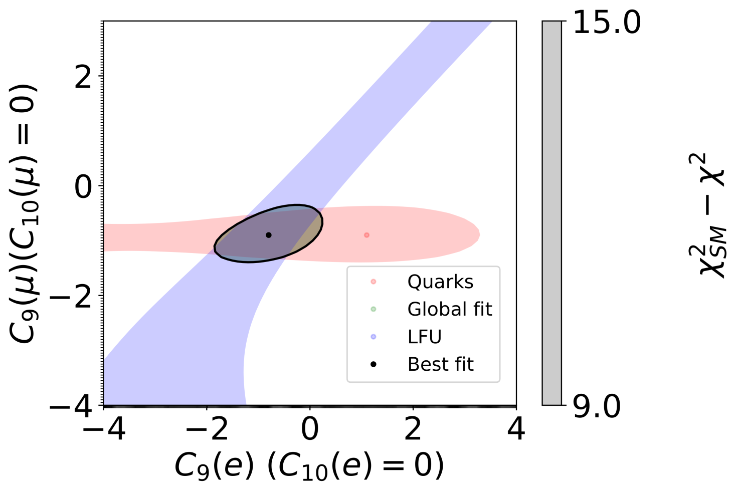
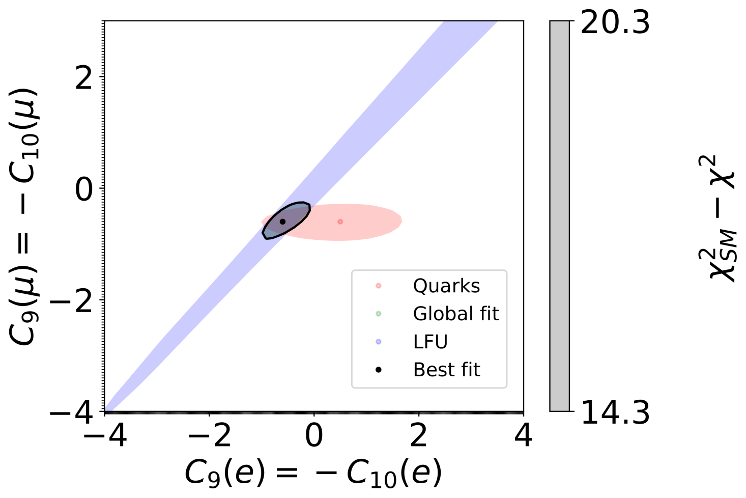
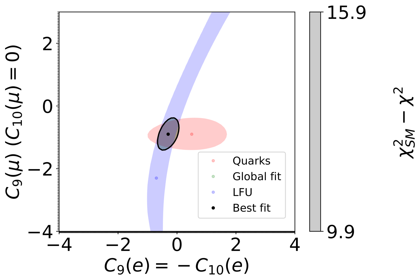
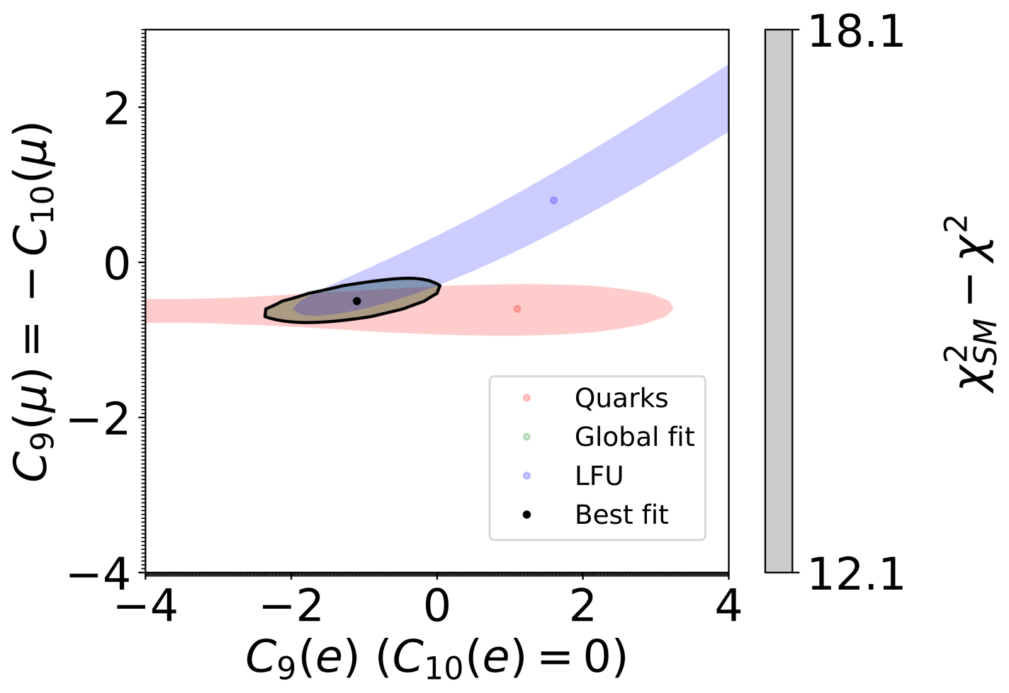
Figure 1: 95$\%$ confidence level (CL) fit regions in the SMEFT parameter space where (top-left) $C_{10}^{(e)}=C_{10}^{(\mu)}=0$, (top-right) $C_{9}^{(\mu)}=-C_{10}^{(\mu)}$ and $C_{9}^{(e)}=-C_{10}^{(e)}$, (bottom-left) $C_{9}^{(e)}=-C_{10}^{(e)}$ and $C_{10}^{(\mu)}=0$, (bottom-right) $C_{10}^{(e)}=0$ and $C_{9}^{(\mu)}=-C_{10}^{(\mu)}$ via (4), (5). ‘LFU’ contains 23 measurements from Belle, LHCb and BaBar which test lepton flavour universality. ‘quarks’ contains the 224 other $b\rightarrow s\mu^{+}\mu^{-}$ measurements defined in flavio2.3.3. The grey colour bar on the right-hand side is labelled with the extremes of the $\chi^{2}_{SM}-\chi^{2}$ values within the 95$\%$ ‘global’ contour. A positive value of $\chi^{2}_{SM}-\chi^{2}$ indicates an improvement of the fit with respect to the SM. The best fit is shown by the black point.

The final scenario we consider is Fig. 1 (bottom-right) where the couplings to new physics are swapped compared with the scenario in the bottom-left panel such that di-muon pairs have left-handed couplings and di-electron pairs have vector-like couplings. A larger range of good-fit values for $C_{9}^{(e)}$ result for this scenario; it is a case with a fit that includes values extending below $C_{9}^{(e)}=-1$.

The main outcome of Ref. Alguero:2023jeh is to evaluate global fits with and without new physics contributions to electron modes under a framework containing updates to both experimental measurements and theoretical calculations of form factors. Within this fully updated framework, the results in that reference identify that new physics introduced by $C_{9}^{(\mu)}$ is mildly preferred over scenarios with $C_{9}^{(\mu)}=-C_{10}^{(\mu)}$, favouring a vector-like coupling to di-muon pairs over a left-handed coupling. The fit also reveals that data can be compatible with non-zero $C_{10}^{(\mu)}$, although support for these scenarios is not as strong.

Other analyses support the introduction of non-zero new physics WCs, though with different assumptions to ours. For example, a recent evaluation including possible new physics WCs Wen:2023pfq performed higher dimensional global fits for several more non-zero WCs instead of focusing on the four that we examine here. There is therefore no overlap between our results and those of Ref. Wen:2023pfq . Another fit assumes that new physics affects electrons and muons identically SinghChundawat:2022zdf , an assumption which we do not follow in the present paper.

Both Refs. Alguero:2023jeh and Wen:2023pfq provide insight into a renewed focus on LFU new physics by examining the differences between global fits before and after the release of the 2022 LHCb update of $R_{K}$ and $R_{K^{\star}}$. The large impact of such observables on constraining the parameter plane $C_{9}^{(e)}-C_{9}^{(\mu)}$ can be seen in Fig. 1.

Fig. 1 indicates that the a best-fit point has $C_{9}^{(e)}\approx C_{9}^{(\mu)}\neq 0$, but that $C_{9}^{(e)}=0$ can also fit the data, as shown in the top-left hand panel. Motivated by this top-left hand panel and similar previous results in Ref. Alguero:2023jeh we shall now turn to a set of models which interpolates between $C_{9}^{(e)}=C_{9}^{(\mu)}\neq 0$ and $C_{9}^{(e)}=0$ (and which also extrapolates outside of these constraints).

3 Models

Our $U(1)_{X}$ gauge symmetry (which is extra to the gauge symmetry of the SM) is expected to be spontaneously broken by a complex scalar ‘flavon’ field $\theta$, whose $U(1)_{X}$ charge $Q$ is non-zero. Of the models we shall propose, aspects such as these just mentioned are very similar to the $U(1)_{Y_{3}-x(L_{\mu}-L_{\tau})}$ model Davighi:2021oel , the $U(1)_{B_{3}-L_{2}}$ model Bonilla:2017lsq ; Alonso:2017uky ; Chun:2018ibr ; Allanach:2020kss , Third Family Hypercharge models (TFHMs) Allanach:2018lvl ; Allanach:2019iiy , or mixtures between the $U(1)_{B_{3}-L_{2}}$ model and the TFHM Allanach:2022bik . The massive electrically neutral gauge boson resulting from Higgsed $U(1)_{X}$ breaking is dubbed a $Z^{\prime}$ boson which has a mass

$$M_{Z^{\prime}}=Qg_{Z^{\prime}}\langle\theta\rangle,$$ (8)

where $\langle\theta\rangle$ is the vacuum expectation value of the flavon field. Whichever fields possess non-zero $U(1)_{X}$ charges will generically have couplings to the $Z^{\prime}$ boson. Thus we wish second-family leptons to have a non-zero charge, and (following the arguments in §1), possibly first-family leptons as well. We also wish the third family of quarks to have a charge in order to establish a $Z^{\prime}$ coupling to $s\bar{b}+H.c.$, starting from a coupling to $b\bar{b}$ in the weak eigenbasis, as also explained in §1. Then, we may explain the $b\rightarrow s\ell^{+}\ell^{-}$ anomalies by new physics contributions to the amplitude like the one depicted in Fig. 2.

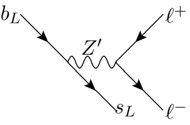
Figure 2: Feynman diagram of the leading new physics contribution to $b\rightarrow s\ell^{+}\ell^{-}$ observables from a suitable $Z^{\prime}$ model.

It should be evident from the above discussion that the charges of the various fields in the model affect the phenomenology of it, since they determine what the $Z^{\prime}$ couples to (and with which relative strength). Therefore, we now discuss the fermionic charge assignment of the model.

3.1 Fermionic charge assignment

We begin by extending the SM by three right-handed neutrino fields $\nu_{i}$. These $\nu_{i}$ fields will be used both for anomaly cancellation, with an eye to ultimately providing an ultra-violet model of neutrino masses (this we shall not specify in any detail, however). The chiral fermionic field content of the model and its representations under the SM$\times U(1)_{X}$ gauge group is specified in Table 1. We note here that for brevity we shall denote both the field and its $U(1)_{X}$ charge by the same label; context should make the meaning of the symbol clear.

Field	$(SU(3),SU(2),U(1)_{Y},U(1)_{X})$
$Q_{i}$	$(3,2,1,Q_{i})$
$L_{i}$	$(1,2,3,L_{i})$
$u_{i}$	$(3,1,4,u_{i})$
$d_{i}$	$(3,1,-2,d_{i})$
$e_{i}$	$(1,1,-6,e_{i})$
$\nu_{i}$	$(1,1,0,\nu_{i})$

Table 1: Representations of fermionic chiral fields under the SM$\times U(1)_{X}$ gauge group. $i\in\{1,2,3\}$ is a family index and gauge indices have been suppressed. $Q_{i}$ and $L_{i}$ are left-handed Weyl fermions, whereas the other fields listed are all right-handed Weyl fermions. We have chosen here to normalise the hypercharge gauge coupling so that the hypercharges of all fermionic fields are integers.

As explained above, we want to find a set of models that can potentially address the $b\rightarrow s\mu^{+}\mu^{-}$ anomalies, but which interpolate between models where the $Z^{\prime}$ does not couple to electrons and those where it couples with an equal strength to di-electron pairs and di-muon pairs. However, the $U(1)_{X}$ charge assignments have constraints upon them given by the requirement of not generating quantum field theoretic anomalies, which would spoil the gauge symmetry. We shall now go through the arguments that lead us to the charge assignments, since they shall make clear to which extent the assignments are constrained by anomaly cancellation, to which extent they are a choice dictated by desired phenomenology and the extent to which they are just a choice to be concrete.

We first list the anomaly cancellation conditions which a gauged $U(1)_{X}$ chiral-fermion charge assignment should respect Allanach:2018vjg :

$$\sum_{i}\left(2Q_{i}-u_{i}-d_{i}\right) = 0,$$ (9)

$$\sum_{i}\left(L_{i}+3Q_{i}\right) = 0,$$ (10)

$$\sum_{i}\left(Q_{i}+3L_{i}-8u_{i}-2d_{i}-6e_{i}\right) = 0,$$ (11)

$$\sum_{i}\left(6Q_{i}+2L_{i}-3u_{i}-3d_{i}-e_{i}-\nu_{i}\right) = 0,$$ (12)

$$\sum_{i}\left(Q_{i}^{2}-L_{i}^{2}-2u_{i}^{2}+d_{i}^{2}+e_{i}^{2}\right) = 0$$ (13)

$$\sum_{i}\left(6Q_{i}^{3}+2L_{i}^{3}-3u_{i}^{3}-3d_{i}^{3}-e_{i}^{3}-\nu_{i}^{3}\right) = 0.$$ (14)

These equations have been simultaneously solved over the integers both numerically with $U(1)_{X}$ charges between 10 and -10 Allanach:2018vjg and, more generally, analytically Allanach:2020zna . Rather than begin with these solutions and then restrict them, we instead find it instructive to make some choices based partly on expected phenomenological consequences of some charge assignments whilst simultaneously applying (9)-(14).

We require a coupling of the $Z^{\prime}$ to left-handed $b\bar{s}$ quark pairs in order to explain an apparent new physics effect in $b\rightarrow s\mu^{+}\mu^{-}$ transitions. We therefore pick $Q_{3}\neq 0$, providing a $Z^{\prime}$ coupling to left-handed $b\bar{b}$ pairs and assume that its coupling to (left-handed) $\bar{b}s+H.c.$ will be provided by some small amount of $b-s$ mixing. The mixing is banned by $U(1)_{X}$ but since this is spontaneously broken, we anticipate small $U(1)_{X}$ breaking effects, such as small quark mixing. We may fix $Q_{3}=1$ by rescaling the $U(1)_{X}$ gauge coupling. If we couple the $Z^{\prime}$ dominantly to the third family quarks only, direct $Z^{\prime}$ search bounds from the LHC will be weaker, since LHC $Z^{\prime}$ production dominantly occurs via the $b\bar{b}\rightarrow Z^{\prime}$ process, which is doubly suppressed by both the $b$ and $\bar{b}$ parton distribution functions. Motivated by this, we fix the $U(1)_{X}$ charges of the first two generations of quark fields to zero, i.e. $u_{1}=u_{2}=d_{1}=d_{2}=Q_{1}=Q_{2}=0$. Substituting these assignments into (9), we obtain that $u_{3}+d_{3}=2$. We shall here pick $u_{3}=d_{3}=1$, meaning that we can characterise the quark charges in terms of third-family baryon number. (10) then gives that

$$\sum_{i}L_{i}=-3.$$ (15)

We shall pick $L_{2}\neq 0$ in order to couple the $Z^{\prime}$ to left-handed muon pairs, since we know from fits to $b\rightarrow s\mu^{+}\mu^{-}$ anomalies Alguero:2023jeh ; Wen:2023pfq that a new physics contribution to $C_{9}^{(\mu)}\neq 0$ is necessary to describe the pertinent measurements well. We shall vary $L_{1}$ in order to vary the $Z^{\prime}$ coupling to left-handed electron pairs: (15) then can be rearranged to yield $L_{3}$. Substituting (15) and the other assigned charges into (11), we obtain

$$\sum_{i}e_{i}=-3,$$ (16)

which allows us to obtain, using (12),

$$\sum_{i}\nu_{i}=-3.$$ (17)

(13) and (14) then become

$$\sum_{i}\left(L_{i}^{2}-e_{i}^{2}\right)=0,$$ (18)

$$\sum_{i}\left(2L_{i}^{3}-e_{i}^{3}-\nu_{i}^{3}\right)=0.$$ (19)

(16)-(19) are solved by

$$L_{i}=e_{i}=\nu_{i}\ \text{for each}\ i.$$ (20)

This is not a general solution of the equations, but it is sufficient for our purposes here. After the stipulation in (20), there remains only one independent constraint, which we can take to be (15). (20) allows us to summarise the $U(1)_{X}$ charges in terms of electron number $L_{e}$, muon number $L_{\mu}$ and tau number $L_{\tau}$. We shall fix the $X$ charge of $L_{2}=e_{2}=\nu_{2}$ (here dubbed to be $-X_{\mu}$) to be a reasonably large integer to allow more resolution in the other charges; we pick $X_{\mu}=10$. We then allow the $U(1)_{X}$ electron charge ($-X_{e}$) to vary. The $U(1)_{X}$ charges of the fermions as a whole can be characterised by

$$3B_{3}-\left(X_{e}L_{e}+X_{\mu}L_{\mu}+[3-X_{e}-X_{\mu}]L_{\tau}\right).$$ (21)

$X_{e}/X_{\mu}=1$ corresponds to the case where the coupling of the $Z^{\prime}$ to di-electron pairs is equal to that of di-muon pairs, whereas $X_{e}=0$ is the case where the electron does not directly couple to the $Z^{\prime}$ at tree-level.

The arguments on anomaly cancellation thus far apply to our assumed chiral fermionic content of the SM plus three right-handed neutrinos. If one were add a pair of chiral fermions which are vector-like under the SM gauge symmetries but have non-cancelling $U(1)_{X}$ charges, the system of anomaly equations would change and one could acquire different solutions to the ones that we have found. One would need to explain how these additional chiral fermions acquire masses to make them significantly heavier than is probed by current experiments; this might be possible, depending upon the new chiral fermion charges, by utilising $U(1)_{X}$ breaking effects via $\langle\theta\rangle\approx{\mathcal{O}}$(TeV). We note this caveat, but shall for now assume no additional chiral fermionic fields of this type. Our anomaly cancellation analysis applies to the chiral fermionic field content in Table 1 along with any additional fermions only being added in vector-like pairs under the entire SM$\times U(1)_{X}$ gauge group.

We fix the $U(1)_{X}$ charge of the SM Higgs doublet $H$ so that the top Yukawa coupling Lagrangian density term, $\lambda_{t}\overline{Q_{3}}Hu_{3}+H.c.$, is allowed by the gauge symmetry. This constraint requires that $H$ then has $U(1)_{X}$ charge equal to zero, simplifying our analysis because there is no predicted $Z-Z^{\prime}$ mixing at tree-level. Such a mixing would change the predictions of electroweak precision observables (EWPOs); with zero mixing, as predicted here, we effectively decouple the EWPOs from our discussion. This is essentially dictated by model choice: in other models, e.g. the TFHMs, the electroweak observables significantly change with model parameters (the quality of the electroweak fit in the TFHMs is similar to that of the SM, with improvements in $M_{W}$ being offset against other EWPOs such as measurements of $Z^{0}$ boson couplings to different families of di-lepton pair Allanach:2021kzj ). Thus, decoupling the EWPOs as we do here simplifies our analysis but is not necessarily essential phenomenologically: the preference (or otherwise) of electroweak fits has to be determined on a case-by-case basis.

It behoves us now to specify the other pertinent TeV-scale properties of our model, which we shall do in the following subsection.

3.2 More model details

Here, we deal with the $Z^{\prime}$-specific parts of the model, which encapsulates the phenomenology that we are interested in predicting. We shall not find it necessary to specify all details of the model (the flavon potential or flavon/Higgs mixing – for that, see Ref. Allanach:2022blr – or the origin of non-zero small Yukawa couplings, for example). The model set-up in the present subsection closely follows that of Refs. Allanach:2018lvl ; Allanach:2019iiy ; Allanach:2020kss ; Allanach:2022bik , which are discriminated from the present model by the fermionic $U(1)_{X}$ charge assignments. The model is supposed to be at the level of a TeV-scale effective field theory that includes the quantum fields of the SM, three right-handed neutrino fields and the $Z^{\prime}$. We write the fermionic fields in the gauge eigenbasis with a primed notation

$${\bf u_{L}^{\prime}} = \left(\begin{array}[]{c}u_{L}^{\prime}\\ c_{L}^{\prime}\\ t_{L}^{\prime}\\ \end{array}\right),\qquad{\bf d_{L}^{\prime}}=\left(\begin{array}[]{c}d_{L}^{\prime}\\ s_{L}^{\prime}\\ b_{L}^{\prime}\\ \end{array}\right),\qquad{\bf e_{L}^{\prime}}=\left(\begin{array}[]{c}e_{L}^{\prime}\\ \mu_{L}^{\prime}\\ \tau_{L}^{\prime}\\ \end{array}\right),\qquad{\bm{\nu}_{L}^{\prime}}=\left(\begin{array}[]{c}{\nu_{e}^{\prime}}_{L}\\ {\nu_{\mu}^{\prime}}_{L}\\ {\nu_{\tau}^{\prime}}_{L}\\ \end{array}\right),$$ (34)

$${\bf u_{R}^{\prime}} = \left(\begin{array}[]{c}u_{R}^{\prime}\\ c_{R}^{\prime}\\ t_{R}^{\prime}\\ \end{array}\right),\qquad{\bf d_{R}^{\prime}}=\left(\begin{array}[]{c}d_{R}^{\prime}\\ s_{R}^{\prime}\\ b_{R}^{\prime}\\ \end{array}\right),\qquad{\bf e_{R}^{\prime}}=\left(\begin{array}[]{c}e_{R}^{\prime}\\ \mu_{R}^{\prime}\\ \tau_{R}^{\prime}\\ \end{array}\right),\qquad{\bm{\nu}_{R}^{\prime}}=\left(\begin{array}[]{c}{\nu_{e}^{\prime}}_{R}\\ {\nu_{\mu}^{\prime}}_{R}\\ {\nu_{\tau}^{\prime}}_{R}\\ \end{array}\right),$$ (47)

along with the SM fermionic electroweak doublets

$${\bf Q^{\prime}}_{i}=\left(\begin{array}[]{c}{\bf u_{L}^{\prime}}_{i}\\ {\bf d_{L}^{\prime}}_{i}\end{array}\right),\qquad{\bf L^{\prime}}_{i}=\left(\begin{array}[]{c}{\bm{\nu}_{L}^{\prime}}_{i}\\ {\bf e_{L}^{\prime}}_{i}\end{array}\right).$$ (48)

The neutrinos and SM fermions acquire masses after the SM Brout-Englert-Higgs mechanism through

$$-\mathcal{L}_{Y} = \overline{\bf Q^{\prime}}Y_{u}\tilde{H}{\bf u^{\prime}_{R}}+\overline{\bf Q^{\prime}}Y_{d}H{\bf d^{\prime}_{R}}+\overline{\bf L^{\prime}}Y_{e}H{\bf e^{\prime}_{R}}+\overline{\bf L}Y_{\nu}\tilde{H}{\bm{\nu}^{\prime}_{R}}+\frac{1}{2}{\overline{{\bm{\nu}_{R}^{\prime}}^{c}}}M{\bm{\nu}_{R}^{\prime}}+H.c.,$$ (49)

where $Y_{u}$, $Y_{d}$ and $Y_{e}$ are dimensionless complex coupling constants, each written as a 3 by 3 matrix in family space; the matrix $M$ is a 3 by 3 complex symmetric matrix of mass dimension 1, ${\Phi}^{c}$ denotes the charge conjugate of field $\Phi$ and $\tilde{H}:=({H^{0}}^{\ast},-H^{-})^{T}$. Gauge indices have been omitted in (49).

For $X_{e}\neq X_{\mu}\neq X_{\tau}$, the Yukawa couplings have the following textures at the renormalisable tree level in the unbroken $U(1)_{X}$ limit:

$$Y_{u}\sim\begin{pmatrix}\times&\times&0\\ \times&\times&0\\ 0&0&\times\\ \end{pmatrix},\quad Y_{d}\sim\begin{pmatrix}\times&\times&0\\ \times&\times&0\\ 0&0&\times\\ \end{pmatrix},\quad Y_{e}\sim\begin{pmatrix}\times&0&0\\ 0&\times&0\\ 0&0&\times\\ \end{pmatrix}.$$ (50)

The structure of $Y_{e}$ predicts that charged-lepton violating couplings of the $Z^{\prime}$ are zero.

We may write $H=(0,\ (v+h)/\sqrt{2})^{T}$ after electroweak symmetry breaking, where $h$ is the physical Higgs boson field and (49) includes the fermion mass terms

$$-\mathcal{L}_{Y} = \overline{\bf u^{\prime}_{L}}V_{u_{L}}V_{u_{L}}^{\dagger}m_{u}V_{u_{R}}V_{u_{R}}^{\dagger}{\bf u^{\prime}_{R}}+\overline{\bf d^{\prime}_{L}}V_{d_{L}}V_{d_{L}}^{\dagger}m_{d}V_{d_{R}}V_{d_{R}}^{\dagger}{\bf d^{\prime}_{R}}+\overline{\bf e^{\prime}_{L}}V_{e_{L}}V_{e_{L}}^{\dagger}m_{e}V_{e_{R}}V_{e_{R}}^{\dagger}{\bf e^{\prime}_{R}}+$$ (53)

$$\frac{1}{2}({\overline{\bm{\nu}_{L}^{\prime}}}\ \overline{{\bm{\nu}_{R}^{\prime}}^{c}})M_{\nu}\left(\begin{array}[]{c}{\bm{\nu_{L}^{\prime}}}^{c}\\ {\bm{\nu}_{R}^{\prime}}\\ \end{array}\right)+H.c.+\ldots,$$

where

$$M_{\nu}=\left(\begin{array}[]{cc}0&m_{\nu_{D}}\\ m_{\nu_{D}}^{T}&M\\ \end{array}\right),$$ (54)

$V_{I_{L}}$ and $V_{I_{R}}$ are 3 by 3 unitary mixing matrices for each field species $I$, $m_{u}:=vY_{u}/\sqrt{2}$, $m_{d}:=vY_{d}/\sqrt{2}$, $m_{e}:=vY_{e}/\sqrt{2}$ and $m_{\nu_{D}}:=vY_{\nu}/\sqrt{2}$, where $v$ is the SM Higgs expectation value, measured to be 246.22 GeV ParticleDataGroup:2022pth . The final explicit term in (53) incorporates the see-saw mechanism via a 6 by 6 complex symmetric mass matrix. Since the elements in $m_{\nu_{D}}$ are much smaller than those in $M$, we perform a rotation to obtain a 3 by 3 complex symmetric mass matrix for the three light neutrinos. These approximately coincide with the left-handed weak eigenstates ${\bm{\nu}^{\prime}_{L}}$, whereas three heavy neutrinos approximately correspond to the right-handed weak eigenstates ${\bm{\nu}^{\prime}_{R}}$. The neutrino mass term of (53) becomes, to a good approximation,

$$-{\mathcal{L}}_{\nu}=\frac{1}{2}{\overline{\bm{\nu}_{L}^{\prime c}}}m_{\nu}{\bm{\nu}_{L}^{\prime}}+\frac{1}{2}{\overline{\bm{\nu}_{R}^{\prime c}}}M{\bm{\nu}_{R}^{\prime}}+H.c.,$$ (55)

where $m_{\nu}:=m_{\nu_{D}}^{T}M^{-1}m_{\nu_{D}}$ is a complex symmetric 3 by 3 matrix.

Choosing $V_{I_{L}}^{\dagger}m_{I}V_{I_{R}}$ to be diagonal, real and positive for $I\in\{u,d,e\}$, and $V_{{\nu}_{L}}^{T}m_{\nu}V_{{\nu}_{L}}$ to be diagonal, real and positive (all in ascending order of mass from the top left toward the bottom right of the matrix), we can identify the non-primed mass eigenstates

$${{\bf P}}=V_{P}^{\dagger}{\bf P^{\prime}}\ \text{where}\ {P}\in\{{u_{R}},\ {d_{L}},\ {u_{L}},\ {e_{R}},\ {u_{R}},\ {d_{R}},\ {\nu}_{L},\ {e_{L}}\}.$$ (56)

We may then find the CKM matrix $V$ and the Pontecorvo-Maki-Nakagawa-Sakata (PMNS) matrix $U$ in terms of the fermionic mixing matrices:

$$V=V_{u_{L}}^{\dagger}V_{d_{L}},\qquad U=V_{\nu_{L}}^{\dagger}V_{e_{L}}.$$ (57)

The zeroes in $Y_{u}$ and $Y_{d}$ in (50) predict that the magnitudes of the elements $V_{23},V_{13},V_{32},V_{31}$ are much smaller than 1, agreeing with measurements ParticleDataGroup:2022pth . Clearly, more model building into the ultra-violet would be required to understand the details of neutrino masses and mixing and how exactly the zeroes in (50) are filled in with small entries. We leave such model considerations aside, instead pointing to §2.5 of Ref. Allanach:2022iod for some possibilities.

The kinetic terms of the $U(1)_{X}$ gauge boson yield the following $Z^{\prime}$ interactions

$${\mathcal{L}}_{I}=-g_{Z^{\prime}}\left(\overline{\bf Q^{\prime}}\not{Z}^{\prime}\xi{\bf Q^{\prime}}+\overline{\bf u^{\prime}_{R}}\not{Z}^{\prime}\xi{\bf u^{\prime}_{R}}+\overline{d^{\prime}_{R}}\not{Z}^{\prime}\xi{\bf d^{\prime}_{R}}+\overline{\bf L^{\prime}}\not{Z}^{\prime}\Xi{\bf L^{\prime}}+\overline{\bf e^{\prime}_{R}}\not{Z}^{\prime}\Xi{\bf e^{\prime}_{R}}+\overline{{\bm{\nu}^{\prime}_{R}}}\not{Z}^{\prime}\Xi{{\bm{\nu}^{\prime}_{R}}}\right),$$ (58)

where

$$\xi:=\begin{pmatrix}0&0&0\\ 0&0&0\\ 0&0&1\\ \end{pmatrix},\qquad\Xi:=\begin{pmatrix}-X_{e}&0&0\\ 0&-X_{\mu}&0\\ 0&0&-X_{\tau}\\ \end{pmatrix}$$ (59)

are fixed by the fermionic fields’ $U(1)_{X}$ charges. The right-handed neutrinos ${\bm{\nu}^{\prime}_{R}}$ are assumed to be heavy compared to the TeV scale and play no further role in the phenomenology of $b\rightarrow s\mu^{+}\mu^{-}$ anomalies; we shall therefore neglect them in the discussion that follows. In the unprimed mass eigenbasis, (58) becomes

$${\mathcal{L}}_{I} = -g_{Z^{\prime}}\left(\overline{\bf u_{L}}\not{Z}^{\prime}\Lambda_{\xi}^{u_{L}}{\bf u_{L}}+\overline{\bf d_{L}}\not{Z}^{\prime}\Lambda_{\xi}^{d_{L}}{\bf d_{L}}+\overline{\bf u_{R}}\not{Z}^{\prime}\Lambda_{\xi}^{u_{R}}{\bf u_{R}}+\overline{\bf d_{R}}\not{Z}^{\prime}\Lambda_{\xi}^{d_{R}}{\bf d_{R}}+\right.$$ (60)

$$\left.\overline{\bf e_{L}}\not{Z}^{\prime}\Lambda_{\Xi}^{e_{L}}{\bf e_{L}}+\overline{\bf e_{R}}\not{Z}^{\prime}\Lambda_{\Xi}^{e_{R}}{\bf e_{R}}+\overline{\bm{\nu}_{L}}\not{Z}^{\prime}\Lambda_{\Xi}^{\nu_{L}}{\bm{\nu}_{L}}+\overline{\bm{\nu}_{R}}\not{Z}^{\prime}\Lambda_{\Xi}^{\nu_{R}}{\bm{\nu}_{R}}\right),$$

where $\Lambda_{\alpha}^{P}:=V_{P}\alpha V_{P}^{\dagger}$ for $P\neq\nu_{L}$ and $\alpha\in\{\xi,\Xi\}$. $\Lambda_{\alpha}^{\nu}:=V_{P}\alpha V_{P}^{T}$

To make phenomenological progress with our models, we shall need to specify $V_{P}$. We simply assume that the ultra-violet model details are such that the zeroes in (50) are filled in (or not) at the correct level for experiment. The $V_{P}$ are 3 by 3 unitary matrices, and we pick a simple ansatz which is not immediately obviously ruled out by strong flavour changing neutral current constraints on charged lepton flavour violation or neutral current flavour violation in the first two families of quark. Firstly, we set $V_{e_{R}}=V_{d_{R}}=V_{u_{R}}=V_{e_{L}}=I$, the 3 by 3 identity matrix. A non-zero $(V_{d_{L}})_{23}$ matrix element is required for the $Z^{\prime}$ to mediate new physics contributions to $b\rightarrow s\ell^{+}\ell^{-}$ transitions. We capture the important quark mixing (i.e. between $s_{L}$ and $b_{L}$) in $V_{d_{L}}$ as

$$V_{d_{L}}=\left(\begin{array}[]{ccc}1&0&0\\ 0&\cos\theta_{sb}&\sin\theta_{sb}\\ 0&-\sin\theta_{sb}&\cos\theta_{sb}\\ \end{array}\right).$$ (61)

$V_{\nu_{L}}$ and $V_{u_{L}}$ are fixed by (57), where we use the experimentally determined values for the entries of $V$ and $U$ via the central values in the standard parameterisation from Ref. ParticleDataGroup:2022pth . Having fixed all of the fermionic mixing matrices, we have provided an ansatz that could be perturbed around for a more complete characterisation. We leave such perturbations aside in the present paper.

Here, we summarise the SMEFT operators that result from integrating out the $Z^{\prime}$; they are given in Table 2, ready for input into flavio2.3.3 Straub:2018kue .

WC	value	WC	value
$C_{ll}^{iiii}$	$-\frac{1}{2}L_{i}^{2}$	$C_{ll}^{iijj}$ $(i\neq j)$	$-L_{i}L_{j}$
$(C_{lq}^{(1)})^{iijk}$	$L_{i}(\Lambda_{\Xi}^{(d_{L})})_{jk}$
$C_{ee}^{iijj}$ $(i\neq j)$	$-L_{i}L_{j}$	$C_{uu}^{3333}$	$-\frac{1}{2}$
$C_{dd}^{3333}$	$-\frac{1}{2}$	$C_{ee}^{iiii}$	$-\frac{1}{2}L_{i}^{2}$
$C_{eu}^{ii33}$	$L_{i}$	$C_{ed}^{ii33}$	$L_{i}$
${C_{ud}^{(1)}}^{3333}$	$-1$	$C_{le}^{iijj}$	$-L_{i}L_{j}$
$C_{qe}^{ijkk}$	$L_{k}(\Lambda_{\Xi})_{ij}$	${C_{qu}^{(1)}}^{ij33}$	$-(\Lambda_{\Xi})_{ij}$
${C_{qd}^{(1)}}^{ij33}$	$-(\Lambda_{\Xi})_{ij}$	${C_{qq}^{(1)}}^{ijkl}$	$(\Lambda_{\Xi})_{ij}(\Lambda_{\Xi})_{kl}\frac{\delta_{ik}\delta_{jl}-2}{2}$
$C_{lu}^{ii33}$	$L_{i}$	$C_{ld}^{ii33}$	$L_{i}$

Table 2: Non-zero $M_{Z^{\prime}}$-scale SMEFT operators in units of $g_{Z^{\prime}}^{2}/M_{Z^{\prime}}^{2}$, in terms of the left-handed lepton doublet $U(1)_{X}$ charges $L_{i}$. The notation is in the down-aligned Warsaw basis Grzadkowski:2010es . There is no sum implied upon repeated family indices $i,j,k,l\in\{1,2,3\}$.

We note that, to specify the model and its $Z^{\prime}$ phenomenology, once we have picked a value for $X_{e}$, there are three important model parameters that affect the pertinent phenomenology: $g_{Z^{\prime}}$, $M_{Z^{\prime}}$ and $\theta_{sb}$, but at tree-level, as Table 2 shows, the flavour data only depend upon two effective parameters: the combination $g_{Z^{\prime}}/M_{Z^{\prime}}$ and $\theta_{sb}$.

4 LEP constraints

Since some of the models we consider couple the $Z^{\prime}$ to di-electron pairs, LEP-2 di-lepton production cross-section measurements, which are broadly in agreement with SM predictions, provide constraints. This is because a contribution from the $Z^{\prime}$ becomes non-zero: some leading Feynman diagrams for its contribution to the amplitude are shown in Fig. 3.

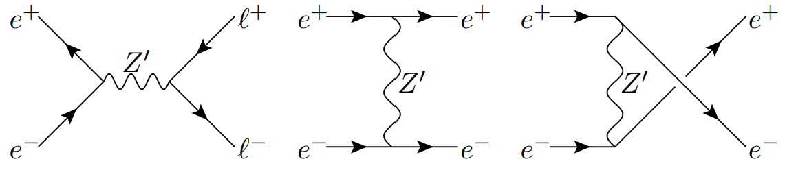
Figure 3: Feynman diagram of the leading $Z^{\prime}$ contribution to LEP-2 di-lepton production from a suitable model. Here, $\ell\in\{e,\mu,\tau\}$.

In this section, we shall re-examine the constraints on four-lepton dimension-6 SMEFT WCs coming from LEP-2. Analytic expressions for the expected dominant contributions from these (in the interference terms) have been already calculated in Ref. Falkowski:2015krw . Here, we re-calculate the full dependence of the tree-level predictions upon the WCs ready for inclusion into flavio2.3.3. By extracting the interference terms, we shall provide an independent check upon the analytic results presented in Ref. Falkowski:2015krw . By calculating the full tree-level dependence upon the WCs (i.e. not only including the interference terms) and putting them into flavio2.3.3, we evade possible computational problems with predicted negative cross-sections when performing parameter scans. Ref. Falkowski:2015krw provided numerical results of a fit to electroweak measurements of the epoch and other LEP measurements, where some of the WCs are constrained at the $\mathcal{O}(10^{-2})/v^{2}$ level, where $v=246.22$ GeV is the SM Higgs vacuum expectation value. Although LEP experimental measurements have not changed since Ref. Falkowski:2015krw , some electroweak data have. Providing the LEP constraints as part of the flavio2.3.3 package should then facilitate SMEFT fits in general as well as fits to our $Z^{\prime}$ models, once we have matched the models to the SMEFT.

Some of the SMEFT WCs alter differential scattering cross-section predictions of $e^{+}e^{-}\rightarrow\mu^{+}\mu^{-}$, $e^{+}e^{-}\rightarrow\tau^{+}\tau^{-}$ and $e^{+}e^{-}\rightarrow e^{+}e^{-}$ (Bhabha scattering). In the Warsaw convention Grzadkowski:2010es , the relevant WCs which can alter the predictions for these processes are $C_{le}^{1jj1}$, $C_{ll}^{11jj}$, $C_{ee}^{11jj}$, $C_{le}^{11jj}$ and $C_{le}^{11jj}$, where $j\in\{1,2,3\}$. The predictions for $e^{+}e^{-}\rightarrow\mu^{+}\mu^{-}$ and $e^{+}e^{-}\rightarrow\tau^{+}\tau^{-}$ are simple and almost identical to each other and so we consider them first, before going on to consider Bhabha scattering.

4.1 LEP: di-muon and di-tau final states

Building notation similar to that in Ref. Greljo:2022jac , we consider the tree-level polarised scattering amplitudes of massless di-electron pairs into either massless di-muon pairs ($j=2$) or massless di-tau pairs ($j=3$) including 4-lepton dimension-6 SMEFT operators

$${\mathcal{M}}\left(e^{+}e^{-}\rightarrow e_{j}^{+}e_{j}^{-}\right)=-i\left(\bar{e}\gamma^{\alpha}P_{L}e_{j}\right)\left(\bar{e}_{j}\gamma_{\alpha}P_{R}e\right)C_{le}^{1jj1}+i\sum_{X,Y}\left(\bar{e}\gamma^{\alpha}P_{X}e\right)\left(\bar{e}_{j}\gamma_{\alpha}P_{Y}e_{j}\right)N_{1jj1}^{XY}(s),$$ (62)

where the sum is over $\{X,Y\}\in\{L,R\}$,

$$N_{1jj1}^{XY}(s) := \frac{e^{2}}{s}+\frac{g_{Z}^{e_{X}}g_{Z}^{{e_{j}}_{Y}}}{s-M_{Z}^{2}+i\Gamma_{Z}M_{Z}}+\left(C_{ll}^{11jj}+C_{ll}^{1jj1}\right)\delta_{XL}\delta_{YL}+C_{ee}^{11jj}\delta_{XR}\delta_{YR}+$$ (63)

$$C_{le}^{11jj}\delta_{XL}\delta_{YR}+C_{le}^{jj11}\delta_{XR}\delta_{YL},$$

$\delta_{LL}=\delta_{RR}=1,\ \delta_{LR}=\delta_{RL}=0$, $s,t$ and $u$ are the usual Mandlestam kinematic variables, $M_{Z}$ is the $Z^{0}$ boson pole mass and the SMEFT WCs $C_{ee}^{ijkm}$, $C_{le}^{ijkm}$ and $C_{ll}^{ijkm}$ (where $i,j,k,m\in\{1,2,3\}$ are family indices) are written in the Warsaw convention Grzadkowski:2010es . $g_{Z}^{e_{X}}$ is the di-$X$-handed electron coupling to the $Z^{0}$ boson including tree-level corrections from SMEFT and $g_{Z}^{e_{j_{Y}}}$ is the di-$Y$-handed $j^{th}$-family coupling to the $Z^{0}$ boson Brivio:2017vri . $\Gamma_{Z}$ is the $Z^{0}$ boson’s total width. Summing over the final spins and averaging over initial spins, we obtain a differential cross-section

$$\frac{d\sigma}{dt}=\frac{1}{16\pi}\left\{|C_{le}^{1jj1}|^{2}+\sum_{X,Y}|N^{XY}_{1jj1}(s)|^{2}\left[\delta_{XY}\left(1+\frac{t}{s}\right)^{2}+(1-\delta_{XY})\frac{t^{2}}{s^{2}}\right]\right\}.$$ (64)

Integrating, we obtain the total cross-section

$$\sigma(e^{+}e^{-}\rightarrow e_{j}^{+}e_{j}^{-})=\frac{s}{48\pi}\left\{3|C_{le}^{1jj1}|^{2}+\sum_{X,Y}|N^{XY}_{1jj1}(s)|^{2}\right\}$$ (65)

and a forward cross-section minus backward cross-section

$$\sigma(e^{+}e^{-}\rightarrow e_{j}^{+}e_{j}^{-})_{F}-\sigma(e^{+}e^{-}\rightarrow e_{j}^{+}e_{j}^{-})_{B}=\frac{s}{64\pi}\sum_{X,Y}\left|N^{XY}_{1jj1}(s)\right|^{2}(2\delta_{XY}-1).$$ (66)

The dimension-6 WC-SM interference terms in (65) and (66) agree with the interference terms derived in Ref. Falkowski:2015krw (in the parameter space considered in Ref. Falkowski:2015krw , such interference terms encapsulate the dominant effects of the SMEFT operators and were the only ones presented explicitly there). (64) shows that the part proportional to $|C_{le}^{1jj1}|^{2}$ does not interfere with the rest of the matrix element due to its different helicity-flavour structure (as already noted in Ref. Falkowski:2015krw ).

In Ref. ALEPH:2013dgf , the SM prediction for the cross-section is given including some higher-order one-loop contributions. By using the ratio of the predicted cross-section to the SM prediction in the constraints, we can effectively include the dominant effects of these higher order contributions. Our implementation in flavio2.3.3 therefore uses such a ratio. Both the ratios of the total cross-section and the forward cross-section minus the backward cross-section are used for the following LEP 2 centre-of-mass energies:

$$E/\text{GeV}\in\{130.3,136.3,161.3,172.1,182.7,188.6,191.6,195.5,199.5,201.8,204.8,206.5\}.$$ (67)

Correlations between the various measurements are neglected for $e^{+}e^{-}\rightarrow\ell^{+}\ell^{-}$, where $\ell\in\{\mu,\tau\}$.

4.2 LEP: Bhabha scattering

We calculate the tree-level polarised amplitude ${\mathcal{M}}$ for $e^{+}(p_{2})e^{-}(p_{1})\rightarrow e^{+}(q_{2})e^{-}(q_{1})$ in the massless electron approximation.

$$-i{\mathcal{M}} = -I_{t}\frac{e^{2}}{t}\ +I_{s}\frac{e^{2}}{s}+\sum_{X,Y}\left\{-\left(\bar{u}\gamma^{\mu}P_{X}u\right)\left(\bar{v}\gamma_{\mu}P_{Y}v\right)t_{XY}+\left(\bar{u}\gamma^{\mu}P_{X}v\right)\left(\bar{v}\gamma_{\mu}P_{Y}u\right)s_{XY}\right\},$$ (68)

where $u:=u(p_{1})$, $v:=v(q_{2})$, $\bar{u}:=\bar{u}(q_{1})$ and $\bar{v}:=\bar{v}(p_{2})$ are the usual positive and negative energy 4-component Dirac spinors of the electron field and

$$I_{t} := \left(\bar{u}\gamma^{\mu}u\right)\left(\bar{v}\gamma_{\mu}v\right),$$

$$I_{s} := \left(\bar{u}\gamma^{\mu}v\right)\left(\bar{v}\gamma_{\mu}u\right),$$

$$t_{XY} := \frac{g_{e_{X}}g_{e_{Y}}}{t-M_{Z}^{2}+i\Gamma_{Z}M_{Z}}+\frac{C_{XY}+C_{YX}}{2},$$

$$s_{XY} := \frac{g_{e_{X}}g_{e_{Y}}}{s-M_{Z}^{2}+i\Gamma_{Z}M_{Z}}+\frac{C_{XY}+C_{YX}}{2}$$ (69)

and $C_{LL}:={C_{ll}^{(1)}}^{1111}$, $C_{RR}:=C_{ee}^{1111}$, $C_{LR}:=C_{le}^{1111}$ and $C_{RL}:=C_{le}^{1111}$. The spin summed/averaged differential cross-section in the centre-of-mass frame is then

$$\frac{d\sigma}{d\cos\theta} = \frac{1}{32\pi s}\left(2e^{4}\left[\frac{u^{2}+t^{2}}{t^{2}}+\frac{u^{2}+t^{2}}{s^{2}}+\frac{2u^{2}}{st}\right]+\right.$$

$$\sum_{X,Y}\left\{\frac{2e^{2}}{t}\left(\text{Re}(t_{XY})\left[u^{2}\delta_{XY}+s^{2}(1-\delta_{XY})\right]+\text{Re}(s_{XY})u^{2}\delta_{XY}\right)+\right.$$

$$\frac{2e^{2}}{s}\left(\text{Re}(s_{XY})\left[u^{2}\delta_{XY}+t^{2}(1-\delta_{XY})\right]+\text{Re}(t_{XY})u^{2}\delta_{XY}\right)+$$

$$\left.\left.|t_{XY}|^{2}[u^{2}\delta_{XY}+s^{2}(1-\delta_{XY})]+|s_{XY}|^{2}[u^{2}\delta_{XY}+t^{2}(1-\delta_{XY})]+\right.\right.$$

$$\left.\left.2\text{Re}(t_{XY}^{\dagger}s_{XY})u^{2}\delta_{XY}\right\}\right),$$

where $\theta$ is the scattering angle. Extracting the dimension-6 SMEFT WC-SM interference terms from (4.2), we observe agreement with Ref. Falkowski:2015krw , providing an independent check on both calculations. In order to implement the Bhabha scattering constraints into flavio2.3.3 we have integrated (4.2) with respect to $\cos\theta$ (utilising $t=-s(1-\cos\theta)/2$ and $u=-s(1+\cos\theta)/2$), since the combined LEP2 data in Ref. ALEPH:2013dgf are given in bins of $\cos\theta$. The resulting expression is rather large, so we do not list it here, although we note that it can be found in the ancillary information stored with the arXiv version of this paper.

Ref. ALEPH:2013dgf combined LEP-experiment cross-sections for $e^{+}e^{-}\rightarrow e^{+}e^{-}$ for centre-of-mass energies between 189 GeV and 207 GeV and in bins of $\cos\theta$ in the interval $[-0.9,0.9]$ were presented. The SM prediction of the binned cross-sections were also given and we shall again constrain the ratio of the measured cross-section to the SM prediction in order to constrain SMEFT operators. Here, correlations between measurements were given in Ref. ALEPH:2013dgf and are taken into account. We again take ratios of each measurement with the SM prediction in order to effectively utilise some higher order corrections that were included in the SM prediction; calculating their correlation coefficients, we see that these ratios have identical correlations to those between the original measurements, since the normalising factor cancels between the numerator and the denominator.

LEP-2 cross-sections and resulting constraints have been presented and calculated specifically for a class of $Z^{\prime}$ models in Ref. Das:2021esm . In the present paper, despite our application of the LEP-2 constraints to $Z^{\prime}$ models, we instead find it more convenient to first match to SMEFT and then apply the constraints in terms of said operators. There are two reasons for this: firstly, it fits naturally into the flavio2.3.3 modus operandi, and secondly, the cross-sections and implementation within flavio2.3.3 could have applicability to other models, provided that the new physics state is significantly more massive than LEP-2 energies so the SMEFT truncation at dimension-6 remains a good approximation.

5 Fits

For each of the models in the set identified in §3, we perform a fit of $\theta_{sb}$ and $g_{Z^{\prime}}/M_{Z^{\prime}}$ to various data by using smelli2.3.2 Aebischer:2018iyb , flavio2.3.3 Straub:2018kue and wilson2.3.2 Aebischer:2018bkb (to a good approximation broken only by small loop corrections, the WCs – and thus the predictions of observables which are affected by them – only depend upon the ratio $g_{Z^{\prime}}/M_{Z^{\prime}}$ rather than on $g_{Z^{\prime}}$ and $M_{Z^{\prime}}$ separately). Practically, in the numerics, we set $M_{Z^{\prime}}=3$ TeV throughout this paper. smelli2.3.2 and flavio2.3.3 have been updated to include the LEP-2 measurements as described in §4, as well as the updated combination of measurements of $B_{d,s}\rightarrow\mu^{+}\mu^{-}$ branching ratio measurements from Ref. Allanach:2022iod .

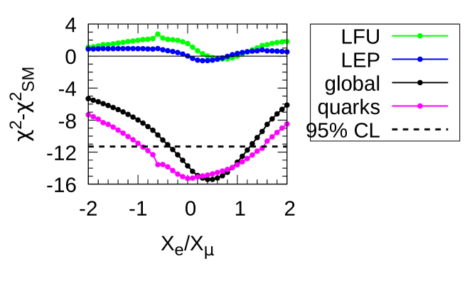
Figure 4: $\chi^{2}$ improvement with respect to that of the SM as a function of electron charge divided by muon charge, $X_{e}/X_{\mu}$. $X_{\tau}=3-X_{e}-X_{\mu}$ at each point, as implied by (21). A negative value of $\chi^{2}-\chi^{2}_{SM}$ indicates an improvement of the fit with respect to the SM whereas a positive value indicates a worse fit than the SM. ‘LFU´ contains 23 observables such as $R_{K}$ and $R_{K^{\ast}}$, which test lepton flavour universality. ‘LEP´ contains the 148 $e^{+}e^{-}\rightarrow l^{+}l^{-}$ measurements discussed in §4. ‘quarks´ contains 224 other $b\rightarrow s\mu^{+}\mu^{-}$ measurements defined in flavio2.3.3. Under the hypothesis that the model line is correct, the region where the ‘global’ results are below the marked dashed line is within the 95$\%$ fit region.

We show the $\chi^{2}$ improvement with respect to the SM in Fig. 4 as a function of the $U(1)_{X}$ electron charge divided by the muon charge, $X_{e}/X_{\mu}$. All fit outputs that we present are approximately only sensitive to this ratio of charges aside from the value of the best-fit gauge coupling $g_{Z^{\prime}}$ and the mixing angle $\theta_{sb}$: these are sensitive to the value of $X_{\mu}$ itself, and shall be presented here for the default value of 10 for this variable. The 23 measurements of LFU observables prefer $X_{e}/X_{\mu}=1$ to values of the ratio that are below 0, where a $\chi^{2}$ of 2 higher than in the SM is evident. The LEP-2 constraints pass through the origin, since $X_{e}=0$ decouples the $Z^{\prime}$ from electron pairs, meaning that the tree-level predicted cross-sections are identical to those of the SM. A ‘LEP´ $\chi^{2}$ contribution of up to 1 higher than that of the SM is possible in the domain $X_{e}/X_{\mu}\in[-2,2]$ best fits. On the other hand, the ‘quarks’ set of observables, which contains angular distributions of $B\rightarrow K^{\star}\mu^{+}\mu^{-}$ decays and of branching ratios in different bins of di-muon invariant mass squared, enjoys a larger effect, improving $\chi^{2}$ on the SM value by over 9 units in the domain taken. Adding all effects together in the ‘global’ fit, we see that in fact $X_{e}/X_{\mu}$ of around 1/2 is preferred. Both $X_{e}=0$ and $X_{\mu}=X_{e}$ are within the 95$\%$ CL preferred region $-0.4<X_{e}/X_{\mu}<1.3$ (however, neither is within the 68$\%$ CL region).

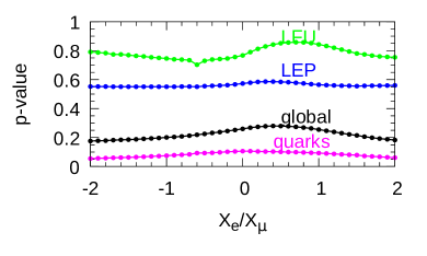
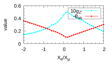
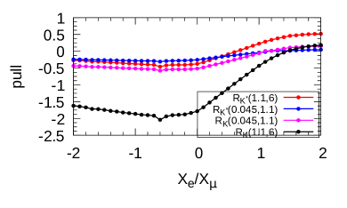
Figure 5: (left panel) $p-$values, (right panel) best-fit parameters for $X_{\mu}=10$ and (bottom panel) 2022 LHCb LFU measurements associated with each model, as a function of $X_{e}/X_{\mu}$, for $M_{Z^{\prime}}=3$ TeV. $X_{\tau}=3-X_{e}-X_{\mu}$ at each point, as implied by (21). In the left panel, ‘LFU´ contains 23 observables (including the aforementioned 2022 LHCb LFU measurements) such as $R_{K}$ and $R_{K^{\ast}}$, which test lepton flavour universality. ‘LEP´ contains the 148 $e^{+}e^{-}\rightarrow l^{+}l^{-}$ measurements discussed in §4. ‘quarks´ contains 224 other $b\rightarrow s\mu^{+}\mu^{-}$ measurements defined in flavio2.3.3. In the bottom panel, the legend displays the domain of invariant mass squared in GeV² in parenthesis and ‘pull’ is defined as $(p-e)/\sigma$, where $p$ is the theoretical prediction of the best-fit point of the $U(1)_{X}$ model, $e$ is the experimental central value and $\sigma$ is the experimental uncertainty, ignoring correlations with other observables.

The $p-$values associated with each fit, as well as the best-fit values of parameters, are displayed in the left-hand panel of Fig. 5. We see that the $p-$values of the three categories defined are all above the .05 level, indicating that no category has a terrible fit. The global $p-$values show a reasonable fit overall in the .15-.26 range throughout the domain of $X_{e}/X_{\mu}$ shown. However, we should bear in mind that the $p-$values have been ‘diluted’ by measurements included in some categories that have large errors (for example some of the Belle data in the ‘LFU’ category). We also see that the ‘quarks’ category is not fit perfectly; this could be due either to: the flavio2.3.3 predictions not having large enough theory errors ascribed to them, unaccounted for experimental systematic errors or that the set of models we have chosen is not the best one to describe the data in the category. In the right-hand panel of Fig. 5, we see some trends. The fact that $g_{Z^{\prime}}$ falls towards the right-hand side and left-hand side of the plot can be seen as due to the fact that LEP constraints will prefer a smaller value of $g_{Z^{\prime}}$ when $|X_{e}|$ is large, since then the $Z^{\prime}$ coupling to electrons is higher. When $g_{Z^{\prime}}$ is smaller, $\theta_{sb}$ is higher. This is expected: since the non-zero tree-level new physics WET WC is constrained by the model to be

$$C_{9}^{(\mu)}=-\frac{X_{\mu}{Q_{3}}}{2}\frac{g_{Z^{\prime}}^{2}}{M_{Z^{\prime}}^{2}}\sin 2\theta_{sb}.$$ (71)

Requiring some particular fixed value of $C_{9}^{(\mu)}\neq 0$ to fit the quarks category, we see that $g_{Z^{\prime}}/M_{Z^{\prime}}$ would tend to move in the opposite direction to $\theta_{sb}$.

The left-hand panel of Fig. 5 confirms that out of our set, globally, $X_{e}/X_{\mu}\approx 1/2$ provides a close-to-optimal fit to the experimental measurements included. The optimal model at this value of the ratio corresponds to fermionic charges of $3B_{3}-5L_{e}-10L_{\mu}+12L_{\tau}$. Some may feel that, aesthetically, some of the charges in this assignment are rather large. This suggests that we investigate a different model in our set with the same ratio of $X_{e}/X_{\mu}$ but with smaller $X_{\mu}$. By adjusting $g_{Z^{\prime}}$, we may expect the fit then to reach a similar $\chi^{2}-\chi^{2}_{SM}$ for the LEP observables. We also expect that $\theta_{sb}$ will then change to keep the value of (71) invariant. There should be only small corrections to this overall $\chi^{2}-$invariant picture from the different gauge coupling affecting the renormalisation between $M_{Z^{\prime}}$ and $M_{Z}$. One charge assignment with $X_{e}/X_{\mu}=1/2$ which is anomaly-free is $3B_{3}-L_{e}-2L_{\mu}$. We shall investigate this model in more detail now.

5.1 $3B_{3}-L_{e}-2L_{\mu}$

Here, we perform a new fit to the $3B_{3}-L_{e}-2L_{\mu}$ model; the result is displayed in Table 3.

	$\chi^{2}-\chi^{2}_{SM}$	$p-$value	measurement	pull
LFU	-0.2	.85	$R_{K^{\ast}}[0.1,\ 1.1]$	-0.1
LEP	-0.4	.58	$R_{K^{\ast}}[1.1,\ 6]$	-1.1
quarks	-14.7	.10	$R_{K}[0.1,\ 1.1]$	-0.3
global	-15.3	.28	$R_{K}[1.1,\ 6]$	-0.1

Table 3: Quality-of-fit for the $3B_{3}-L_{e}-2L_{\mu}$ $Z^{\prime}$ model and the pulls of the 2022 LHCb LFU measurements. The numbers in square parenthesis refer to the end-points of the domain of the relevant bin of di-lepton invariant mass squared, in units of GeV². For $M_{Z^{\prime}}=3$ TeV, the best-fit parameters are $g_{Z^{\prime}}=0.222$, $\theta_{sb}=-0.0270$.

We see that the overall fit is of an acceptable quality, with a $p-$value of .28. The higher invariant mass-squared bin of $R_{K}$ is compatible with its experimental value (the pull is 1.1$\sigma$), whereas the others are all well fit. The $B_{3}-L_{e}-2L_{\mu}$ model has a $\chi^{2}$ improvement of $15.3$ as compared to the SM, for two additional fitted parameters. The $p-$value of the SM being statistically as good a fit to the data as the $B_{3}-L_{e}-2L_{\mu}$ model is .0005.

We display the parameter space of the model in Fig. 6.

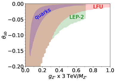
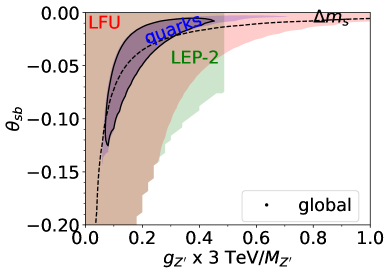
Figure 6: Parameter space of the $3B_{3}-L_{e}-2L_{\mu}$ model: (left) compatibility of different sets of observables and (right) constraints. ‘LFU´ contains 23 observables (including the aforementioned 2022 LHCb LFU measurements) such as $R_{K}$ and $R_{K^{\ast}}$, which test lepton flavour universality. ‘LEP-2´ contains the 148 $e^{+}e^{-}\rightarrow l^{+}l^{-}$ measurements discussed in §4. ‘quarks´ contains 224 other $b\rightarrow s\mu^{+}\mu^{-}$ measurements defined in flavio2.3.3. In the left-hand panel, the coloured regions show where the $p-$value of each labelled constraint is greater than 0.05. In the right-hand panel, the coloured regions are the 95$\%$ confidence limit (CL) allowed regions defined by $\chi^{2}-\chi^{2}(\text{min})=5.99$ James:2004xla as shown for the labelled category of observable. The black line encloses the 95$\%$ CL global region and the black dot gives the locus of the best-fit point. The region above the dashed line is compatible with the $B_{s}-\overline{B_{s}}$ mixing constraint at the 95$\%$ CL (note that this measurement is a member of the ‘quarks’ set of observables).

One should interpret the left-hand panel as testing the joint compatibility of measurements between different categories of observable in the model. We see, since the regions of acceptable fit (defined here to be $p-$value greater than .05) overlap, there is parameter space where each constraint is compatible with every category. The right-hand panel should be interpreted as parameter constraints upon the model, assuming that the $3B_{3}-L_{e}-2L_{\mu}$ model hypothesis is correct. Here, we see that the constraints from the ‘quarks’ category of observable is more-or-less compatible with the LFU constraints. The LEP-2 constraints cut off the global fit contour at the top-right hand side, for larger $g_{Z^{\prime}}/M_{Z^{\prime}}$. The $B_{s}-\overline{B_{s}}$ mixing constraint cuts off the global-fit region at the lower left-hand side. A curved region at the bottom right-hand side of the plot has too large flavour changing effects in general for flavio2.3.3 to return a numerical answer, which explains why some of the constraints (notably from LEP-2) are bounded there. Such regions are highly ruled out by flavour measurements anyway.

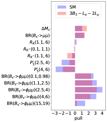
Figure 7: Various pulls of interest for the SM and the best-fit point of the $3B_{3}-L_{e}-2L_{\mu}$ model. Pull is defined as theory prediction minus the experimental central value divided by uncertainty. Correlation between observables is neglected in the calculation of the pull.

We show the pulls of some observables of interest in Fig. 7. We see that although the $3B_{3}-L_{e}-2L_{\mu}$ model fits $B_{s}-\overline{B_{s}}$ mixing (as measured by $\Delta m_{s}$), $BR(B_{s}\rightarrow\mu^{+}\mu^{-})$ and $R_{K^{\ast}}(1.1,6)$ less well than the SM, it ameliorates the fit to more of the other observables. Various bins of $BR(B_{s}\rightarrow\phi\mu^{+}\mu^{-})$, whilst fitting better than in the SM, are still far from optimal (the egregious one being 3$\sigma$ between 2.5 and 4 GeV² in di-muon invariant mass squared). This goes some way to confirming the assertion in the discussion of Fig. 5 that the fit to the ‘quarks’ category of observable, although acceptable, is far from perfect.

6 Conclusion

We have critically re-examined $Z^{\prime}$ models that can significantly ameliorate the $b\rightarrow s\mu^{+}\mu^{-}$ anomalies in global fits. The 2022 re-analysis of the $R_{K}$ and $R_{K^{\ast}}$ observables by LHCb implies that, if the $b\rightarrow s\mu^{+}\mu^{-}$ anomalies are due to beyond the SM effects, there may well also be beyond the SM effects in $b\rightarrow se^{+}e^{-}$. One possible explanation is that of a TeV-scale $Z^{\prime}$ boson that couples dominantly to third family quarks, to $s\bar{b}$ and $b\bar{s}$ through weak mixing effects, to di-muon pairs and to di-electron pairs in addition. We identified a one-rational-parameter family of models which, in the first two-family charged-lepton sector, interpolates between a $Z^{\prime}$ only coupling to di-muon pairs and a $Z^{\prime}$ which couples to di-electron pairs and to di-muon pairs with equal strength. Here, the coupling strength is directly proportional to the $U(1)_{X}$ charge of the leptonic field in question. By coupling a $Z^{\prime}$ to di-electron pairs, one obtains constraints from LEP-2, which measured the scattering of $e^{+}e^{-}$ to di-lepton pairs and observed no significant deviations from SM predictions. One hopefully useful side-product of the present paper was to re-calculate such predicted deviations resulting from relevant dimension-6 SMEFT operators. A previous presentation in the literature Falkowski:2015krw has thus received an independent check. Our calculation is presented in a more complete form than in Ref. Falkowski:2015krw , which guarantees that the resulting predicted LEP-2 cross-sections are positive even in extreme parts of parameter space. The calculations in the more complete form have been programmed into smelli and flavio, and are thus publicly available for use. In a different analysis, other experimental data, such as electroweak precision observables, can be varied (or indeed re-fit) and the LEP-2 constraints will change accordingly in the calculation.

One particular model, $3B_{3}-L_{e}-L_{\mu}-L_{\tau}$, was already examined in Ref. Greljo:2022jac (using the numerical results from a fit to 2015 electroweak and LEP-2 data) where it was found that there is no parameter region where each set of experimental constraints is satisfied to within 1$\sigma$. We think this condition to be overly restrictive and we prefer a global fit strategy. By widening the model space to allow different electron and muon $U(1)_{X}$ charges, we also see how much the preference is for an equal coupling of the $Z^{\prime}$ to di-electron pairs and to di-muon pairs, as compared to some other ratio between the two. This main information is displayed in Fig. 4. From the figure, it appears that zero coupling of the $Z^{\prime}$ boson to di-electron pairs is roughly as good a fit as an equal coupling to di-muon pairs (which is a better fit by only 0.7 units of $\chi^{2}$), globally. We also see from the figure that a $Z^{\prime}$ which couples to di-electron pairs with about half the strength with which it couples to di-muon pairs is a close-to-optimal global fit, at least along one particular line in the space of rational anomaly-free charge assignments. Thus, we are led to propose the $3B_{3}-L_{e}-2L_{\mu}$ model; its properties as regards flavour changing variables are investigated in §5.1. Here, Fig. 5 shows a sub-optimal fit to some observables in the ‘quark’ category of observable, even if the fit to the category as a whole is acceptable. Further lepton-flavour universal corrections to $C_{9}$ WCs coming from non-perturbative corrections may potentially ameliorate these. For more generic models than this close-to-optimal model, the third generation of leptons have a non-zero $U(1)_{X}$ charge of $X_{\mu}+X_{e}-3$ as implied by anomaly cancellation (21). This will have potentially important phenomenological implications, implying a non-zero tree-level new physics contribution to rates for $b\rightarrow s\tau^{+}\tau^{-}$ and affecting the prediction of $b\rightarrow s\bar{\nu}\nu$.

References

- (1) ATLAS Collaboration, M. Aaboud et. al., Study of the rare decays of and mesons into muon pairs using data collected during 2015 and 2016 with the ATLAS detector, JHEP 04 (2019) 098 [1812.03017].
- (2) CMS Collaboration, Measurement of decay properties and search for the decay in proton-proton collisions at , .
- (3) LHCb Collaboration, R. Aaij et. al., Measurement of the branching fraction and effective lifetime and search for decays, Phys. Rev. Lett. 118 (2017), no. 19 191801 [1703.05747].
- (4) CMS Collaboration, Measurement of decay properties and search for the decay in proton-proton collisions at , .
- (5) B. Allanach and J. Davighi, The Rumble in the Meson: a leptoquark versus a Z’ to fit b → s+- anomalies including 2022 LHCb measurements, JHEP 04 (2023) 033 [2211.11766].
- (6) LHCb Collaboration, R. Aaij et. al., Angular analysis and differential branching fraction of the decay , JHEP 09 (2015) 179 [1506.08777].
- (7) CDF Collaboration, Precise Measurements of Exclusive b → sµ+µ Decay Amplitudes Using the Full CDF Data Set, .
- (8) LHCb Collaboration, R. Aaij et. al., Measurement of Form-Factor-Independent Observables in the Decay , Phys. Rev. Lett. 111 (2013) 191801 [1308.1707].
- (9) LHCb Collaboration, R. Aaij et. al., Angular analysis of the decay using 3 fb-1 of integrated luminosity, JHEP 02 (2016) 104 [1512.04442].
- (10) ATLAS Collaboration, M. Aaboud et. al., Angular analysis of decays in collisions at TeV with the ATLAS detector, JHEP 10 (2018) 047 [1805.04000].
- (11) CMS Collaboration, A. M. Sirunyan et. al., Measurement of angular parameters from the decay in proton-proton collisions at 8 TeV, Phys. Lett. B 781 (2018) 517–541 [1710.02846].
- (12) CMS Collaboration, V. Khachatryan et. al., Angular analysis of the decay from pp collisions at TeV, Phys. Lett. B 753 (2016) 424–448 [1507.08126].
- (13) C. Bobeth, M. Chrzaszcz, D. van Dyk and J. Virto, Long-distance effects in from analyticity, Eur. Phys. J. C 78 (2018), no. 6 451 [1707.07305].
- (14) HPQCD Collaboration, W. G. Parrott, C. Bouchard and C. T. H. Davies, Standard Model predictions for B→K+-, B→K1-2+ and B→K¯ using form factors from Nf=2+1+1 lattice QCD, Phys. Rev. D 107 (2023), no. 1 014511 [2207.13371].
- (15) M. Algueró, A. Biswas, B. Capdevila, S. Descotes-Genon, J. Matias and M. Novoa-Brunet, To (b)e or not to (b)e: No electrons at LHCb, 2304.07330.
- (16) Q. Wen and F. Xu, The Global Fits of New Physics in after 2022 Release, 2305.19038.
- (17) J. Aebischer, J. Kumar, P. Stangl and D. M. Straub, A Global Likelihood for Precision Constraints and Flavour Anomalies, Eur. Phys. J. C 79 (2019), no. 6 509 [1810.07698].
- (18) N. Gubernari, M. Reboud, D. van Dyk and J. Virto, Improved theory predictions and global analysis of exclusive processes, JHEP 09 (2022) 133 [2206.03797].
- (19) N. Guberpnari, M. Reboud, D. van Dyk and J. Virto, Dispersive Analysis of and Form Factors, 2305.06301.
- (20) M. Ciuchini, M. Fedele, E. Franco, A. Paul, L. Silvestrini and M. Valli, Constraints on lepton universality violation from rare B decays, Phys. Rev. D 107 (2023), no. 5 055036 [2212.10516].
- (21) G. Isidori, Z. Polonsky and A. Tinari, Semi-inclusive transitions at high , 2305.03076.
- (22) A. J. Buras and E. Venturini, The exclusive vision of rare K and B decays and of the quark mixing in the standard model, Eur. Phys. J. C 82 (2022), no. 7 615 [2203.11960].
- (23) A. J. Buras, Standard Model predictions for rare K and B decays without new physics infection, Eur. Phys. J. C 83 (2023), no. 1 66 [2209.03968].
- (24) LHCb Collaboration, Test of lepton universality in decays, 2212.09152.
- (25) LHCb Collaboration, R. Aaij et. al., Tests of lepton universality using and decays, Phys. Rev. Lett. 128 (2022), no. 19 191802 [2110.09501].
- (26) R. Fleischer, E. Malami, A. Rehult and K. K. Vos, New perspectives for testing electron-muon universality, JHEP 06 (2023) 033 [2303.08764].
- (27) B. Grzadkowski, M. Iskrzynski, M. Misiak and J. Rosiek, Dimension-Six Terms in the Standard Model Lagrangian, JHEP 10 (2010) 085 [1008.4884].
- (28) Heavy Flavor Averaging Group, HFLAV Collaboration, Y. S. Amhis et. al., Averages of b-hadron, c-hadron, and -lepton properties as of 2021, Phys. Rev. D 107 (2023), no. 5 052008 [2206.07501].
- (29) P. Stangl, smelli – the SMEFT Likelihood, PoS TOOLS2020 (2021) 035 [2012.12211].
- (30) R. J. Barlow, Statistics: A Guide to the Use of Statistical Methods in the Physical Sciences. Wiley, 1989.
- (31) N. R. Singh Chundawat, violation in : a model independent analysis, Phys. Rev. D 107 (2023) 075014 [2207.10613].
- (32) J. Davighi, Anomalous Z’ bosons for anomalous B decays, JHEP 08 (2021) 101 [2105.06918].
- (33) C. Bonilla, T. Modak, R. Srivastava and J. W. F. Valle, gauge symmetry as a simple description of anomalies, Phys. Rev. D 98 (2018), no. 9 095002 [1705.00915].
- (34) R. Alonso, P. Cox, C. Han and T. T. Yanagida, Flavoured local symmetry and anomalous rare decays, Phys. Lett. B 774 (2017) 643–648 [1705.03858].
- (35) E. J. Chun, A. Das, J. Kim and J. Kim, Searching for flavored gauge bosons, JHEP 02 (2019) 093 [1811.04320]. [Erratum: JHEP 07, 024 (2019)].
- (36) B. C. Allanach, explanation of the neutral current anomalies, Eur. Phys. J. C 81 (2021), no. 1 56 [2009.02197]. [Erratum: Eur.Phys.J.C 81, 321 (2021)].
- (37) B. C. Allanach and J. Davighi, Third family hypercharge model for and aspects of the fermion mass problem, JHEP 12 (2018) 075 [1809.01158].
- (38) B. C. Allanach and J. Davighi, Naturalising the third family hypercharge model for neutral current -anomalies, Eur. Phys. J. C 79 (2019), no. 11 908 [1905.10327].
- (39) B. Allanach and J. Davighi, helps select models for anomalies, Eur. Phys. J. C 82 (2022), no. 8 745 [2205.12252].
- (40) B. C. Allanach, J. Davighi and S. Melville, An Anomaly-free Atlas: charting the space of flavour-dependent gauged extensions of the Standard Model, JHEP 02 (2019) 082 [1812.04602]. [Erratum: JHEP 08, 064 (2019)].
- (41) B. C. Allanach, B. Gripaios and J. Tooby-Smith, Anomaly cancellation with an extra gauge boson, Phys. Rev. Lett. 125 (2020), no. 16 161601 [2006.03588].
- (42) C. Froggatt and H. Nielsen, Hierarchy of quark masses, cabibbo angles and cp violation, Nuclear Physics B 147 (1979), no. 3 277–298.
- (43) B. C. Allanach, J. E. Camargo-Molina and J. Davighi, Global fits of third family hypercharge models to neutral current B-anomalies and electroweak precision observables, Eur. Phys. J. C 81 (2021), no. 8 721 [2103.12056].
- (44) B. Allanach and E. Loisa, Flavonstrahlung in the B3 L2Z’ model at current and future colliders, JHEP 03 (2023) 253 [2212.07440].
- (45) Particle Data Group Collaboration, R. L. Workman et. al., Review of Particle Physics, PTEP 2022 (2022) 083C01.
- (46) D. M. Straub, flavio: a Python package for flavour and precision phenomenology in the Standard Model and beyond, 1810.08132.
- (47) A. Falkowski and K. Mimouni, Model independent constraints on four-lepton operators, JHEP 02 (2016) 086 [1511.07434].
- (48) A. Greljo, J. Salko, A. Smolkovič and P. Stangl, Rare b decays meet high-mass Drell-Yan, JHEP 05 (2023) 087 [2212.10497].
- (49) I. Brivio and M. Trott, The Standard Model as an Effective Field Theory, Phys. Rept. 793 (2019) 1–98 [1706.08945].
- (50) ALEPH, DELPHI, L3, OPAL, LEP Electroweak Collaboration, S. Schael et. al., Electroweak Measurements in Electron-Positron Collisions at W-Boson-Pair Energies at LEP, Phys. Rept. 532 (2013) 119–244 [1302.3415].
- (51) A. Das, P. S. B. Dev, Y. Hosotani and S. Mandal, Probing the minimal U(1)X model at future electron-positron colliders via fermion pair-production channels, Phys. Rev. D 105 (2022), no. 11 115030 [2104.10902].
- (52) J. Aebischer, J. Kumar and D. M. Straub, Wilson: a Python package for the running and matching of Wilson coefficients above and below the electroweak scale, Eur. Phys. J. C 78 (2018), no. 12 1026 [1804.05033].
- (53) F. James and M. Winkler, MINUIT User’s Guide, 6, 2004. https://inspirehep.net/literature/1258345.