Building Entanglement Entropy out of Correlation Functions for Interacting Fermions

Abstract

We provide a prescription to construct Rényi and von Neumann entropy of a system of interacting fermions from a knowledge of its correlation functions. We show that Rényi entanglement entropy of interacting fermions in arbitrary dimensions can be represented by a Schwinger Keldysh free energy on replicated manifolds with a current between the replicas. The current is local in real space and is present only in the subsystem which is not integrated out. This allows us to construct a diagrammatic representation of entanglement entropy in terms of connected correlators in the standard field theory with no replicas. This construction is agnostic to how the correlators are calculated, and one can use calculated, simulated or measured values of the correlators in this formula. Using this diagrammatic representation, one can decompose entanglement into contributions which depend on the one-particle correlator, two particle correlator and so on. We provide analytic formula for the one-particle contribution and a diagrammatic construction for higher order contributions. We show how this construction can be extended for von-Neumann entropy through analytic continuation. For a practical implementation of a quantum state, where one usually has information only about few-particle correlators, this provides an approximate way of calculating entanglement commensurate with the limited knowledge about the underlying quantum state.

I Introduction

A quantum many body state encodes non-local correlations between degrees of freedom in one part of the system with those in another part; i.e. the information about the state is distributed amongst degrees of freedom which are typically far away from each other. A simple way to see this is to expand a quantum many body state in a basis which is tensor product of local basis states. The complex quantum amplitudes of this expansion (or the many-body wavefunction) store the information about these non-local correlations. The most obvious example of this is quantum statistics: e.g. Fermions cannot share a quantum state, which can impose long range non-local constraints on wavefunctions of many Fermions.

If one is interested in observables which have support only in the Hilbert space of a subsystem $A$, one can trace over the degrees of freedom in the complimentary subsystem $B$ and construct a reduced density matrix (RDM) $\hat{\rho}_{A}$ [1]. This density operator will reproduce all observables in the subsystem and has the usual interpretation of a “classical” ensemble of quantum states as specified by its spectral decomposition. If the RDM represents a pure quantum state in the subsystem, the original state is separable, otherwise it is entangled [2].

Entanglement and its related measures have played an important role in wide ranging fields including quantum information and computation [3, 4], foundations of quantum mechanics [5, *BELL_RMP66_ProblemHiddenVariables, *Clauser.Holt_PRL69_ProposedExperimentTest, *Zeilinger_RMP99_ExperimentFoundationsQuantum], black-hole physics and quantum gravity [9, *hayden_J.HighEnergyPhys.2007_BlackHolesMirrors, *susskind_EREPR, *penington_J.HighEnerg.Phys.2020_EntanglementWedgeReconstruction, *Das:2020xoa], and quantum condensed matter systems [14, 15]. An important measure of entanglement is the bipartite entanglement entropy (EE), which is the classical entropy corresponding to the probability distribution specified by the eigenvalues of $\hat{\rho}_{A}$. In quantum many body systems, the scaling of EE with subsystem size is used to fingerprint states  [16, 15, 17, *Calabrese_2004, *Calabrese_2009, 20, 21], detect presence of topological order  [22, *levin_Phys.Rev.Lett.2006_DetectingTopologicalOrder, *jiang_NaturePhys2012_IdentifyingTopologicalOrder] or occurrence of quantum phase transitions  [25, *SubirON, *SubirWitczakKrempa, *ju_Phys.Rev.B2012_EntanglementScalingTwodimensional]. In fact, exotic states like spin liquids[29] are often best described by the “entanglement patterns” in the ground state  [30, *isakov_NaturePhys2011_TopologicalEntanglementEntropy, *pretko_Phys.Rev.B2016_EntanglementEntropyQuantum]. More recently the entanglement scaling of excited states in the middle of the spectrum [33] has been used to classify whether a disordered interacting system is in an ergodic phase, where local observables can be described by usual statistical mechanics, or in a many body localized phase [34], where laws of statistical mechanics fail to apply. The question of thermalization [35] in a system has also been tracked through the time evolution of entanglement under non-equilibrium dynamics  [36, 37, 38]. Thermalizing systems show a linear growth of entanglement, while many body localized systems have a slower logarithmic growth of entanglement [39, 40]. The growth of entanglement has also played a crucial role in the development of ideas related to quantum chaos [41, *Swingle.Hayden_PRA16_MeasuringScramblingQuantum, 43]. Experimental measurements of EE in many body systems have been performed on a variety of platforms including ion traps [44, 45], ultracold Rydberg atoms [46, 47], and superconducting qubits [48].

There are only a few methods to calculate the EE in interacting many body systems, either in thermal or in the ground state. Even fewer methods can tackle non-equilibrium dynamics of EE. The most direct method is to obtain the quantum state by exact diagonalization, calculate the reduced density matrix and hence the EE [49, 50]. While this is the most widely used method, it is limited to small finite size systems in one dimension, since the specification of a quantum many body state requires knowledge of an exponentially large (in system size) number of quantum amplitudes. Quantum Monte Carlo based methods have been extensively used for systems in one and two dimensions  [51, *Grover_PRL13_EntanglementInteractingFermions, *McMinis.Tubman_PRB13_RenyiEntropyInteracting, *Drut.Porter_PRB15_HybridMonteCarlo]. In the cases where EE is expected to have a weak scaling with system size, numerical techniques using Density Matrix Renormalisation Group ideas [55, *Schollwock_AoP11_DensitymatrixRenormalizationGroup] in one dimension and tensor network based methods [57, *Evenbly.Vidal_JSP11_TensorNetworkStates] in higher dimensions have been used to calculate EE. For non-interacting systems or integrable systems, progress can be made using specialized numerical techniques, as one can reduce the complexity of the calculation [59, *Peschel_2009]. Standard field theoretic techniques for calculation of entanglement entropy [18, *Calabrese_2009, 21] use replica methods with complicated boundary conditions. This limits their scope as it is often impossible to obtain solutions of even simple problems with the complicated boundary conditions. For 1+1 dimensional CFTs [17, *Calabrese_2004], where correlators are tightly constrained, one can obtain exact analytical answers for leading and subleading scaling of EE.

A key problem is calculating EE of a state is the following: we have an operational prescription to calculate EE if we know the exact quantum state; however for a generic system, there is no such prescription to calculate the EE in terms of the correlation functions. There are two aspects to this issue: (a) A prescription to obtain entanglement from correlators can lead to efficient estimates of entanglement in numerics, since efficient algorithms to calculate correlation functions already exist in the literature [61, 56]. There are also a large class of analytic approximation schemes [62, 63] for calculating interacting correlation functions, which have been developed over the years. With a prescription connecting correlations to EE, these methods can increase the scope of study of entanglement in large quantum systems. We note that in the special cases where this prescription is known, like in non-interacting systems [60, 20] or 1+1D CFT [19], our knowledge of EE is vastly more advanced than the cases where such a prescription is not known. (b) In any realistic situation, it is impossible to know the exact quantum state; however there are experimental probes to obtain information about the correlation functions [64]. Even in highly controllable systems like ultracold atoms [65], experiments can at best have knowledge of few-body correlations [66, 67, 68]. A prescription to calculate entanglement entropy from knowledge of correlation functions would thus not only enhance the theoretical space for such calculations, it will be the only consistent description of realistic experimental situations. Here we would like to note that if one requires the knowledge of all $m$-body correlators in a system to calculate EE, the complexity of the problem is same as knowing the full quantum state. Thus it would be useful to have estimates of entanglement which involve only few body correlators, and one should be able to improve these estimates if information about higher order correlators become available.

In this paper, we take on the task of constructing an operational prescription for computing EE of a generic interacting Fermionic system in terms of its correlation functions. We consider the system to be made of mutually exclusive regions $A$ and $B$, with a Hilbert space which is a tensor product of Hilbert spaces for degrees of freedom in $A$ and $B$. We are interested in the EE of the system when the degrees of freedom in $B$ are traced out. We use Schwinger Keldysh field theory [69, 70], which allows us to consider ground states, thermal systems, and closed and open quantum systems evolving in time out of thermal equilibrium on the same footing. Our prescription is agnostic to these different situations. (i) We show that the $n$^th Rényi entropy, $S^{(n)}$, of a system of interacting Fermions is the Schwinger Keldysh free energy of a system of $n$ replicas with “inter-replica currents” flowing only in the subsystem $A$. These currents are local in space (i.e. between same lattice sites, or same location) and in time (currents are present only at the time of measurement). The matching of fields across replica-s in standard field theory technique for calculating EE is replaced by the inter-replica currents in our formalism. We argue that the doubling of fields in the SK field theory is a crucial ingredient which allows boundary conditions to be replaced by quadratic current-like terms, and we do not know of any method which can achieve this in a single contour Lorentzian or Euclidean field theory. (ii) Using this identification of EE with a free energy, we provide a prescription to calculate it in terms of correlations in a single replica theory, which does not involve complicated boundary conditions (it has the same boundary conditions as the usual field theory). (iii) We show that if one only has information of up to $m$-particle connected correlators, one can construct an estimate of EE, which can be improved if information about $m+1$-particle correlators become available. More precisely, for the $n$^th order Rényi Entanglement Entropy (REE), $S^{(n)}$, we show

$$S^{(n)}=S^{(n)}_{1\mathrm{P}}+S^{(n)}_{2\mathrm{P}}+S^{(n)}_{3\mathrm{P}}+\cdots,$$ (1)

where $S^{(n)}_{m\mathrm{P}}$ involves up to $m$-particle connected correlators, $G^{(m)}_{c}$, and does not involve any correlators of higher order (particle number). For $m>1$, $G^{(m)}_{c}$ is simply related to the connected part of the expectation value of a normal ordered string of Fermion operators ($\hat{c}^{\dagger},\hat{c}^{\vphantom{\dagger}}$) w.r.to the state,

$$G^{(m)}_{c}\sim\expectationvalue*{\,\underbrace{\hat{c}^{\dagger}\hat{c}^{\dagger}\cdots\hat{c}^{\dagger}}_{m\rm\ times}\,\underbrace{\hat{c}^{\vphantom{\dagger}}\,\hat{c}^{\vphantom{\dagger}}\,\cdots\hat{c}^{\vphantom{\dagger}}}_{m\rm\ times}\,}_{c}.$$ (2)

We calculate $S^{(n)}_{1\mathrm{P}}$ exactly and provide a prescription of Feynman diagrams for calculating $S^{(n)}_{m\mathrm{P}}$ for $m>1$ in terms of higher order connected correlators. This decomposition would be most useful when the state of the system is close to that of a Gaussian theory (this could be a symmetry broken mean field theory) and higher order connected correlators are parametrically smaller. (iv) The von-Neumann entropy, $S$, does not have a simple field theoretic interpretation, but has to be calculated as an analytic continuation of REE, i.e. $S=\lim_{n\to 1}S^{(n)}$. We posit a similar $m$-particle decomposition for $S$,

$$S=S_{1\mathrm{P}}+S_{2\mathrm{P}}+S_{3\mathrm{P}}+\cdots,$$ (3)

where $S_{m\mathrm{P}}=\lim_{n\to 1}S^{(n)}_{m\mathrm{P}}$. We calculate $S_{1\mathrm{P}}$ exactly, and show that a large class of diagrams for $S^{(n)}_{m\mathrm{P}}$ vanish when the $n\to 1$ limit is taken. For $S_{2\mathrm{P}}$, we explicitly calculate the first non-trivial diagram which involves two 2-particle connected correlators. Note that our prescription is completely agnostic to how the connected correlation functions are calculated. Our formulation thus opens up the possibility of computing EE using approximate analytic techniques, numerically obtained correlators or even experimentally measured ones. We believe this construction will allow large scale calculations of EE in higher dimensions ( $d>1$) both in and out of equilibrium.

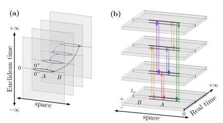
Figure 1: Replica based evaluation of $S^{(4)}$ : (a) Standard technique for ground states where the reduced density matrix is represented as a Euclidean-time path integral with boundary conditions in the subsystem $A$. The fields are matched across consecutive replica as shown. (b) Our formalism expresses each replica of the density matrix on a real time Keldysh contour with doubled fields. Fields at each point of the subsystem $A$ in one replica are coupled to their counterparts in all other replicas. For $S^{(4)}$ this implies coupling between sheet $1$ and $3$, and between sheet $2$ and $4$, in addition to the coupling between consecutive ones. The coupling operates only at the time of observation $t_{o}$, and is “directional” in Replica space, acting as a “Replica current”. Partial tracing is achieved by setting the coupling to zero in the complementary subsystem $B$. No field matchings are required in this new formalism.

The remainder of the text is organised as follows. In Section II we establish that the $n$^th order REE for a generic system of interacting fermions is equal to the Schwinger Keldysh free energy of $n$ replicas of the system coupled via inter-replica currents. We use this fact in Section III to show how $S^{(n)}$ can be decomposed into $m$ particle contributions $S^{(n)}_{m\mathrm{P}}$ and provide explicit diagrammatic rules to construct the same in terms of $k$ particle correlators with $1\leq k\leq m$. Section IV is devoted to the analytic continuation of these contributions as $n\to 1$. In Section V we provide an alternate diagrammatic prescription in terms of Green’s functions of the non-interacting replicas in presence of the quadratic inter-replica current terms. These correlators depend on replica indices and do not admit the usual physical interpretations as correlators in standard Keldysh filed theory. Lastly we conclude in Section VI with a summary of our findings.

II Entanglement Entropy as a Free Energy in presence of Replica Currents

Consider a system of Fermions which is made up of two mutually exclusive spatial subsystems $A$ and $B$. For our purpose, we consider a lattice with $V$ sites, where the subsystem $A$ has $V_{A}$ sites. We will explicitly work with discrete lattice systems, and take appropriate continuum limit at the end. The Hilbert space of the system is a product of the Hilbert space of degrees of freedom lying in A and those lying in B, i.e. ${\cal H}_{AB}={\cal H}_{A}\otimes{\cal H}_{B}$. On tracing over degrees of freedom in $B$, a quantum state of the full system, $\ket{\psi(t_{o})}$ gives rise to a reduced density matrix $\hat{\rho}_{A}(t_{o})$ over the subsystem $A$. Here $t_{o}$ is the time of observation. The $n^{{\text{th}}}$ order Rényi entanglement entropy (REE) of this state for the partition between $A$ and $B$ is then given by

$$S^{(n)}(t_{o})=-\frac{1}{n-1}\ln\Tr[\left(\hat{\rho}_{A}(t_{o})\right)^{n}],$$ (4)

while the von-Neumann entanglement entropy (referred to as EE in the following) is obtained as the analytic continuation

$$S(t_{o})=\lim_{n\to 1}S^{(n)}(t_{o})=-\Tr[\hat{\rho}_{A}(t_{o})\ln\hat{\rho}_{A}(t_{o})].$$ (5)

In a steady state or in equilibrium, the RDM and hence the entropies are independent of $t_{o}$. In the standard field theoretic prescription for calculation of $S^{(n)}$, one considers $n$ copies(replicas) of the system. The time evolution of each of these replicas can be written as a functional integral over fields, giving rise to $n$ fields for each space-time point. The multiplication of RDMs translates to imposing the boundary condition that the fields within subsystem $A$ in different replicas have to be matched at the time of measurement. A schematic representation of this prescription is shown in Fig. 1(a). This naturally leads to integrals over constrained field configurations in the replica space [19]. Here, we propose a modified scheme (schematically shown in Fig. 1(b)) to calculate REE of fermions which uses Schwinger Keldysh field theory for $n$ replicas [37, 71, 38, 72, 73]. The key advantage is that we can trade the boundary conditions in favour of “currents” flowing between replicas in the subsystem A. This allows us to connect REE with standard correlators of the original non-replicated theory.

To develop our formalism, it is useful to define the Wigner characteristic $\chi$ of a density matrix, as the expectation value of the fermionic displacement operator [74, 75, 38],

$$\chi({\bm{\bar{\zeta}}},{\bm{\zeta}};t_{o})=\Tr[\hat{\rho}(t_{o})\,\mathrm{e}^{\sum_{i}\hat{c}^{\dagger}_{i}\zeta_{i}-\bar{\zeta}_{i}\hat{c}^{\vphantom{\dagger}}_{i}}],$$ (6)

where $\hat{\rho}(t_{o})$ is the density matrix of the full system. The Wigner characteristic has the useful property that $\chi$ for the RDM is given by

$$\chi_{A}({\bm{\bar{\zeta}}},{\bm{\zeta}};t_{o})=\Tr[\hat{\rho}(t_{o})\,\mathrm{e}^{\sum_{i\in A}\hat{c}^{\dagger}_{i}\zeta_{i}-\bar{\zeta}_{i}\hat{c}^{\vphantom{\dagger}}_{i}}],$$ (7)

i.e. one simply needs to restrict the support of the displacement operator to ${\cal H}_{A}$ [37]. From now onwards we will use ${\bm{\zeta}}$ and ${\bm{\eta}}$ to indicate vectors of Grassmann variables with support only in $A$. Note that $\chi_{A}$ is a Grassmann valued function of the Grassmann fields $\zeta_{i},\bar{\zeta}_{i}$ and does not have an immediate physical interpretation. Its usefulness lies in the fact that expectations values of operators with support in $A$ can be written as integrals over $\chi$,

$$\expectationvalue*{\hat{O}}[t_{o}]\equiv\Tr[\hat{\rho}_{A}(t_{o})\hat{O}]=2^{-V_{A}}\int\mathcal{D}\left[{\bm{\bar{\zeta}}},{\bm{\zeta}}\right]\mathcal{D}\left[{\bm{\bar{\eta}}},{\bm{\eta}}\right]\,\chi_{A}\left(\sqrt{2}{\bm{\bar{\eta}}},\sqrt{2}{\bm{\eta}};\,t_{o}\right)\chi_{O}\left(\sqrt{2}{\bm{\bar{\zeta}}},\sqrt{2}{\bm{\zeta}}\right)e^{{\bm{\bar{\zeta}}}\cdot{\bm{\eta}}-{\bm{\bar{\eta}}}\cdot{\bm{\zeta}}},$$ (8)

where $\chi_{O}\left({\bm{\bar{\zeta}}},{\bm{\zeta}}\right)=\Tr[\hat{O}\leavevmode\nobreak\ \,\mathrm{e}^{\sum_{i\in A}\hat{c}^{\dagger}_{i}\zeta_{i}-\bar{\zeta}_{i}\hat{c}^{\vphantom{\dagger}}_{i}}]$ is the Weyl symbol of the operator $\hat{O}$ and the dot product ${\bm{\bar{\zeta}}}\cdot{\bm{\eta}}=\sum_{i\in A}\bar{\zeta}_{i}\eta_{i}$. It is then easy to see (substituting $\hat{\rho}_{A}$ for $\hat{O}$) that the $2^{\text{nd}}$ Rényi entropy is given by

$$e^{-S^{(2)}(t_{o})}=2^{-V_{A}}\int\mathcal{D}\left[{\bm{\bar{\zeta}}},{\bm{\zeta}}\right]\mathcal{D}\left[{\bm{\bar{\eta}}},{\bm{\eta}}\right]\chi_{A}\left(\sqrt{2}{\bm{\bar{\eta}}},\sqrt{2}{\bm{\eta}};\,t_{o}\right)\chi_{A}\left(\sqrt{2}{\bm{\bar{\zeta}}},\sqrt{2}{\bm{\zeta}};\,t_{o}\right)e^{{\bm{\bar{\zeta}}}\cdot{\bm{\eta}}-{\bm{\bar{\eta}}}\cdot{\bm{\zeta}}}.$$ (9)

Using properties of displacement operators and fermionic coherent states, Ref. [38] showed that the $n$^th order REE corresponding to can be written as (suppressing the time index),

$$\begin{split}\,\mathrm{e}^{-(n-1)S^{(n)}}=2^{-{(n-1)}V_{A}}\int\prod_{\alpha=1}^{n-1}\mathcal{D}\left[{\bm{\bar{\zeta}}}^{(\alpha)},{\bm{\zeta}}^{(\alpha)}\right]\mathcal{D}\left[{\bm{\bar{\eta}}}^{(\alpha)},{\bm{\eta}}^{(\alpha)}\right]\leavevmode\nobreak\ \prod_{\alpha=1}^{n-1}\chi_{A}\left(\sqrt{2}{\bm{\bar{\eta}}}^{(\alpha)},\sqrt{2}{\bm{\eta}}^{(\alpha)}\right)\leavevmode\nobreak\ \chi_{A}\left(\sqrt{2}\sum\nolimits_{\alpha}{\bm{\bar{\zeta}}}^{(\alpha)},\sqrt{2}\sum\nolimits_{\alpha}{\bm{\zeta}}^{(\alpha)}\right)\\ \exp\left({\sum_{\alpha=1}^{n-1}{\bm{\bar{\zeta}}}^{(\alpha)}\!\cdot{\bm{\eta}}^{(\alpha)}-{\bm{\bar{\eta}}}^{(\alpha)}\!\cdot{\bm{\zeta}}^{(\alpha)}+\sum_{\alpha>\beta}{\bm{\bar{\zeta}}}^{(\alpha)}\!\cdot{\bm{\zeta}}^{(\beta)}-{\bm{\bar{\zeta}}}^{(\beta)}\!\cdot{\bm{\zeta}}^{(\alpha)}}\right).\end{split}$$ (10)

Here $1\leq\alpha,\beta\leq n-1$ are replica indices. Note that while there are product of $n$ replicas, the integration is over $2(n-1)$ pairs of Grassmann variables for each site in $A$.

Eq. (10) is the starting point of our attempt to find a field theoretic construction of EE and hence a general relation between correlators and entanglement. For this, we work with the Schwinger Keldysh field theory of Fermions[69], which describes the evolution of a many body density matrix $\hat{\rho}(t)=\hat{U}(t,0)\hat{\rho}(0)\hat{U}^{\dagger}(t,0)$ in terms of path/functional integrals over two Fermionic (Grassmann) fields $\psi_{\pm}(i,t)$ at each space-time point. The $\psi_{+}$ fields are obtained from the expansion of $\hat{U}$ (i.e. forward propagation of states) while the $\psi_{-}$ fields come from the expansion of $\hat{U}^{\dagger}$ (i.e. backward propagation of states), giving ’rise to a field theory on a closed contour. The partition function $\mathcal{Z}$ on this contour in presence of sources $J_{\pm},\bar{J}_{\pm}$ is

$$\mathcal{Z}[\bar{J}_{\pm},J_{\pm}]=\!\int\!\mathcal{D}\left[\bar{\psi}_{\pm},\psi_{\pm}\right]\!\,\mathrm{e}^{\iota\mathcal{S}_{K}[\bar{\psi}_{\pm},\psi_{\pm}]+\iota\!\int\differential{t}\bar{J}_{+}\psi_{+}-\bar{J}_{-}\psi_{-}+{\text{h.c.}}},$$

where the Keldysh action $\mathcal{S}_{K}$ determines the evolution of the correlators in the system. Note that although we have used the same notation $\mathcal{D}\left[\cdot\right]$ to indicate integrals over the Fermion matter fields $\psi$ as well as integrals over the arguments of the Wigner characteristic ($\zeta,\eta$), the matter fields fluctuate in space-time, while the arguments of Wigner characteristic are evaluated at $t_{o}$ and hence have only spatial variations. In this section, we do not need specific forms of the action, and will refrain from talking about them. One obvious advantage of using a Keldysh field theory is that one can treat both equilibrium and non-equilibrium situations in the same footing.

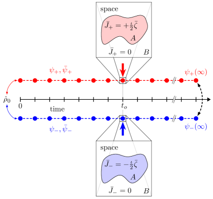
Figure 2: Schematic representation of the Wigner characteristic function $\chi_{A}({\bm{\bar{\zeta}}},{\bm{\zeta}};t_{o})$ as a Keldysh path integral with source insertions. Expanding the evolution operators $\hat{U}(t,0)$ and $\hat{U}^{\dagger}(t,0)$ leads to a path integral with fields on the “forward”(red) and “backward”(blue) contours respectively. The fields are identified at $t=\infty$ and are connected at $t=0$ through the matrix elements of the initial density matrix $\hat{\rho}_{0}$. The displacement operator is inserted symmetrically on both forward and backward contours at the time of observation $t_{o}$ and is equivalent to insertion of sources $J_{\pm},\bar{J}_{\pm}$. The call-out shows the spatial distribution of these sources; they take nonzero values only in subsystem $A$.

In earlier works [38, 71, 37], we had shown that the Wigner characteristic of the reduced density matrix is the Schwinger-Keldysh partition function of the system in presence of sources which couple to fields in the subsystem $A$ only at the time when the entropy is measured, i.e. $\bar{J}_{\pm}(i,t)=\pm\,\iota\,\bar{\zeta}_{i}/2\,\delta(t-t_{o})$ if $i\in A$ and $0$ otherwise. This is schematically shown in Fig. 2. Note that the partition function automatically traces over degrees of freedom in $B$, the sources are inserted in $A$ to compute the Wigner characteristic.

At this point, it will be useful to shift to symmetric ($\psi_{\text{s}},\bar{\psi}_{\text{s}}$) and antisymmetric ($\psi_{\text{a}},\bar{\psi}_{\text{a}}$) combinations of the $\pm$ fields defined at each spacetime point as,

$$\psi_{\text{s}} =(\psi_{+}+\psi_{-})/\sqrt{2},\quad \bar{\psi}_{\text{s}} =(\bar{\psi}_{+}+\bar{\psi}_{-})/\sqrt{2},$$

$$\psi_{\text{a}} =(\psi_{+}-\psi_{-})/\sqrt{2},\quad \bar{\psi}_{\text{a}} =(\bar{\psi}_{+}-\bar{\psi}_{-})/\sqrt{2}.$$

The symmetric source $J_{\text{s}}=(J_{+}+J_{-})/\sqrt{2}$ couples to the antisymmetric field $\bar{\psi}_{\text{a}}$, while the antisymmetric source $J_{\text{a}}=(J_{+}-J_{-})/\sqrt{2}$ couples to the symmetric field $\bar{\psi}_{\text{s}}$. For the Wigner characteristic, the source structure works out to

$$\left.\begin{aligned} J_{\text{s}}(i,t)&=0,\quad&J_{\text{a}}(i,t)&=-\tfrac{\iota}{\sqrt{2}}\zeta_{i}\delta(t-t_{o}),\\ \bar{J}_{\text{s}}(i,t)&=0,\quad&\bar{J}_{\text{a}}(i,t)&=\tfrac{\iota}{\sqrt{2}}\bar{\zeta}_{i}\delta(t-t_{o})\end{aligned}\right\}{\text{ for {\hbox{i \in A}},}}$$ (11)

and $0$ otherwise. We can then write

$$\chi_{A}(\sqrt{2}{\bm{\bar{\zeta}}},\sqrt{2}{\bm{\zeta}},t_{o})$$ (12)

$$=\!\!\int\mathcal{D}\left[{\bm{\bar{\psi}}}_{\text{s,a}},{\bm{\psi}}_{\text{s,a}}\right]\,\mathrm{e}^{\iota\mathcal{S}_{K}[{\bm{\bar{\psi}}}_{\text{s,a}},{\bm{\psi}}_{\text{s,a}}]+{\bm{\bar{\zeta}}}\cdot\hat{P}_{A}{\bm{\psi}}_{\text{s}}(t_{o})-{\bm{\bar{\psi}}}_{\text{s}}(t_{o})\hat{P}_{A}\cdot{\bm{\zeta}}},$$

where $\hat{P}_{A}$ is a projection operator on to the degrees of freedom in subsystem $A$, added to explicitly account for the sources coupling only to the degrees of freedom in $A$. Substituting Eq. (12) into Eq. (10), we obtain

$$\,\mathrm{e}^{-(n-1)[S^{(n)}-V_{A}\ln 2]}=\int\prod_{\alpha=1}^{n}\mathcal{D}\left[{\bm{\bar{\psi}}}^{(\alpha)}_{\text{s,a}},{\bm{\psi}}^{(\alpha)}_{\text{s,a}}\right]\,\mathrm{e}^{\iota\sum\nolimits_{\alpha=1}^{n}\mathcal{S}_{K}\left[{\bm{\bar{\psi}}}^{(\alpha)}_{\text{s,a}},{\bm{\psi}}^{(\alpha)}_{\text{s,a}}\right]}\,\mathrm{e}^{\iota\mathcal{S}_{\text{ent}}\left[\left\{\hat{P}_{A}{\bm{\bar{\psi}}}_{\text{s}}^{(\alpha)}(t_{o}),\hat{P}_{A}{\bm{\psi}}_{\text{s}}^{(\beta)}(t_{o})\right\}\right]},$$ (13)

where the entangling action, $\mathcal{S}_{\text{ent}}$, is given by

$$\,\mathrm{e}^{\iota\mathcal{S}_{\text{ent}}} =\int\prod_{\alpha=1}^{n-1}\mathcal{D}\left[{\bm{\bar{\zeta}}}^{(\alpha)},{\bm{\zeta}}^{(\alpha)},{\bm{\bar{\eta}}}^{(\alpha)},{\bm{\eta}}^{(\alpha)}\right]\exp\left({\sum_{\alpha=1}^{n-1}{\bm{\bar{\zeta}}}^{(\alpha)}\!\cdot{\bm{\eta}}^{(\alpha)}-{\bm{\bar{\eta}}}^{(\alpha)}\!\cdot{\bm{\zeta}}^{(\alpha)}+\sum_{\alpha>\beta}{\bm{\bar{\zeta}}}^{(\alpha)}\!\cdot{\bm{\zeta}}^{(\beta)}-{\bm{\bar{\zeta}}}^{(\beta)}\!\cdot{\bm{\zeta}}^{(\alpha)}}\right)$$ (14)

$$\hphantom{=\int\prod_{\alpha=1}^{n-1}}\exp\left({\sum_{\alpha=1}^{n-1}{\bm{\bar{\eta}}}^{(\alpha)}\!\cdot\hat{P}_{A}{\bm{\psi}}_{\text{s}}^{(\alpha)}(t_{o})-{\bm{\bar{\psi}}}^{(\alpha)}_{\text{s}}(t_{o})\hat{P}_{A}\!\cdot{\bm{\eta}}^{(\alpha)}}+{\sum_{\alpha=1}^{n-1}{\bm{\bar{\zeta}}}^{(\alpha)}\!\cdot\hat{P}_{A}{\bm{\psi}}_{\text{s}}^{(n)}(t_{o})-{\bm{\bar{\psi}}}^{(n)}_{\text{s}}(t_{o})\hat{P}_{A}\!\cdot{\bm{\zeta}}^{(\alpha)}}\right).$$

The first part of Eq. (13) represents the action of $n$ independent replicas, while the entangling action involves integrals over the source terms in each of the replicas. Note that in absence of $\mathcal{S}_{\text{ent}}$, the Keldysh partition function of the independent replicas is $1$, and hence the entanglement would have vanished, i.e. the finite entanglement comes solely from the effects of $\mathcal{S}_{\text{ent}}$. This is consistent with the fact that $\mathcal{S}_{\text{ent}}$ has information about the subsystem $A$, since the sources are restricted to $A$. While this may seem similar to the standard path integral over $n$ replicas used in field theoretic treatment of entanglement [21, 19], we note that we have $2n$ fields here. Beyond the obvious fact that this allows us to look at non-equilibrium dynamics, we will see that even for equilibrium systems or ground states, using $2n$ fields gives us certain advantages in terms of the structure of the resultant theory.

For a non-interacting system, with Gaussian action, both the integrals over the fields and the sources can be performed exactly (in either order); however for a generic interacting system, it is not possible to integrate out the matter fields exactly. Fortunately, even in this case, the integral over the sources is just a Gaussian integral, which can be done analytically to get

$$\iota\mathcal{S}_{{\text{ent}}}=\begin{bmatrix}{\bm{\bar{\psi}_{\text{s}}}}^{(1)},{\bm{\bar{\psi}_{\text{s}}}}^{(2)},\cdots,{\bm{\bar{\psi}_{\text{s}}}}^{(n)}\end{bmatrix}\mathbb{J}\otimes\hat{P}_{A}\begin{bmatrix}{\bm{\psi_{\text{s}}}}^{(1)}\\ {\bm{\psi_{\text{s}}}}^{(2)}\\ \vdots\\ {\bm{\psi_{\text{s}}}}^{(n)}\end{bmatrix},$$ (15)

where $\mathbb{J}$ is an $n\times n$ antisymmetric matrix with all entries below the diagonal equal to one,

$$\mathbb{J}=\begin{pmatrix}\hphantom{-}0&-1&\hphantom{-}\cdots&-1\\ \hphantom{-}1&\hphantom{-}0&\hphantom{-}\ddots&\hphantom{-}\vdots\\ \hphantom{-}\vdots&\hphantom{-}\ddots&\hphantom{-}\ddots&-1\\ \hphantom{-}1&\hphantom{-}\cdots&\hphantom{-}1&\hphantom{-}0\end{pmatrix}_{n\times n}.$$ (16)

Note that the integral over the sources couples the fields in different replicas in $\mathcal{S}_{\text{ent}}$. It is useful to note the following features of the entangling action:

• The integration of sources produces a replica coupling term which is quadratic in the fields and only couples fields in the subsystem $A$ across replicas.

• The coupling is local in space and time, i.e. it connects fields on the same lattice sites, only at the time of measuring the REE.

• The structure of $\mathcal{S}_{\text{ent}}$ has the form of a “current” in the replica space, flowing between the same sites in the subsystem $A$ across any two distinct replicas. The entangling action does not couple fields in the same replica, but couples fields in all distinct replica pairs. In contrast, the standard replica trick with Euclidean field theory involves fields in one replica being identified with their counterparts in consecutive replicas. The schematic difference between the standard approach and our approach is shown in Fig. 1(a) and (b). The use of the two-contour SK field theory allows the replacement of the boundary condition by quadratic terms. The boundary condition in standard replica methods requires one to work with actions defined on $n$-sheeted Riemann surfaces for generic interacting systems, with reduction to a single sheet possible in special cases, like in free theories  [21] or in presence of conformal symmetry in $1+1$D  [19]. Our formalism on the other hand, involves “current”-like couplings between replicas without additional boundary conditions on fields across replicas. This will allow us to write down a diagrammatic expansion for EE in terms of the local connected correlators of the single replica for a generic theory. We will take up this task in the next section.

• It is important to note that the Keldysh indices of the fields making up the entangling action has the form $\sim\bar{\psi}^{(\alpha)}_{\text{s}}\psi^{(\beta)}_{\text{s}}$ with $\alpha\neq\beta$. Such a term involving fields from the same replica is forbidden in usual Schwinger Keldysh field theory as it would change normalization of $\hat{\rho}$ and affect the causal structure of the correlations. Thus there is no obvious analogue of this term in usual single component field theories, or thermal field theories. The doubling of the fields in the Keldysh formalism is what allows us to write this term, even if we are considering the entanglement of a thermal state or a ground state. Thus, Keldysh field theory is not just a way to access non-equilibrium dynamics in this case, it is essential to writing down a space-time local description of entanglement entropies.

• Finally we would like to note that the equations derived till now are agnostic to the explicit form of the action. For e.g., they do not require conformal invariance, and can be used for generic interacting systems in any dimension both in and out of equilibrium.

Thus the $n$^th order REE is the Keldysh free energy of the $n$-fold replicated system in presence of the inter-replica “current” between the same sites in the subsystem $A$. These currents are active only at the time of measurement of the entropy of the system. For a system in ground state/ thermal equilibrium / steady state, the entropy is independent of the time of measurement, and we can choose the time to simplify calculations. For non-equilibrium dynamics, which tracks the time evolution of entanglement entropy, one is interested in calculating the entropy as a function of the measurement time $t_{o}$. We have thus provided an alternate field theoretic picture of REE of fermionic systems. We note that a similar construction for Bosonic systems runs into issues of zero modes, and we will take it up in a future work [73].

III Feynman Diagrams and “m” particle Entanglement

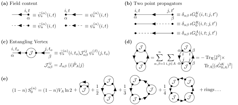
Figure 3: Diagrammatic representation of (a) the symmetric($\psi_{\text{s}}$) and antisymmetric($\psi_{\text{a}}$) fields in the theory, (b) the two point propagators of the free theory in each replica, and (c) the entangling vertex (for details about vertex factors refer to main text, Eq. (15) & Eq. (16)). Lattice sites are labelled by $i,j$ and $1\leq\alpha,\beta\leq n$ are replica indices. (d) A ring diagram with two $\cal J$ vertices. We explicitly evaluate the diagram with lattice and replica indices marked on each propagator. Since the latter are same in each replica, the resulting sum factorises into a trace over replica indices ($\cal R$), and a trace over the subsystem ($A$). (e) Rényi entropy in a free theory, $S^{(n)}_{0}$, is the sum of all ring diagrams. Unmarked propagators imply trace over replica and lattice indices. The term with a single $\cal J$ vertex evaluates to zero, but is still explicitly mentioned to emphasize the series structure of the ring diagrams.

In the previous section, we have shown that the $n$^th order REE of a system of interacting fermions is the Keldysh free energy of $n$ replicas of the system with inter-replica currents flowing between the sites in the subsystem $A$. Here we will try to develop a diagrammatic expansion which will provide a prescription to construct the REE in terms of the correlation functions of the interacting system in a single replica sheet restricted to the subsystem $A$. More precisely, we will show that the $n$^th REE can be written as

$$\begin{multlined}S^{(n)}=S^{(n)}_{1\mathrm{P}}\left[G^{(1)}\right]\,+\,S^{(n)}_{2\mathrm{P}}\left[G^{(1)},G^{(2)}_{c}\right]\\ \,+\,S^{(n)}_{3\mathrm{P}}\left[G^{(1)},G^{(2)}_{c},G^{(3)}_{c}\right]\,+\,\cdots,\end{multlined}S^{(n)}=S^{(n)}_{1\mathrm{P}}\left[G^{(1)}\right]\,+\,S^{(n)}_{2\mathrm{P}}\left[G^{(1)},G^{(2)}_{c}\right]\\ \,+\,S^{(n)}_{3\mathrm{P}}\left[G^{(1)},G^{(2)}_{c},G^{(3)}_{c}\right]\,+\,\cdots,$$ (17)

where $G^{(1)}=-\iota\expectationvalue*{\psi_{\text{s}}\bar{\psi}_{\text{s}}}$ is the one-particle (two-point) Keldysh Green’s function at equal times, and $G^{(m)}_{c}=(-\iota)^{m}\expectationvalue*{\psi_{\text{s}}\psi_{\text{s}}\cdot\cdot\,{m\rm\ times}\leavevmode\nobreak\ \bar{\psi}_{\text{s}}\bar{\psi}_{\text{s}}\cdot\cdot\,{m\rm\ times}}$ is the equal time $m$-particle (or $2m$-point) connected correlator of the symmetric fields at the time of observation. The spatial indices of the correlators will only span the sites in the subsystem $A$. As alluded to in Eq. (2), these correlators can be expressed in terms of (the connected pieces of) expectation values of normal ordered strings of Fermion creation and annihilation operators in the system. We derive the exact form for the same in Appendix A. In the construction of Eq. (17), $S^{(n)}_{m\mathrm{P}}$ is independent of $k$-particle connected correlators for $k>m$. Further, if the $m$-particle correlator $G^{(m)}$ is factorizable, i.e. $G^{(m)}_{c}=0$, then $S^{(n)}_{m\mathrm{P}}$ vanishes identically. We will provide an explicit analytic form of $S^{(n)}_{1\mathrm{P}}[G^{(1)}]$ and formulate diagrammatic rules for constructing $S^{(n)}_{m\mathrm{P}}$ for general $m$. The key point of this formulation is that it is agnostic to how the correlators are calculated/measured and provides a recipe to stitch together the exact correlators of the interacting theory to construct the entanglement entropy. One can calculate the correlators in some specified approximation scheme, but one can also substitute in this expansion experimentally measured correlators, or the same measured in numerical experiments like Monte Carlo methods. This thus provides an alternative to constructing REE from the knowledge of the exact quantum state. Note that reconstructing a generic many-body quantum state requires the knowledge of an exponential number of variables ${\cal O}(e^{V})$, while $S_{m\mathrm{P}}^{(n)}$ only requires knowledge of upto $m$ particle connected correlators which have $\order{V_{A}^{m}}$ variables. Further, REE and EE are non-linear non-local functions of the RDM; there are very few ways of computing them, whereas a large number of analytic and numerical approximation schemes are known for calculating correlation functions. This connection between correlators and entanglement in Fermionic systems will allow these approximation methods to be used in calculating REE of interacting fermions.

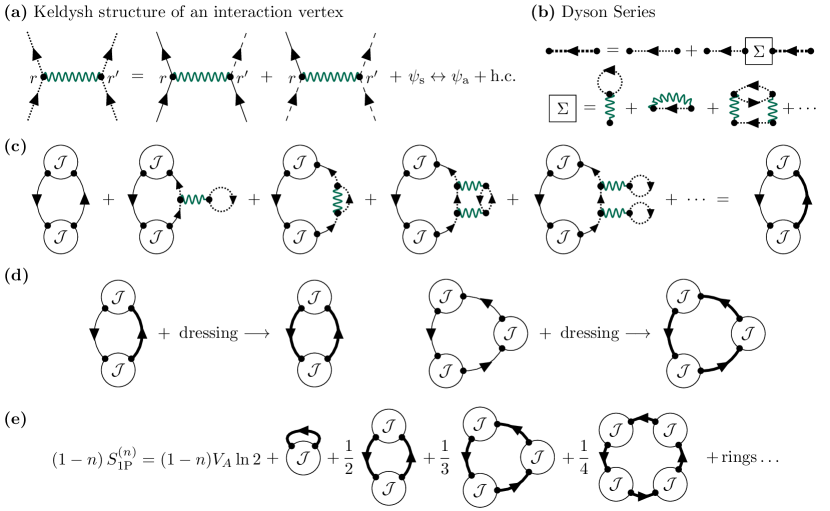
Figure 4: (a) Interaction vertices in Keldysh field theory corresponding to a pair wise interaction $\bar{\psi}_{r}\bar{\psi}_{r^{\prime}}U(r,r^{\prime})\psi_{r^{\prime}}\psi_{r}$. There are eight vertices in the $\psi_{\mathrm{s,a}}$ basis, each with an odd number of symmetric and antisymmetric fields, and a vertex factor of $\iota U(r,r^{\prime})/2$ (represented as a green wavy line). We use fields with dotted lines as a placeholder for both symmetric(solid) and antisymmetric(dashed) fields for the sake of brevity.(b) The presence of interactions induce self energy corrections $\Sigma$ which in turn dress the propagators. We use thick solid lines to signify the interacting Keldysh propagators. (c) & (d) Interaction dressing converts the free propagators in the ring diagrams to their interacting counterparts. (e) The one-particle contribution to $S^{(n)}$, $S^{(n)}_{1\mathrm{P}}$ is entirely determined by the sum of ring diagrams with the interacting Keldysh propagators.

III.1 One-particle correlators and $S^{(n)}_{1\mathrm{P}}$

We will first focus on calculating $S^{(n)}_{1\mathrm{P}}$. To do this, let us first consider the REE of a system of free fermions, where $S^{(n)}_{m\mathrm{P}}=0$ for $m>1$, i.e. $S^{(n)}=S^{(n)}_{1\mathrm{P}}$. For the diagrammatic expansion, we denote the symmetric fermionic fields by a solid line, and the anti-symmetric fields by dashed lines, as shown in Fig. 3(a). We have omitted spin indices, but they can be easily added to this description. Each field carries a replica index along with usual space-time indices. We will expand the free energy around the theory with $n$ independent identical replicas and treat $\mathcal{S}_{{\text{ent}}}$ as an additional coupling. In the independent replica theory, the propagators connect fields with same replica indices. The propagators for each replica are exactly the same as that of a single replica ( aka standard) Keldysh field theory. There are three independent propagators, the retarded propagator $G^{R}=-\iota\expectationvalue*{\psi_{\text{s}}\bar{\psi}_{\text{a}}}$, the advanced propagator $G^{A}=-\iota\expectationvalue*{\psi_{\text{a}}\bar{\psi}_{\text{s}}}$, and the Keldysh propagator $G^{K}=-\iota\expectationvalue*{\psi_{\text{s}}\bar{\psi}_{\text{s}}}$, as shown in Fig 3(b). Note $\expectationvalue*{\psi_{\text{a}}\bar{\psi}_{\text{a}}}=0$ in the single replica Keldysh field theory. These definitions hold for both the interacting and non-interacting theories. The quadratic coupling in $\mathcal{S}_{{\text{ent}}}$ is represented by an open circle, with the ${\cal J}$ vertex given by the matrix $\mathbb{J}\otimes\hat{P}_{A}$ as shown in Fig 3(c). Note that this vertex couples symmetric fields in different replicas on the same site in subsystem $A$ at the time when REE is computed.

The first point to note is that since the Rényi entropy is a free energy (in presence of inter-replica currents), it can be written as a sum of all fully connected diagrams in the replica field theory with no external legs. The second point to note is that the Keldysh free energy of the independent replicas is $0$, so the diagrams which contribute to REE must have one or more $\mathcal{S}_{{\text{ent}}}$ vertices. Finally, since $\mathcal{S}_{{\text{ent}}}$ is quadratic, one can easily re-sum all the diagrams here. Since the diagonal elements of $\mathbb{J}$ are $0$, there are no diagrams with a single ${\cal J}$ vertex. The first non-trivial diagram, which has two ${\cal J}$ vertices is shown in Fig. 3(d), together with its explicit evaluation. In fact, the set of ring diagrams shown in Fig. 3(e) exhausts all the free energy diagrams for the free theory. Note that only the Keldysh propagator, which carries information about distribution functions appear in this series. We note that the diagram with $p$ circles have a symmetry factor of $1/p$ ( $1/p!$ from the exponential and $(p-1)!$ from permutation of the $\cal J$ vertices). Defining $\iota\hat{G}^{K}_{0;A}=\hat{P}_{A}\iota\hat{G}^{K}(t_{o},t_{o})\hat{P}_{A}$ as the projection of the equal time Keldysh correlator onto the subsystem $A$, it is easy to see that

$$(1-n)S^{(n)}_{0} =(1-n)V_{A}\ln 2-\sum_{p=1}^{\infty}\frac{1}{p}\Tr_{\cal R}[{\mathbb{J}}^{p}]\Tr_{A}[(\iota\hat{G}_{0;A}^{K})^{p}]$$

$$=\ln(\frac{1}{2^{(n-1)V_{A}}}\det[\mathbb{I}\otimes\hat{1}-\mathbb{J}\otimes\iota\hat{G}^{K}_{0;A}]),$$ (18)

where $\mathbb{I}$ is the $n\times n$ identity matrix and $\hat{1}$ is the identitty operator on the subsystem $A$. This determinant is known exactly (see Appendix B of Ref. [38]), and it reduces to a closed form expression for $S^{(n)}_{0}$,

$$S^{(n)}_{0}(t_{o})=\frac{1}{1-n}\Tr_{A}\ln\left[(\hat{C}_{0}(t_{o}))^{n}+(\hat{1}-\hat{C}_{0}(t_{o}))^{n}\right],$$ (19)

where $C_{0}(i,j;t_{o})\equiv\expectationvalue*{\hat{c}^{\dagger}_{i}(t_{o})\hat{c}^{\vphantom{\dagger}}_{j}(t_{o})}_{0}$ is the non-interacting correlation matrix restricted to $A$, and is related to the equal-time Keldysh correlator by $\hat{C}_{0}(t_{o})=(\hat{1}-\iota\hat{G}^{K}_{0,A})/2$. Here $\hat{c}^{\dagger}_{i}$ creates a Fermion on site $i$. Eq. (19) matches with formulae derived earlier for non-interacting fermionic systems  [59, 60, 38]. This formula for REE of free fermions in terms of the one-particle correlation function is well known in the literature, and this acts as a check on our new method to calculate entanglement.

Let us now turn our focus to interacting Fermionic systems, where, for the sake of convenience, we assume a pairwise interaction,

$$\mathcal{S}_{{\text{int}}}^{\pm}=\pm\!\int\!\!\differential{t}\sum_{r,r^{\prime}}\bar{\psi}_{\pm}(r,t)\bar{\psi}_{\pm}(r^{\prime},t)\,U(r,r^{\prime})\psi_{\pm}(r^{\prime},t)\psi_{\pm}(r,t).$$

Here $r,r^{\prime}$ run over degrees of freedom in the whole system. We note that the final formulae we derive is agnostic to the precise form of the interaction; however assuming a representative form of $\mathcal{S}_{{\text{ent}}}$ helps us draw Feynman diagrams and clearly illustrate some of the properties of the formalism. In Sec. III.4, we outline a derivation of the same formulae without making reference to any particular form of interaction. For such a pairwise form the typical interaction vertices, shown in Fig 4(a), consist of three symmetric and one antisymmetric fields, or vice versa. Note that interaction vertex couples fields with the same replica index. It is still true that the Keldysh free energy of $n$ independent interacting replicas is $0$, so we only need to worry about connected diagrams with one or more open $\cal J$ vertices. It is instructive to think about the modifications of the ring diagrams due to interaction vertices. There is a set of diagrams where the interaction vertices couple fields on the same propagator. Some representative diagrams are shown on Fig. 4(c). These are essentially self-energy corrections to the propagators, shown in Fig. 4(b). The net effect of summing up all such diagrams is to convert the non-interacting one-particle correlator $\hat{C}_{0}$ to the interacting one particle correlator $\hat{C}$ in the expressions given in Eq. (19), as seen in Fig. 4(c) and Fig. 4(d). These dressed diagrams, depicted in Fig. 4(e), exhaust $S^{(n)}_{1\mathrm{P}}$ and other possible diagrams for $S^{(n)}$ depend on higher particle correlators. So, for interacting Fermions, we have

$$S^{(n)}_{1\mathrm{P}} =\frac{1}{1-n}\Tr_{A}\ln\left[\hat{C}^{n}+(\hat{1}-\hat{C})^{n}\right].$$ (20)

This is the analytic form of $S^{(n)}_{1\mathrm{P}}$ in terms of the exact interacting one-particle correlator (two-point function).

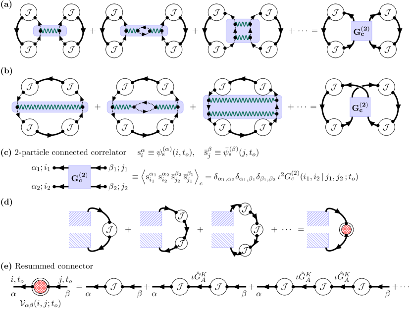
Figure 5: Feynman diagrams for the two-particle contribution to REE: (a) Propagators in two separate rings are connected by interaction vertices. Dressing of this pair of propagators converts them to an interacting connected two-particle correlator $G^{(2)}_{c}$ (shown in (c)). The rings are now connected and lead to a valid connected diagram for $S^{(n)}_{2\mathrm{P}}$. (b) A pair of propagator within the same ring is connected by interaction vertices and gets dressed to $G^{(2)}_{c}$. (a) and (b) can be viewed as diagrams where external legs of $G^{(2)}_{c}$ are connected by chains of entangling vertices ${\cal J}$ interlinked with single-particle propagators. (c) Details of the two particle connected correlator $G^{(2)}_{c}$. Note that it is diagonal in replica space. (d) Chains with different numbers of entangling vertices can be resummed into a single connector ${\cal\hat{V}}$. (e) The series for constructing ${\cal\hat{V}}$. The solid lines are interacting Keldysh propagators in a single replica. Detailed expressions for ${\cal\hat{V}}$ are provided in Eq. (22) and Eq. (23)

III.2 Two-particle correlators and $S^{(n)}_{\mathrm{2\mathrm{P}}}$

In a non-interacting system the one particle correlators define the density matrix and hence the REE [60]. However this is no longer true for interacting systems, where multi-particle connected correlators also contribute to the REE. To see this, let us focus on the first diagram shown in Fig. 5(a). Here we consider two otherwise disconnected rings, where an interaction line connects a propagator in one ring to a propagator in the other ring. This is now a connected diagram which contributes to $S^{(n)}$, but does not belong to the series of ring diagrams in $S^{(n)}_{1\mathrm{P}}$. The set of diagrams in Fig. 5 (a) shows how one can add more complicated motifs between the pair of propagators to convert them to the fully interacting connected two particle propagator (shaded region)

$$\iota^{2}G^{(2)}_{c}(i,j|k,l;t_{o}) =\expectationvalue{\psi_{\text{s}}(i,t_{o})\psi_{\text{s}}(j,t_{o})\bar{\psi}_{\text{s}}(l,t_{o})\bar{\psi}_{\text{s}}(k,t_{o})}_{c}$$

$$=2^{2}\expectationvalue{\hat{c}^{\dagger}_{k}\hat{c}^{\dagger}_{l}\hat{c}^{\vphantom{\dagger}}_{j}\hat{c}^{\vphantom{\dagger}}_{i}}_{c}.$$

An equivalent way of getting this diagram is to first consider the connected correlator $G^{(2)}_{c}$ and join its external legs through ${\cal J}$ vertices with interacting one particle propagators in between them. Note that each chain connecting the ends of $G^{(2)}_{c}$ should have at least one ${\cal J}$ vertex. Otherwise the two particle connected correlator would effectively reduce to a single particle propagator and reproduce diagrams in $S^{(n)}_{1P}$. It is simple to generalize to the case of $p$ rings where pair of propagators from the different rings are connected by interaction lines, leading to diagrams with multiple $G^{2}_{c}$. A second class of diagrams contributing to $S^{(n)}_{2P}$ can be obtained by considering pairs of propagators in a single ring and connecting them by interaction lines, effectively converting this pair to a $G^{(2)}_{c}$. A series of connections leading to such a diagram is shown in Fig. 5(b). In both cases (a) and (b), the resultant diagram can be reproduced by first considering $G^{(2)}_{c}$ and connecting its legs by chains of ${\cal J}$ vertices coupled by one particle propagators.

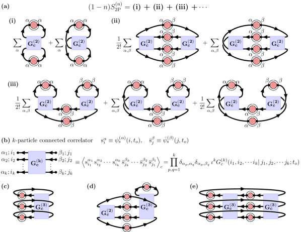
Figure 6: (a) The diagrams for $S^{(n)}_{2\mathrm{P}}$, which involve $1$ and $2$ $G^{(2)}_{c}$ s. (i),(ii),(iii) The diagrams shown exhaust all topologically distinct possibilities up to two instances of $G^{(2)}_{c}$. $\alpha,\beta$ are replica indices, and lattice indices are implied to be traced over the subsystem $A$. (b) The details of a $k$-particle connected correlator including replica and site indices. Note that all incoming and outgoing lines represent symmetric fields and carry the same replica index. (c)-(e) Some representative diagrams contributing to $S^{(n)}_{3\mathrm{P}}$. (c) involves a single $G^{(3)}_{c}$, (d) involves a $G^{(3)}_{c}$ and a $G^{(2)}_{c}$, while (e) involves two $G^{(3)}_{c}$s.

At this point, it is useful to note that each chain connecting the external legs of $G^{(2)}_{c}$ can have $1$, $2$, $3$, any number of ${\cal J}$ vertices. This is depicted in Fig. 5(d). One can then use a resummed one-particle connector ${\cal\hat{V}}$ to join the external legs of $G^{(2)}_{c}$ (see Sec. III.4 for details). The diagrammatic series corresponding to this resummation is shown in Fig. 5(e), which evaluates to the following for $\cal\hat{V}$,

$$\mathcal{\hat{V}}_{\alpha\beta} =\sum_{p=1}^{\infty}\left[{\,\mathbb{J}^{p}\,}\right]_{\alpha\beta}\,\left[\iota\hat{G}_{A}^{K}(t_{o},t_{o})\right]^{p-1},$$

$$=\left[{\,\mathbb{J}\otimes\hat{1}\left(\mathbb{I}\otimes\hat{1}-\mathbb{J}\otimes\iota\hat{G}^{K}_{A}\right)^{-1}}\right]_{\alpha\beta},$$ (21)

where $\iota\hat{G}^{K}_{A}=\hat{P}_{A}\hat{G}^{K}(t_{o},t_{o})\hat{P}_{A}$ is the interacting one particle Keldysh correlator at equal times, restricted to the subsystem $A$. It is possible to analytically obtain an expression for the matrix elements of $\cal\hat{V}$, namely,

$$[\mathcal{\hat{V}}_{\alpha\beta}]=\begin{bmatrix}\hat{v}_{0}&-\hat{v}_{n-1}&-\hat{v}_{n-2}&\cdots&-\hat{v}_{1}\\ \hat{v}_{1}&\hat{v}_{0}&\ddots&\ddots&\vdots\\ \hat{v}_{2}&\ddots&\ddots&\ddots&-\hat{v}_{n-2}\\ \vdots&\ddots&\ddots&\hat{v}_{0}&-\hat{v}_{n-1}\\ \hat{v}_{n-1}&\cdots&\hat{v}_{2}&\hat{v}_{1}&\hat{v}_{0}\end{bmatrix},$$ (22)

where

$$\hat{v}_{0} =\frac{1}{2}\frac{\hat{C}^{n-1}-(\hat{1}-\hat{C})^{n-1}}{\hat{C}^{n}+(\hat{1}-\hat{C})^{n}},$$ (23)

$$\hat{v}_{k} =\frac{1}{2}\frac{\hat{C}^{n-k-1}(\hat{1}-\hat{C})^{k-1}}{\hat{C}^{n}+(\hat{1}-\hat{C})^{n}}{\text{ for }}1\leq k\leq n-1.$$

This resummed connector is denoted diagrammatically by two concentric open circles with the inner one filled in with a cross-hatch pattern. Note that while the $\mathcal{J}(=\mathbb{J}\otimes\hat{P}_{A})$ vertex had only off-diagonal components in replica space, $\mathcal{\hat{V}}$ can couple fields with same replica indices as well. In this new language, we consider the interacting two-particle connected correlator and join its external legs by the $\mathcal{\hat{V}}$ connectors to rewrite the diagrams of Fig. 5(a) and (b). These are shown in Fig. 6(a-i).

Now, one can construct a larger class of diagrams which only involve the fully interacting $G^{(2)}_{c}$ and $\mathcal{\hat{V}}$s. To construct these diagrams consider $p$ different $G^{(2)}_{c}$ s, and connect their external legs by $\mathcal{\hat{V}}$s, so that no external leg remains unconnected. One can show (see Sec. III.4) that the symmetry factor of the diagram is simply determined by considering the possible permutations of the $G^{(2)}_{c}$ blocks. All the diagrams involving one or two $G^{(2)}_{c}$ blocks are shown in Fig. 6(a). The sum of all such diagrams which depend only on the 1-particle and 2-particle correlators, with the number of the latter varying from $1$ through $\infty$, forms $S^{(n)}_{2\mathrm{P}}$. This can be neatly summarized in the Feynman rules for diagrams in $S^{(n)}_{2\mathrm{P}}$:

• Consider $p$ two particle connected correlators and join their external legs in all topologically distinct ways.

• For each connected correlator, put a factor of $\iota^{2}G^{(2)}_{c}(i,j|k,l;t_{o})$, for each line joining external legs, put a factor of the resummed connector ${\cal\hat{V}}_{\alpha\beta}(i,j;t_{o})$.

• Sum over possible replica indices (noting that external legs of $G^{(2)}_{c}$ belong to the same replica).

• Sum over site indices in the subsystem $A$.

• Multiply by $(-1)^{N_{L}}$, where $N_{L}$ is the number of Fermion loops.

• Multiply each diagram by its symmetry factor (see Sec. III.4 for details)

Using these Feynman rules one can see that the first diagram in Fig 6(a-i) evaluates to

$$-n\sum_{ijkl\in A}G^{(2)}_{c}(i,j|k,l;t_{o})\,v_{0}(k,i;t_{o})\,v_{0}(l,j;t_{o}).$$ (24)

Similarly the first diagram (of ladder topology) shown in Fig. 6(a-ii) is given by

$$\hphantom{-}\frac{1}{2}\sum_{\alpha\beta}\sum_{\begin{subarray}{c}ijkl\\ xyzw\end{subarray}\in A}G^{(2)}_{c}(i,j|k,l)\,G^{(2)}_{c}(x,y|z,w)\,{\cal V}_{\alpha\beta}(k,x)\,{\cal V}_{\alpha\beta}(l,y)\,{\cal V}_{\beta\alpha}(z,i)\,{\cal V}_{\beta\alpha}(w,j),$$ (25)

while the first diagram (of bubble topology) in Fig. 6(a-iii) evaluates to

$$-\frac{1}{2}\sum_{\alpha\beta}\sum_{\begin{subarray}{c}ijkl\\ xyzw\end{subarray}\in A}G^{(2)}_{c}(i,j|k,l)\,G^{(2)}_{c}(x,y|z,w)\,{\cal V}_{\alpha\alpha}(k,i)\,{\cal V}_{\beta\beta}(z,x)\,{\cal V}_{\alpha\beta}(l,y)\,{\cal V}_{\beta\alpha}(w,j).$$ (26)

We have suppressed the time index in the above two equations for the sake of clarity. Summing over all such diagrams yields $S^{(n)}_{2\mathrm{P}}$. We thus have a prescription for construction of $S^{(n)}_{2P}$ from the one-particle and two-particle correlators.

III.3 $m$-particle correlators and $S^{(n)}_{m\mathrm{P}}$

Once we have established the Feynman rules for constructing the two-particle contribution to REE, $S^{(n)}_{2\mathrm{P}}$, it is easy to extend it to the case of $S^{(n)}_{m\mathrm{P}}$. Note that by definition, diagrams for $S^{(n)}_{m\mathrm{P}}$ must have at least one instance of the $m$-particle connected correlator

$$\iota^{m}\,G^{(m)}_{c}(i_{1},i_{2},\cdots i_{m}|j_{1},j_{2},\cdots j_{m};t_{o})$$ (27)

$$\hskip 5.0pt=\expectationvalue{\psi_{\text{s}}(i_{1},t_{o})\cdots\psi_{\text{s}}(i_{m},t_{o})\bar{\psi}_{\text{s}}(j_{m},t_{o})\cdots\bar{\psi}_{\text{s}}(j_{1},t_{o})}_{c}$$

$$\hskip 5.0pt=(-2)^{m}\expectationvalue{\hat{c}^{\dagger}_{j_{m}}\cdots\hat{c}^{\dagger}_{j_{2}}\hat{c}^{\dagger}_{j_{1}}\hat{c}^{\vphantom{\dagger}}_{i_{1}}\hat{c}^{\vphantom{\dagger}}_{i_{2}}\cdots\hat{c}^{\vphantom{\dagger}}_{i_{m}}}_{c}.$$

The diagrams cannot contain higher order ($k>m$) correlators. Now, $G^{(m)}_{c}$ has $m$ incoming lines and $m$ outgoing lines. Each of these outgoing lines can be (a) connected to the incoming lines of same $G^{(m)}_{c}$. Fig. 6(c) shows such a diagram for $G^{(3)}_{c}$. (b) connected to incoming lines of some other $G^{(k)}_{c}$ with $k<m$. Fig. 6(d) shows such a diagram where some of the outgoing lines of $G^{(3)}_{c}$ are connected to the incoming lines of a $G^{(2)}_{c}$. (c) connected to incoming lines of another $G^{(m)}_{c}$. Fig. 6(e) shows such a diagram where two $G^{(3)}_{c}$ s are connected to each other. We draw topologically distinct connected diagrams where all the incoming and outgoing lines are joined with $\cal\hat{V}$ vertices, making it a free energy diagram. The symmetry factor is determined by considering permutations of the connected correlators in the usual way. The sum of all such diagrams give $S^{(n)}_{m\mathrm{P}}$. The Feynman rules for these diagrams are simple extensions of those for $S^{(n)}_{2\mathrm{P}}$:

• Consider at least one $m$-particle connected correlator and any number of $k$-particle connected correlators with $k<m$. Join their external legs in all topologically distinct ways, so that no external lines remain hanging.

• Draw only fully connected diagrams.

• For each $k$-particle connected correlator, put a factor of $\iota^{k}G^{(k)}_{c}(i_{1},..i_{k}|j_{1},..j_{k};t_{o})$, for each line joining external legs, put a factor of the resummed connector ${\cal\hat{V}}_{\alpha\beta}(i,j;t_{o})$.

• Sum over possible replica indices (noting that external legs of $G^{(k)}_{c}$ belong to the same replica).

• Sum over site indices in the subsystem $A$.

• multiply by $(-1)^{N_{L}}$, where $N_{L}$ is the number of Fermion loops.

• Multiply each diagram by its symmetry factor (see Sec. III.4 for details).

This provides a general prescription to construct the $m$-particle contribution to the Rényi entropy $S^{(n)}_{m\mathrm{P}}$. Some representative diagrams in the construction of $S^{(n)}_{3\mathrm{P}}$, which involve $G^{(2)}_{c}$ and $G^{(3)}_{c}$ are shown in Fig. 6(b-d). As an instance of employing the Feynman rules, the diagram in Fig. 6(b) is given by (time index suppressed)

$$n\sum_{\begin{subarray}{c}i,j,k\\ x,y,z\end{subarray}\in A}\iota^{3}G^{(3)}_{c}(i,j,k|x,y,z)\,v_{0}(x,i)\,v_{0}(y,j)\,v_{0}(z,k).$$ (28)

One can now use the Feynman rules given above to construct diagrams and convert them into integral contributions to $S^{(n)}_{m\mathrm{P}}$. We note here for completeness that diagrams constructed following the aforementioned rules will contribute to $(1-n)S^{(n)}_{m\mathrm{P}}$. We have thus provided a general prescription of constructing an estimate of Rényi entanglement entropy if we only have knowledge of upto $m$-particle connected correlation functions.

III.4 General Derivation

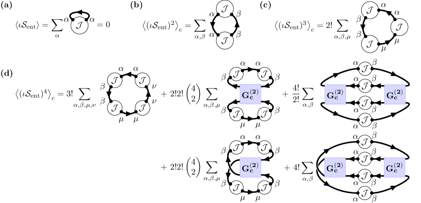
Figure 7: Feynman diagrams from cumulant expansion: (a)-(c) Diagrams corresponding to the first three cumulants of $\iota\mathcal{S}_{{\text{ent}}}$. Replica indices are explicitly marked on each propagator whereas lattice indices are implied to be traced over. (d) Diagrams corresponding to the fourth cumulant of $\iota\mathcal{S}_{{\text{ent}}}$. Note that this involves diagrams which form part of $S^{(n)}_{1\mathrm{P}}$ (first diagram) as well as diagrams which form part of $S^{(n)}_{2\mathrm{P}}$ (last 4 diagrams). Similarly the sixth cumulant will have terms belonging to $S^{(n)}_{3\mathrm{P}}$ as well as $S^{(n)}_{1\mathrm{P}}$ and $S^{(n)}_{2\mathrm{P}}$. Note that each of $S^{(n)}_{m\mathrm{P}}$ has contribution from an infinite set of cumulants starting at order $2m$. The cumulants simply correspond to a different grouping of all the diagrams discussed earlier.

In the discussion so far, we started by inspecting what effect a “replica current” term $\mathcal{S}_{{\text{ent}}}$ would have on the free energy diagrams of $n$ independent free theories $\mathcal{S}_{0}$. We then proceeded to add interactions $\mathcal{S}_{{\text{int}}}$ in each replica to argue for, and illustrate, various non-perturbative effects. In this section we instead choose to formally expand Eq. (13) in cumulants of $\iota\mathcal{S}_{\text{ent}}$ and evaluate them in terms of connected correlators in the (un-replicated) interacting theory $\mathcal{S}_{0}+\mathcal{S}_{{\text{int}}}$. This will provide a first principles derivation of the previously stated results which makes no appeal to the form or nature of $\mathcal{S}_{{\text{int}}}$.

We crucially use three facts mentioned earlier, but reiterated here for emphasis: (i) REE $S^{(n)}$ is equivalent to a Keldysh free energy of $n$ independent replicas in presence of the entangling action $\mathcal{S}_{{\text{ent}}}$ (ii) Keldysh partition functions are inherently normalised to unity in the absence of sources which implies that all diagrams must include at least one instance of $\mathcal{S}_{{\text{ent}}}$ (iii) All correlators which occur in the diagrammatic expansion are “standard” Schwinger-Keldysh correlators of a single replica; i.e. these are the correlation functions one finds in standard textbooks [69]. Owing to the structure of $\mathcal{S}_{{\text{ent}}}$, only equal time correlators of the symmetric fields, restricted to the subsystem $A$, will make an appearance. With this in mind, $\Tr[\hat{\rho}_{A}^{n}]$ can be viewed as an expectation value of $\,\mathrm{e}^{\iota\mathcal{S}_{\text{ent}}}$ in $n$ independent copies of the interacting theory,

$$\,\mathrm{e}^{-(n-1)(S^{(n)}-V_{A}\ln 2)}=\expectationvalue{\,\mathrm{e}^{\iota{\cal S}_{\text{ent}}}}_{n},$$

where the subscript on $\expectationvalue{\bullet}_{n}$ denotes the number of independent copies of the action $\mathcal{S}_{K}$. The REE $S^{(n)}$ can be obtained as the cumulant expansion of the above,

$$(1-n)(S^{(n)}-V_{A}\ln 2)$$

$$\hphantom{-}=\expectationvalue{\iota\mathcal{S}_{\text{ent}}}+\frac{1}{2!}\expectationvalue{(\iota\mathcal{S}_{\text{ent}})^{2}}_{c}+\frac{1}{3!}\expectationvalue{(\iota\mathcal{S}_{\text{ent}})^{3}}_{c}+\cdots,$$ (29)

where $\expectationvalue{\bullet}_{c}$ represents the connected part of the expectation value calculated with respect to the $n$ independent replicas.For example, in case of the second cumulant $\expectationvalue{(\iota\mathcal{S}_{\text{ent}})^{2}}_{c}=\expectationvalue{(\iota\mathcal{S}_{\text{ent}})^{2}}_{n}-\expectationvalue{\iota\mathcal{S}_{\text{ent}}}^{2}_{n}$ . We will employ the diagrammatic rules set up previously to evaluate these cumulants. A $p$^th order cumulant will involve all possible topologically distinct connected diagrams made out of $p$ number of $\mathcal{J}$ vertices. The first few orders are depicted in Fig. 7. Since the $\cal J$ vertex doesn’t connect fields in the same replica, the first cumulant $\expectationvalue{\iota\mathcal{S}_{{\text{ent}}}}_{n}$ is exactly zero. This simplifies the diagrams at higher orders. In particular, till the third cumulant, the only possible fully connected diagrams are ring diagrams as shown in Fig. 7(a)-(c). Explicitly evaluating the diagram in Fig. 7(b) and (c) we get,

$$\expectationvalue{(\iota\mathcal{S}_{{\text{ent}}})^{2}}_{c} =-\Tr_{\cal R}[\mathbb{J}^{2}]\Tr_{A}[(\iota\hat{G}^{K}_{A})^{2}],$$

$$\expectationvalue{(\iota\mathcal{S}_{{\text{ent}}})^{3}}_{c} =-2!\Tr_{\cal R}[\mathbb{J}^{3}]\Tr_{A}[(\iota\hat{G}^{K}_{A})^{3}].$$

where $\iota\hat{G}^{K}_{A}=\hat{P}_{A}\iota\hat{G}^{K}(t_{o},t_{o})\hat{P}_{A}$ is the equal time two-point Keldysh correlator evaluated in the interacting theory and restricted to subsystem $A$. In a similar fashion, every higher order cumulant will give rise to a ring diagram of $\mathcal{J}$ vertices, with the number of cyclic permutations at order $p$ being $(p-1)!$. Taken together with the combinatorial factor of $1/p!$ in the definition of the cumulant expansion, the weight of a ring diagram at order $p$ is $1/p$. Grouping all order ring diagrams together we have recovered the $1$-particle contribution to $S^{(n)}$, $S^{(n)}_{1\mathrm{P}}$ as depicted in Fig. 4(e), and consequently the analytic form of the same in terms of the interacting correlation function $C$ in Eq. (20).

In higher order cumulants, connected diagrams of $\cal J$ vertices can also be constructed using multiparticle connected correlators. For example Fig. 7(d) shows the diagrams with $G^{(2)}_{c}$ that contribute to the fourth order cumulant. In fact, the $p$^th order cumulant will involve all possible fully connected diagrams with $p$ instances of the entangling vertex $\mathcal{J}$ joined by all possible $k$-particle equal time connected Keldysh correlators $G^{(k)}_{c}$ with $2k\leq p$.

We now turn to classifying the diagrams based on their correlator content. Diagrams with atleast one instance of the 2 body connected correlator $G^{(2)}_{c}$, but no higher body correlators are clubbed together as the “$2$-particle contribution”, $S^{(n)}_{2\mathrm{P}}$. Similarly we define the “$m$-particle contribution” to $S^{(n)}$ as the collection of all diagrams which contain atleast one instance of $G^{(m)}_{c}$ but none of the higher body correlators. This formal regrouping lets us write a “$m$-particle”-decomposition for EE as stated in Eq. (17). Given the structure of $S^{(n)}_{m\mathrm{P}}$, if the $m$^th correlator is factorisable, the entire collection of diagrams get decimated.

Each of these $m$-particle contributions contain a multitude of diagrams with different correlator content (number and type of $G^{(m)}_{c}$ boxes) and topologies. They also include infinitely many diagrams of the same topology and correlator content but with a variable number of $\cal J$ vertices on the lines between the $G^{(m)}_{c}$ boxes. Such diagrams can be clubbed together to get a resummed connector $\cal V$ on each line since the relative weights of the diagrams turn out to be exactly one. Assume a diagram of a given structure with a total of $p$ number of $\cal J$ vertices, distributed across $q$ different lines with the number in each line being $n_{1},n_{2},\cdots,n_{q}$. The ways of distributing $p$ identical vertices into $q$ lines with the number of vertices in each line fixed, gets exactly cancelled by the $1/p!$ from the cumulant expansion and $n_{j}!$ permutations from the $j$^th line,

$${\text{Weight}}=\frac{1}{p!}\times\frac{p!}{n_{1}!\,n_{2}!\,\cdots n_{q}!}\times(n_{1}!\,n_{2}!\,\cdots n_{q}!)=1.$$

This fact reproduces the series depicted in Fig. 5(d) and the functional forms in Eq. (23). This also makes it apparent that any and all symmetry factors for the diagram is determined from exchange of the correlator blocks. In summary, all diagrams are constructed following the Feynman rules laid down in the previous sections.

We have thus provided a constructive prescription for evaluating $S^{(n)}_{m\mathrm{P}}$ in a manner independent of the underlying theory of the problem. We note that if one is interested in the exact answer for entanglement, one has to compute upto $S^{(n)}_{V_{A}\mathrm{P}}$ and the complexity of the problem is same as exact diagonalization. However field theoretic methods are rarely good for exact answers, they are usually geared to provide useful approximate answers to various quantities. In this case, the decomposition of $S^{(n)}$ into $S^{(n)}_{m\mathrm{P}}$ is useful when the series can be truncated after a few terms to yield good estimates of entanglement. This will happen if the higher order connected correlators are parametrically small, i.e. the system is connected to a Gaussian theory by small couplings. This can happen in a weakly interacting Fermi liquid, where the higher order correlators occur at higher orders in the interaction strength. It can also happen if the Gaussian theory represents a symmetry broken mean field state, e.g. in a large $N$ theory of a superconductor or magnets, where higher order connected correlators have larger powers of $1/N$. In general, if one only has information about few body correlators, one can use this decomposition to obtain estimates of REE. The question of specific approximation schemes for particular situations is not discussed here. It will be taken up in future works.

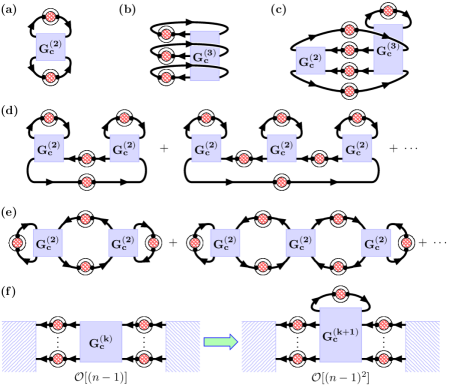
Figure 8: Examples of diagrams which do not contribute to EE, i.e. do not survive under analytic continuation $n\to 1$. (a)-(b) Diagrams with a single multi-particle correlator with external legs connected amongst themselves through $\hat{v}_{0}$. (a) scales like $\sim(n-1)^{2}$ whereas (b) scales as $\sim(n-1)^{3}$. (c) Diagram with mixed correlators scaling as $\sim(n-1)^{2}$ despite having only one instance of $\hat{v}_{0}$ . (d)-(e) Series of diagrams with recurrent motifs which get decimated in the $n\to 1$ limit. In (d) each successive diagram with $p$ motifis scales as atleast $\order{(n-1)^{p}}$, whereas in (e) each successive diagram scales as atleast $\order{(n-1)^{2}}$. Note that the first diagram in both series are topologically equivalent. It is included twice to emphasize the series structure. (f) A given diagram can be modified to generate new diagrams by replacing a $k$-particle connected correlator by a $(k+1)$-particle correlator with a contracted pair of legs. The extended diagram preserves the replica structure of connectors as in the original but scales with one higher power of $n-1$ in the $n\to 1$ limit. Such extensions are “irrelevant” for the analytic continuation, in the sense that if the original diagram survived the $n\to 1$ limit, the extended diagram would not. The diagram in (c) is such an irrelevant extension of a diagram which has a nonzero analytic continuation, and hence has a zero contribution itself.

IV Analytic continuation and von-Neumann Entropy

In the previous section we have shown a way to construct the $n$^th order Rényi entropy in terms of the multi-particle correlators of an interacting Fermionic system. In this section we will discuss how this can be used to obtain a construction of the von Neumann entropy (EE) $S=\lim_{n\to 1}S^{(n)}$. The diagrammatic construction discussed so far is given for $(1-n)S^{(n)}$. Hence, only diagrams which scale as $\sim(n-1)$ will contribute to $S$ in this expansion; terms $\sim\order{(n-1)^{2}}$ will not survive the analytic continuation.

Let us first consider the one-particle contribution $S_{1\mathrm{P}}$. Taking the analytic continuation of Eq. (20), one can easily show that

$$S_{1\mathrm{P}}=-\Tr[\hat{C}\ln\hat{C}+(\hat{1}-\hat{C})\ln(\hat{1}-\hat{C})].$$ (30)

It is hard to formulate such a general expression for analytic continuation of $S^{(n)}_{m\mathrm{P}}$. This is primarily because of the fact that elements of the matrix $\mathcal{\hat{V}}_{\alpha\beta}$ have explicit $n$ dependence as well as dependence on $\alpha-\beta$. Thus the $n$ dependence of different diagrams, which involve summing over replica indices, have to be calculated individually for each diagram and a priori cannot be captured by a general formula. However, a large class of diagrams vanish when the analytic continuation is taken and the diagrammatic expansion for $S$ has many diagrams less than that for $S^{(n)}$. To see this, note that in the limit $n\to 1$,

$$\hat{v}_{0}\sim\frac{n-1}{2}\ln\left[\frac{\hat{C}}{1-\hat{C}}\right]+\order{(n-1)^{2}}.$$ (31)

This has the immediate consequence that any term involving more than one instance of $\hat{v}_{0}$ must scale at least as $\sim(n-1)^{2}$ and hence have vanishing contribution in the $n\to 1$ limit. These $\hat{v}_{0}$ connectors may connect the external legs on the same correlator, or the legs from different correlators with the same replica index. As an example, consider diagrams like those in Fig. 8(a) & (b), where the external legs of a single multi-particle correlator are joined by the resummed connector $\mathcal{\hat{V}}$. Such diagrams necessarily contain more than one factor of $\hat{v}_{0}$ and are decimated under analytic continuation. Similarly one can show that entire series of diagrams vanish under analytic continuation due to this criterion. We depict two examples of such series in Fig. 8(d) & (e) which have the topology of Harteee corrections and RPA diagrams of many body theory respectively.

The leading scaling of $\hat{v}_{0}$ in the $n\to 1$ limit can also be used to constrain possible diagrams which have non-zero contribution to EE. Given a legitimate diagram with a $k$-particle correlator, we can generate another equally legitimate diagram from it by replacing the chosen correlator with a $(k+1)$-particle one with a pair of external legs self-contracted through $\hat{v}_{0}$, as shown in Fig. 8(f). This procedure keeps the replica structure of the connectors in the original diagram intact. However the presence of the extra $\hat{v}_{0}$ in the extended diagram increases the leading $(n-1)$ scaling by one power as compared to the original. If the original diagram had a non-zero contribution to EE, the diagram born from such an “irrelevant” extension will not contribute to EE. As an example, the diagram in Fig. 8(c) is an irrelevant extension of the diagram in Fig. 6(a-ii) and doesn’t contribute in the $n\to 1$ limit for EE.

We now turn to focus on diagrams which do survive in the $n\to 1$ limit. As an example, consider the analytic continuation of the diagrams for $S^{(n)}_{2\mathrm{P}}$ shown in Fig. 6(a). The diagrams of Fig. 6(a-i) and (a-iii) vanish in the $n\to 1$ limit, while the first non-trivial diagram for $S_{2\mathrm{P}}$ is given by the analytic continuation of the diagram in Fig 6(a-ii). For the evaluation of this diagram, it is more convenient to work in the eigenbasis of the interacting correlation matrix $C(i,j)$ restricted to the subsystem $A$, defined as $\hat{C}\ket{c_{m}}=c_{m}\ket{c_{m}}$ where $c_{m}$ and $\ket{c_{m}}$ are respectively the eigenvalues and eigenvectors of $\hat{C}$. For $n\to 1$, this diagram gives (see Appendix B for details)

$$-\frac{1}{32}\sum_{c_{1},c_{2},c_{3},c_{4}}\frac{\ln(x)-\ln(y)}{x-y}\left|\matrixelement{c_{1},c_{2}}{\hat{G}^{(2)}_{c}}{c_{3},c_{4}}\right|^{2},$$ (32)

where $x=c_{1}c_{2}(1-c_{3})(1-c_{4})$ and $y=(1-c_{1})(1-c_{2})c_{3}c_{4}$, and $\ket{c_{1},c_{2}}=\ket{c_{1}}\otimes\ket{c_{2}}$. The arguments presented in Appendix B can be readily adapted to analytically continue other diagrams with the same replica connection structure, such as the diagram in Fig. 6(e).

So far we have assumed that the expression in Eq. (32) is finite. Indeed the $(\ln x-\ln y)/(x-y)$ factor in the summand of Eq. (32) is finite for $x=y$ but diverges when either of $x,y\to 0$. It is a priori unclear if the matrix elements of $G^{(2)}_{c}$ are sufficiently small in this regime to result in a finite answer for this diagram. In case they do not converge, the program of diagram-by-diagram analytic continuation falls under suspicion and some appropriate subset of diagrams in $S^{(n)}_{m\mathrm{P}}$ might have to be resummed first and then analytically continued. Such considerations and its implications for entanglement are left as topics of future work.

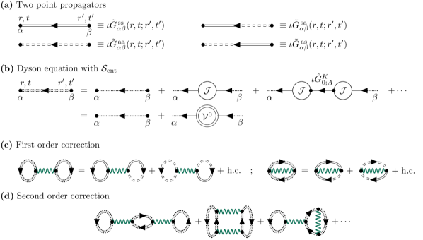
Figure 9: Feynman diagrams for Rényi entanglement entropy using propagators in the replicated theory. (a): Single particle propagators $\tilde{G}$ in the non-interacting theory with the replica coupling term $\mathcal{S}_{{\text{ent}}}$ included. We use double lines for these propagators and single lines for propagators in a single replica ($G$). $\alpha$ $\beta$ are the replica indices. Note that $\tilde{G}^{\rm\,aa}$ is finite in this theory, in contrast to a single replica Keldysh theory. (b): The Dyson series for the $\tilde{G}$ in terms of $G$ and the entanglement vertex ${\cal J}$. The structure of the Dyson equation is similar for all Keldysh components. Hence a single diagram with dotted lines is used to show this. The specific Keldysh components can easily be obtained from this by replacing the dotted external lines with a solid (symmetric) or a dashed (antisymmetric) line. Note that for $\tilde{G}^{\rm\,aa}$, the first term $\expectationvalue*{\psi_{\text{a}}\bar{\psi}_{\text{a}}}_{0}=0$. (c): Diagrams showing the first order correction due to interaction vertices. The diagrams are drawn with double dotted lines to show their structural similarity with standard free energy diagrams in equilibrium field theory (Direct and Exchange terms). However, the propagators here carry Keldysh indices and only particular combinations are allowed by interaction vertices. This is explicitly shown in (c) for the first order diagrams. Note that lines emanating from an interaction vertex must have the same replica index. (d): Feynman diagrams corresponding to second order corrections in the interaction strength. Only the structure of diagrams is shown with dotted lines for the sake of brevity.

V Beyond Standard Keldysh Field Theory

In section III.1, we have shown that the $n$^th Rényi entropy of a system of interacting Fermions is the Keldysh free energy of n replicas governed by an action, $\mathcal{S}_{0}+\mathcal{S}_{\text{int}}+\mathcal{S}_{{\text{ent}}}$, where $\mathcal{S}_{0}$ is the non-interacting (quadratic) action for decoupled replicas, $\mathcal{S}_{\text{int}}$ is the interacting part of the action for decoupled replicas and $\mathcal{S}_{{\text{ent}}}$ is the quadratic action which couples the different replicas and generates entanglement. In section III.4, we expanded the free energy around $\mathcal{S}_{0}+\mathcal{S}_{\text{int}}$ and connected entanglement entropy with interacting connected correlators in the usual single replica theory. However, one can also think of solving $\mathcal{S}_{0}+\mathcal{S}_{{\text{ent}}}$ exactly since this is still a quadratic action, and use the resulting propagators to expand in $\mathcal{S}_{\text{int}}$. Note that this is a regrouping of the terms worked out earlier. In this section we will work out this expansion and resultant diagrammatics.

The earlier expansion around $\mathcal{S}_{0}+\mathcal{S}_{\text{int}}$ had the advantage that it used propagators and correlators which can be related to observable correlations in the system. The one-particle propagators, for example, can be grouped into retarded, advanced or Keldysh propagators with well known properties and relations to measured quantities. The current expansion will work with propagators which are matrices in replica space and cannot be immediately related to observables. They will not follow the clear demarcation into retarded, advanced or Keldysh propagators, at least they will not inherit their well known properties. However, there are two advantages to the current expansion: (i) the organization of diagrams is simpler, since the replica space propagators already incorporate resummations due to $\mathcal{S}_{{\text{ent}}}$ and (ii) this expansion will tie up vertex functions rather than correlation functions. This can be of relevance if one is interested in calculating “effective entanglement actions” under various circumstances with the “effective entanglement action” playing a similar role as that of modular Hamiltonians [76] used to study entanglement entropy. Since this maintains the language of an effective action, this is also the natural language to introduce techniques like auxiliary fields, saddle points etc. This is also the natural language to think about renormalization group in this context.

Let us first focus on $\mathcal{S}_{0}+\mathcal{S}_{{\text{ent}}}$. In this case both the fields and the propagators carry space-time, Keldysh and replica indices (one can add spin or other quantum numbers as well). Using $\mathcal{S}_{{\text{ent}}}$ as a self energy correction, one can solve the Dyson series exactly (see Fig. 9(b)), and define the propagators

$$\tilde{G}^{\rm\,sa}_{\alpha\beta}(r,t;r^{\prime},t^{\prime}) =\delta_{\alpha\beta}G^{R}_{0}(r,t;r^{\prime},t^{\prime})+\iota\sum_{i,j\in A}G^{K}_{0}(r,t;i,t_{o})\,{\cal V}^{0}_{\alpha\beta}(i,j)\,G^{R}_{0}(j,t_{o};r^{\prime},t^{\prime}),$$ (33)

$$\tilde{G}^{\rm\,as}_{\alpha\beta}(r,t;r^{\prime},t^{\prime}) =\delta_{\alpha\beta}G^{A}_{0}(r,t;r^{\prime},t^{\prime})+\iota\,\sum_{i,j\in A}G^{A}_{0}(r,t;i,t_{o})\,{\cal V}^{0}_{\alpha\beta}(i,j)\,G^{K}_{0}(j,t_{o};r^{\prime},t^{\prime}),$$

$$\tilde{G}^{\rm\,ss}_{\alpha\beta}(r,t;r^{\prime},t^{\prime}) =\delta_{\alpha\beta}G^{K}_{0}(r,t;r^{\prime},t^{\prime})+\iota\,\sum_{i,j\in A}G^{K}_{0}(r,t;i,t_{o})\,{\cal V}^{0}_{\alpha\beta}(i,j)\,G^{K}_{0}(j,t_{o};r^{\prime},t^{\prime}),$$

$$\tilde{G}^{\rm\,aa}_{\alpha\beta}(r,t;r^{\prime},t^{\prime}) =\iota\,\sum_{i,j\in A}G^{A}_{0}(r,t;i,t_{o})\,{\cal V}^{0}_{\alpha\beta}(i,j)\,G^{R}_{0}(j,t_{o};r^{\prime},t^{\prime}),$$

where $G^{R}_{0}$, $G^{A}_{0}$ and $G^{K}_{0}$ are the retarded, advanced, and Keldysh propagators of the single replica Keldysh field theory without interactions. $\mathcal{\hat{V}}^{0}$ has the same structure as in Eq. (22) but with the non-interacting correlation matrix determining the blocks in Eq. (23). We denote this difference by using concentric empty circles to represent $\cal\hat{V}_{0}$ in contrast to the cross-hatched concentric circles used for $\cal\hat{V}$. These propagators and the Dyson series for them is shown in Fig. 9(a) and (b). Although these propagators are not directly related to observables, they can be constructed out of the standard one-particle propagators. We note that in this case $\tilde{G}^{\rm\,sa}$ is not a retarded propagator, nor is $\tilde{G}^{\rm\,as}$ an advanced propagator, although the relation $\left(\tilde{G}^{\rm\,as}\right)^{\dagger}=\tilde{G}^{\rm\,sa}$ still holds. Further, unlike the standard Keldysh theory, $\tilde{G}^{\rm\,aa}$ is non-zero due to the presence of $\mathcal{S}_{{\text{ent}}}$ in the action. It is easy to show that $G^{\rm\,ss}$ and $G^{\rm\,aa}$ are both anti-Hermitian in this replicated theory. These propagators are represented by a double line in the diagrams.

One can now work out the diagrammatic expansion of the free energy in terms of the original interaction vertices in $\mathcal{S}_{{\text{int}}}$ and the new propagators in the usual way:(a) draw all topologically distinct connected diagrams. (b) For each interaction vertex, put $\iota U(r,r^{\prime})/2$, where $U(r,r^{\prime})$ is the matrix element of the interaction, for each propagator put a factor of $\iota\tilde{G}$. (c) multiply by symmetry factor and $(-1)^{n_{L}}$, where $n_{L}$ is the number of Fermion loops (d) Sum over all internal indices (over all space and time, not only in the subsystem). Three important things need to be kept in mind: (i) The fields coming out of any interaction vertex belongs to the same replica, (ii) The propagators $\tilde{G}(r,t;r^{\prime},t^{\prime})$ are supported over the entire system and generically lack translational invariance due to the presence of the entanglement cut, and (iii) Certain diagrams which vanish in standard Keldysh field theory give finite contribution, as $\tilde{G}^{\rm\,aa}$ are finite in this theory. The first order correction to $S^{n}$ is shown in Fig. 9(c). The first of these diagrams (the direct contribution) evaluates to

$$\delta S^{(n)}=(-\iota)\,\sum_{\alpha}\,\int\differential{t}\sum_{r,r^{\prime}}\left[\tilde{G}^{\rm\,ss}_{\alpha\alpha}(r,t;r,t)+\tilde{G}^{\rm\,aa}_{\alpha\alpha}(r,t;r,t)\right]U(r,r^{\prime})\left[\tilde{G}^{\rm\,as}_{\alpha\alpha}(r^{\prime},t;r^{\prime},t)+\tilde{G}^{\rm\,sa}_{\alpha\alpha}(r^{\prime},t;r^{\prime},t)\right],$$ (34)

while the second diagram (the exchange contribution) is given by

$$\delta S^{(n)}=(\iota)\,\sum_{\alpha}\,\int\differential{t}\sum_{r,r^{\prime}}\left[\tilde{G}^{\rm\,ss}_{\alpha\alpha}(r,t;r^{\prime},t)+\tilde{G}^{\rm\,aa}_{\alpha\alpha}(r,t;r^{\prime},t)\right]U(r,r^{\prime})\left[\tilde{G}^{\rm\,as}_{\alpha\alpha}(r^{\prime},t;r,t)+\tilde{G}^{\rm\,sa}_{\alpha\alpha}(r^{\prime},t;r,t)\right].$$ (35)

One can similarly evaluate other diagrams, some of which are shown in Fig. 9(d). One can thus reconstruct the diagrammatic series in terms of the replica propagators and the original interaction vertices. We note that while the propagators cannot be related to anything physical, the number of diagrams reduce considerably in this way of grouping the terms. However, in absence of physical correlators, one needs to construct useful approximate truncations of the diagrams. While a perturbation theory immediately provides a truncation, one should be more careful about constructing non-perturbative approximations in this non-standard Keldysh field theory.

VI Conclusions

In this paper, we have formulated a new way of calculating entanglement entropy of a generic interacting Fermionic system from the knowledge of correlation functions in the subsystem. Using a Wigner function based method, coupled with Schwinger Keldysh field theory, we show that the $n$^th Rényi entropy $S^{(n)}$ is the Keldysh free energy of a theory of $n$ replicas which are coupled by inter-replica currents, which exist in the subsystem. These currents are local in space-time, i.e. they are turned on between same degrees of freedom at the time of measurement of the entanglement theory. These currents have a structure which is not allowed in usual Keldysh field theory with a single replica, and hence we do not have an equivalent formulation in usual single-contour field theories. These currents implement the boundary condition matching required in standard replica formulation of entanglement theory.

Starting from this description of EE as a free energy in presence of inter-replica currents, we show that the EE can be written as a sum of terms which require knowledge of progressively higher order connected correlators in the system. These correlators are usual field theoretic observables, calculated in a standard ffield theory with no replicas and correspond to measureables in the system. We provide an analytic formula for the single-particle contribution to entanglement; we also provide a diagrammatic construction for the contribution of higher particle correlators to EE. We thus relate the correlation functions in a system to its . These constructions are agnostic to how the correlators are calculated, and hence forms a universal basis for further approximate calculations. One can also use experimentally measured correlation functions in these formulae to calculate entanglement. They provide estimates for entanglement when only a few order correlation functions are known. This reduces the complexity of calculating entanglement entropies vis a vis direct methods which requires the knowledge of the full quantum many body state.

We have considered how one can implement the analytic continuation required to obtain the von-Neumann entropy $S$ from the Rényi entropy. We obtain analytic formula for the single-particle contribution to $S$ in terms of interacting one-particle distributions. We show that a large class of diagrams for multi-particle contributions vanish under the analytic continuation. We calculate an analytic formula for the first non-trivial diagram for two-particle contribution to $S$.

Technically we achieve this in two different ways,(a) by constructing an expansion around an interacting theory with independent replicas. This provides a relation between observables and entanglement and is useful for gaining insights. (b) by constructing an expansion around a non-interacting theory of coupled replicas. While this method is less insightful, it provides a simpler construction of diagrams, since large class of individual diagrams in the first method are re-summed into single objects in this case. While the first method provides relation between correlations and entanglement, the second method provides a relation between vertex functions and entanglement, and may be more suitable for treatments like renormalization group analysis.

We note that what we have done here is akin to setting up a general diagrammatic expansion and writing down the Feynman diagrams and Feynman rules for the calculation of entanglement entropy. Calculations for particular systems would require further approximations. One can ask the following question: In general correlations will be calculated using approximation methods. One would have to further truncate/approximate using a subset of the diagrams we have drawn here. For simple approximations like perturbation theory or large $N$ approximations, it is clear how such a truncation will happen. However for non-perturbative approximations, it may turn out that certain approximations for correlators are compatible with certain subsets of these diagrams. Is there a general rule for such compatibility? We do not take up this question in this work, but leave it as a general question to be answered in future works.

Appendix A Equal time Keldysh correlators in terms of operators

In this section we provide the explicit form of the many-particle equal time Keldysh correlators in terms of electron operators. These will be useful when connecting our formalism to numerical simulations or experiments measuring such correlators.

Like in usual quantum field theory, the Schwinger Keldysh partition function in presence of sources, $\mathcal{Z}[J_{\mathrm{s,a}},\bar{J}_{\mathrm{s,a}}]$ is the generating function of $k$-particle correlators, and $\ln\mathcal{Z}$ is the generating function for connected correlators. In particular, to get the $k$-particle Keldysh correlator involving all symmetric fields, we take derivatives of $\ln\mathcal{Z}$ w.r.to the antisymmetric sources,

$$\expectationvalue{\psi_{\mathrm{s}}(1)\cdots\psi_{\mathrm{s}}(k)\bar{\psi}_{\mathrm{s}}(k^{\prime})\cdots\bar{\psi}_{\mathrm{s}}(1^{\prime})}_{c}$$ (36)

$$=\left.\frac{\delta^{2k}\ln\mathcal{Z}[J_{\mathrm{a,s}},\bar{J}_{\mathrm{a,s}}]}{\delta\bar{J}_{\mathrm{a}}(1)\cdots\delta\bar{J}_{\mathrm{a}}(k)\,\delta J_{\mathrm{a}}(k^{\prime})\cdots\delta J_{\mathrm{a}}(1^{\prime})}\right|_{J_{\mathrm{a,s}},\bar{J}_{\mathrm{a,s}}=0},$$

where the field arguments are shorthand for coordinates, $(1)\equiv(i_{1},t_{1})$, $(1^{\prime})\equiv(i_{1}^{\prime},t_{1}^{\prime})$ etc. We now use the fact that the Wigner Characteristic function $\chi({\bm{\bar{\zeta}}},{\bm{\zeta}};t_{o})$ is a Keldysh partition function in the presence of instantaneous sources[37, 38]. In case of the equal time Keldysh correlator, Eq. (11) allows us to replace $\cal Z$ in Eq. (36) with $\chi({\bm{\bar{\zeta}}},{\bm{\zeta}};t_{o})$, and employing Eq. (12), the functional derivatives w.r.to the sources $J_{\text{a}}$ simplify to partial derivatives w.r.to the Grassman variables ${\bm{\zeta}},{\bm{\bar{\zeta}}}$,

$$\iota^{k}G^{(k)}_{c}(i_{1}\cdot\cdot\,i_{k}|i^{\prime}_{1}\cdot\cdot\,i^{\prime}_{k},t_{o})=2^{k}\!\left.\frac{\partial^{2k}\ln\chi({\bm{\bar{\zeta}}},{\bm{\zeta}};t_{o})}{\partial\bar{\zeta}_{1}\cdot\cdot\,\partial\bar{\zeta}_{k}\,\partial\zeta_{k^{\prime}}\cdot\cdot\,\partial\zeta_{1^{\prime}}}\right|_{\begin{subarray}{c}{\bm{\zeta}}=0\\ {\bm{\bar{\zeta}}}=0\end{subarray}}.$$ (37)

Here $\zeta_{k}$ is shorthand notation for the Grassman variable at site $i_{k}$, $\zeta_{i_{k}}$. For the rest of this section we suppress the time label $t_{o}$ for brevity. To illustrate how this expression with partial derivatives simplifies it is convenient to first consider the full correlation function $G^{(k)}$ generated from $\chi_{A}$. The resultant expression’s connected piece will then reproduce the connected correlation function $G^{(k)}_{c}$.

From the definition of $\chi$ in Eq. (6) as an expectation value of the Fermionic displacement operator $\hat{D}({\bm{\bar{\zeta}}},{\bm{\zeta}})$, the correlation function $G^{(k)}$ can be written as

$$\iota^{k}G^{(k)}(i_{1}\cdot\cdot\,i_{k}|i^{\prime}_{1}\cdot\cdot\,i^{\prime}_{k})=2^{k}\!\left.\expectationvalue{\frac{\partial^{2k}\hat{D}({\bm{\bar{\zeta}}},{\bm{\zeta}})}{\partial\bar{\zeta}_{1}\cdot\cdot\,\partial\bar{\zeta}_{k}\,\partial\zeta_{k^{\prime}}\cdot\cdot\,\partial\zeta_{1^{\prime}}}}\right|_{\begin{subarray}{c}{\bm{\zeta}}=0\\ {\bm{\bar{\zeta}}}=0\end{subarray}}.$$ (38)

We can use the anti-commutation relations amongst the Grassman variables and Fermion operators to get a simplified form for $\hat{D}$ [38],

$$\hat{D}({\bm{\bar{\zeta}}},{\bm{\zeta}}) \equiv\,\mathrm{e}^{\sum_{i}\hat{c}^{\dagger}_{i}\zeta_{i}-\bar{\zeta}_{i}\hat{c}^{\vphantom{\dagger}}_{i}}$$

$$=\prod_{i}\left[1+\hat{c}^{\dagger}_{i}\zeta_{i}-\bar{\zeta}_{i}\hat{c}^{\vphantom{\dagger}}_{i}+\zeta_{i}\bar{\zeta}_{i}(\hat{c}^{\vphantom{\dagger}}_{i}\hat{c}^{\dagger}_{i}-\tfrac{1}{2})\right].$$ (39)

It is then immediate to read off the partial derivatives,

$$\begin{gathered}\left.\frac{\partial\hat{D}}{\partial\zeta_{m}}\right|_{{\bm{\zeta}},{\bm{\bar{\zeta}}}=0}=-\hat{c}^{\dagger}_{i_{m}},\quad\left.\frac{\partial\hat{D}}{\partial\bar{\zeta}_{m}}\right|_{{\bm{\zeta}},{\bm{\bar{\zeta}}}=0}=-\hat{c}^{\vphantom{\dagger}}_{i_{m}},\\[2.0pt] {\text{and}}\quad\left.\frac{\partial^{2}\hat{D}}{\partial\bar{\zeta}_{m}\partial\zeta_{m}}\right|_{{\bm{\zeta}},{\bm{\bar{\zeta}}}=0}=\hat{c}^{\vphantom{\dagger}}_{i_{m}}\hat{c}^{\dagger}_{i_{m}}-\tfrac{1}{2}.\end{gathered}$$ (40)

In the case where none of the $(m)$ and $(m^{\prime})$ coordinates coincide, it is easy to see that the $k$-particle correlator is,

$$\iota^{k}G^{(k)}(i_{1}\cdots i_{k}|i^{\prime}_{1}\cdots i^{\prime}_{k})=2^{k}\expectationvalue{\hat{c}^{\vphantom{\dagger}}_{i\vphantom{{}^{\prime}}_{1}}\cdots\hat{c}^{\vphantom{\dagger}}_{i\vphantom{{}^{\prime}}_{k}}\hat{c}^{\dagger}_{i^{\prime}_{k}}\cdots\hat{c}^{\dagger}_{i^{\prime}_{1}}},$$ (41)

which in turn implies that the connected correlator is given by

$$\iota^{k}G^{(k)}_{c}(i_{1}\cdots i_{k}|i^{\prime}_{1}\cdots i^{\prime}_{k})=(-2)^{k}\expectationvalue{\hat{c}^{\dagger}_{i^{\prime}_{k}}\cdots\hat{c}^{\dagger}_{i^{\prime}_{1}}\hat{c}^{\vphantom{\dagger}}_{i\vphantom{{}^{\prime}}_{1}}\cdots\hat{c}^{\vphantom{\dagger}}_{i\vphantom{{}^{\prime}}_{k}}}_{c}.$$ (42)

The extra $(-1)^{k}$ results from normal ordering the operators. In case of coincident coordinates, the expression for the $k$-particle correlator picks up extra terms with lower order correlators ($k-1$, $k-2$, etc.). However these extra pieces get cancelled in the subtractions to get the connected $k$-particle correlator, making Eq. (42) valid for arbitrary coordinates.

Appendix B Analytic continuation of two $G^{(2)}_{c}$ diagram

The objective of this section is to work out the analytic continuation of a particular diagram given in Fig. 6(a-ii), henceforth referred to as $\mathfrak{D}$.

For the following it is convenient ot define $\{\ket{i}\}$ as a complete set of states in $A$, with $\ket{i}$ localised on degree of freedom $i$. We can then make the identifications

$$\matrixelement{i}{\mathcal{\hat{V}}_{\alpha\beta}}{j}\equiv\mathcal{V}_{\alpha\beta}(i,j),\quad\matrixelement{ij}{\hat{G}^{(2)}_{c}}{kl}\equiv G^{(2)}_{c}(i,j|k,l;t_{o}).$$

where $\ket{ij}=\ket{i}\otimes\ket{j}$. It is then immediate to rewrite Eq. (25) in more compact notation as

$$\mathfrak{D}=\frac{1}{2}\sum_{\alpha,\beta=1}^{n}\Tr_{A}[\mathcal{\hat{V}}_{\alpha\beta}\otimes\mathcal{\hat{V}}_{\alpha\beta}\hat{G}^{(2)}_{c}\,\mathcal{\hat{V}}_{\beta\alpha}\otimes\mathcal{\hat{V}}_{\beta\alpha}\hat{G}^{(2)}_{c}],$$ (43)

where $\Tr_{A}$ is now understood to be over two copies of $A$. From Eq. (22) it is clear that the matrix $[\mathcal{\hat{V}}_{\alpha\beta}\otimes\mathcal{\hat{V}}_{\alpha\beta}]$ is block circulant in replica indices, and hence the sum over the same in Eq. (43) can be simplified to read

$$\mathfrak{D} =\frac{n}{2}\Tr_{A}[\hat{v}_{0}^{\otimes 2}\,\hat{G}^{(2)}_{c}\,\hat{v}_{0}^{\otimes 2}\hat{G}^{(2)}_{c}]$$ (44)

$$\hphantom{=}+\frac{n}{2}\sum_{k=1}^{n-1}\Tr_{A}[\hat{v}_{k}^{\otimes 2}\,\hat{G}^{(2)}_{c}\,\hat{v}_{n-k}^{\otimes 2}\hat{G}^{(2)}_{c}],$$

where $\hat{v}_{k}$ are as defined in Eq. (23) and $\hat{v}_{k}^{\otimes 2}=\hat{v}_{k}\otimes\hat{v}_{k}$. We immediately note that the first term in the sum will not contribute in the $n\to 1$ limit since $\hat{v}_{0}\sim(n-1)$ from Eq. (31). Evaluating the rest of the sum is not a priori straightforward as $\hat{v}_{k}^{\otimes 2}$ and $\hat{G}^{(2)}_{c}$ do not commute in general. It is convenient to switch to the basis in which $\hat{v}_{k}$ is diagonal, namely the eigenbasis of the $\hat{C}$ operator (correlation matrix restricted to the subsystem $A$), $\{\ket{c}\}$ defined as $\hat{C}\ket{c}=c\ket{c}$. In this basis, $\hat{v}_{k}^{\otimes 2}$ takes the form,

$$\hat{v}_{k}^{\otimes 2}=\sum_{c_{1},c_{2}}\frac{(c_{1}c_{2})^{n-k-1}[(1-c_{1})(1-c_{2})]^{k-1}}{4[c_{1}^{n}+(1-c_{1})^{n}][c_{2}^{n}+(1-c_{2})^{n}]}\outerproduct{c_{1}c_{2}}{c_{1}c_{2}}.$$ (45)

Here $c_{1}$ and $c_{2}$ are eigenvalues of $\hat{C}$, each running over the entire spectrum of the same. Substituting this form into Eq. (44) and ignoring the leading piece with $\hat{v}_{0}$, we get

$$\mathfrak{D}=\frac{n}{32}\sum_{\begin{subarray}{c}c_{1},c_{2}\\ c_{3},c_{4}\end{subarray}}\frac{\matrixelement{c_{1}c_{2}}{\hat{G}^{(2)}_{c}}{c_{3}c_{4}}\matrixelement{c_{3}c_{4}}{\hat{G}^{(2)}_{c}}{c_{1}c_{2}}}{\prod_{j=1}^{4}[c_{j}^{n}+(1-c_{j})^{n}]}\\ \sum_{k=1}^{n-1}x^{n-k-1}y^{k-1},$$ (46)

where we have defined

$$x=c_{1}\,c_{2}\,(1-c_{3})(1-c_{4}),\quad y=(1-c_{1})(1-c_{2})\,c_{3}\,c_{4}.$$ (47)

The last sum over replica blocks can now be done trivially,

$$\sum_{k=1}^{n-1}x^{n-k-1}y^{k-1}=\frac{x^{n-1}-y^{n-1}}{x-y}.$$

To analytically continue the contribution of this diagram to $S$, we look at $\lim_{n\to 1}\mathfrak{D}/(1-n)$, which gives back the result quoted in Eq. (32).

References

- VonNeumann [1932] J. VonNeumann, Mathematische grundlagen der quantenmechanik, (1932).
- Horodecki et al. [2009] R. Horodecki, P. Horodecki, M. Horodecki, and K. Horodecki, Quantum entanglement, Rev. Mod. Phys. 81, 865 (2009).
- Bennett and DiVincenzo [2000] C. H. Bennett and D. P. DiVincenzo, Quantum information and computation, Nature 404, 247 (2000).
- Nielsen and Chuang [2010] M. A. Nielsen and I. L. Chuang, Quantum Computation and Quantum Information (Cambridge University Press, 2010).
- Einstein et al. [1935] A. Einstein, B. Podolsky, and N. Rosen, Can quantum-mechanical description of physical reality be considered complete?, Phys. Rev. 47, 777 (1935).
- Bell [1966] J. S. Bell, On the Problem of Hidden Variables in Quantum Mechanics, Rev. Mod. Phys. 38, 447 (1966).
- Clauser et al. [1969] J. F. Clauser, M. A. Horne, A. Shimony, and R. A. Holt, Proposed Experiment to Test Local Hidden-Variable Theories, Phys. Rev. Lett. 23, 880 (1969).
- Zeilinger [1999] A. Zeilinger, Experiment and the foundations of quantum physics, Rev. Mod. Phys. 71, S288 (1999).
- Ryu and Takayanagi [2006] S. Ryu and T. Takayanagi, Holographic Derivation of Entanglement Entropy from the anti–de Sitter Space/Conformal Field Theory Correspondence, Phys. Rev. Lett. 96, 181602 (2006).
- Hayden and Preskill [2007] P. Hayden and J. Preskill, Black holes as mirrors: Quantum information in random subsystems, J. High Energy Phys. 2007 (09), 120.
- Maldacena and Susskind [2013] J. Maldacena and L. Susskind, Cool horizons for entangled black holes, Fortschritte der Physik 61, 781 (2013).
- Penington [2020] G. Penington, Entanglement wedge reconstruction and the information paradox, J. High Energ. Phys. 2020 (9), 2.
- Das et al. [2021] S. R. Das, A. Kaushal, S. Liu, G. Mandal, and S. P. Trivedi, Gauge invariant target space entanglement in D-brane holography, JHEP 04, 225, arXiv:2011.13857 [hep-th] .
- Amico et al. [2008] L. Amico, R. Fazio, A. Osterloh, and V. Vedral, Entanglement in many-body systems, Rev. Mod. Phys. 80, 517 (2008).
- Laflorencie [2016] N. Laflorencie, Quantum entanglement in condensed matter systems, Physics Reports Quantum Entanglement in Condensed Matter Systems, 646, 1 (2016).
- Eisert et al. [2010] J. Eisert, M. Cramer, and M. B. Plenio, Colloquium: Area laws for the entanglement entropy, Rev. Mod. Phys. 82, 277 (2010).
- Holzhey et al. [1994] C. Holzhey, F. Larsen, and F. Wilczek, Geometric and renormalized entropy in conformal field theory, Nuclear Physics B 424, 443 (1994).
- Calabrese and Cardy [2004] P. Calabrese and J. Cardy, Entanglement entropy and quantum field theory, Journal of Statistical Mechanics: Theory and Experiment 2004, P06002 (2004).
- Calabrese and Cardy [2009] P. Calabrese and J. Cardy, Entanglement entropy and conformal field theory, Journal of Physics A: Mathematical and Theoretical 42, 504005 (2009).
- Gioev and Klich [2006] D. Gioev and I. Klich, Entanglement Entropy of Fermions in Any Dimension and the Widom Conjecture, Phys. Rev. Lett. 96, 100503 (2006).
- Casini and Huerta [2009] H. Casini and M. Huerta, Entanglement entropy in free quantum field theory, J. Phys. A: Math. Theor. 42, 504007 (2009).
- Kitaev and Preskill [2006] A. Kitaev and J. Preskill, Topological Entanglement Entropy, Phys. Rev. Lett. 96, 110404 (2006).
- Levin and Wen [2006] M. Levin and X.-G. Wen, Detecting Topological Order in a Ground State Wave Function, Phys. Rev. Lett. 96, 110405 (2006).
- Jiang et al. [2012] H.-C. Jiang, Z. Wang, and L. Balents, Identifying topological order by entanglement entropy, Nature Phys 8, 902 (2012).
- Vidal et al. [2003] G. Vidal, J. I. Latorre, E. Rico, and A. Kitaev, Entanglement in Quantum Critical Phenomena, Phys. Rev. Lett. 90, 227902 (2003).
- Metlitski et al. [2009] M. A. Metlitski, C. A. Fuertes, and S. Sachdev, Entanglement entropy in the model, Phys. Rev. B 80, 115122 (2009).
- Whitsitt et al. [2017] S. Whitsitt, W. Witczak-Krempa, and S. Sachdev, Entanglement entropy of large- wilson-fisher conformal field theory, Phys. Rev. B 95, 045148 (2017).
- Ju et al. [2012] H. Ju, A. B. Kallin, P. Fendley, M. B. Hastings, and R. G. Melko, Entanglement scaling in two-dimensional gapless systems, Phys. Rev. B 85, 165121 (2012).
- Savary and Balents [2016] L. Savary and L. Balents, Quantum spin liquids: A review, Rep. Prog. Phys. 80, 016502 (2016).
- Zhang et al. [2011] Y. Zhang, T. Grover, and A. Vishwanath, Entanglement Entropy of Critical Spin Liquids, Phys. Rev. Lett. 107, 067202 (2011).
- Isakov et al. [2011] S. V. Isakov, M. B. Hastings, and R. G. Melko, Topological entanglement entropy of a Bose–Hubbard spin liquid, Nature Phys 7, 772 (2011).
- Pretko and Senthil [2016] M. Pretko and T. Senthil, Entanglement entropy of $U$(1) quantum spin liquids, Phys. Rev. B 94, 125112 (2016).
- Abanin et al. [2019] D. A. Abanin, E. Altman, I. Bloch, and M. Serbyn, Colloquium: Many-body localization, thermalization, and entanglement, Rev. Mod. Phys. 91, 021001 (2019).
- Nandkishore and Huse [2015] R. Nandkishore and D. A. Huse, Many body localization and thermalization in quantum statistical mechanics, Ann Rev Condens. Matter Phys 6, 15 (2015), arxiv:1404.0686 [cond-mat.stat-mech] .
- D’Alessio et al. [2016] L. D’Alessio, Y. Kafri, A. Polkovnikov, and M. Rigol, From quantum chaos and eigenstate thermalization to statistical mechanics and thermodynamics, Adv. Phys. 65, 239 (2016).
- Calabrese and Cardy [2005] P. Calabrese and J. Cardy, Evolution of entanglement entropy in one-dimensional systems, J. Stat. Mech. 2005, P04010 (2005).
- Chakraborty and Sensarma [2021a] A. Chakraborty and R. Sensarma, Nonequilibrium Dynamics of Renyi Entropy for Bosonic Many-Particle Systems, Phys. Rev. Lett. 127, 200603 (2021a).
- Moitra and Sensarma [2020] S. Moitra and R. Sensarma, Entanglement entropy of fermions from Wigner functions: Excited states and open quantum systems, Phys. Rev. B 102, 184306 (2020), arXiv:2006.16271 [cond-mat.stat-mech] .
- Chiara et al. [2006] G. D. Chiara, S. Montangero, P. Calabrese, and R. Fazio, Entanglement entropy dynamics of Heisenberg chains, J. Stat. Mech. 2006, P03001 (2006).
- Bardarson et al. [2012] J. H. Bardarson, F. Pollmann, and J. E. Moore, Unbounded Growth of Entanglement in Models of Many-Body Localization, Phys. Rev. Lett. 109, 017202 (2012).
- Maldacena et al. [2016] J. Maldacena, S. H. Shenker, and D. Stanford, A bound on chaos, J. High Energ. Phys. 2016 (8), 106.
- Swingle et al. [2016] B. Swingle, G. Bentsen, M. Schleier-Smith, and P. Hayden, Measuring the scrambling of quantum information, Phys. Rev. A 94, 040302 (2016).
- Mi et al. [2021] X. Mi, P. Roushan, C. Quintana, S. Mandrà, J. Marshall, C. Neill, F. Arute, K. Arya, J. Atalaya, R. Babbush, J. C. Bardin, R. Barends, J. Basso, A. Bengtsson, S. Boixo, A. Bourassa, M. Broughton, B. B. Buckley, D. A. Buell, B. Burkett, N. Bushnell, Z. Chen, B. Chiaro, R. Collins, W. Courtney, S. Demura, A. R. Derk, A. Dunsworth, D. Eppens, C. Erickson, E. Farhi, A. G. Fowler, B. Foxen, C. Gidney, M. Giustina, J. A. Gross, M. P. Harrigan, S. D. Harrington, J. Hilton, A. Ho, S. Hong, T. Huang, W. J. Huggins, L. B. Ioffe, S. V. Isakov, E. Jeffrey, Z. Jiang, C. Jones, D. Kafri, J. Kelly, S. Kim, A. Kitaev, P. V. Klimov, A. N. Korotkov, F. Kostritsa, D. Landhuis, P. Laptev, E. Lucero, O. Martin, J. R. McClean, T. McCourt, M. McEwen, A. Megrant, K. C. Miao, M. Mohseni, S. Montazeri, W. Mruczkiewicz, J. Mutus, O. Naaman, M. Neeley, M. Newman, M. Y. Niu, T. E. O’Brien, A. Opremcak, E. Ostby, B. Pato, A. Petukhov, N. Redd, N. C. Rubin, D. Sank, K. J. Satzinger, V. Shvarts, D. Strain, M. Szalay, M. D. Trevithick, B. Villalonga, T. White, Z. J. Yao, P. Yeh, A. Zalcman, H. Neven, I. Aleiner, K. Kechedzhi, V. Smelyanskiy, and Y. Chen, Information scrambling in quantum circuits, Science 374, 1479 (2021).
- Islam et al. [2015] R. Islam, R. Ma, P. M. Preiss, M. Eric Tai, A. Lukin, M. Rispoli, and M. Greiner, Measuring entanglement entropy in a quantum many-body system, Nature 528, 77 (2015).
- Joshi et al. [2023] M. K. Joshi, C. Kokail, R. van Bijnen, F. Kranzl, T. V. Zache, R. Blatt, C. F. Roos, and P. Zoller, Exploring Large-Scale Entanglement in Quantum Simulation (2023), arxiv:2306.00057 [quant-ph] .
- Lukin et al. [2019] A. Lukin, M. Rispoli, R. Schittko, M. E. Tai, A. M. Kaufman, S. Choi, V. Khemani, J. Léonard, and M. Greiner, Probing entanglement in a many-body–localized system, Science 364, 256 (2019).
- Tajik et al. [2023] M. Tajik, I. Kukuljan, S. Sotiriadis, B. Rauer, T. Schweigler, F. Cataldini, J. Sabino, F. Møller, P. Schüttelkopf, S.-C. Ji, D. Sels, E. Demler, and J. Schmiedmayer, Verification of the area law of mutual information in a quantum field simulator, Nat. Phys. , 1 (2023).
- Karamlou et al. [2023] A. H. Karamlou, I. T. Rosen, S. E. Muschinske, C. N. Barrett, A. Di Paolo, L. Ding, P. M. Harrington, M. Hays, R. Das, D. K. Kim, B. M. Niedzielski, M. Schuldt, K. Serniak, M. E. Schwartz, J. L. Yoder, S. Gustavsson, Y. Yanay, J. A. Grover, and W. D. Oliver, Probing entanglement across the energy spectrum of a hard-core Bose-Hubbard lattice (2023), arxiv:2306.02571 [quant-ph] .
- Kim and Huse [2013] H. Kim and D. A. Huse, Ballistic Spreading of Entanglement in a Diffusive Nonintegrable System, Phys. Rev. Lett. 111, 127205 (2013).
- Laflorencie et al. [2006] N. Laflorencie, E. S. Sørensen, M.-S. Chang, and I. Affleck, Boundary Effects in the Critical Scaling of Entanglement Entropy in 1D Systems, Phys. Rev. Lett. 96, 100603 (2006).
- Hastings et al. [2010] M. B. Hastings, I. González, A. B. Kallin, and R. G. Melko, Measuring Renyi Entanglement Entropy in Quantum Monte Carlo Simulations, Phys. Rev. Lett. 104, 157201 (2010).
- Grover [2013] T. Grover, Entanglement of Interacting Fermions in Quantum Monte Carlo Calculations, Phys. Rev. Lett. 111, 130402 (2013).
- McMinis and Tubman [2013] J. McMinis and N. M. Tubman, Renyi entropy of the interacting Fermi liquid, Phys. Rev. B 87, 081108 (2013).
- Drut and Porter [2015] J. E. Drut and W. J. Porter, Hybrid Monte Carlo approach to the entanglement entropy of interacting fermions, Phys. Rev. B 92, 125126 (2015).
- White [1992] S. R. White, Density matrix formulation for quantum renormalization groups, Phys. Rev. Lett. 69, 2863 (1992).
- Schollwöck [2011] U. Schollwöck, The density-matrix renormalization group in the age of matrix product states, Annals of Physics January 2011 Special Issue, 326, 96 (2011).
- Vidal [2007] G. Vidal, Entanglement Renormalization, Phys. Rev. Lett. 99, 220405 (2007).
- Evenbly and Vidal [2011] G. Evenbly and G. Vidal, Tensor Network States and Geometry, J Stat Phys 145, 891 (2011).
- Peschel [2003] I. Peschel, Calculation of reduced density matrices from correlation functions, Journal of Physics A: Mathematical and General 36, L205 (2003).
- Peschel and Eisler [2009] I. Peschel and V. Eisler, Reduced density matrices and entanglement entropy in free lattice models, Journal of Physics A: Mathematical and Theoretical 42, 504003 (2009).
- Becca and Sorella [2017] F. Becca and S. Sorella, Quantum Monte Carlo Approaches for Correlated Systems (Cambridge University Press, Cambridge, 2017).
- Mahan [2000] G. D. Mahan, Many-Particle Physics (Springer US, Boston, MA, 2000).
- Altland and Simons [2010] A. Altland and B. D. Simons, Condensed Matter Field Theory, 2nd ed. (Cambridge University Press, Cambridge, 2010).
- Schweigler et al. [2017] T. Schweigler, V. Kasper, S. Erne, I. Mazets, B. Rauer, F. Cataldini, T. Langen, T. Gasenzer, J. Berges, and J. Schmiedmayer, Experimental characterization of a quantum many-body system via higher-order correlations, Nature 545, 323 (2017).
- Gross and Bloch [2017] C. Gross and I. Bloch, Quantum simulations with ultracold atoms in optical lattices, Science 357, 995 (2017).
- Preiss et al. [2019] P. M. Preiss, J. H. Becher, R. Klemt, V. Klinkhamer, A. Bergschneider, N. Defenu, and S. Jochim, High-Contrast Interference of Ultracold Fermions, Phys. Rev. Lett. 122, 143602 (2019).
- Fölling et al. [2005] S. Fölling, F. Gerbier, A. Widera, O. Mandel, T. Gericke, and I. Bloch, Spatial quantum noise interferometry in expanding ultracold atom clouds, Nature 434, 481 (2005).
- Hart et al. [2015] R. A. Hart, P. M. Duarte, T.-L. Yang, X. Liu, T. Paiva, E. Khatami, R. T. Scalettar, N. Trivedi, D. A. Huse, and R. G. Hulet, Observation of antiferromagnetic correlations in the Hubbard model with ultracold atoms, Nature 519, 211 (2015).
- Kamenev [2011] A. Kamenev, Field Theory of Non-Equilibrium Systems (Cambridge University Press, Cambridge, 2011).
- Rammer [2007] J. Rammer, Quantum Field Theory of Non-equilibrium States (Cambridge University Press, Cambridge, 2007).
- Chakraborty and Sensarma [2021b] A. Chakraborty and R. Sensarma, Renyi entropy of interacting thermal bosons in the large-$N$ approximation, Phys. Rev. A 104, 032408 (2021b).
- Haldar et al. [2020] A. Haldar, S. Bera, and S. Banerjee, R\’enyi entanglement entropy of Fermi and non-Fermi liquids: Sachdev-Ye-Kitaev model and dynamical mean field theories, Phys. Rev. Res. 2, 033505 (2020).
- [73] S. Moitra, M. K. Sarkar, and R. Sensarma, unpublished.
- Cahill and Glauber [1969] K. E. Cahill and R. J. Glauber, Density Operators and Quasiprobability Distributions, Phys. Rev. 177, 1882 (1969).
- Cahill and Glauber [1999] K. E. Cahill and R. J. Glauber, Density operators for fermions, Phys. Rev. A 59, 1538 (1999).
- Dalmonte et al. [2022] M. Dalmonte, V. Eisler, M. Falconi, and B. Vermersch, Entanglement Hamiltonians: From Field Theory to Lattice Models and Experiments, Ann. Phys. n/a, 2200064 (2022).