Media Bias and Polarization through the Lens of a Markov Switching Latent Space Network Model

Abstract

News outlets are now more than ever incentivized to provide their audience with slanted news, while the intrinsic homophilic nature of online social media may exacerbate polarized opinions. Here, we propose a new dynamic latent space model for time-varying online audience-duplication networks, which exploits social media content to conduct inference on media bias and polarization of news outlets. We contribute to the literature in several directions: 1) Our model provides a novel measure of media bias that combines information from both network data and text-based indicators; 2) we endow our model with Markov-Switching dynamics to capture polarization regimes while maintaining a parsimonious specification; 3) we contribute to the literature on the statistical properties of latent space network models. The proposed model is applied to a set of data on the online activity of national and local news outlets from four European countries in the years 2015 and 2016. We find evidence of a strong positive correlation between our media slant measure and a well-grounded external source of media bias. In addition, we provide insight into the polarization regimes across the four countries considered.

Keywords: Bayesian Inference, Latent Variables, Political Leaning, News Outlets.

1 Introduction

We propose a new statistical model able to offer meaningful insights into the perceived media bias and regime changes in polarization within online social media. The risk of being unintentionally exposed to biased news and polarized opinions has gained awareness both in the public debate (WEF, 2022) and in the academic sphere (see Puglisi and Snyder Jr, 2015; Gentzkow et al., 2015; Cinelli et al., 2021) due to the rapid changes in the news consumption landscape (Newman et al., 2017). Luckily, the current availability of social-media data provides a privileged perspective on phenomena related to people’s preferences and homophilous behavior (Zhang et al.,, 2018; Chen et al.,, 2023; Yu et al.,, 2022).

Year 2015
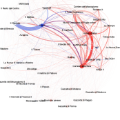
Year 2016

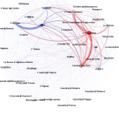
Fig. 1: Italian Audience-Duplication Networks obtained from the bipartite network of Italian news outlets and their Facebook commenters in 2015 (top) and 2016 (bottom). Node size is proportional to the news outlets’ engagement in terms of comments. Nodes are labelled with the name of the outlet and colored from red (left) to blue (right) according to the text-analysis political-leaning score computed following Gentzkow and Shapiro, (2010) and Garz et al., (2020). Edge width is proportional to the number of commenters in common between any two news outlets.

Figure 1 provides an illustrative example of both media bias and polarization starting from a preliminary analysis of the dataset described in Section 4. The figure displays a network of Italian news outlets in which the edges’ thickness is proportional to the number of Facebook commenters in common between any two outlets in the years 2015 (top) and 2016 (bottom). While media bias, in terms of political leaning, can be inferred indirectly from the network’s structure or directly by analyzing news outlets’ content production, an increase in polarization can be detected when the average number of users interacting with various sources decreases (see Figure 2).

Media bias entails the propagation of biased news pieces, the aim of which is often to support the interest of some individuals or groups, such as political parties. The phenomenon is considered detrimental to consumer welfare (Gentzkow et al., 2015) as it entails a reduction in the informativeness of news pieces, while some argue that biased news outlets jointly driven by ideological interests and profits could even affect political outcomes (Anderson and McLaren, 2012). Recent advancements in measuring media bias include the implementation of text-analysis techniques to take into account the similarity between news articles and political content (see Gentzkow and Shapiro, 2010; Garz et al., 2020) and the use of latent-space models (Hoff et al., 2002; Friel et al., 2016; Sewell and Chen, 2016) to obtain a political leaning measure from social-media relational data (Barberá, 2015 and Ng et al., 2021).

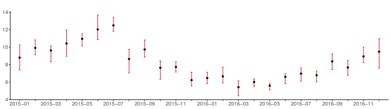
Fig. 2: Monthly network density of the average number of commenters in common between any two outlets. Red bars display the inter-quartile range and black dots denote the median.

Polarization refers to the radicalization of people’s opinions in the sense that they are further apart. Some fear that this change in attitudes may be reflected in more partisan positions of people’s representatives even though there is no obvious evidence of this (Prior, 2013). Others claim that online social media exacerbate polarization by offering incentives for homophilous behavior, i.e. the tendency to interact with similar individuals (Dandekar et al., 2013). However, while a predisposition toward homophily has been observed on several social platforms (see Hanusch and Nölleke, 2019; Cinelli et al., 2021), evidence of an exacerbation of polarization in social media environments is mixed (Kubin and von Sikorski, 2021). Several different methodologies have been adopted for measuring polarization (see Esteban and Ray, 1994; Yarchi et al., 2021), including in the field of network science (see Garimella et al., 2018; Cinelli et al., 2021). Two common objects of investigation are bipartite networks, relating social media users to online pages, and audience duplication networks, in which nodes represent pages and weighted edges denote the number of users in common between any pair of pages. Figure 3 illustrates the two concepts.

Previous studies about media polarization use heuristics to detect communities and informal sequential analysis for time variation, while we propose a formal statistical framework for dynamic polarization analysis.

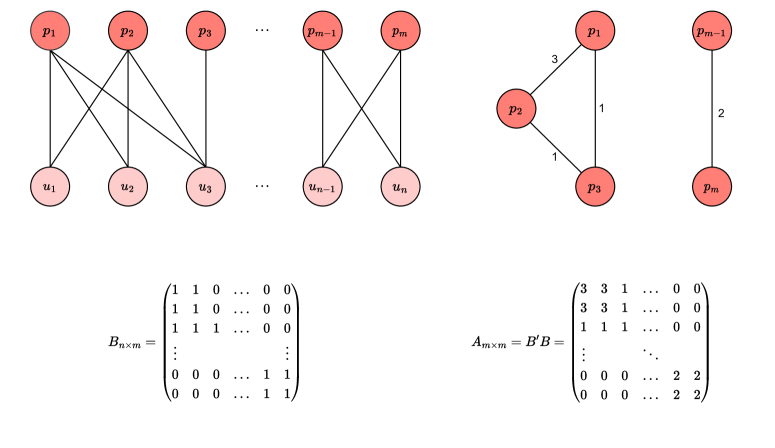
Fig. 3: Media Networks: An example of a bipartite network of $n$ readers, $u_{1},\ldots,u_{n}$ and $m$ news outlets, $p_{1},\ldots,p_{m}$ (top left) and the corresponding audience duplication network obtained using one-mode projection (top right). At the bottom, the adjacency-matrix representation of both the bipartite network, $B_{n\times m}$, and the audience-duplication network $A_{m\times m}$. The matrix $A$ is obtained as $A=B^{\prime}B$.

In particular, we introduce a novel dynamic Latent-Space (LS) network model which exploits both time-varying online audience-duplication network data and textual content to characterize a set of news outlets both in terms of a dynamic latent political-leaning dimension and in terms of popularity via individual effects.

LS models (Hoff et al.,, 2002) project the nodes of a network on a lower $d$-dimensional latent space. Extensions of the original model include e.g. a dynamic component for the latent coordinates (Friel et al.,, 2016; Sewell and Chen,, 2016; Kim et al.,, 2018), mixtures of latent coordinates (see Handcock et al.,, 2007) or extensions to multi-layer networks (see Gollini and Murphy,, 2016; D’Angelo et al.,, 2019; Sosa and Betancourt,, 2022). The statistical properties of LS models have been addressed by Rastelli et al., (2016) for binary networks, while Barberá, (2015) presents an early application of LS modeling for the estimation of latent ideology on social media and De Nicola et al., (2023) provides a static assessment of media polarization using LS models.

Our paper adds to the methodological literature in several respects:

• The latent coordinates of our LS model provide a novel measure of media bias which combines information from network data (e.g. Barberá,, 2015) and from a state-of-the-art text-based indicator (e.g. Gentzkow et al.,, 2015; Garz et al.,, 2020);

• We endow the latent coordinates with Markov-Switching (MS) dynamics which allows for capturing polarization regimes over time. The choice of modeling regimes rather than trajectories of polarization is coherent with the literature on opinion formation (see Iyengar et al.,, 2012; Törnberg et al.,, 2021). In addition, the MS is parsimonious and more easily scalable than other dynamic specifications.

• We extend the results of Rastelli et al., (2016) on statistical properties of LS models to weighted temporal networks with MS dynamics (MS-LS models) by obtaining closed-form expressions for the first and second moment of the strength distribution. Besides the theoretical relevance of the results, we show how such closed-form expressions can be used to assess the adequacy of the proposed model against other competing models (See Section 4.3).

Our model is applied to a novel time-varying network dataset we obtained from the Facebook daily online activity of a broad set of news outlets from four European countries (France, Germany, Italy, and Spain) in the years 2015 and 2016. This provides estimates of media bias that are coherent with the PEW Research survey (Mitchell et al.,, 2018). We also shed light on the in-platform (i.e. within Facebook) polarization regimes across the four countries. We find evidence of cross-country heterogeneity in the shifts from low to high polarization regimes, in line with the sociological argument of Prior, (2013). The newly constructed dataset is freely available (see Appendix J).

Section 2 will be dedicated to the overall description of the model within a Bayesian setup and to the discussion of the statistical properties of the model. In Section 3, we discuss posterior inference along with the constraints used in our model and present a simulation exercise. Finally, Section 4 describes the dataset of European news outlets and applies our model in both a static and a dynamic setup.

2 The Longitudinal Markov-Switching Latent Space Model

2.1 The Model

Let $\mathcal{G}=\{\mathcal{G}_{rt},r=1,2,\ldots,R,\,t=1,2,\ldots,T_{r}\}$ be an undirected and weighted temporal (in our application audience-duplication) network with multiple layers $\mathcal{G}_{rt}=(V_{rt},E_{rt},Y_{rt})$. For each layer (country) $r$, the vertex set (collection of news outlets) is constant, i.e. $V_{rt}=V_{r}\subset\mathbb{N}$, and the edge set $E_{rt}\subset V_{r}\times V_{r}$ (common commenters between any two outlets) is time-varying. For each edge $(i,j)\in E_{rt}$ we assume the $(i,j)$-th element of the weighted adjacency matrix $Y_{rt}$, i.e. $Y_{ijrt}$, is observed and denotes the number of connections (commenters in common) between news outlets $i$ and $j$ at time $t$ in country $r$. We adopt a Poisson model for the connections:

$$Y_{ijrt}\stackrel{{\scriptstyle ind}}{{\sim}}\mathcal{P}oi(\lambda_{ijrt}),$$ (1)

for $i,j=1,\ldots,N_{r}$, $t=1,\ldots,T_{r}$ and $r=1,\ldots,R$, where $N_{r}=Card(V_{r})$ is the number of nodes in layer $r$ and $\mathcal{P}oi(\lambda)$ denotes a Poisson distribution with intensity parameter $\lambda>0$. In our LS model, the intensity is driven by static ($\alpha_{ir}$) and $d$-dimensional dynamic node-specific latent features ($\mathbf{x}_{irt}\in\mathcal{X}\subset\mathbb{R}^{d}$):

$$\log\lambda_{ijrt}=\alpha_{ir}+\alpha_{jr}-\beta_{r}||\mathbf{x}_{irt}-\mathbf{x}_{jrt}||^{2}.$$ (2)

The parameters $\alpha_{ir}$, $i=1,\ldots,N_{r}$ have the natural interpretation of individual effects which are news-outlet specific and capture the popularity of the outlet (the engagement of the audience with the newspaper). The latent variables $\mathbf{x}_{irt}$, $i=1,\ldots,N_{r}$ enter the log intensity through the squared Euclidean distance as suggested in Gollini and Murphy, (2016) and in D’Angelo et al., (2019). This accounts for a clearer representation of the proximity of news outlets on a latent manifold and leads to faster computational convergence compared to the standard Euclidean distance. Assuming $\beta_{r}>0$ lends an interpretation of similarity features to the latent variables. The more similar the news outlets (the closer the nodes), the higher the number of commenters they tend to have in common.

We also employ an observable political leaning proxy, $\ell_{irt}$, to provide additional information on the location of news outlets within the latent space. Our modeling choice is to not include $\ell_{irt}$ in the log-intensity equation to preserve the tractability of the random graph model properties. Rather we assume that the political-leaning proxy $\ell_{irt}$ is driven by the same latent variables $\mathbf{x}_{irt}$ as appear in the network log-intensity:

$$\ell_{irt} \stackrel{{\scriptstyle ind}}{{\sim}} \mathcal{B}e(\varphi(\gamma_{0r}+\bm{\gamma}_{1r}^{\prime}\mathbf{x}_{irt})\phi_{r},(1-\varphi(\gamma_{0r}+\bm{\gamma}_{1r}^{\prime}\mathbf{x}_{irt}))\phi_{r}),$$ (3)

where $\mathcal{B}e$ denotes the Beta distribution while $\varphi(x)=1/(1+\exp(-x))$ is the logistic function, so that $\varphi(\gamma_{0r}+\bm{\gamma}_{1r}^{\prime}\mathbf{x}_{irt})$ is the expectation of $\ell_{irt}$ and $\phi_{r}>0$ is a precision parameter. This modeling choice allows us to endow the latent features $\mathbf{x}_{i,rt}$ with a media-bias interpretation while ensuring $y_{ijrt}$ is independent of $\ell_{irt}$ conditional on $\mathbf{x}_{irt}$. Thus, we can interpret the latent space as the political spectrum of news outlets.

To make our model dynamic, we assume that a Markov-Switching (MS) process drives the dynamic latent features. For this reason, we assume the existence of a Hidden Markov Chain with $K_{r}<\infty$ possible states of the world. The MS process allows our latent features $\mathbf{x}_{irt}$ to vary jointly through time across the different states. In the media environment, one can e.g. think about a state of low polarization, where news outlets are perceived, on average, closer within the political spectrum, and a state of high polarization, in which news outlets are perceived politically further apart (e.g., see Macy et al., (2021); Leonard et al., (2021) on polarization dynamics). We can reparameterize our dynamic latent features $\mathbf{x}_{it}$ to account for this MS dynamic:

$$\mathbf{x}_{irt}=\sum_{k=1}^{K_{r}}\mathbb{I}(s_{rt}=k)\bm{\zeta}_{ikr},$$ (4)

where $\bm{\zeta}_{ikr}$ denotes the latent position of news outlet $i$ of country $r$ in state $k$, while $\mathbb{I}(s_{rt}=k)$ is an indicator function which is 1 if the observed state $s_{rt}=k$ for country $r$ at time $t$, and 0 otherwise. Moreover, we characterize the transition between states through:

$$\mathbb{P}(s_{rt}=k|s_{r,t-1}=l)=q_{lkr},\,l,k=1,\ldots,K_{r},$$ (5)

which can be grouped in the transition probability matrix $\mathbf{Q}_{r}=\{\bm{q}_{1r},\ldots,\bm{q}_{kr},\ldots,\bm{q}_{K_{r}r}\}$, where $\bm{q}_{kr}=\left(q_{k1r},\ldots,q_{kK_{r}r}\right)$ denotes a column vector such that $\bm{q}^{\prime}_{kr}\mathbf{1}=1$ for each state $k$.

The use of a large number of parameters can produce over-fitting. Thus, we take a Bayesian approach to inference and choose the following prior structure (as explained in Section 3.2 we fix $\beta_{r}$ in our empirical application):

$$\pi(\alpha_{1r},\dots,\alpha_{N_{r}r},\{\bm{\zeta}_{1kr},\dots,\bm{\zeta}_{N_{r}kr},\sigma_{kr}^{2}\}_{k=1,\dots,K_{r}},\gamma_{0r},\gamma_{1r},\phi_{r},\mathbf{Q}_{r})=$$

$$\pi(\gamma_{0r})\pi(\gamma_{1r})\pi(\phi_{r})\left(\prod_{i=1}^{N_{r}}\pi(\alpha_{ir})\right)\prod_{k=1}^{K_{r}}\pi(\sigma_{kr}^{2})\pi(\bm{q}_{kr})\prod_{i=1}^{N_{r}}\pi(\bm{\zeta}_{ikr}|\sigma_{kr}^{2}),$$ (6)

where we find it useful to augment the parameter space with $\sigma_{kr}^{2},k=1,\dots,K_{r}$ and the specific prior distributions assumed are detailed in Appendix C.1. In our implementation of the model with $d=1$ and $K=2$, we have little prior information at our disposal and we opt for the use of relatively vague priors to let the data speak. Our results are robust to substantial changes in these priors.

The directed acyclic graph in Figure 4 summarizes our MS-LS model.

Fig. 4: Directed Acyclic Graph of the Markov-switching latent-space model. The graph exhibits the conditional independence structure of the observation model for $y_{ijrt}$ and $\ell_{irt}$ within white circles with parameters, $\bm{\alpha}_{r}=\{\alpha_{1},\ldots,\alpha_{N_{r}}\}$, $\beta_{r}$, $\gamma_{0r}$, $\bm{\gamma}_{1r}$, $\phi_{r}$, latent coordinates $\mathbf{x}_{rt}=\{\mathbf{x}_{1rt},\ldots,\mathbf{x}_{N_{r}rt}\}$, their state-dependent counterparts $\bm{\zeta}_{kr}=\{\bm{\zeta}_{1kr},\ldots,\bm{\zeta}_{N_{r}kr}\}$ with variance $\sigma^{2}_{kr}$, and latent states, $s_{rt}$, within grey circles.

2.2 Model Properties

We now present some of the properties of the MS-LS Model in (1), (2) and (4). With Assumption 2.1, we extend the scope of the Latent Variable Model provided in Rastelli et al., (2016) to weighted temporal networks. To enhance readability, we drop the country index $r$. In addition, we do not consider the political-leaning equation (3) since this is quite specific to our application and we aim to present the properties of a general network model.

Assumption 2.1.

Given an undirected temporal network, $\mathcal{G}_{t}=(V,E_{t})$, for $t=1,2,\ldots$ having vertex set $V\subset\mathbb{N}$ and weighted edge sets $E_{t}\subset V\times V$ with characteristic weight $Y_{ijt}$, we assume a sequence of latent coordinates $\{X_{1t},\ldots,X_{Nt}\}$ for $t=1,2,\ldots$ with $X_{it}\in\mathcal{X}\subset\mathbb{R}^{d}$ for each node $i\in V$ and time index $t\in\mathbb{N}$.

With Assumption 2.2, we introduce the Markov-Switching dynamics.

Assumption 2.2.

Given a $K$-state latent Markov-chain process $s_{t}\in\{1,2,\ldots,K\}$ for $K<\infty$ and $t=1,2,\ldots$ with transition probabilities $q_{lk}=\mathbb{P}(s_{t}=k|s_{t-1}=l)$, we assume the latent variables $X_{it}=\sum_{k=1}^{K}\mathbb{I}(s_{t}=k)Z_{ik}$. We also define the set $\mathscr{Z}_{k}=\{\zeta_{1k},\ldots,\zeta_{Nk}\}$ consisting of the i.i.d. realizations of the latent random variables $\{Z_{1k},\ldots,Z_{Nk}\}$ with $k\in\{1,\ldots,K\}$, where each $Z_{ik}$ is distributed according to $\pi_{k}(\cdot)$, a given probability measure.

Assumption 2.3 introduces the conditional independence between any two edges given the latent variables and the current state of the world.

Assumption 2.3.

We assume conditional independence between any two edges given the latent variables applicable to the current state $s_{t}$. Hence, $\forall(j,i)\in E_{t}$, $Y_{ijt}|X_{it},X_{jt}\sim\mathcal{P}oi\left(\lambda_{ijt}\right)$ is a Poisson random variable with intensity parameter $\lambda_{ijt}$.

Moreover, we assume that our set of latent variables is jointly normally distributed.

Assumption 2.4.

The latent variables are normally distributed: $Z_{ik}|\sigma_{k}^{2}\sim\mathcal{N}(\bm{0},\sigma_{k}^{2}I_{d})$ and take values in $\mathbb{R}^{d}$, for a fixed $d$.

Finally, we specify the form of the intensity parameter $\lambda_{ijt}$.

Assumption 2.5.

Given the individual effects $\alpha_{i}$ and $\alpha_{j}$ and the latent variables, we assume the Poisson rate parameter:

$$\lambda_{ijt}=\exp\left\{\alpha_{i}+\alpha_{j}-\sum_{k=1}^{K}\mathbb{I}(s_{t}=k)\beta||\zeta_{ik}-\zeta_{jk}||^{2}\right\}$$

Under Assumptions 2.1-2.5 our model is a time-varying MS-LS model with Poisson weights and normally distributed latent variables.

The nodal strength, defined as $Y_{it}=\sum_{j\neq i}Y_{ijt}$, is a quantity of particular interest when dealing with weighted networks as it provides information on how strongly connected a node is with its neighbors. We can derive the following properties of the probability generating function (pgf) of the nodal strength, where in the sequel we will focus on the strength of a random node (and, thus, omit the index $i$):

Proposition 2.1.

The $m$-th derivative of the conditional pgf $G_{l}$ of the nodal strength evaluated in $x=1$ given $s_{t-1}=l$ for the MS-LS model can be written as:

$$\footnotesize\left.\frac{\partial^{m}G_{l}(x)}{\partial x^{m}}\right|_{x=1}=\sum_{k=1}^{K}q_{lk}\left.\frac{\partial^{m}\widetilde{G}_{k}(x)}{\partial x^{m}}\right|_{x=1}=\sum_{k=1}^{K}\sum_{\underline{h}_{i}\in\mathcal{H}_{i}}\binom{m}{\underline{h}_{i}}e^{\sum_{j\neq i}(\alpha_{i}+\alpha_{j})h_{j}}(\sigma^{2}_{k})^{-\frac{d}{2}}b_{\underline{h},k}q_{lk}$$

where $\widetilde{G}_{k}(x)$ is the conditional pgf given $s_{t}=k$ and $s_{t-1}=l$ and

$$b_{\underline{h},k}=\left(\frac{1}{\sigma^{2}_{k}}+\sum_{j\in\mathcal{N}_{i}}\frac{2\beta h_{j}}{2\beta h_{j}\sigma^{2}_{k}+1}\right)^{-\frac{d}{2}}\prod_{j\in\mathcal{N}_{i}}\left(2\beta h_{j}\sigma^{2}_{k}+1\right)^{\frac{d}{2}}$$

with multi-index $\underline{h}_{i}=\{h_{1},\ldots,h_{i-1},h_{i+1},\ldots,h_{N}\}$ and index set $\mathcal{H}_{i}=\{h_{j}\in\{0,\ldots,m\},\quad j\neq i|\sum_{j\neq i}h_{j}=m\}$, $\mathcal{N}_{i}=\{j|j\neq i,h_{j}>0\}$ and $\beta>0$.

The first derivative of the pgf returns the conditional expectation of the strength for a random node, $\mathbb{E}(Y_{t}|s_{t-1}=l)$.

Corollary 2.1.

Defining $\alpha=\alpha_{i}+\alpha_{j}$ for each $i$ and each $j$, the expected nodal strength of the underlying network $\mathcal{G}_{t}$ can be expressed as

$$\mathbb{E}(Y_{t}|s_{t-1}=l)=\left.G_{l}^{\prime}(x)\right|_{x=1}=\sum_{k=1}^{K}q_{lk}\left.\widetilde{G}_{k}^{\prime}(x)\right|_{x=1}=(N-1)e^{\alpha}\sum_{k=1}^{K}q_{lk}\left(4\sigma_{k}^{2}\beta+1\right)^{-\frac{d}{2}}.$$

Note that $\mathbb{E}(Y_{t}|s_{t-1}=l)$ turns out to be a weighted sum of the expected nodal strength obtained by conditioning on each possible state of the world. The result in Rastelli et al., (2016) can be obtained as a special case imposing all but one of the conditional probabilities $q_{lk}$ for $k\in\{1,\ldots,K\}$ to be zero. This is due to the fact that the expected conditional strength in their unweighted network is the same as in our setup, only with the restriction that $\alpha$ has to be negative. The expected strength for each regime increases linearly with the number of nodes, $N$, and exponentially with the intercept parameter $\alpha$. The lower $\sigma^{2}_{k}\beta$, the larger the similarity between the nodes in that state and, in turn, the higher the expected strength.

Corollary 2.2.

The analytical expression of the variance of the strength distribution uses the first and the second factorial moment of the pgf, resulting in

$$Var(Y_{t}|s_{t-1}=l)=\sum_{k=1}^{K}q_{lk}Var(Y_{t}|s_{t}=k)+\sum_{k=1}^{K}q_{lk}\left(\left.\widetilde{G}_{k}^{\prime}(x)\right|_{x=1}-\left.G_{l}^{\prime}(x)\right|_{x=1}\right)^{2},$$

where $Var(Y_{t}|s_{t}=k)=\left.\widetilde{G}_{k}^{\prime\prime}(x)\right|_{x=1}+\left.\widetilde{G}_{k}^{\prime}(x)\right|_{x=1}-\left.\widetilde{G}_{k}^{\prime 2}(x)\right|_{x=1}$.

Similarly, an analytical expression for the Dispersion Index can be obtained:

$$\mathfrak{D}(Y_{t}|s_{t-1}=l) =\sum_{k=1}^{K}q_{lk}\mathfrak{D}(Y_{t}|s_{t}=k)+v,$$

where

$$\mathfrak{D}(Y_{t}|s_{t}=k) =1+v_{k}-\left.\widetilde{G}_{k}^{\prime}(x)\right|_{x=1},\quad v=\frac{\sum_{k=1}^{K}q_{lk}\left.\widetilde{G}_{k}^{\prime\prime}(x)\right|_{x=1}}{\sum_{k=1}^{K}q_{lk}\left.\widetilde{G}_{k}^{\prime}(x)\right|_{x=1}}-\sum_{k=1}^{K}q_{lk}v_{k},$$

with $v_{k}=\left.\widetilde{G}_{k}^{\prime\prime}(x)/\widetilde{G}_{k}^{\prime}(x)\right|_{x=1}$. The derivatives $\widetilde{G}_{k}^{\prime}(x)$ and $\widetilde{G}_{k}^{\prime\prime}(x)$ are defined in (A.1) and (A.2) in Appendix A.

The result for the second factorial moment differs from the results in Rastelli et al., (2016) as our derivation reflects the existing heterogeneity in weighted edges. As expected, due to the equal-dispersion property of the Poisson distribution, both the mean and variance of the strength distribution increase with the intercept value $\alpha$.

We derive the above results in Appendix A along with a sensitivity analysis of the moments of the strength distribution to different combinations of the model parameters.

3 Inference

3.1 Posterior sampling algorithm

In this section, we will go back to the setup in (1)-(6), so including (3), and assume $d=1$ in line with the particular application we focus on, so that $\mathbf{x}_{irt}$ and $\bm{\gamma}_{1}$ are scalars $x_{irt}$ and $\gamma_{1}$. Let $\mathbf{Y}=(\mathbf{Y}_{1},\ldots,\mathbf{Y}_{R})$ where $\mathbf{Y}_{r}=(\mathbf{Y}_{1r},\ldots,\mathbf{Y}_{T_{r}r})$ be the collection of observed network weights with characteristic element $Y_{ijrt}$, $\bm{\ell}=(\bm{\ell}_{1},\ldots,\bm{\ell}_{R})$ where $\bm{\ell}_{r}=(\bm{\ell}_{1r},\ldots,\bm{\ell}_{T_{r}r})$ are the observable political-leaning proxies with characteristic element $\ell_{irt}$ and $\mathbf{s}_{r}=(s_{r1},\ldots,s_{rT_{r}})$ are the latent states for each country $r$. Consider the parameters $\bm{\theta}=\left(\bm{\theta}_{1},\ldots,\bm{\theta}_{R}\right)$ where $\bm{\theta}_{r}=\left(\bm{\alpha}_{r},\bm{\zeta}_{r},\bm{\sigma}^{2}_{r},\gamma_{0r},\gamma_{1r},\phi_{r},\bm{Q}_{r}\right)$, while $\beta_{r}$ is fixed in our empirical implementation (see Section 3.2). Here $\bm{\zeta}_{r}=(\bm{\zeta}_{1r},\ldots,\bm{\zeta}_{ir},\ldots,\bm{\zeta}_{N_{r}r})$ denotes the latent parameters, where $\bm{\zeta}_{ir}=(\zeta_{i1r},\ldots,\zeta_{iK_{r}r})$, a row vector with $K_{r}$ elements, while $\bm{\sigma}^{2}_{r}=(\sigma^{2}_{1r},\ldots,\sigma^{2}_{K_{r}r})$. The joint posterior $p(\bm{\theta}|\mathbf{Y},\bm{\ell})$ $\propto f(\mathbf{Y},\bm{\ell}|\bm{\theta})\pi(\bm{\theta})$ is not tractable. Thus we follow a data augmentation approach and apply a Gibbs sampler for posterior inference (see Appendix C). Let us denote with $\bm{\xi}_{r}=(\bm{\xi}_{1r},\ldots,\bm{\xi}_{T_{r}r})$ the collection of state indicator variables, where $\bm{\xi}_{rt}=(\xi_{1rt},\ldots,\xi_{K_{r}rt})^{\prime}$ and $\xi_{krt}=\mathbb{I}(s_{rt}=k)$. Then, the complete-data likelihood function for $r=1,\ldots,R$ is the product of the following:

$$f(\mathbf{Y}_{r},\bm{\ell}_{r},\bm{\xi}_{r}|\bm{\theta}_{r})=\prod_{t=1}^{T_{r}}\prod_{i=1}^{N_{r}}\left(f_{B}(\ell_{irt}|s_{rt},\bm{\theta}_{r})\prod_{j=i+1}^{N_{r}}f_{P}(Y_{ijrt}|s_{rt},\bm{\theta}_{r})\right)\prod_{l=1}^{K_{r}}\prod_{k=1}^{K_{r}}q_{lkr}^{\xi_{lrt-1}\xi_{krt}},$$ (7)

where $f_{P}(Y_{ijrt}|s_{rt},\bm{\theta}_{r})$ is the Poisson pmf in (1) with dynamic intensity given in (2), $f_{B}(\ell_{irt}|s_{rt},\bm{\theta}_{r})$ the Beta pdf given in (3). With this notation, $x_{irt}$ can be written as $\bm{\zeta}_{ir}\bm{\xi}_{rt}$, in (1) and (3).

We approximate the joint posterior distribution by Markov-chain Monte Carlo (MCMC) sampling. Our Gibbs sampling algorithm iterates the following steps for each $r$:

1. Draw $\alpha_{ir}$ from $p(\alpha_{r}|\ldots)$, $i=1,\ldots,N_{r}$ via Adaptive Metropolis-Hastings (MH);

2. Draw $\phi_{r}$ from $p(\phi_{r}|\ldots)$ via MH with truncated normal proposal;

3. Draw $\gamma_{0r}$ and $\gamma_{1r}$ from $p(\gamma_{0r},\gamma_{1r}|\ldots)$ via MH;

4. Draw $\zeta_{ikr}$ from $p(\zeta_{ikr}|\ldots)$, $i=1,\ldots,N_{r}$ and for $k=1,\ldots,K_{r}$ via Adaptive MH;

5. Draw $\sigma^{2}_{kr}$ from $p(\sigma^{2}_{kr}|\bm{\zeta}_{kr})$ for $k=1,\ldots,K_{r}$;

6. Draw $\bm{q}_{lr}$ from $p(\bm{q}_{lr}|\bm{\xi}_{r})$ for $l=1,\ldots,K_{r}$.

7. Draw $\mathbf{s}_{r}$ via the forward-filtering and backward-sampling algorithm (see Frühwirth-Schnatter,, 2006).

   Further details on the algorithmic design can be found in Appendix C.

3.2 Identifying Restrictions

The model presents well-known identification challenges. The first issue is related to the multiplication of the squared Euclidean distance $||\bm{\zeta}_{ir}\bm{\xi}_{rt}-\bm{\zeta}_{jr}\bm{\xi}_{rt}||^{2}$ by the parameter $\beta_{r}$. As there is a clear scale indeterminacy between $\beta_{r}$ and the variance of the latent variables in terms of $\sigma_{k}^{2}$, we choose to set $\beta_{r}=1$. In addition, latent coordinates enter the parameter $\lambda_{ijrt}$ only through the squared distance. This makes – in principle – positions that differ just by means of reflection, translation, and rotation equally likely (see Hoff et al.,, 2002 and Friel et al.,, 2016). Nonetheless, the introduction of (3) helps prevent the emergence of many equivalent latent-space representations. Still, translation and reflection along the $y$-coordinate remain possible. To overcome translation issues, we center the latent coordinates to the origin of the axes at each Gibbs-sampling iteration. To overcome reflection, we assume that the position of a single outlet is known in terms of left and right political leaning (e.g. $\zeta_{i^{*}kr}<0$ for a left-leaning outlet $i^{*}$ and for each state $k$), and we apply a reflection transformation to the latent leaning coordinates every time the latent leaning of $i^{*}$ is in the wrong orthant, similarly to Barberá, (2015). Finally, as pointed out in Frühwirth-Schnatter, (2006), the joint posterior in Markov-Switching models is invariant with respect to a re-labeling of the hidden states. We tackle this issue by imposing an ordering restriction on the latent regimes across states. In particular, we label latent regimes in increasing order of median distance, $\tilde{D}_{rk}=med_{j>i}\left(||\zeta_{ikr}-\zeta_{jkr}||\right)$.

3.3 Analysis of Simulated Data

We assess the performance of our inference method by running the algorithm on simulated data. Our simulation consists of 20 fictitious news outlets observed for 100 periods. Each period may belong to one of two polarization states $k\in\{L,H\}$, where State $L$ is characterized by a lower average distance in the political-leaning dimension across news outlets, and State $H$ has a higher average distance. So news outlets jointly undergo periods of high polarization and low polarization.

The latent leaning positions in State $H$, ${\zeta}_{iH}$, are drawn from a normal distribution centered at -$0.75$ for $i\in\{1,\dots,10\}$ and in $0.75$ for $i\in\{11,\dots,20\}$ with $\sigma_{H}=0.15$, while the latent leaning positions in State $L$, ${\zeta}_{iL}$, are centered around the positions -$0.25$ for $i\in\{1,\dots,10\}$ and $0.25$ for $i\in\{11,\dots,20\}$ with $\sigma_{L}=0.15$; the individual effect parameters $\alpha_{i}$ are randomly drawn from a normal distribution with $\mu_{\alpha}=0$ and $\sigma_{\alpha}=2$; the transition probability matrix $\bm{Q}$ has 0.95 on the diagonal and 0.05 as off-diagonal elements, and the sequence of states is randomly drawn from the Markov Chain initialized at State L; finally, we set $\phi=200$, $\gamma_{0}=-0.1$, and $\gamma_{1}=0.5$. We sample $Y_{ijt}$ and $\ell_{it}$ from the data generating process (1)-(4). Our simulation represents a situation in which news outlets diverge in magnitude – via $\alpha_{i}$ – and in terms of political leaning – via $\zeta_{ik}$.

We run our MCMC algorithm for 50,000 iterations and we discard the first 30,000 iterations as burn-in and thin by a factor of 10 to reduce auto-correlation in the draws. To correctly identify left and right-leaning, we consider news outlet 3 as known to be left.

Figure 5 reports a summary of the simulation results. From a comparison between the true values and the marginal posterior distributions, the model performs very well in terms of identification of the individual effects and latent variables (Panel A), the latent states (Panel B), as well as the other parameters in the simulation (Panel C). Credible regions for the pairs $(\alpha_{i},\zeta_{ik})$ estimated with our model (red solid ellipses in Panel A) are narrower than those obtained disregarding the political-leaning proxy $\ell_{it}$, i.e. dropping (3) from the model (dashed black ellipses). This suggests that the information-borrowing strategy is effective in improving the estimation accuracy of the latent variables. Properties of the MCMC chains are reported in the Supplementary Material (Appendix D). Our MCMC algorithm is implemented in R and C++ and we make the scripts freely available (see Appendix J.2).

4 Political Leaning and Polarization of News Outlets

We provide an application of our model to a dataset of daily Facebook activities related to 225 national and local news outlets in France, Germany, Italy and Spain. We provide both static and dynamic analyses which allow us to assess the media slant in these news outlets as well as the polarization levels and regimes across countries.

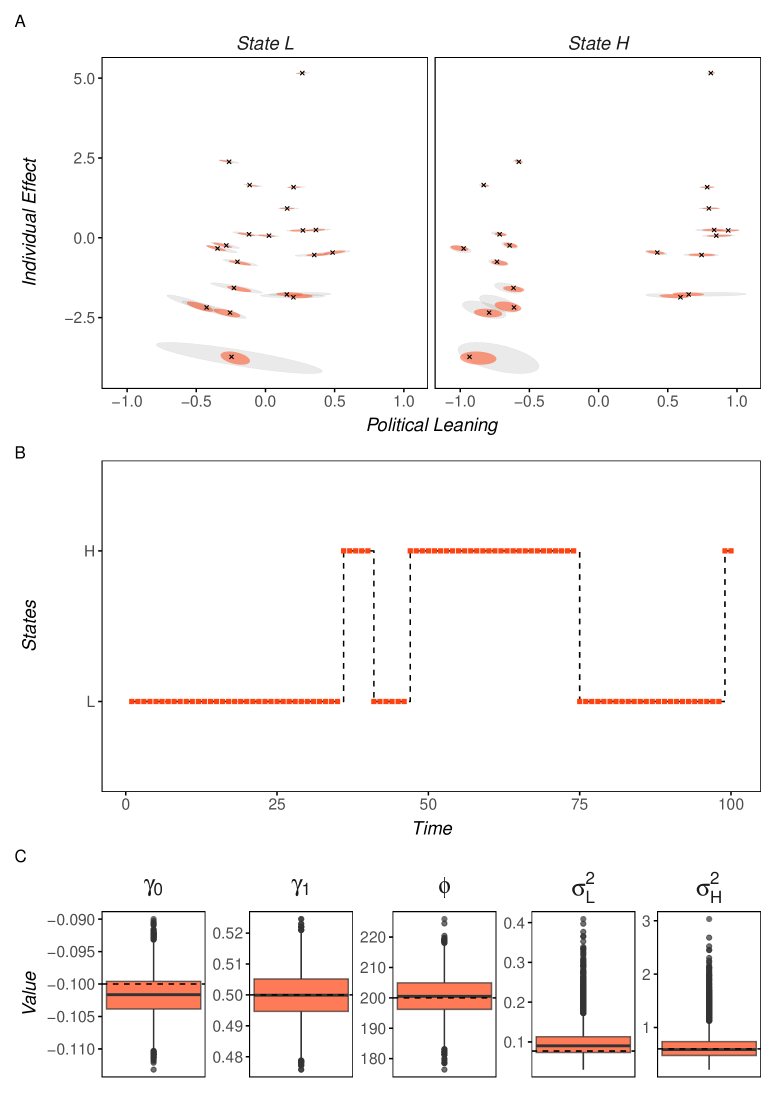
Fig. 5: Simulated data: Panel A: Estimated Coordinates in the Latent Leaning - Individual Effect Plane with 99% credible ellipses for the mode with (3) (solid red), without (3) (dashed black) and true values (crosses). Panel B: estimated latent states (red dots) and true states (dashed lines). Panel C: boxplots of the marginal posteriors for the parameters $\gamma_{0}$, $\gamma_{1}$, $\phi$, $\sigma^{2}_{L}$ and $\sigma^{2}_{H}$. The dashed lines indicate the true values.

4.1 Dataset Description and Construction

For our application, we construct and exploit a novel time-varying set of media networks, which we will call the network dataset. We build the networks from the source dataset collected by Schmidt et al., (2018) containing tick-by-tick information on the Facebook activity of national and local news outlets from four European countries (France, Germany, Italy, and Spain) in a time-span entirely covering the years 2015 and 2016. We aggregate this activity to daily data. The news outlet list is reported in the Reuters Digital News Report (2017) (Newman et al.,, 2017). The source dataset contains all posts published by the news outlets in those years along with the associated metadata and also all the data on anonymized user interactions with these posts in the form of comments. Table 1 reports a summary description of the source dataset, which includes for each country the set of news outlets’ pages, their posts and users’ comments.

Table 1: Source Dataset Description: Description of the Facebook dataset on national and local news outlets of the four European countries (France, Germany, Italy and Spain) gathered by Schmidt et al., (2018). The dataset entirely covers the years 2015 and 2016. The news outlet list is reported in the Reuters Digital News Report (2017).

Country	Pages	Posts	Comments	Commenters
France	65	1,008,018	47,225,675	5,755,268
Germany	49	749,805	31,881,407	5,338,195
Italy	54	1,554,817	51,515,121	4,086,351
Spain	57	1,372,805	34,336,356	6,494,725

After constructing the set of daily bipartite networks of interaction between news outlets and commenters - those Facebook users commenting on news outlets’ posts - for each country $r\in\{France,Germany,Italy,Spain\}$ at time $t$, we obtain the set of audience-duplication networks $\mathcal{G}_{tr}$ presented in Fig. 6 by performing the one-mode projection on the side of news outlets (as in Fig. 3).

We complement our network dataset with data from Crowdtangle (CrowdTangle Team,, 2022) and Chapel Hill Expert Survey (CHES) data (Polk et al.,, 2017). Crowdtangle allows retrieving Facebook posts for public pages and provides additional metadata for each post. In particular, the fields Link Text and Description contain information on the text of linked pages, such as the texts of news articles published on the Facebook walls of the news outlets. There is not a perfect match between all the pages available in the source dataset of Schmidt et al., (2018) and those available in Crowdtangle. Some news outlets may have changed account or ceased to exist. In this case, information about these news outlets may no longer be available on Facebook at the time of writing. The CHES questions political scientists on different aspects related to politics and European integration. The CHES dataset contains all the information at an aggregate level about scientists’ opinions on the ideological position of political parties in Europe. Here we will make use of the lrgen variable, which provides the ideological stance of a political party from 0 (extreme left) to 10 (extreme right). The information retrieved from Crowdtangle and CHES allows us to construct a text-analysis proxy for media slant. In particular, we obtain our observed proxy for daily media slant $\ell_{itr}$ by computing the index proposed by Gentzkow and Shapiro, (2010) and adapted to online media outlets by Garz et al., (2020). Such a media slant index relies on text analysis techniques to assess the similarity between pieces by news outlets and texts published by politicians. We then associate a political leaning to each news outlet as a function of this similarity and the parties’ political leaning. Further information on the adopted methodology can be found in Appendix F.

The network dataset and the media slant index are publicly available as described in Appendix J.1.

France	Germany	Italy	Spain

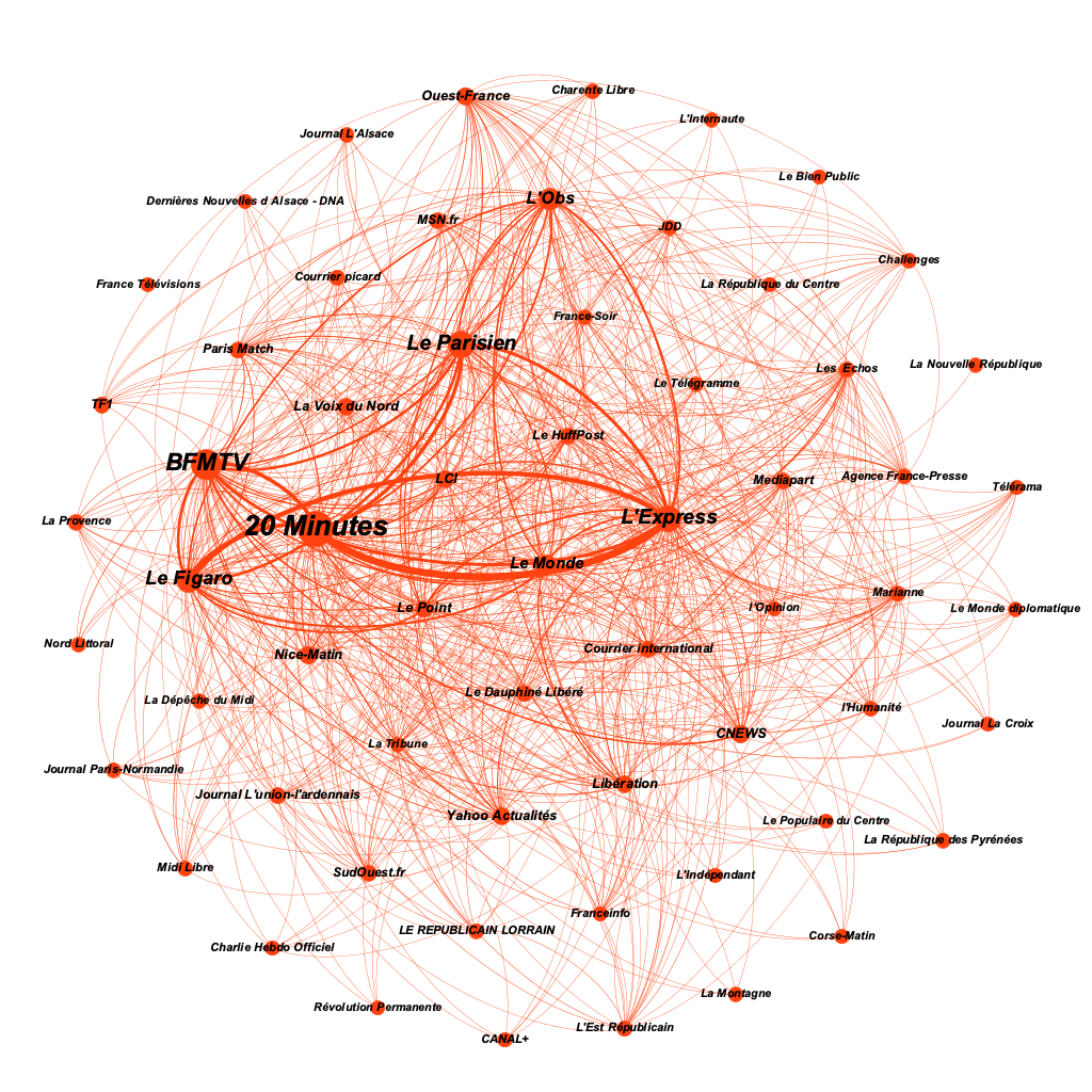
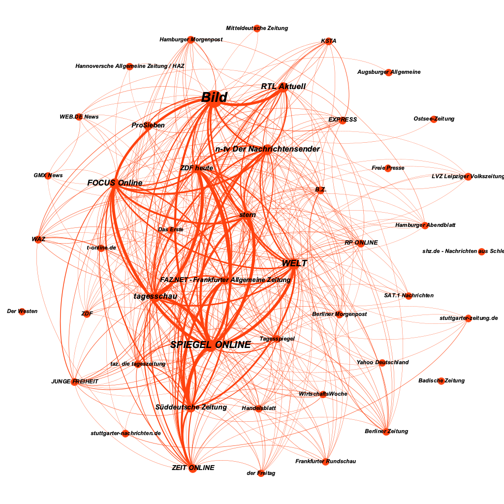
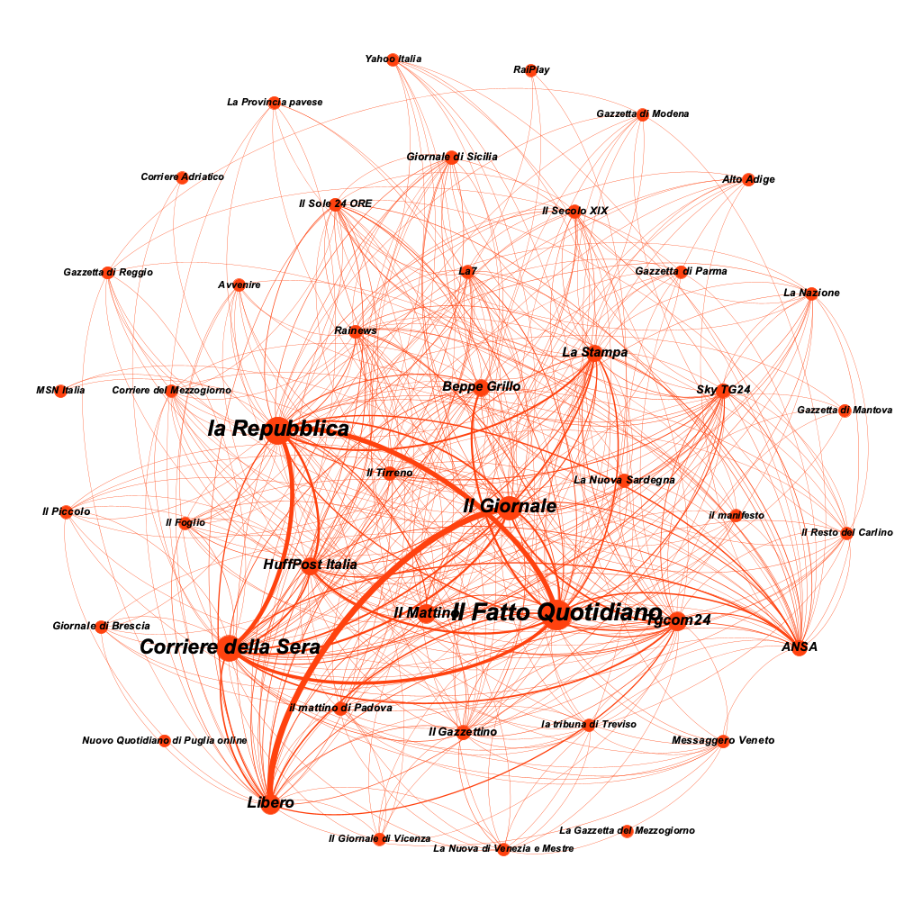
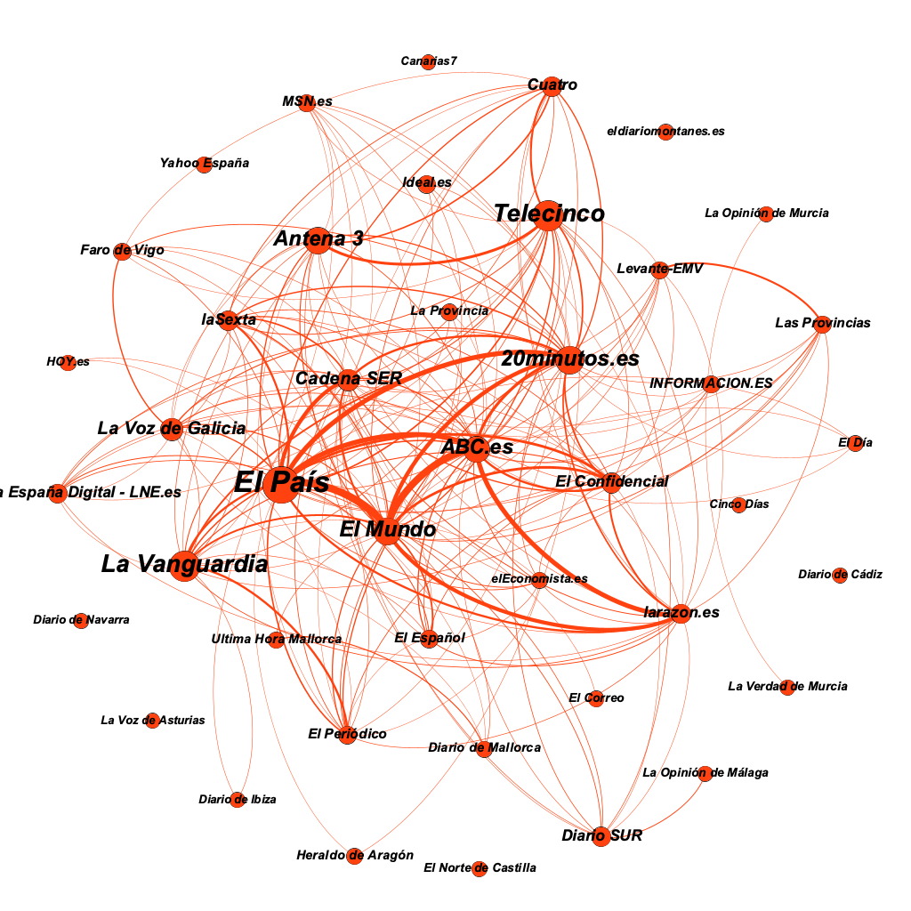
Fig. 6: Audience-Duplication Networks: Cumulative audience duplication network for France (top-left panel, 62 outlets), Germany (top-right panel, 47 outlets), Italy (bottom-left panel, 45 outlets) and Spain (bottom-right panel, 43 outlets) from January $1^{st}$ 2015 to December $31^{st}$ 2016. Node sizes are proportional to the cumulative number of comments received in the time interval, while edge thickness is proportional to the number of common commenters between each pair of outlets. Relevant quantities are normalized for each country.

4.2 Results from a Static Analysis

First, we implement a static version of our model on the whole 2-year time period, without the MS dynamic component. For this, we use an overall audience duplication network $\tilde{\mathcal{G}}_{tr}$, where the weighted edge for each pair of outlets is $\tilde{Y}_{ijr}=\sum_{t=1}^{T}Y_{ijrt}$, and the overall observable leaning-feature is constructed as $\tilde{\ell}_{ir}=T^{-1}\sum_{t=1}^{T}\ell_{itr}$. Panels A, B, C, and D in Fig. 7 report the estimated (posterior mean) latent coordinates in the latent leaning-individual effect space. We notice how the individual effect parameter $\alpha_{ir}$ associated with each news outlet and country may be interpreted in terms of news outlet’s engagement, as major national news outlets are concentrated at the top in each graph.

We correlate our posterior mean media slant with the results obtained by the PEW Research Survey (Mitchell et al.,, 2018). In this survey, participants were asked to assess the left-right leaning of national news outlets on a 0-6 scale with 0 indicating far left and 6 indicating far right. We will refer to the left-right ranking obtained by PEW Research as the PEW Research index. We find that the PEW Research index has a $0.73$ correlation with our estimated latent leaning, see Panel E in Fig. 7. Moreover, we notice the presence of both a left-leaning cluster (bottom-left) and a right-leaning cluster (top-right).

As a robustness check, we increase $d$ and assess whether considering a higher dimensional space has an impact on the agreement between the latent leaning and the PEW Research index. We notice that most of the information is retained by one single dimension and that the impact of considering one more latent dimension is negligible (see Fig. I.1 in the Appendix).

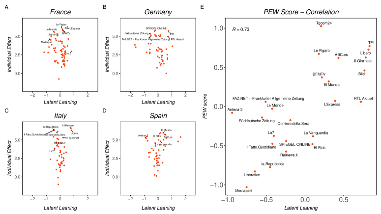
Fig. 7: PEW Index - Latent Leaning Static Comparison: Panels A, B, C, and D present the posterior mean of the latent coordinates of our news outlets, while Panel E displays the scatter plot comparing the PEW survey results with our estimated latent leaning variable (country-specific means have been subtracted from the PEW scores to improve readability).

Fig. I.2 in Appendix I presents the marginal posterior distribution of the parameters $\gamma_{0r}$, $\gamma_{1r}$ and $\phi_{r}$. The parameter $\gamma_{1r}$ conveys information on the relationship between the latent variable $x_{ir}$ and the observable leaning proxy $\ell_{ir}$. Latent leaning appears to be a strong driver for the observable proxy only in the case of Italy, as the posterior mass of $\gamma_{1r}$ is located far away from zero, while it seems a weak driver for France and mostly irrelevant for both Germany and Spain. Nonetheless, the strong correlation with the PEW Research index suggests that having information on online users’ interactions with news outlets may still be sufficient to provide an effective classification on the political spectrum.

4.3 Results from a Dynamic Analysis

We now estimate the model described in Subsection 2.1 in its dynamic specification, i.e. including the MS specification of (4). The dynamic analysis uses daily data, and we deleted from our dataset those outlets that remained inactive – i.e. did not receive any comment – for more than 15 consecutive days. Overall, we removed 13 news outlets (DE: 4 outlets, FR: 5, IT: 2, SP: 2, see Appendix G), who displayed unusual behavior. Posterior results for the parameters are presented in Figure 8, where it is clear that the large number of observations leads to more precise inference than in the static case. Inference on $\gamma_{1r}$ indicates a clear link between $x_{ir}$ and $\ell_{ir}$ for both France and Italy. Also, as expected, values of $\sigma_{H}^{2}$ tend to be larger than those for $\sigma_{L}^{2}$. In Fig. 9, we report the posterior means of the latent positions for the four countries in both states. The individual-effect values are coherent with the engagement interpretation in both states: well-known national newspapers appear in the upper part of the graph, while local newspapers are most prevalent at the bottom. Moreover, our latent variable also positively correlates with the PEW Research Survey Index in this setting. Figure 10 illustrates the correlation of 0.68 in the lower polarisation state and 0.69 in the state of higher polarisation.

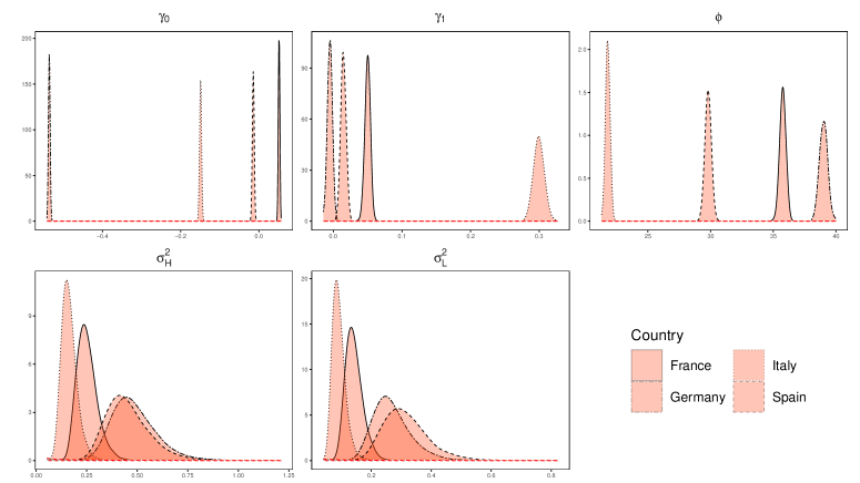
Fig. 8: Marginal Posteriors - Dynamic Analysis: Kernel posterior density estimates for the parameters $\gamma_{0r}$, $\gamma_{1r}$, $\phi_{r}$, $\sigma^{2}_{Lr}$ and $\sigma^{2}_{Hr}$ for France, Germany, Italy and Spain with prior pdfs indicated by red dashed lines (mostly indistinguishable from the horizontal axis).

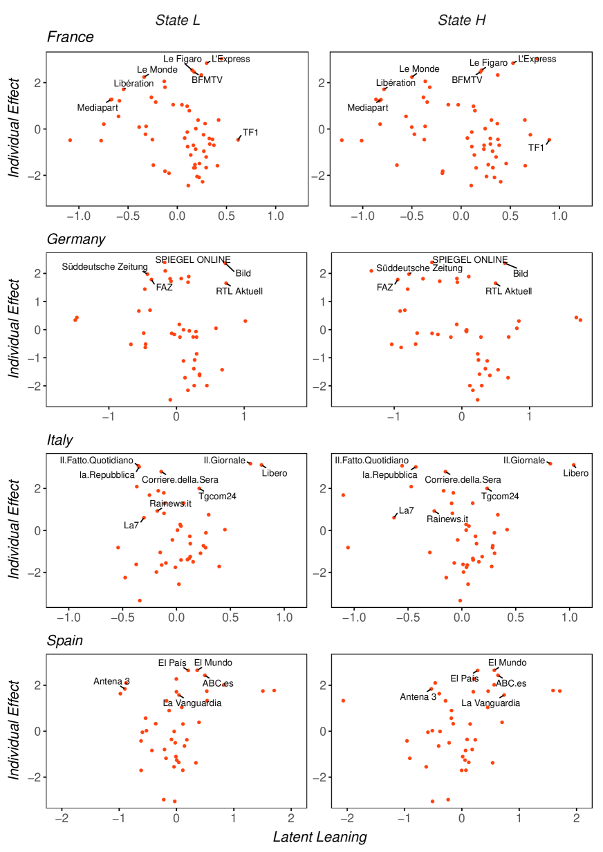
Fig. 9: Latent Positions - Dynamic Analysis: Posterior means of individual effects and latent coordinates of the news outlets for France (Panel A), Germany (Panel B), Italy (Panel C) and Spain (Panel D) in State $L$ and in State $H$.

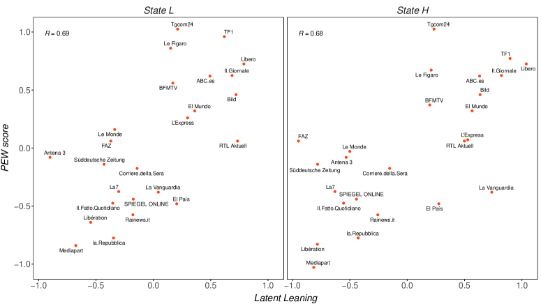
Fig. 10: PEW Index - Latent Leaning Dynamic Comparison: Scatter plot comparing the PEW survey results with the estimated latent leaning variable in State $L$ and $H$. The country-specific mean has been subtracted from the PEW Score to improve readability.

Table 2 reports a posterior predictive check (see Gelman et al.,, 2014) in which the posterior predictive expected nodal strength, nodal strength’s standard deviation and dispersion index – derived in Section 2.2 – are compared with the empirical values for the standard Poisson random graph model, the Poisson random graph model with individual effects and observed leaning distances and the MS-LS model. We notice how all models are able to mimic the first moment of the strength distribution, while the two more elaborate models are able to capture the observed dispersion in the strength distribution (with the MS-LS model giving a slightly better fit).

Latent states signal the presence of lower or higher in-platform polarization regimes. In state $L$ the average distance between outlets is lower in terms of political leaning than in state $H$, making Facebook users more prone to interact with news outlets with different political tendencies. Panels A-D of Fig. 11 report the estimated posterior probabilities for State $H$ through time for the four countries. We notice a tendency to move from a state of high in-platform polarization to a low polarization for Germany and Spain. Italy instead moves in the opposite direction, while France does not show a clear pattern, rather it alternates between the two states.

Overall, our findings contradict the hypothesis of a common shift toward a high polarization regime on social media in this time frame. Panels E-H of Fig. 11 report the estimated transition probabilities. Spain is characterized by high persistence whereas France switches most frequently between the two states.

Table 2: Network Posterior Predictive Check: The table compares the network characteristics in terms of expected strength, strength’s standard deviation, and dispersion index for the standard Poisson random graph model (second panel), the Poisson random graph model with individual effects and observed leaning distances as a covariate (third panel) and the dynamic latent space network model (bottom panel) with the observed network metrics averaged over time (top panel). The 95% credible intervals are in parenthesis.

	Average Empirical Network Metrics
	France	Germany	Italy	Spain
Expected Strength	280.83	161.82	380.98	239.32
S.D. Strength	450.53	209.39	600.58	340.76
Dispersion Index	814.20	306.11	1037.82	562.56
	R.G. $\lambda_{ijt}=\exp\{\alpha\}$
Expected Strength	280.82 (280.55, 281.10)	161.82 (161.56, 162.04)	380.99 (380.62, 381.37)	239.30 (239.00, 239.59)
S.D. Strength	16.53 (16.43, 16.62)	12.49 (12.40, 12.57)	19.17 (19.04, 19.29)	15.18 (15.07, 15.28)
Dispersion Index	0.98 (0.97, 0.99)	0.98 (0.96, 0.99)	0.98 (0.96, 0.99)	0.98 (0.96, 0.99)
	R.G. $\lambda_{ijt}=\exp\{\alpha_{i}+\alpha_{j}-\beta||\ell_{it}-\ell_{jt}||^{2}\}$
Expected Strength	276.64 (276.36, 276.92)	162.73 (162.47, 163.00)	375.68 (375.26, 376.09)	239.50 (239.19, 239.80)
S.D. Strength	431.33 (430.84, 431.85)	201.97 (201.60, 202.30)	577.62 (576.89, 578.30)	312.12 (311.67, 312.54)
Dispersion Index	672.57 (671.57, 673.75)	250.68 (250.10, 251.23)	888.15 (886.72, 889.50)	406.79 (405.96, 407.55)
	Dynamic MS-LS Model ($\mathcal{M}_{1r})$
Expected Strength	280.84 (280.60, 281.09)	161.81 (161.57, 162.03)	380.99 (380.64, 381.36)	239.32 (239.00, 239.64)
S.D. Strength	437.96 (437.52, 438.44)	201.90 (201.59, 202.24)	587.77 (587.12, 588.43)	313.64 (313.16, 314.13)
Dispersion Index	683.13 (682.10, 684.22)	251.94 (251.33, 252.54)	906.83 (905.48, 908.02)	411.12 (410.20, 412.04)

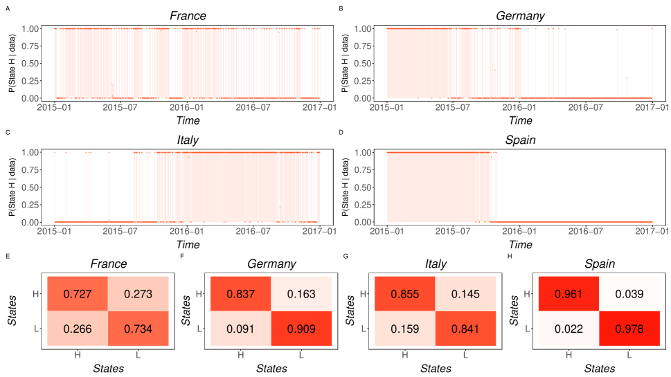
Fig. 11: Latent States Comparison: Posterior Probabilities for State H through time for France, Germany, Italy and Spain (Panels A-D). Posterior mean transition matrices for France, Germany, Italy and Spain (Panels E-H) with red shades proportional to the magnitude of the transition probability.

4.4 Model Selection

We perform model selection considering three alternative models: $\mathcal{M}_{1r}$ is the unrestricted model described in Subsection 2.1, $\mathcal{M}_{2r}$ omits the text-analysis interpretation in (3) (equivalent to imposing $\gamma_{1r}=0$) for each country $r$, while the static model $\mathcal{M}_{3r}$ omits the Markov-switching dynamics described in (4). This comparison highlights the contributions of the observable leaning a-là Gentzkow et al., (2015) and the dynamic component.

Model selection is carried out via two popular predictive measures, the Deviance Information Criterion (DIC) (Spiegelhalter et al.,, 2002) and the log pointwise predictive density (lppd) of Gelman et al., (2014) (see Appendix E for further details). Tables 3 and 4 report both criteria and indicate that the model without the dynamic component ($\mathcal{M}_{3r}$) is dominated by the other two specifications for each country $r$. Except for Spain and to some extent Italy, very similar scores are obtained for $\mathcal{M}_{1r}$ and $\mathcal{M}_{2r}$. This is to be expected as $\mathcal{M}_{1r}$ aims to offer more informative latent coordinates rather than an improved fit for the network. Table 4 also includes results for the random graph models, which are clearly performing worse than our models.

Table 3: Model Selection: DIC scores for the three nested models considered here.

	DIC$\times 10^{-6}$
Model	France	Germany	Italy	Spain
$\mathcal{M}_{1}$	$\mathbf{4.4696}$	$\mathbf{2.3669}$	$\mathbf{3.3049}$	$\mathbf{4.6139}$
$\mathcal{M}_{2}$	4.4698	2.3669	3.3066	4.6390
$\mathcal{M}_{3}$	4.6434	2.4766	3.4825	4.9049

Table 4: Model Selection: Log pointwise predictive density (lppd) as in Gelman et al., (2014) for the models introduced here and two random graph models.

	lppd $f_{P}\times 10^{-6}$
Model	France	Germany	Italy	Spain
$\mathcal{M}_{1}$	$\mathbf{-2.2784}$	-1.2191	-1.6776	$\mathbf{-2.3347}$
$\mathcal{M}_{2}$	-2.2784	$\mathbf{-1.2190}$	$\mathbf{-1.6771}$	-2.3471
$\mathcal{M}_{3}$	-2.3597	-1.2702	-1.7657	-2.4511
R.G. $\lambda_{ijt}=\exp\{\alpha\}$	-12.5047	-4.8341	-13.1011	-7.6049
R.G. $\lambda_{ijt}=\exp\{\alpha_{i}+\alpha_{j}-\beta||\ell_{it}-\ell_{jt}||^{2}\}$	-2.6153	-1.4121	-2.2424	-2.7350

5 Conclusion

We propose a dynamic Markov-Switching Latent Space model through which insightful information can be extracted concerning media ideology and in-platform polarization regimes. The model projects the audience duplication network of news outlets on a one-dimensional Euclidean space where the latent positions can be interpreted in terms of political leaning through a suitable proxy. Inference is carried out within a Bayesian framework, allowing reliable results with relatively standard MCMC methods. We derive the theoretical model properties and assess the efficacy of the proposed methodology on simulated data. Our model is applied to a Facebook dataset of news outlets in four European countries, covering the years 2015 and 2016. We carry out both a static and dynamic analysis. In both settings, we find that the inferred latent leaning variable strongly correlates with the independent PEW Research Survey Index and correctly clusters news outlets in terms of left and right leaning. Moreover, inference on the latent states does not support the hypothesis of a unidirectional shift toward high polarization on Facebook. Finally, model selection suggests that the dynamic specification should be preferred to the static model and that a text-analysis index helps estimation for three of the four countries.

SUPPLEMENTARY MATERIAL

Appendix A Derivation of the Latent Space Model Properties

In this section, we derive the properties reported in Subsection 2.2 for a Latent Space model applied to a weighted multi-layer network $\mathcal{G}_{r}$. For ease of exposition and without loss of generality we drop the index $r$.

A.1 Relevant Results

Here we report some results that will turn out to be useful in the derivation of our results.

Proposition A.1.

Multinomial Theorem

$$(x_{1}+x_{2}+\cdots+x_{m})^{n}=\sum_{\underline{k}\in\mathcal{K}}\binom{n}{\underline{k}}\prod_{i=1}^{m}x^{m},$$

where $\underline{k}=\{k_{1},\ldots,k_{m}\}$, $\mathcal{K}=\{k_{i}\in\mathbb{N}|\sum_{i}k_{i}=\ell\}$.

Proposition A.2.

Integral of the product of N zero-mean independent MVNs

$$\left.\int_{\mathcal{X}}\prod_{i=1}^{N}f_{N}(x;\bm{0},\sigma_{i}^{2}I_{d})dx\right.=(2\pi)^{-\frac{(N-1)d}{2}}\left(\sum_{i=1}^{N}\frac{1}{\sigma^{2}_{i}}\right)^{-\frac{d}{2}}\prod_{i=1}^{N}(\sigma_{i}^{2})^{-\frac{d}{2}},$$

where $f_{N}(x;\bm{0},\sigma_{i}^{2}I_{d})$ is the pdf of a $d$-dimensional multivariate normal distribution with mean ${\mathbf{0}}$ and variance $\sigma_{i}^{2}I_{d}$ for each $i=1,\ldots,N$.

The proofs are straightforward hence they are omitted.

Proposition A.3.

Convolution of Normal Distributions

$$F_{1}*F_{2}(z)=\int F_{1}(x)F_{2}(z-x)dx$$

$$=\int\frac{1}{(2\pi)^{p/2}|A|^{1/2}}e^{-\frac{1}{2}(x-a)^{\prime}A^{-1}(x-a)}\frac{1}{(2\pi)^{p/2}|B|^{1/2}}e^{-\frac{1}{2}(z-x-b)^{\prime}B^{-1}(z-x-b)}dx$$

$$=\int f_{N}(x;a,A)\cdot f_{N}(x;z-b,B)dx$$

$$=\frac{1}{(2\pi)^{p/2}|A+B|^{1/2}}e^{-\frac{1}{2}(z-(a+b))^{\prime}(A+B)^{-1}(z-(a+b))}$$

$$=f_{N}(z;a+b,A+B).$$

A.2 Probability Generating Function

For a general LS model, following the conditional independence and HMM assumptions (Assumption 2.1 and 2.2) and from the law of iterated expectation, the probability generating function (pgf) for the weighted degree can be written as:

$$G_{l}(x) =\sum_{v=0}^{\infty}x^{v}p_{v}=\sum_{k=1}^{K}\widetilde{G}_{k}(x)q_{lk},$$

where

$$\widetilde{G}_{k}(x)=\sum_{v=0}^{\infty}x^{v}\int_{\mathcal{Z}^{N}_{k}}\mathbb{P}\left(Y_{it}=v\mid s_{t}=k,\underline{\zeta}_{k}\right)\left(\prod_{j=1}^{N}f_{N}\left(\zeta_{jk}\right)\right)d\zeta_{1k}\cdots d\zeta_{Nk}$$

$$=\int_{\mathcal{Z}^{N}_{k}}\left(\sum_{v=0}^{\infty}x^{v}\mathbb{P}\left(Y_{it}=v\mid s_{t}=k,\underline{\zeta}_{k}\right)\right)\left(\prod_{j=1}^{N}f_{N}\left(\zeta_{jk}\right)\right)d\zeta_{1k}\cdots d\zeta_{Nk}$$

$$=\int_{\mathcal{Z}_{k}}f_{N}(\zeta_{ik})\left(\int_{\mathcal{Z}^{(N-1)}_{k}}\left(\prod_{j\neq i}\varphi_{ijk}\left(x;\zeta_{ik},\zeta_{jk}\right)\right)\left(\prod_{j\neq i}f_{N}\left(\zeta_{jk}\right)\right)d\zeta_{jk}\right)d\zeta_{ik}$$

$$=\int_{\mathcal{Z}_{k}}f_{N}\left(\zeta_{ik}\right)\left(\prod_{j\neq i}\int_{\mathcal{Z}^{(N-1)}_{k}}\varphi_{ijk}\left(x;\zeta_{ik},\zeta_{jk}\right)f_{N}(\zeta_{jk})d\zeta_{jk}\right)d\zeta_{ik}$$

$$=\int_{\mathcal{Z}_{k}}f_{N}\left(\zeta_{ik}\right)\prod_{j\neq i}\theta_{ik}\left(x;\zeta_{ik}\right)d\zeta_{ik},$$

with latent coordinates $\underline{\zeta}_{k}=\{\zeta_{1k},\ldots,\zeta_{Nk}\}$, nodal strength $Y_{it}=Y_{i1t}+\ldots+Y_{ij-1t}+Y_{ij+1t}+\ldots+Y_{iNt}$, strength’s pgf $\varphi_{ijk}(x;\zeta_{ik},\zeta_{jk})=\mathbb{E}\left(x^{Y_{ijt}}|s_{t}=k,\zeta_{ik},\zeta_{jk}\right)=e^{\lambda_{ijk}(\zeta_{ik},\zeta_{jk})(x-1)}$. The $\theta_{ik}(x;\zeta_{ik})=\int_{\mathcal{Z}_{k}}\varphi_{ijk}(x;\zeta_{ik},\zeta_{jk})f(\zeta_{jk})d\zeta_{jk}$ is the pgf of the weight of the edge between a node chosen at random and a node with latent information $\zeta_{ik}$.

A.3 Derivatives of an LS model with individual effects

Consider an LS model with Poisson likelihood for the edges $Y_{ijt}\sim\mathcal{P}oi\left(\lambda_{ijk}\right)$ with intensity parameter $\lambda_{ijk}=\exp\left\{\alpha_{i}+\alpha_{j}-\beta||\zeta_{ik}-\zeta_{jk}||^{2}\right\}$ (Assumption 2.3). From the independence assumption in Assumption 2.1, and normal assumption for the latent features (Assumption 2.4), the m-th derivative of the corresponding pgf can be written as:

$$\left.\frac{\partial^{m}}{\partial x^{m}}\prod_{j\neq i}\theta_{ik}(x,\zeta_{ik})\right|_{x=1}=\left.\frac{\partial^{m}}{\partial x^{m}}\int_{\mathcal{Z}^{N-1}_{k}}\prod_{j\neq i}e^{(x-1)\lambda_{ijk}}f_{N}(\zeta_{jk})d\zeta_{jk}\right|_{x=1}$$

$$=\left.\int_{\mathcal{Z}^{N-1}_{k}}\frac{\partial^{m}}{\partial x^{m}}e^{(x-1)\sum_{j\neq i}\lambda_{ijk}}\prod_{j\neq i}f_{N}(\zeta_{jk})d\zeta_{jk}\right|_{x=1}$$

$$=\left.\int_{\mathcal{Z}^{N-1}_{k}}\left(\sum_{j\neq i}\lambda_{ijk}\right)^{m}e^{(x-1)\sum_{j\neq i}\lambda_{ijk}}\prod_{j\neq i}f_{N}(\zeta_{jk})d\zeta_{jk}\right|_{x=1}$$

$$=\int_{\mathcal{Z}^{N-1}_{k}}\left(\sum_{j\neq i}\lambda_{ijk}\right)^{m}\prod_{j\neq i}f_{N}(\zeta_{jk})d\zeta_{jk}$$

$$=\int_{\mathcal{Z}^{N-1}_{k}}\sum_{\underline{h}_{i}\in\mathcal{H}_{i}}\binom{m}{\underline{h}_{i}}\prod_{j\neq i}\lambda^{h_{j}}_{ijh}f_{N}(\zeta_{jk})d\zeta_{jk}$$

$$=\sum_{\underline{h}_{i}\in\mathcal{H}_{i}}\binom{m}{\underline{h}_{i}}\prod_{j\neq i}\int_{\mathcal{Z}}\lambda_{ijk}^{h_{j}}f_{N}(\zeta_{jk})d\zeta_{jk}$$

$$=\sum_{\underline{h}_{i}\in\mathcal{H}_{i}}\binom{m}{\underline{h_{i}}}\prod_{j\in\mathcal{N}^{*}}e^{(\alpha_{i}+\alpha_{j})h_{j}}\int_{\mathcal{Z}_{h}}e^{-\beta||\zeta_{ik}-\zeta_{jk}||^{2}h_{j}}f_{N}(\zeta_{jk})d\zeta_{jk}$$

$$=\sum_{\underline{h}_{i}\in\mathcal{H}_{i}}\binom{m}{\underline{h}_{i}}\prod_{j\in\mathcal{N}^{*}}e^{(\alpha_{i}+\alpha_{j})h_{j}}\int_{\mathcal{Z}_{k}}e^{-\beta||\zeta_{ik}-\zeta_{jk}||^{2}h_{j}}f_{N}(\zeta_{jk})\frac{(2\pi)^{d/2}}{(2\pi)^{d/2}}\frac{(1/2\beta h_{j})^{d/2}}{(1/2\beta h_{j})^{d/2}}d\zeta_{jk}$$

$$=\sum_{\underline{h}_{i}\in\mathcal{H}_{i}}\binom{m}{\underline{h}_{i}}\prod_{j\in\mathcal{N}^{*}_{i}}(1/2\beta h_{j})^{\frac{d}{2}}(2\pi)^{\frac{d}{2}}e^{(\alpha_{i}+\alpha_{j})h_{j}}f_{N}\left(\zeta_{ik};\bm{0},\left(\sigma_{k}^{2}+\frac{1}{2\beta h_{j}}\right)I_{d}\right)$$

where $\underline{h}_{i}=\{h_{1},\ldots,h_{i-1},h_{i+1},\ldots,h_{N}\}$, $\mathcal{H}_{i}=\{h_{j}\in\mathbb{N}_{i}\quad j\neq i|\sum_{j\neq i}h_{j}=m\}$, $\mathcal{N}^{*}_{i}=\{j|j\neq i,h_{j}>0\}$, $\beta>0$, and where the fifth equation follows from Proposition A.1 and the last equation from Proposition A.3. Thus we obtain the following:

$$\left.\frac{\partial^{m}\widetilde{G}_{k}(x)}{\partial x^{m}}\right|_{x=1} =\int_{\mathcal{Z}_{k}}f_{N}(\zeta_{ik})\left(\sum_{\underline{h}_{i}\in\mathcal{H}_{i}}\binom{m}{\underline{h}_{i}}\prod_{j\in\mathcal{N}^{*}_{i}}(1/2\beta h_{j})^{\frac{d}{2}}(2\pi)^{\frac{d}{2}}e^{(\alpha_{i}+\alpha_{j})h_{j}}f_{N}\left(\zeta_{ik};\bm{0},\tau_{kj}I_{d}\right)\right)d\zeta_{ik},$$

where $\tau_{kj}=\left(\sigma_{k}^{2}+\frac{1}{2\beta h_{j}}\right)$.

Set $\alpha_{i}+\alpha_{j}=\alpha$ for each $i$ and $j$, then from Proposition A.2:

$$\left.\frac{\partial^{m}\widetilde{G}_{k}(x)}{\partial x^{m}}\right|_{x=1}=\int_{\mathcal{Z}_{k}}f_{N}(\zeta_{ik})\left(\sum_{\underline{h}_{i}\in\mathcal{H}_{i}}\binom{m}{\underline{h}_{i}}\prod_{j\in\mathcal{N}^{*}}(1/2\beta h_{j})^{\frac{d}{2}}(2\pi)^{\frac{d}{2}}e^{\alpha h_{j}}f_{N}\left(\zeta_{ik};\bm{0},\tau_{kj}I_{d}\right)\right)d\zeta_{ik}$$

$$=\left(\sum_{\underline{h}_{i}\in\mathcal{H}_{i}}\binom{m}{\underline{h}_{i}}e^{\alpha m}\prod_{j\in\mathcal{N}^{*}_{i}}(1/2\beta h_{j})^{\frac{d}{2}}(2\pi)^{\frac{d}{2}}\int_{\mathcal{Z}_{k}}f_{N}(\zeta_{ik})\prod_{j\in\mathcal{N}^{*}}f_{N}\left(\zeta_{ik};\bm{0},\tau_{kj}I_{d}\right)d\zeta_{ik}\right)$$

$$=\sum_{\underline{h}_{i}\in\mathcal{H}_{i}}\binom{m}{\underline{h}_{i}}e^{\alpha m}(\sigma_{k}^{2})^{-\frac{d}{2}}\left(\frac{1}{\sigma_{k}^{2}}+\sum_{j\in\mathcal{N}^{*}}\tau_{kj}^{-1}\right)^{-\frac{d}{2}}\prod_{j\in\mathcal{N}^{*}}\left((1/2\beta h_{j})^{\frac{d}{2}}(2\pi)^{\frac{d}{2}}(2\pi)^{\frac{-d}{2}}(\tau_{kj})^{-\frac{d}{2}}\right)$$

$$=\sum_{\underline{h}_{i}\in\mathcal{H}_{i}}\binom{m}{\underline{h}_{i}}e^{\alpha m}(\sigma_{k}^{2})^{-\frac{d}{2}}\left(\frac{1}{\sigma_{k}^{2}}+\sum_{j\in\mathcal{N}^{*}_{i}}\tau^{-1}_{kj}\right)^{-\frac{d}{2}}\prod_{j\in\mathcal{N}^{*}}\left((1/2\beta h_{j})^{\frac{d}{2}}\tau_{kj}^{-\frac{d}{2}}\right)$$

A.3.1 First Conditional Factorial Moment

If we solve for $m=1$, we obtain:

$$\left.\frac{\partial\widetilde{G}_{k}(x)}{\partial x}\right|_{x=1} =e^{\alpha}(\pi)^{\frac{d}{2}}\left(\sum_{\underline{h}_{i}\in\mathcal{H}_{i}}\int_{\mathcal{Z}_{k}}f_{N}(\zeta_{ik})f_{N}\left(\zeta_{ik};\bm{0}\left(\sigma_{k}^{2}+\frac{1}{2\beta}\right)I_{d}\right)d\zeta_{ik}\right)$$

$$=e^{\alpha}(\pi)^{\frac{d}{2}}(N-1)\left(2\sigma_{k}^{2}+\frac{1}{2\beta}\right)^{-\frac{d}{2}}(2\pi\beta)^{-\frac{d}{2}}$$

$$=(N-1)e^{\alpha}\left(4\sigma_{k}^{2}\beta+1\right)^{-\frac{d}{2}}$$ (A.1)

A.3.2 Second Conditional Factorial Moment

If we solve for $m$ we obtain:

$$\left.\widetilde{G}_{k}^{\prime\prime}(x)\right|_{x=1}=(N-1)e^{2\alpha}\left(\sigma_{k}^{2}+\frac{1}{4\beta}\right)^{-\frac{d}{2}}\left(\frac{1}{\sigma_{k}^{2}+\frac{1}{4\beta}}+\frac{1}{\sigma_{k}^{2}}\right)^{-\frac{d}{2}}\left(\sigma_{k}^{2}\right)^{-\frac{d}{2}}(4\beta)^{\frac{d}{2}}$$

$$\quad+(2\beta)^{-d}(N-1)(N-2)e^{2\alpha}\left(\sigma_{k}^{2}+\frac{1}{2\beta}\right)^{-d}\left(\frac{2}{\sigma_{k}^{2}+\frac{1}{2\beta}}+\frac{1}{\sigma_{k}^{2}}\right)^{-\frac{d}{2}}\left(\sigma_{k}^{2}\right)^{-\frac{d}{2}}$$

$$=e^{2\alpha}(N-1)\left(8\sigma_{k}^{2}\beta+1\right)^{-\frac{d}{2}}+(N-1)(N-2)e^{2\alpha}\left(2\sigma_{k}^{2}\beta+1\right)^{-\frac{d}{2}}\left(6\sigma_{k}^{2}\beta+1\right)^{-\frac{d}{2}}$$ (A.2)

A.3.3 First Moment

Employing the result in A.3.1 along with the linearity property of differentiation, we can write the expected strength for our MS-LS model as:

$$\mathbb{E}(Y_{t}|s_{t-1}=l)=\left.G_{l}^{\prime}(x)\right|_{x=1}=\sum_{k=1}^{K}q_{lk}\left.\widetilde{G}_{k}^{\prime}(x)\right|_{x=1}=(N-1)e^{\alpha}\sum_{k=1}^{K}q_{lk}\left(4\sigma_{k}^{2}\beta+1\right)^{-\frac{d}{2}}$$

A.3.4 Second Central Moment

We notice that in general for a given discrete random variable $X$ with pgf $G(x)$, the variance can be computed as:

$$Var(X)=\left.G^{\prime\prime}(x)\right|_{x=1}+\left.G^{\prime}(x)\right|_{x=1}-\left(\left.G^{\prime}(x)\right|_{x=1}\right)^{2}$$

We thus obtain the following expression for the variance of the strength distribution:

$$\mathbb{V}ar(Y_{t}|s_{t-1}=l)=\sum_{k=1}^{K}q_{lk}\left.\widetilde{G}_{k}^{\prime\prime}(x)\right|_{x=1}+\sum_{k=1}^{K}q_{lk}\left.\widetilde{G}_{k}^{\prime}(x)\right|_{x=1}+\left(\sum_{k\in\{1,\ldots,K\}}q_{lk}\widetilde{G}_{k}^{\prime}(x)|_{x=1}\right)^{2}$$

$$=\sum_{k=1}^{K}q_{lk}\left.\widetilde{G}_{k}^{\prime\prime}(x)\right|_{x=1}+\sum_{k=1}^{K}q_{lk}\left.\widetilde{G}_{k}^{\prime}(x)\right|_{x=1}+\left(\sum_{k=1}^{K}q_{lk}\widetilde{G}_{k}^{\prime}(x)|_{x=1}\right)^{2}$$

$$\quad+\sum_{k=1}^{K}q_{lk}\left.\widetilde{G}_{k}^{\prime 2}(x)\right|_{x=1}-\sum_{k=1}^{K}q_{lk}\left.\widetilde{G}_{k}^{\prime 2}(x)\right|_{x=1}$$

$$=\sum_{k=1}^{K}q_{lk}\left(\left.\widetilde{G}_{k}^{\prime\prime}(x)\right|_{x=1}+\left.\widetilde{G}_{k}^{\prime}(x)\right|_{x=1}-\left.\widetilde{G}_{k}^{\prime 2}(x)\right|_{x=1}\right)$$

$$\quad+\sum_{k=1}^{K}q_{lk}\left(\left.\widetilde{G}_{k}^{\prime}(x)\right|_{x=1}-\left.G_{l}^{\prime}(x)\right|_{x=1}\right)^{2}$$

$$=\sum_{k=1}^{K}q_{lk}Var(Y_{t}|s_{t}=k)+\sum_{k=1}^{K}q_{lk}\left(\left.\widetilde{G}_{k}^{\prime}(x)\right|_{x=1}-\left.G_{l}^{\prime}(x)\right|_{x=1}\right)^{2}$$

A.3.5 Dispersion Index

We provide a formula for the Dispersion Index ($\mathfrak{D}$) similar to the one suggested by Rastelli et al., (2016):

$$\mathfrak{D}=1+\frac{\left.G^{\prime\prime}(x)\right|_{x=1}}{\left.G^{\prime}(x)\right|_{x=1}}-\left.G^{\prime}(x)\right|_{x=1}$$

For our model, the dispersion index is the following:

$$\mathfrak{D}(Y_{t}|s_{t-1}=l)=1+\frac{\sum_{k=1}^{K}q_{lk}\left.\widetilde{G}_{k}^{\prime\prime}(x)\right|_{x=1}}{\sum_{k=1}^{K}q_{lk}\left.\widetilde{G}_{k}^{\prime}(x)\right|_{x=1}}-\sum_{k=1}^{K}q_{lk}\widetilde{G}_{k}^{\prime}(x)|_{x=1}$$

$$=1+\frac{\sum_{k=1}^{K}q_{lk}\left.\widetilde{G}_{k}^{\prime\prime}(x)\right|_{x=1}}{\sum_{k=1}^{K}q_{lk}\left.\widetilde{G}_{k}^{\prime}(x)\right|_{x=1}}-\sum_{k=1}^{K}q_{lk}\widetilde{G}_{k}^{\prime}(x)|_{x=1}+\sum_{k=1}^{K}q_{lk}\frac{\left.\widetilde{G}_{k}^{\prime\prime}(x)\right|_{x=1}}{\left.\widetilde{G}_{k}^{\prime}(x)\right|_{x=1}}-\sum_{k=1}^{K}q_{lk}\frac{\left.\widetilde{G}_{k}^{\prime\prime}(x)\right|_{x=1}}{\left.\widetilde{G}_{k}^{\prime}(x)\right|_{x=1}}$$

$$=\sum_{k=1}^{K}q_{lk}\left(1+\frac{\left.\widetilde{G}_{k}^{\prime\prime}(x)\right|_{x=1}}{\left.\widetilde{G}_{k}^{\prime}(x)\right|_{x=1}}-\left.\widetilde{G}_{k}^{\prime}(x)\right|_{x=1}\right)+v$$

$$=\sum_{k=1}^{K}q_{lk}\mathfrak{D}_{k}+v,$$

where $v=\frac{\sum_{k=1}^{K}q_{lk}\left.\widetilde{G}_{k}^{\prime\prime}(x)\right|_{x=1}}{\sum_{k=1}^{K}q_{lk}\left.\widetilde{G}_{k}^{\prime}(x)\right|_{x=1}}-\sum_{k=1}^{K}q_{lk}\frac{\left.\widetilde{G}_{k}^{\prime\prime}(x)\right|_{x=1}}{\left.\widetilde{G}_{k}^{\prime}(x)\right|_{x=1}}$. Figure A.1 displays the contour plots of the expected value (Top Panels), standard deviation (Middle Panels), and dispersion index (Bottom Panels) of the Strength Distribution of a two-state MS Poisson LS. Labels "L" and "H" denote low and high polarization states.

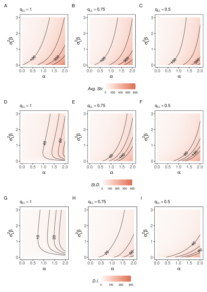
Fig. A.1: Strength Distribution of an MS Poisson LS model: Contour plots of the expected value (Top Panels), standard deviation (Middle Panels), and dispersion index (Bottom Panels) of the Strength Distribution of a two-state MS Poisson LS model for different values of $\alpha$ and $\sigma^{2}_{L}\beta$, and for different transition probabilities $q_{LL}$ and $q_{LH}=1-q_{LL}$. We assume $d=1$, $N=100$, and $\sigma^{2}_{H}\beta=4$.

Appendix B Properties with Simulated Data

As a robustness check, we study the statistical properties of a weighted network generated by the LS model in simulations. We draw the latent coordinates $x_{i}\sim\mathcal{N}(0,\sigma^{2}I_{d})$ for $i=1,\ldots,100$, $d=1$ and $K=1$ and generate the networks weights $Y_{ij}\sim\mathcal{P}oi(\lambda_{ij})$ with intensity parameter $\log\lambda_{ij}=\alpha-\beta||x_{i}-x_{j}||^{2}$.

As is common in network theory, we define the strength of node $i$ as $S_{i}=\sum_{j\neq i}Y_{ij}$. We study the properties of the empirical distribution of $\mathbf{S}=\{S_{1},\ldots,S_{N}\}$. In particular we focus attention on the following statistics: the sample mean $\overline{S}$, the sample standard deviation $SD(S)$, the divergence index $\overline{\mathfrak{D}}(S)$ and the clustering coefficient $CC$ as defined in Barrat et al., (2004).

Figures B.1 and B.2 report the sensitivity analysis for the aforementioned statistics as $\alpha$ and $\sigma^{2}$ vary. In this simulation we assume $\beta=1$. Notice how the theoretical quantities obtained in Appendix A (dashed lines) match with empirical quantities (solid lines).

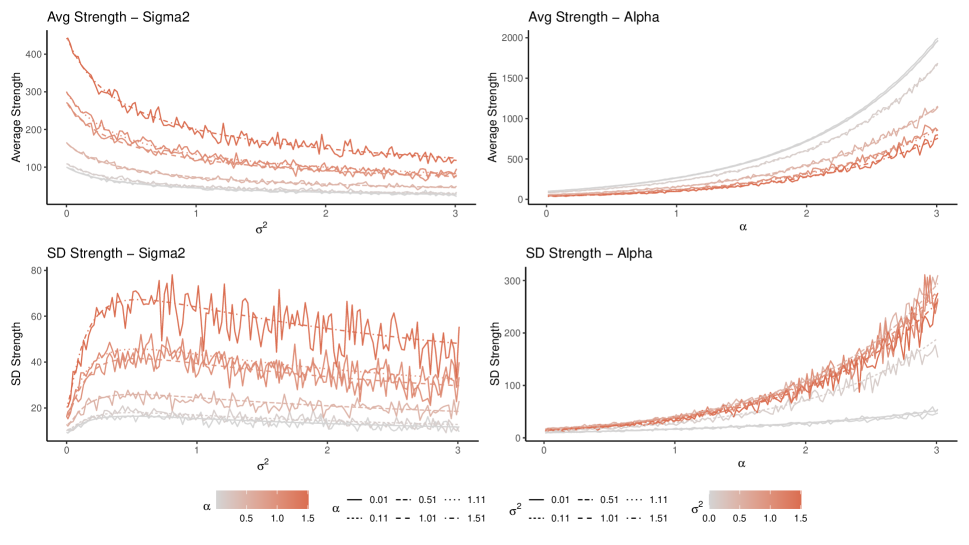
Fig. B.1: Simulation Result - 1

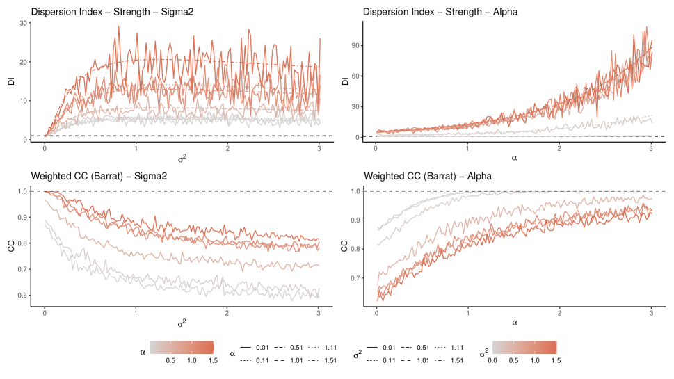
Fig. B.2: Simulation Result - 2

Appendix C Details of the prior and MCMC sampler

The joint likelihood function $f(\mathbf{Y},\bm{\ell}|\bm{\theta})$ is written assuming cross-country independence as the product of the country-specific likelihoods for $r\in 1,\ldots,R$:

$$f(\mathbf{Y}_{r},\bm{\ell}_{r}|\bm{\theta}_{r})=\sum_{\mathbf{s}_{r}\in\{1,\ldots,K_{r}\}^{T_{r}}}\prod_{t=1}^{T_{r}}\prod_{i=1}^{N_{r}}\left(f_{B}(\ell_{irt}|s_{rt},\bm{\theta}_{r})\prod_{j=i+1}^{N_{r}}f_{P}(Y_{ijrt}|s_{rt},\bm{\theta}_{r})\right)h(s_{rt}|s_{rt-1}),$$

where $f_{P}(Y_{ijrt}|s_{rt},\bm{\theta}_{r})$ is the density of the Poisson distribution with dynamic intensity given in (1), $f_{B}(\ell_{irt}|s_{rt},\bm{\theta}_{r})$ the density of the Beta distribution given in (3) and

$$h(s_{rt}|s_{rt-1})=\prod_{l=1}^{K_{r}}\prod_{k=1}^{K_{r}}q_{lkr}^{\mathbb{I}(s_{rt-1}=l)\mathbb{I}(s_{rt}=k)},$$

the hidden Markov chain transition distribution. The joint posterior distribution is not tractable thus a data augmentation has been followed. In addition, given the cross-country independence assumption for both the likelihood and the joint prior, the Gibbs sampler iterates independent chains over the $R$ countries. We report below the prior specification and the full conditional distributions for the components of $\bm{\theta}_{r}$ together with a brief discussion of the sampling method.

C.1 Prior Specification

We take a Bayesian approach to inference and in the prior structure (6), we choose the following prior distributions (as explained in Section 3.2 we fix $\beta_{r}=1$ in our empirical application):

$$\alpha_{ir} \sim\mathcal{N}(0,\sigma^{2}_{\alpha}),\,\bm{\zeta}_{ikr}\sim\mathcal{N}(\bm{0},\sigma^{2}_{kr}I_{d}),\sigma^{2}_{kr}\sim I\mathcal{G}(a_{\sigma^{2}},b_{\sigma^{2}}),$$ (1)

$$\gamma_{0r}\sim\mathcal{N}(0,b_{\gamma_{0}}),\bm{\gamma}_{1r} \sim\mathcal{N}(\bm{0},b_{\gamma_{1}}I_{d}),\,\phi_{r}\sim\mathcal{G}(a_{\phi},b_{\phi}),\,\bm{q}_{lr}\sim\mathcal{D}ir(\omega_{1},\ldots,\omega_{K_{r}}),$$ (2)

where $\mathcal{N}(\bm{\mu},\Sigma)$ denotes a multivariate normal distribution with mean vector $\bm{\mu}$ and variance-covariance matrix $\Sigma$, $\mathcal{G}(a,b)$ denotes the gamma distribution with shape parameter $a$ and precision parameter $b$, with mean $a/b$, $I\mathcal{G}(a,b)$ denotes the inverse-gamma distribution with shape parameter $a$ and scale parameter $b$, with mean $b/(a-1)$ existing for $a>1$ and $\mathcal{D}ir(c_{1},\ldots,c_{K})$ denotes the Dirichlet distribution with parameters $c_{1},\ldots,c_{K}$.

In our implementation of the model with $d=1$ and $K=2$, we have little prior information at our disposal and we opt for the use of relatively vague priors to let the data speak: $\alpha_{ir}\sim\mathcal{N}(0,15^{2})$, ${\zeta}_{ikr}\sim\mathcal{N}(0,\sigma^{2}_{kr})$, $\sigma^{2}_{kr}\sim I\mathcal{G}(0.1,0.1)$, $\gamma_{0r}\sim\mathcal{N}(0,15^{2})$, $\gamma_{1r}\sim\mathcal{N}(0,15^{2})$, $\phi_{r}\sim\mathcal{G}(0.01,0.01)$ and $\bm{q}_{lr}\sim\mathcal{D}ir(2,2)$. Our results are robust to substantial changes in these priors.

C.2 Full conditional distribution of $\alpha_{ir}$

$$p(\alpha_{ir}|\ldots)\propto\pi(\alpha_{ir})f(\mathbf{Y}_{r},\bm{\ell}_{r}|\bm{\theta}_{r})\propto f_{N}(\alpha_{ir};0,\sigma^{2}_{\alpha})\prod_{t=1}^{T_{r}}\prod_{i=1}^{N_{r}}\prod_{j=i+1}^{N_{r}}f_{P}(Y_{ijrt}|\lambda_{ijrt})$$

$$\propto f_{N}(\alpha_{ir};0,\sigma^{2}_{\alpha})\prod_{t=1}^{T_{r}}\prod_{i=1}^{N_{r}}\prod_{j=i+1}^{N_{r}}\lambda_{ijrt}^{Y_{ijrt}}e^{-\lambda_{ijrt}},$$

where $\log\lambda_{ijrt}=\alpha_{ir}+\alpha_{jr}-||\bm{\zeta}_{ir}\bm{\xi}_{rt}-\bm{\zeta}_{jr}\bm{\xi}_{rt}||^{2}$. We sample from $p(\alpha_{ir}|\ldots)$ via Adaptive RW-MH.

C.3 Full conditional distribution of $\phi_{r}$

$$p(\phi_{r}|\ldots)\propto\pi(\phi_{r})f(\mathbf{Y}_{r},\bm{\ell}_{r}|\bm{\theta}_{r})$$

$$\propto\phi_{r}^{a_{\phi}-1}e^{-b_{\phi}\phi_{r}}\prod_{t=1}^{T_{r}}\prod_{i=1}^{N_{r}}\frac{\ell^{a_{irt}-1}_{irt}(1-\ell_{irt})^{b_{irt}-1}}{B(a_{irt},b_{irt})},$$

where $a_{irt}=\varphi(\gamma_{0r}+\gamma_{1r}\bm{\zeta}_{ir}\bm{\xi}_{rt})\phi_{r}$, $b_{irt}=\left(1-\varphi(\gamma_{0r}+\gamma_{1r}\bm{\zeta}_{ir}\bm{\xi}_{rt})\right)\phi_{r}$. We sample from $p(\phi_{r}|\ldots)$ via RW-MH with a truncated Gaussian proposal.

C.4 Full conditional distribution of $\gamma_{0r}$ and $\gamma_{1r}$

$$p(\gamma_{0r},\gamma_{1r}|\ldots)\propto\pi(\gamma_{0r},\gamma_{1r})f(\mathbf{Y}_{r},\bm{\ell}_{r}|\bm{\theta}_{r})$$

$$\propto f_{N}(\gamma_{0r};0,b_{\gamma_{0}})f_{N}(\gamma_{1r};0,b_{\gamma_{1}})\prod_{t=1}^{T_{r}}\prod_{i=1}^{N_{r}}\frac{\ell^{a_{irt}-1}_{irt}(1-\ell_{irt})^{b_{irt}-1}}{B(a_{irt},b_{irt})},$$

where $a_{irt}=\varphi(\gamma_{0r}+\gamma_{1r}\bm{\zeta}_{ir}\bm{\xi}_{rt})\phi_{r}$, $b_{irt}=(1-\varphi(\gamma_{0r}+\gamma_{1r}\bm{\zeta}_{ir}\bm{\xi}_{rt}))\phi_{r}$. We sample from $p(\gamma_{0r},\gamma_{1r}|\ldots)$ via RW-MH.

C.5 Full conditional distribution of $\zeta_{ikr}$

$$p(\zeta_{ikr}|\ldots)\propto\pi(\zeta_{ikr}|\sigma_{kr}^{2})f(\mathbf{Y}_{r},\bm{\ell}_{r}|\bm{\theta}_{r})$$

$$\propto f_{N}(\zeta_{ikr};0,\sigma^{2}_{kr})\prod_{t\in\mathcal{T}_{kr}}\frac{\ell^{a_{irt}-1}_{irt}(1-\ell_{irt})^{b_{irt}-1}}{B(a_{irt},b_{irt})}\prod_{j\in\mathcal{S}_{r}^{-i}}\lambda_{ijrt}^{Y_{ijrt}}e^{-\lambda_{ijrt}},$$

where $\mathcal{T}_{kr}=\{t:\xi_{krt}=1\}$, $\mathcal{S}_{r}^{-i}=\{j\in 1,\ldots N_{r}:j\neq i\}$, $\log\lambda_{ijrt}=\alpha_{ir}+\alpha_{jr}-||\bm{\zeta}_{ir}\bm{\xi}_{rt}-\bm{\zeta}_{jr}\bm{\xi}_{rt}||^{2}$, $a_{irt}=\varphi(\gamma_{0r}+\gamma_{1r}\bm{\zeta}_{ir}\bm{\xi}_{rt})\phi_{r}$, $b_{irt}=(1-\varphi(\gamma_{0r}+\gamma_{1r}\bm{\zeta}_{ir}\bm{\xi}_{rt}))\phi_{r}$. We sample from $p(\zeta_{ikr}|\ldots)$ via Adaptive RW-MH (see Subsection C.8).

C.6 Full conditional distribution of $\sigma^{2}_{kr}$

$$p(\sigma^{2}_{kr}|\bm{\zeta}_{kr},\bm{\xi}_{r})\propto\pi(\sigma^{2}_{kr})\pi(\bm{\zeta}_{kr}|\sigma^{2}_{kr},\bm{\xi}_{r})$$

$$\propto(1/\sigma^{2}_{kr})^{a_{\sigma^{2}}+1}e^{-b_{\sigma^{2}}\frac{1}{\sigma^{2}_{kr}}}\prod_{i=1}^{N_{r}}\left(1/\sigma_{kr}^{2}\right)^{\frac{1}{2}}e^{-\frac{1}{2\sigma^{2}_{kr}}\bm{\zeta}_{ikr}^{2}}$$

$$\propto(1/\sigma^{2}_{kr})^{a_{\sigma^{2}}+1}e^{-b_{\sigma^{2}}\frac{1}{\sigma^{2}_{kr}}}\left(1/\sigma_{kr}^{2}\right)^{\frac{N_{r}}{2}}e^{-\frac{1}{2\sigma^{2}_{kr}}\sum_{i=1}^{N_{r}}\bm{\zeta}_{ikr}^{2}}$$

$$\propto(1/\sigma^{2}_{kr})^{a_{\sigma^{2}}+\frac{N_{r}}{2}+1}e^{-\left(b_{\sigma^{2}}+\frac{\sum_{i=1}^{N_{r}}\bm{\zeta}_{ikr}^{2}}{2}\right)\frac{1}{\sigma^{2}_{kr}}},$$

which is the density function of an $I\mathcal{G}(a^{*}_{\sigma^{2}kr},b^{*}_{\sigma^{2}kr})$ distribution where $a^{*}_{\sigma^{2}kr}=a_{\sigma^{2}}+\frac{N_{r}}{2}$ and $b^{*}_{\sigma^{2}kr}=b_{\sigma^{2}}+\frac{\sum_{i=1}^{N_{r}}\zeta^{2}_{ikr}}{2}$.

C.7 Full conditional distribution of $\bm{q}_{lr}$

$$p(\bm{q}_{lr}|\bm{\xi})\propto\left(\prod_{t=1}^{T_{r}}\prod_{k=1}^{K_{r}}q_{lkr}^{\xi_{lrt-1}\xi_{krt}}\right)\left(\prod_{k=1}^{K_{r}}q^{\omega_{k}-1}_{lk}\right)$$

$$\propto\prod_{k=1}^{K_{r}}q_{lk}^{\sum_{t=1}^{T_{r}}(\xi_{lrt-1}\xi_{krt})+\omega_{k}-1},$$

which is the density function of a Dirichlet distribution with parameters $\bar{\omega}_{1r},\ldots,\bar{\omega}_{Kr}$ where $\bar{\omega}_{kr}=\sum_{t=1}^{T_{r}}(\xi_{lrt-1}\xi_{krt})+\omega_{k}-1$.

C.8 Adaptive MCMC

Sampling from the full conditional of $\bm{\alpha}_{r}$ and $\bm{\zeta}_{kr}$ is obtained via Adaptive MH algorithm with global adaptive scaling proposed in Andrieu and Thoms, (2008). Adaptive MH generates samples from the distribution of $\bm{\theta}$ by iterating the following steps:

1. Starting values for the parameter of interest $\bm{\theta}_{0}$ and for $\bm{\mu}_{0}$ and $\bm{\Sigma}_{0}$ are chosen.

2. For each iteration $h$, given $\bm{\theta}_{h}$, $\bm{\mu}_{h}$, $\bm{\Sigma}_{h}$ and $\delta_{h}$:

   1. $\tilde{\bm{\theta}}_{h}\sim f_{N}(\bm{\theta}_{h-1};\delta_{h-1}\bm{\Sigma}_{h-1})$ is sampled and $\bm{\theta}_{h}=\tilde{\bm{\theta}}_{h}$ with probability $\alpha(\bm{\theta}_{h-1},\tilde{\bm{\theta}}_{h})$, otherwise $\tilde{\bm{\theta}}_{h}=\bm{\theta}_{h-1}$;

   2. Update $\log(\delta_{h})=\log(\delta_{h-1})+\gamma_{h}[\alpha(\bm{\theta}_{h-1},\tilde{\bm{\theta}}_{h})-\alpha^{*}]$;

   3. Update $\bm{\mu}_{h}=\bm{\mu}_{h-1}+\gamma_{h}(\bm{\theta}_{h}-\bm{\mu}_{h-1})$;

   4. Update $\bm{\Sigma}_{h}=\bm{\Sigma}_{h-1}+\gamma_{h}[(\bm{\theta}_{h}-\bm{\mu}_{h-1})(\bm{\theta}_{h}-\bm{\mu}_{h-1})^{\prime}-\bm{\Sigma}_{h-1}]$;

   where $\gamma_{h}=\frac{1}{h^{\psi}}$ for $\psi\in(0,1)$ and $\alpha^{*}$ is a target acceptance rate, here chosen to be 25%.

Appendix D MCMC Properties for the Simulated Data

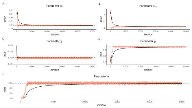
Fig. D.1: Simulation Output: Trace plots for the parameters $\alpha_{1}$ (Panel A), $\alpha_{11}$ (Panel B), $\gamma_{0}$ (Panel C), $\gamma_{1}$ (Panel D) and $\phi$ (Panel E). The solid black line represents the cumulative average while the dashed black line represents the true parameter in the simulation.

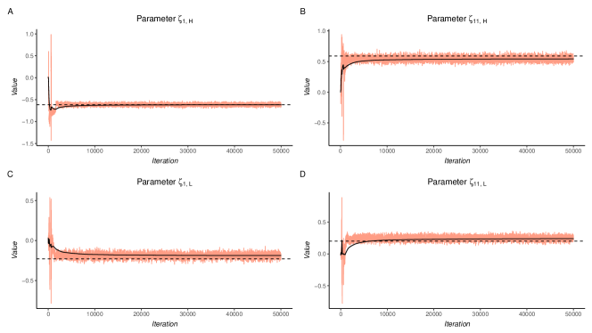
Fig. D.2: Simulation Output: Trace plots for the latent leaning for outlet $1$ – $\zeta_{1,L}$ (Panel A), $\zeta_{1,H}$ (Panel B) – an for outlet $11$ – $\zeta_{11,L}$ (Panel C), $\zeta_{11,H}$ (Panel D). The solid black line represents the cumulative average while the dashed black line represents the true parameter in the simulation.

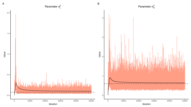
Fig. D.3: Simulation Output: Trace plots for the parameters $\sigma^{2}_{L}$ and $\sigma^{2}_{H}$. The solid black line represents the cumulative average while the dashed black line represents the true parameter in the simulation.

Table D.1: Simulated data: Auto-correlation (ACF) at lag 1, 10, 30, Acceptance Rate, Effective Sample Size over the number of draws (ESS) and Convergence Diagnostic p-value (CD) as defined in Geweke, (1992) for the MCMC sampling of $\bar{\alpha}$, $\gamma_{0}$, $\gamma_{1}$, $\phi$, $\bar{\zeta}_{L}$, $\bar{\zeta}_{H}$ respectively on the raw series, on the series collected after burn-in, and on the series applying burn-in and thinning.

Raw Series (50,000 obs.)
Parameter	$\bar{\alpha}_{i}$	$\gamma_{0}$	$\gamma_{1}$	$\phi$	$\bar{\zeta}_{L}$	$\bar{\zeta}_{H}$
ACF(1)	0.996	0.788	0.997	0.980	0.924	0.956
ACF(10)	0.972	0.190	0.978	0.925	0.713	0.803
ACF(30)	0.930	0.009	0.947	0.911	0.487	0.641
Acc.	25%	26%	26%	21%	25%	25%
ESS	0%	8%	0%	0%	2%	1%
CD p-val	0.050	0.175	0.000	0.000	0.109	0.142
With Burn-in (20,000 obs.)
Parameter	$\bar{\alpha}_{i}$	$\gamma_{0}$	$\gamma_{1}$	$\phi$	$\bar{\zeta}_{L}$	$\bar{\zeta}_{H}$
ACF(1)	0.891	0.730	0.898	0.750	0.849	0.766
ACF(10)	0.529	0.034	0.398	0.067	0.374	0.149
ACF(30)	0.318	-0.017	0.145	-0.011	0.174	0.048
Acc.	25%	25%	25%	22%	25%	25%
ESS	3%	16%	4%	14%	6%	10%
CD p-val	0.213	0.399	0.040	0.146	0.300	0.256
With Burn-in and Thinning every 10 (2000 obs.)
Parameter	$\bar{\alpha}_{i}$	$\gamma_{0}$	$\gamma_{1}$	$\phi$	$\bar{\zeta}_{L}$	$\bar{\zeta}_{H}$
ACF(1)	0.527	0.017	0.401	0.040	0.367	0.149
ACF(10)	0.135	-0.005	0.054	0.028	0.057	0.011
ACF(30)	0.022	0.022	0.003	0.004	0.005	0.008
Acc.	-	-	-	-	-	-
ESS	23%	100%	35%	93%	44%	66%
CD p-val	0.209	0.402	0.033	0.013	0.275	0.259

Appendix E Model Selection

We compute DIC to compare models as in Gelman et al., (2014): $DIC_{r}(\mathcal{M}_{r})=-2\overline{\log f}(\mathbf{Y}_{r},\bm{\ell}_{r}|\bm{\theta},\mathcal{M}_{r})+p_{D}$, where $\overline{\log f}(\mathbf{Y}_{r},\bm{\ell}_{r}|\bm{\theta},\mathcal{M}_{r})=(1/H)\sum_{h=1}^{H}\log f(\mathbf{Y}_{r},\bm{\ell}_{r}|\bm{\theta}^{h}_{r},\mathcal{M}_{r})$ is the sample average of the loglikelihood computed at each iteration $h$ of model $\mathcal{M}$ while $p_{D}=2Var\left(\log f(\mathbf{Y}_{r},\bm{\ell}_{r}|\bm{\theta}^{1:H}_{r},\mathcal{M}_{r})\right)$. We also compute the Log Pointwise Predictive Density (lppd) as in Gelman et al., (2014): $lppd_{r}(\mathcal{M}_{r})=\sum_{i>j,t}\log\left(\frac{1}{H}\sum_{h=1}^{H}f_{P}\left(Y_{ijrt}\mid\bm{\theta}_{r}^{h},\mathcal{M}_{r}\right)\right)$.

Table E.1: Model Selection: DIC-score components for the three nested models considered for each country.

Model	France	Germany	Italy	Spain
	$\overline{\log f}_{P}(\mathbf{Y}_{r}|\bm{\theta}_{r},\mathbf{s}_{r},\mathcal{M})\times 10^{-6}$
$\mathcal{M}_{1}$	$\mathbf{-2.2796}$	$\mathbf{-1.2198}$	-1.6789	$\mathbf{-2.3365}$
$\mathcal{M}_{2}$	$-2.2796$	-1.2198	$\mathbf{-1.6788}$	-2.3491
$\mathcal{M}_{3}$	-2.3602	-1.2706	-1.7664	-2.4536
	$\overline{\log f}(\mathbf{Y}_{r},\bm{\ell}_{r}|\bm{\theta}_{r},\mathbf{s}_{r},\mathcal{M})\times 10^{-6}$
$\mathcal{M}_{1}$	$\mathbf{-2.2347}$	$\mathbf{-1.1834}$	$\mathbf{-1.6524}$	$\mathbf{-2.3069}$
$\mathcal{M}_{2}$	-2.2348	-1.1834	-1.6532	-2.3194
$\mathcal{M}_{3}$	-2.3153	-1.2342	-1.7397	-2.4240

Appendix F Details of the Observable Media Slant Index

To construct an observable proxy for media slant we rely on the methodology proposed by Gentzkow and Shapiro, (2010) and extended to online textual data by Garz et al., (2020). Textual processing is carried out with the use of the R package quanteda. The underlying intuition is that of computing the distance between the language used by news outlets in their posts and the language used by political parties. To do so we compose two corpora of textual data: the Parties Corpus consisting of the textual content of the posts published by the major parties in the years 2015-2016 on their Facebook wall, the Outlets Corpus consisting of the same information related to the posts published by the Italian news outlets considered in this work.

On both corpora, textual pre-processing is carried out (lower case transformation, punctuation removal, stopwords removal and n-gram tokenization) and tokens not present in the Outlets corpus are filtered out from the Parties Corpus. By means of the TF-IDF score applied on the Parties Corpus, we retrieve the top 100 tokens with highest TF-IDF score for each party. We proceed assessing the cosine similarity between the vector of tokens $\mathbf{x}_{t,o}$ obtained from the set of posts published by outlet $o$ at time $t$ and the set of tokens $\mathbf{y}_{p}$ characteristic of each party $p$.

$$sim_{pot}=\frac{\sum_{k=1}^{K}x_{kot}y_{kp}}{\sqrt{\sum_{k=1}^{K}x^{2}_{kot}}\sqrt{\sum_{k=1}^{K}y^{2}_{kp}}}$$

To take into account the fact that the style of posting adopted by some parties is closer to the one of news outlets and vice-versa, Garz et al., (2020) suggest regressing the similarity on a constant and both outlet and party fixed-effects to extract the residuals $\epsilon_{pot}$, which can be interpreted as a proxy of unexplained similarity. Finally the media slant for outlet $o$ at time $t$ is computed as:

$$slant_{ot}=\sum_{p=1}^{P}\epsilon_{pot}score_{p}$$

where $score_{p}$ is the political leaning assigned to party $p$ by the 2014 Chapel Hill Experts Survey classification provided in Polk et al., (2017), see Fig. F.1.

Figure F.2 reports the average media slant for the available set of news outlets for France, Germany, Italy, and Spain, trough the whole time lapse.

Fig. F.1: Ideology of Political Parties: The index is computed according to the 2014 Chapel Hill Experts Survey (Polk et al.,, 2017).

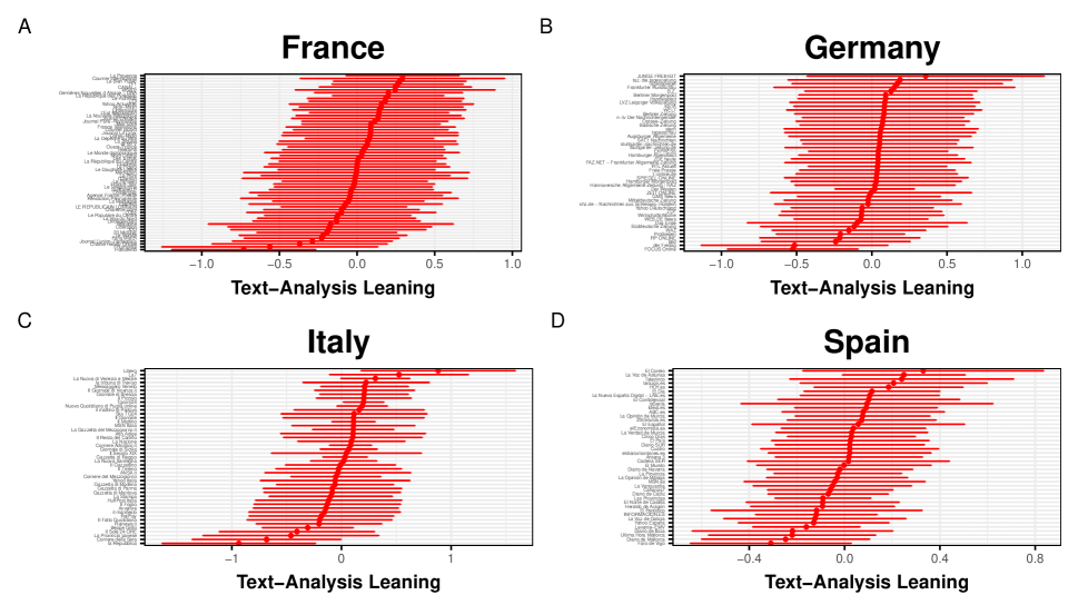
Fig. F.2: Media Slant of News Outlets: The index is computed following the methodology proposed by Gentzkow and Shapiro, (2010) and Garz et al., (2020). Full dots represent the average leaning and error bars represent the $\mu\pm\sigma$ interval over the time-lapse.

Appendix G Identifiers and List of Removed Outlets

The table below lists the news outlets used as identifiers of the political orientation.

Table G.1: Identifiers: Set of outlets used to identify the political orientation of the news outlets. The column sign reports the assumed political orientation: either < (left) or > (right). The column PEW score reports the estimated leaning as per Mitchell et al.,, 2018.

News Outlet	Country	Assumed Media Bias	Sign	PEW score (0-6)
l’Humanité	France	Left	<0	NA
Bild	Germany	Center-Right	>0	3.1
Libero	Italy	Center-Right	>0	3.6
ABC	Spain	Center-Right	>0	3.3

A few news outlets were removed in the dynamic analysis because of their prolonged inactivity, i.e. 15 days without any comment. They are DE: Der Westen, GMX News, WEB.DE, News ZDF, FR: Charlie Hebdo Officiel, France Télévisions, Franceinfo, LCI, Révolution Permanente, IT: La Gazzetta del Mezzogiorno.it, MSN Italia, SP: La Voz de Asturias, Yahoo España.

Appendix H Controlling for Exposure

Here we discuss the inclusion of an additional variable, $TotCom_{rt}$, accounting for the exposure to the total number of comments at time $t$. This is to compare polarisation across periods with different engagement levels. To maintain parameter interpretation, we add to the log-intensity the de-meaned logarithm of the total number of comments, $\log TotCom_{rt}$:

$$\log\lambda_{ijrt}=\alpha_{ir}+\alpha_{jr}+\delta\log TotCom_{rt}-\beta_{r}||x_{irt}-x_{jrt}||^{2}.$$

We run our modified LS model for the Italian data. Figure H.1 reports the posterior estimates of the latent space and states through time when we include this control. Panel A reports the latent space of Italian news outlets in the two states. State identification is not trivial anymore. In fact, we notice heterogeneous behavior between local and national outlets. We achieve state identification by considering the average distance computed across national news outlets (triangles), as they involve a larger number of commenters. Panel B reports the latent states through time. The states are coherent with those found in Sec. 4. Figure H.2 reports the marginal posteriors draws for the parameters $\delta$, $\gamma_{0r}$, $\gamma_{1r}$ and $\phi_{r}$. The sign of the parameter $\delta$ is as expected. Higher comments overall in the network implies also a higher number of comments in common between the pairs of pages.

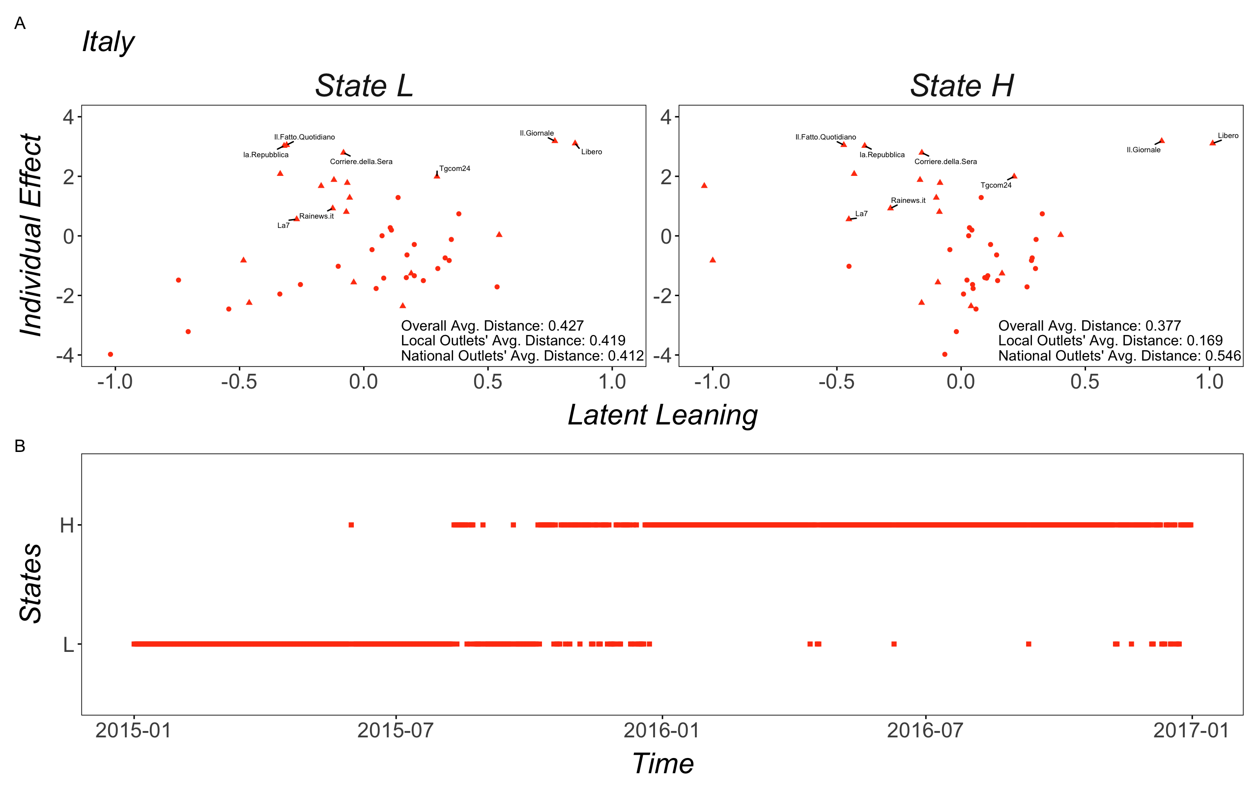
Fig. H.1: Posterior Mean Latent Space and States with Exposure Control: Panel A reports the latent space of Italian news outlets in the two states. State identification is achieved considering the average distance computed across national news outlets (triangles). Panel B reports the latent states through time. The states are coherent with those found in Sec. 4.

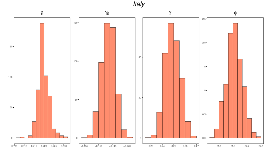
Fig. H.2: Marginal Posterior Distributions with Exposure Control: Histograms for the MCMC draws for the parameters $\delta$, $\gamma_{0r}$, $\gamma_{1r}$ and $\phi_{r}$ for Italy.

Appendix I Further Results for the Facebook Data

Figure I.1 allows us to assess the agreement between latent coordinates and the PEW Research index for $d=2$. The figure highlights how one latent dimension retains the agreement with the PEW Research index even in a higher dimensional space.

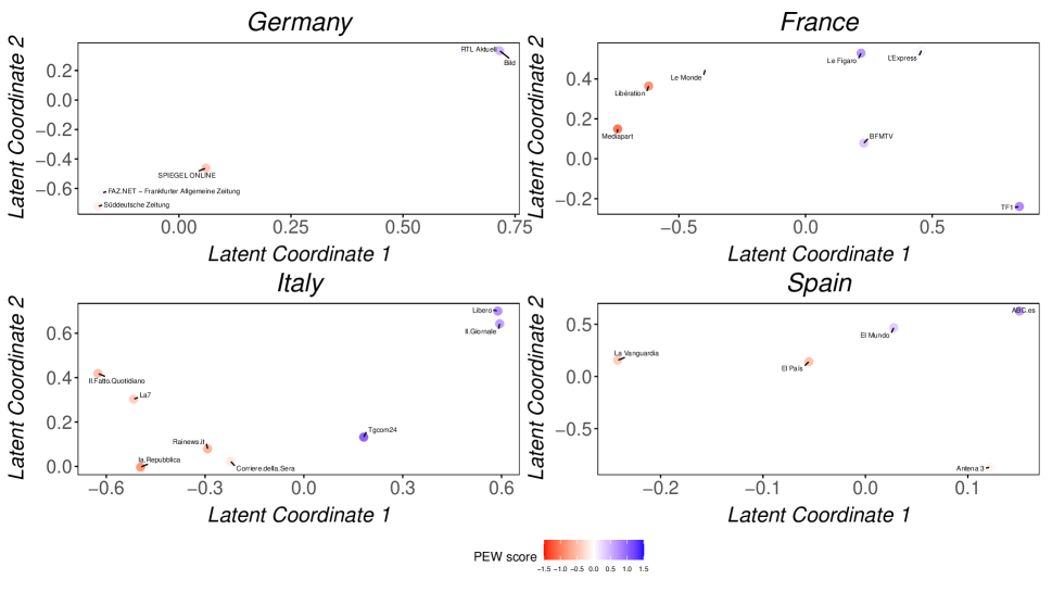
Fig. I.1: Robustness - Higher dimensional space - Static Analysis: Latent-space representation of the news outlets considered by PEW Research for $d=2$. News outlets are color-coded from left (red) to right (blue) according to the centered PEW Research Index. The latent dimension retains the agreement with the PEW Research index even when a higher dimensional space is considered.

Figure I.2 presents the posterior distributions of the parameters of the static LS model for the Facebook data.

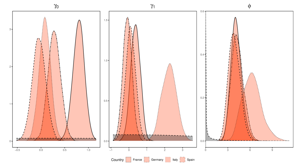
Fig. I.2: Marginal Posteriors - Static Analysis: Kernel density estimates of the posterior for the parameters $\gamma_{0r}$, $\gamma_{1r}$ and $\phi_{r}$ for France, Germany, Italy and Spain with prior pdfs indicated by grey dashed lines.

France	Germany
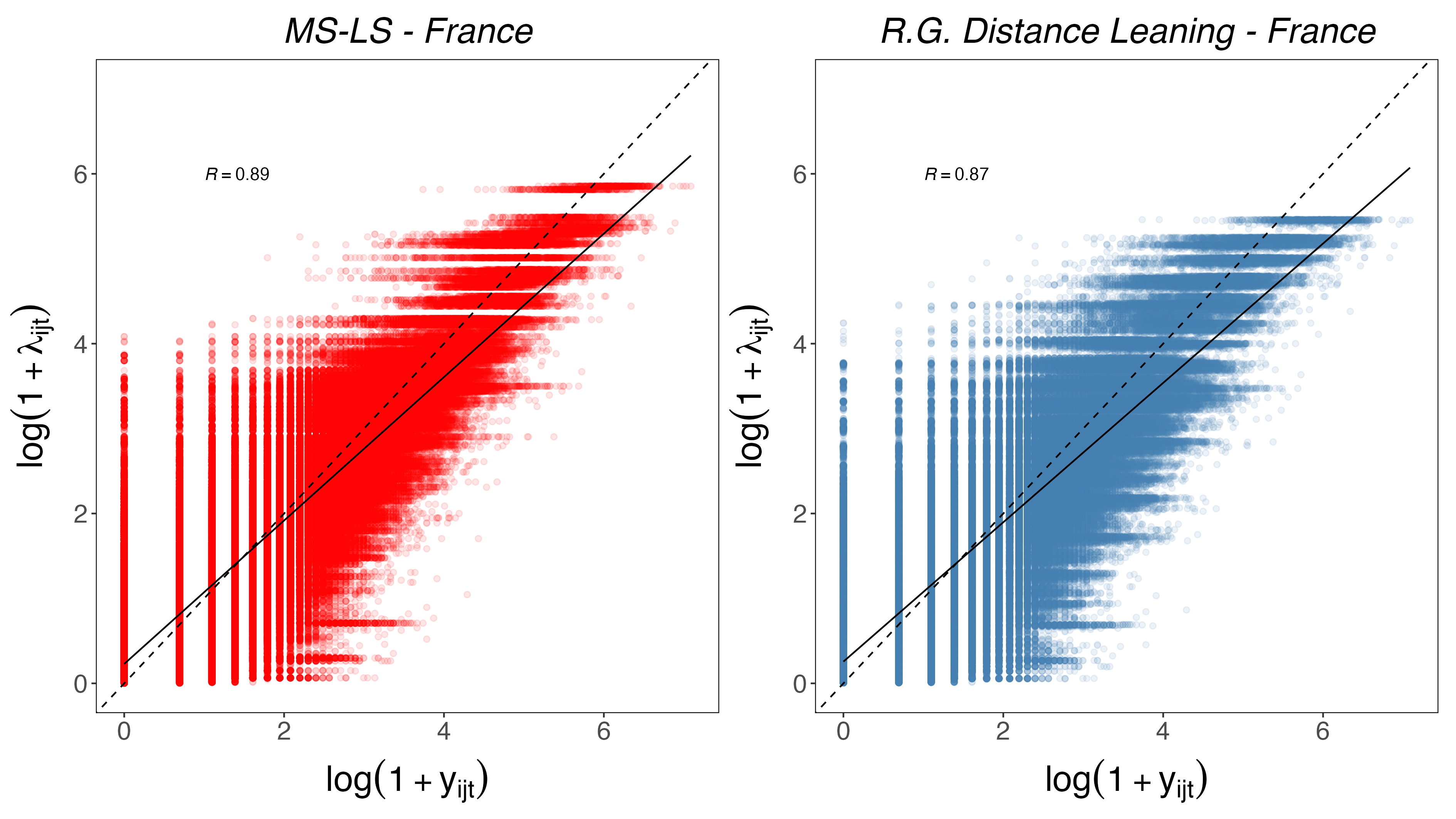
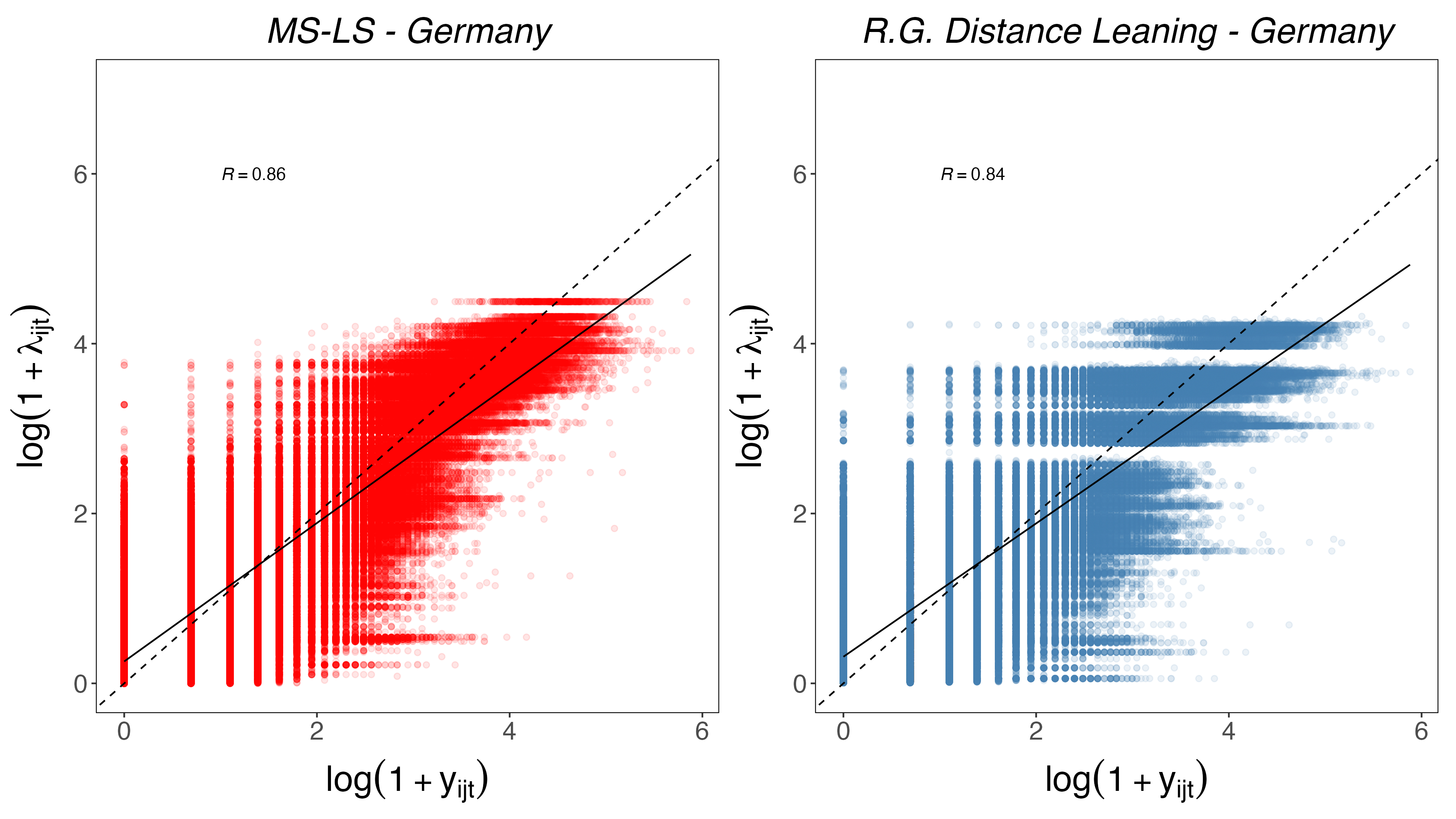
Italy	Spain

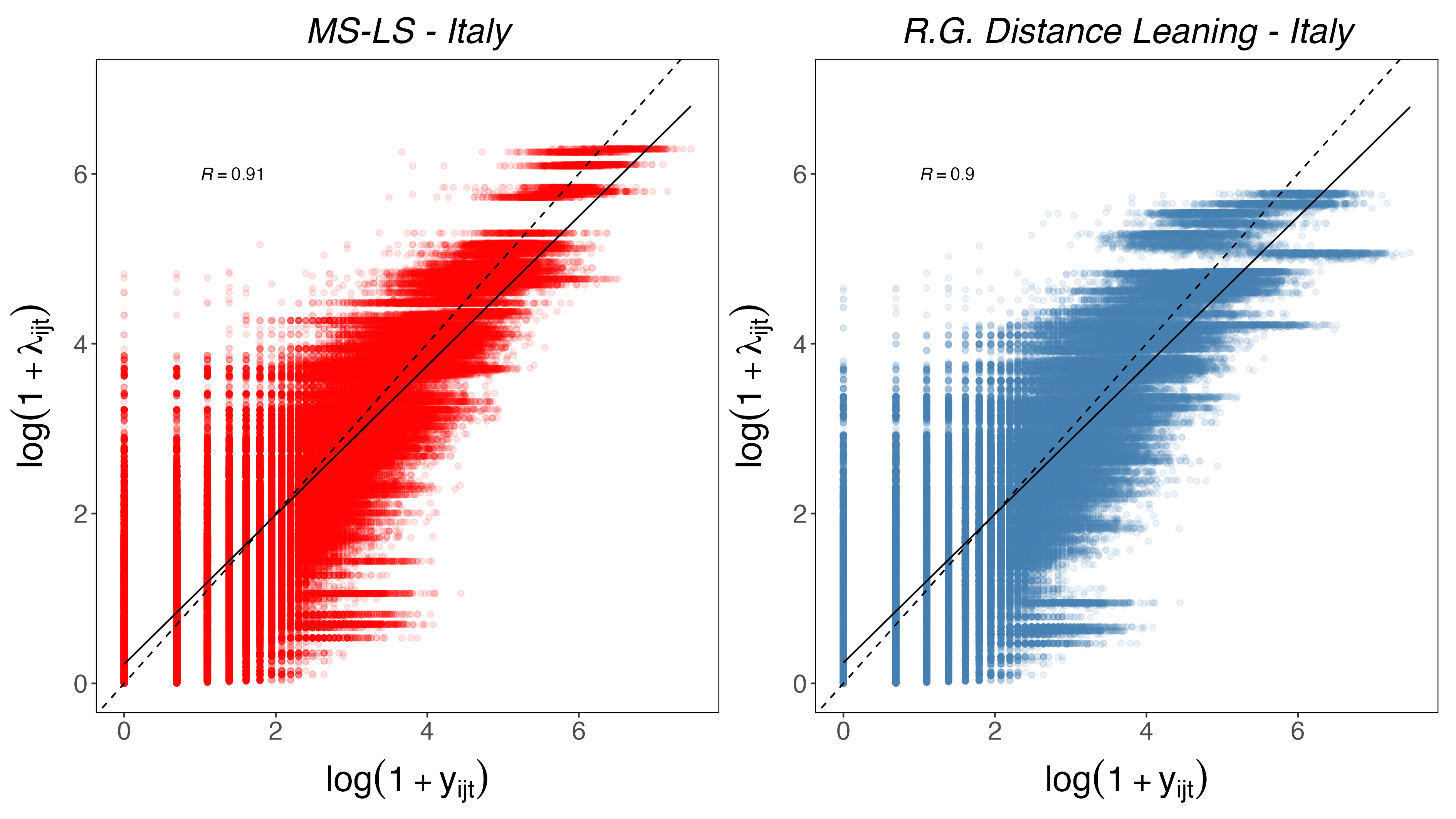
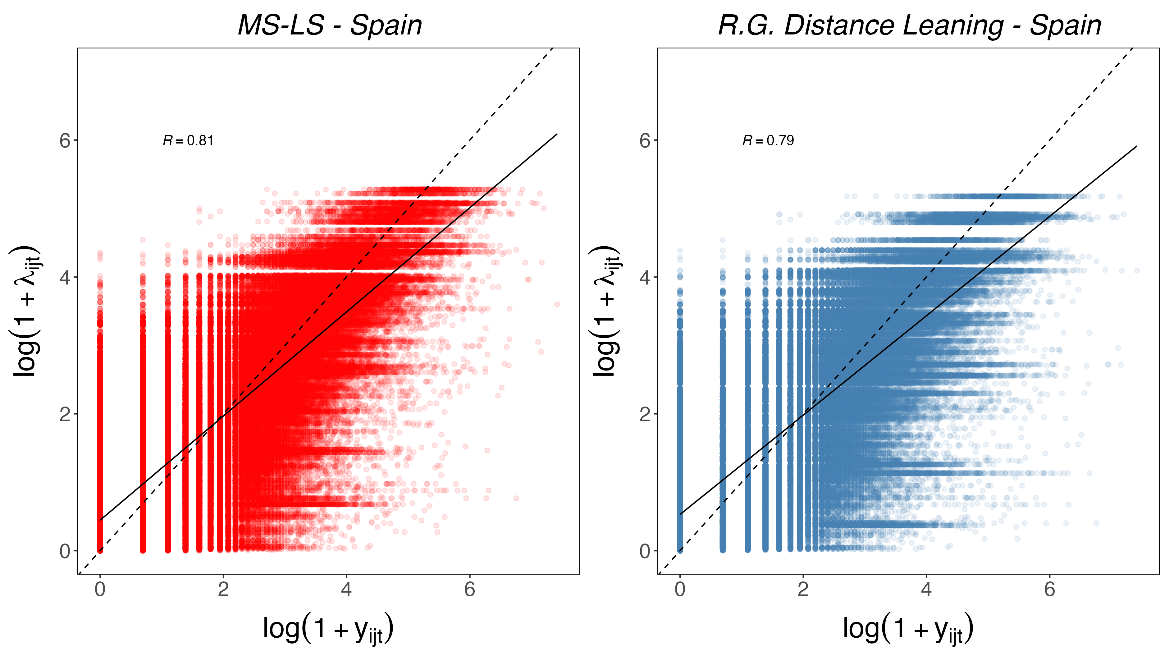
Fig. I.3: Predictive-Check Comparison: Scatter plot of $y_{ijrt}$ and the posterior $\lambda_{ijt}$ for the MS-LS model (left panels) and for the R.G. model with the observed-leaning distance covariate in log scales. We also plot the 45-degree line (dashed) and the set of regression lines for each iteration (solid lines, very close to each other)

Appendix J Data and Scripts Repository

Data and Scripts are stored in the following Repository: https://github.com/BayesianEcon/Dyn-MS-LS-Media. Refer to the README file in the repository for a complete description of each file.

J.1 Data

The data entirely covers 729 days from "2015-01-01" to "2016-12-31". The number of news outlets included in each dataset is the following: Germany 47 news outlets, France 62, Italy 45 and Spain 43.

Network Dataset:

Data set used in the illustration of the MS-LS Network Model in Section 4. The data set is an edge-list representation of the media networks where columns "i" and "j" refer to the nodes, column "t" refers to the day and column "w" refers to the number of unique Facebook commenters in common between "i" and "j" at time "t". The static-version of the Network Dataset of each country is contained within the file ("Data_Env_single_(country).RData"), while the dynamic version is in the file ("DataEnv_(country)_all.RData").

Slant-Index Dataset:

Data set used in the illustration of the MS-LS Network Model in Section 4. Refer to Appendix F and the README file for an illustration of how the index has been obtained. The data set represents a nodal feature of the media networks where column "i" refers to the nodes, column "t" refers to the day and column "leaning" refers to the Slant Index.

The static version of the Slant-Index Dataset of each country is contained within the file ("Data_Env_single_(country).RData"), while the dynamic version is included in the file ("DataEnv_(country)_all.RData").

J.2 Scripts

We report here a brief description of the main scripts used to estimate the Bayesian MS-LS network model on the datasets studied in the main paper (Sections 3 and 4) and the supplementary material. Our MCMC algorithm is entirely implemented in C++, enabling faster execution speed compared to interpreted languages like R or Python. However, we still rely on R for data manipulation and plotting. The smooth integration of the two languages has been made possible through the utilization of the Rcpp package, which offers a convenient interface for invoking C++ scripts within R. Refer to the README.txt file in the repository for a complete description of each script.

Simulation_02_results.R:

Estimates the MS-LS model on the simulated network dataset.
Running time $\sim$ 12 mins (50,000 iterations, Apple M2, 8 GB Memory)

Static_01_Results_(country).R:

Estimates the MS-LS model on the static network dataset.
Running time $\sim$ 45 mins. (15,000 iterations, Apple M2, 8 GB Memory)

Dynamic_01_Results_(country).R:

Estimates the MS-LS model on the dynamic network dataset.
Running time > 20 hrs. (35,000 iterations, Apple M2, 8 GB Memory)

MS_LS_FE.cpp:

The script contains the function to generate MCMC draws for the dynamic Bayesian MS-LS network model.

References

- Anderson and McLaren, (2012) Anderson, S. P. and McLaren, J. (2012). Media Mergers and Media Bias with Rational Consumers. Journal of the European Economic Association, 10(4):831–859.
- Andrieu and Thoms, (2008) Andrieu, C. and Thoms, J. (2008). A Tutorial on Adaptive MCMC. Statistics and Computing, 18(4):343–373.
- Barberá, (2015) Barberá, P. (2015). Birds of the Same Feather Tweet Together: Bayesian Ideal Point Estimation using Twitter Data. Political Analysis, 23(1):76–91.
- Barrat et al., (2004) Barrat, A., Barthelemy, M., Pastor-Satorras, R., and Vespignani, A. (2004). The Architecture of Complex Weighted Networks. Proceedings of the National Academy of Sciences, 101(11):3747–3752.
- Chen et al., (2023) Chen, C. Y.-H., Okhrin, Y., and Wang, T. (2023). Monitoring Network Changes in Social Media. Journal of Business & Economic Statistics, page doi: 10.1080/07350015.2021.2016425.
- Cinelli et al., (2021) Cinelli, M., Morales, G. D. F., Galeazzi, A., Quattrociocchi, W., and Starnini, M. (2021). The Echo Chamber Effect on Social Media. Proceedings of the National Academy of Sciences, 118(9):e2023301118.
- CrowdTangle Team, (2022) CrowdTangle Team (2022). CrowdTangle. Menlo Park, CA: Meta.
- Dandekar et al., (2013) Dandekar, P., Goel, A., and Lee, D. T. (2013). Biased Assimilation, Homophily, and the Dynamics of Polarization. Proceedings of the National Academy of Sciences, 110(15):5791–5796.
- D’Angelo et al., (2019) D’Angelo, S., Murphy, T. B., and Alfò, M. (2019). Latent Space Modelling of Multidimensional Networks with Application to the Exchange of Votes in Eurovision Song Contest. The Annals of Applied Statistics, 13(2):900 – 930.
- De Nicola et al., (2023) De Nicola, G., Tuekam Mambou, V. H., and Kauermann, G. (2023). COVID-19 and Social Media: Beyond Polarization. PNAS Nexus, 2(8):pgad246.
- Esteban and Ray, (1994) Esteban, J.-M. and Ray, D. (1994). On the Measurement of Polarization. Econometrica, 62(4):819–851.
- Friel et al., (2016) Friel, N., Rastelli, R., Wyse, J., and Raftery, A. E. (2016). Interlocking Directorates in Irish Companies using a Latent Space Model for Bipartite Networks. Proceedings of the National Academy of Sciences, 113(24):6629–6634.
- Frühwirth-Schnatter, (2006) Frühwirth-Schnatter, S. (2006). Finite Mixture and Markov Switching Models. Springer Science & Business Media.
- Garimella et al., (2018) Garimella, K., Morales, G. D. F., Gionis, A., and Mathioudakis, M. (2018). Quantifying Controversy on Social Media. ACM Transactions on Social Computing, 1(1):1–27.
- Garz et al., (2020) Garz, M., Sörensen, J., and Stone, D. F. (2020). Partisan Selective Engagement: Evidence from Facebook. Journal of Economic Behavior & Organization, 177:91–108.
- Gelman et al., (2014) Gelman, A., Hwang, J., and Vehtari, A. (2014). Understanding Predictive Information Criteria for Bayesian Models. Statistics and Computing, 24(6):997–1016.
- Gentzkow and Shapiro, (2010) Gentzkow, M. and Shapiro, J. M. (2010). What Drives Media Slant? Evidence from US Daily Newspapers. Econometrica, 78(1):35–71.
- Gentzkow et al., (2015) Gentzkow, M., Shapiro, J. M., and Stone, D. F. (2015). Media Bias in the Marketplace: Theory. In Handbook of Media Economics, volume 1, pages 623–645. Elsevier.
- Geweke, (1992) Geweke, J. F. (1992). Evaluating the Accuracy of Sampling-based Approaches to the Calculation of Posterior Moments. In Berger, J., Bernardo, J., Dawid, A., and Smith, A., editors, Bayesian Statistics 4, pages 169–194. Oxford: Oxford University Press.
- Gollini and Murphy, (2016) Gollini, I. and Murphy, T. B. (2016). Joint Modeling of Multiple Network Views. Journal of Computational and Graphical Statistics, 25(1):246–265.
- Handcock et al., (2007) Handcock, M. S., Raftery, A. E., and Tantrum, J. M. (2007). Model-based Clustering for Social Networks. Journal of the Royal Statistical Society: Series A, 170(2):301–354.
- Hanusch and Nölleke, (2019) Hanusch, F. and Nölleke, D. (2019). Journalistic Homophily on Social Media: Exploring Journalists’ Interactions with Each Other on Twitter. Digital Journalism, 7(1):22–44.
- Hoff et al., (2002) Hoff, P. D., Raftery, A. E., and Handcock, M. S. (2002). Latent Space Approaches to Social Network Analysis. Journal of the American Statistical Association, 97(460):1090–1098.
- Iyengar et al., (2012) Iyengar, S., Sood, G., and Lelkes, Y. (2012). Affect, Not Ideology: A Social Identity Perspective on Polarization. Public opinion quarterly, 76(3):405–431.
- Kim et al., (2018) Kim, B., Lee, K. H., Xue, L., and Niu, X. (2018). A Review of Dynamic Network Models with Latent Variables. Statistics Surveys, 12:105.
- Kubin and von Sikorski, (2021) Kubin, E. and von Sikorski, C. (2021). The Role of (Social) Media in Political Polarization: A Systematic Review. Annals of the International Communication Association, 45(3):188–206.
- Leonard et al., (2021) Leonard, N. E., Lipsitz, K., Bizyaeva, A., Franci, A., and Lelkes, Y. (2021). The Nonlinear Feedback Dynamics of Asymmetric Political Polarization. Proceedings of the National Academy of Sciences, 118(50):e2102149118.
- Macy et al., (2021) Macy, M. W., Ma, M., Tabin, D. R., Gao, J., and Szymanski, B. K. (2021). Polarization and Tipping Points. Proceedings of the National Academy of Sciences, 118(50):e2102144118.
- Mitchell et al., (2018) Mitchell, A., Simmons, K., Matsa, K. E., Silver, L., Shearer, E., Johnson, C., Walker, M., and Taylor, K. (2018). In Western Europe, Public Attitudes toward News Media more Divided by Populist Views than Left-Right Ideology. PEW Research Center.
- Newman et al., (2017) Newman, N., Fletcher, R., Levy, D., and Nielsen, R. K. (2017). Reuters Institute Digital News Report 2017.
- Ng et al., (2021) Ng, T. L. J., Murphy, T. B., Westling, T., McCormick, T. H., and Fosdick, B. (2021). Modeling the Social Media Relationships of Irish Politicians using a Generalized Latent Space Stochastic Blockmodel. The Annals of Applied Statistics, 15(4):1923 – 1944.
- Polk et al., (2017) Polk, J., Rovny, J., Bakker, R., Edwards, E., Hooghe, L., Jolly, S., Koedam, J., Kostelka, F., Marks, G., Schumacher, G., et al. (2017). Explaining the Salience of Anti-elitism and Reducing Political Corruption for Political Parties in Europe with the 2014 Chapel Hill Expert Survey Data. Research & Politics, 4(1):2053168016686915.
- Prior, (2013) Prior, M. (2013). Media and Political Polarization. Annual Review of Political Science, 16:101–127.
- Puglisi and Snyder Jr, (2015) Puglisi, R. and Snyder Jr, J. M. (2015). Empirical Studies of Media Bias. In Handbook of Media Economics, volume 1, pages 647–667. Elsevier.
- Rastelli et al., (2016) Rastelli, R., Friel, N., and Raftery, A. E. (2016). Properties of Latent Variable Network Models. Network Science, 4(4):407–432.
- Schmidt et al., (2018) Schmidt, A. L., Zollo, F., Scala, A., and Quattrociocchi, W. (2018). Polarization Rank: A Study on European News Consumption on Facebook. arXiv preprint arXiv:1805.08030.
- Sewell and Chen, (2016) Sewell, D. K. and Chen, Y. (2016). Latent Space Models for Dynamic Networks with Weighted Edges. Social Networks, 44:105–116.
- Sosa and Betancourt, (2022) Sosa, J. and Betancourt, B. (2022). A Latent Space Model for Multilayer Network Data. Computational Statistics & Data Analysis, 169:107432.
- Spiegelhalter et al., (2002) Spiegelhalter, D. J., Best, N. G., Carlin, B. P., and Van Der Linde, A. (2002). Bayesian Measures of Model Complexity and Fit. Journal of the Royal Statistical Society: Series B, 64(4):583–639.
- Törnberg et al., (2021) Törnberg, P., Andersson, C., Lindgren, K., and Banisch, S. (2021). Modeling the Emergence of Affective Polarization in the Social Media Society. PLoS One, 16(10):e0258259.
- WEF, (2022) WEF (2022). The Global Risks Report 2022 17th edition. Technical report, World Economic Forum.
- Yarchi et al., (2021) Yarchi, M., Baden, C., and Kligler-Vilenchik, N. (2021). Political Polarization on the Digital Sphere: A Cross-platform, Over-time Analysis of Interactional, Positional, and Affective Polarization on Social Media. Political Communication, 38(1-2):98–139.
- Yu et al., (2022) Yu, X., Li, T., Ying, N., and Jing, B.-Y. (2022). Collaborative Filtering With Awareness of Social Networks. Journal of Business & Economic Statistics, 40(4):1629–1641.
- Zhang et al., (2018) Zhang, Y., Poux-Berthe, M., Wells, C., Koc-Michalska, K., and Rohe, K. (2018). Discovering Political Topics in Facebook Discussion Threads with Graph Contextualization. The Annals of Applied Statistics, 12(2):1096 – 1123.