Quantum Circuit Designs of Point Doubling Operation for Binary Elliptic Curves

Abstract

In the past years, research on Shor’s algorithm for solving elliptic curves for discrete logarithm problems (Shor’s ECDLP), the basis for cracking elliptic curve-based cryptosystems (ECC), has started to garner more significant interest. To achieve this, most works focus on quantum point addition subroutines to realize the double scalar multiplication circuit, an essential part of Shor’s ECDLP, whereas the point doubling subroutines are often overlooked. In this paper, we investigate the quantum point doubling circuit for the stricter assumption of Shor’s algorithm when doubling a point should also be taken into consideration. In particular, we analyze the challenges on implementing the circuit and provide the solution. Subsequently, we design and optimize the corresponding quantum circuit, and analyze the high-level quantum resource cost of the circuit. Additionally, we discuss the implications of our findings, including the concerns for its integration with point addition for a complete double scalar multiplication circuit and the potential opportunities resulting from its implementation. Our work lays the foundation for further evaluation of Shor’s ECDLP.

1 Introduction

Over the decade, there has been a growing interest in Shor’s algorithm for solving the elliptic curve discrete logarithm problems (i.e., Shor’s ECDLP) [shor1994algorithms, shor1999polynomial]. Acknowledged to render existing elliptic curve-based cryptosystems (ECC) breakable in polynomial time [roetteler2017quantum], this algorithm has the potential to accomplish its objective of cracking existing public-key cryptography (PKC) sooner than its more popular counterpart, i.e., Shor’s factoring algorithm for cracking RSA, due to its lower quantum resource requirement for the same security level [kirsch2015quantum, proos2003shor]. In particular, the advantage of lower key size in ECC is —ironically —the reason why it is in graver danger in the presence of a quantum computer, considering the current development of quantum computing that is still in the early stage, which often favors the number of qubits as the most essential metric.

To date, several works have discussed how to concretely realize Shor’s ECDLP for quantum cryptanalysis purposes [roetteler2017quantum, haner2020improved, banegas2021concrete, gouzien2023computing, liu2022quantum], with heavily referenced state-of-the-art works [roetteler2017quantum, haner2020improved, banegas2021concrete] primarily assessing the implementation for the superconducting qubits architecture as arguably the most prominent quantum hardware platform. Starting from the works by Roetteler et al. [roetteler2017quantum] and perfected by Haner et al. [haner2020improved], which both consider prime curves implementation, the landscape then extends to binary elliptic curves by Banegas et al. [banegas2021concrete],

All those advancements are based on the pioneering efforts of Proos and Zalka [proos2003shor], one of the earliest works to translate the high-level Shor’s ECDLP algorithm into the description of their possible quantum circuit derivation. Over time, their paper has established itself as the standard reference for subsequent papers in the literature that aims to optimize the quantum circuit implementation of Shor’s ECDLP, which has been made easier for testing, verification, and concretely estimating the quantum resource requirement by leveraging reversible circuit and quantum computing simulators that have emerged in the past decade (e.g., RevKit, LIQ$Ui\ket{}$, and the more recent ProjectQ, Qiskit, Microsoft QDK/Azure Quantum, and Q-Crypton).

From our observation, these papers preserve the scope provided by Proos and Zalka [proos2003shor]. That is, for cracking ECC via Shor’s ECDLP, the rule can be simplified by considering only the generic case (i.e., for points $P+R$ where $P,R\neq O$, and $P\neq\pm R$) for the elliptic curve group operation [proos2003shor]. In other words, to achieve the double scalar multiplication, the essential components in Shor’s ECDLP circuit (see Fig. 1), computation will be done solely by a series of point addition operations. Meanwhile, the other operation to perform a more special case where $P=R$, namely the point doubling operation, is set aside. The authors of [proos2003shor] argued that the expected loss of fidelity from the absence of this operation would still be negligible, which was also agreed upon by succeeding papers, e.g., [kaye2004optimized].

Nevertheless, when considering the stricter assumption where the occurrence of $P=R$ is more probable during computation and minimum fidelity loss is expected from the construction, point doubling operation will also hold considerable significance. In this case, exploring the point doubling operation, including its quantum circuit construction and the analysis of its quantum resource, will be very beneficial and insightful for more precise resource estimation of Shor’s ECDLP.

In this study, we examine the point doubling operation as required for the less relaxed case of Shor’s ECDLP, i.e., when the elliptic curve points happen to be the same two points. To the best of our knowledge, this subject, including the possible quantum circuit implementation, has so far been absent in state-of-the-art works in quantum cryptanalysis. For this initial work, we focus on point doubling circuit for binary elliptic curves, whose inherent characteristics make it simpler for tinkering and constructing the operation compared to the prime curves counterpart. To highlight our contributions, we start by analyzing the point-doubling formula and identifying the challenges in its construction with their possible solution. Subsequently, we design the quantum circuits for elliptic curve point doubling to suit several scenarios and analyze its quantum resource cost in a high-level view. Furthermore, we also provide a more detailed discussion of the aspects related to prime curves and the concerns when incorporating the circuit for use in Shor’s algorithm.

The contribution of this paper can be summarized as follows:

• We examine the elliptic curve point doubling operation, which is rarely explored in literature. In particular, we discuss the challenges, analyze the formula and the implementation possibility of point doubling circuits for binary elliptic curves.

• We design the corresponding quantum circuit, incorporate several optimization and address the uncomputation, then analyze the high-level quantum resource cost of the circuit.

• We provide an in-depth discussion of our findings and other aspects relevant to point doubling, the concerns when incorporating the circuit with point addition for a complete double scalar multiplication circuit, as well as the open possibilities arising from point doubling implementation.

2 Preliminaries

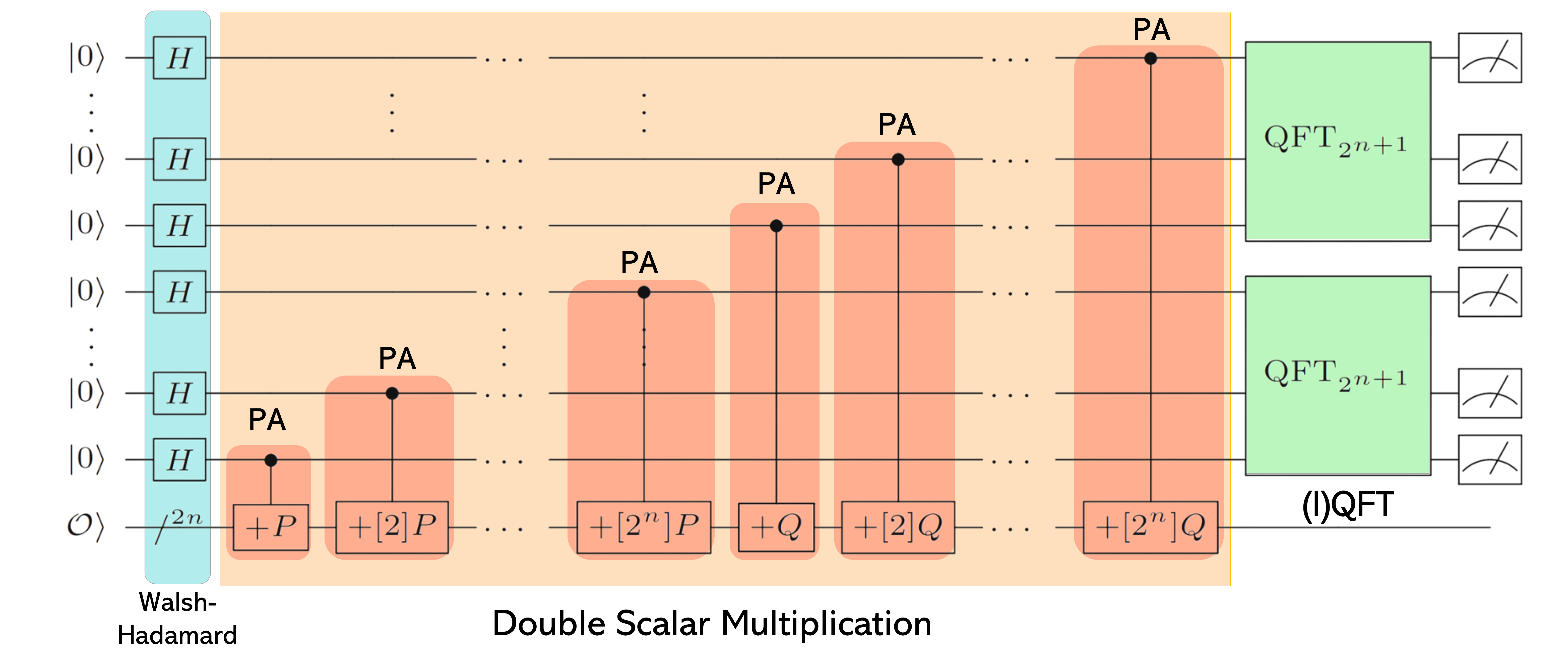
Figure 1: Quantum circuit of Shor’s algorithm for solving the elliptic curve discrete logarithm problem (ECDLP). Figures adapted from [roetteler2017quantum, larasati2023depth].

2.1 Shor’s ECDLP

The security of elliptic curve cryptography (ECC) is based on the hardness of the elliptic curve discrete logarithm problem (ECDLP). In this problem, given two points $P$ and $Q$ on an elliptic curve of order $r$, it is easy to compute the point multiplication $Q=kP$ when the scalar $k$ and the base point $P$ are known. In contrast, the reverse problem of finding the scalar $k$ given both points $P$ and $Q$ is computationally intensive [roetteler2017quantum] and considered classically intractable.

How it works. Shor’s algorithm for solving elliptic curve discrete logarithm problems (Shor’s ECDLP) works by essentially running a brute-force attack of computing the scalar multiplication of all states, but intelligently utilizing quantum interference to boost the likelihood of obtaining the desired result while suppressing the undesired value via quantum Fourier transform (QFT). As illustrated in Fig. 1, the algorithm consists of three registers with two $n+1$-sized quantum registers initialized in the state $\ket{0}$ appended with the Walsh-Hadamard (i.e., Hadamard gate on each qubit), which yields the state $\frac{1}{2^{n+1}}\sum_{k,l=0}^{2^{n+1}-1}{{k,l}}$. Subsequently, conditional to the state of the register containing $k$ or $l$, the corresponding multiple of points $P$ and $Q$ are added via the double-scalar multiplication circuit, performing the mapping as in Eq. 1 [roetteler2017quantum],

$$\frac{1}{2^{n+1}}\sum_{k,l=0}^{2^{n+1}-1}{{k,l}}\mapsto\sum_{k,l=0}^{2^{n+1}-1}{{k,l}}\ket{\left[k\right]P+\left[l\right]Q}$$ (1)

before appending QFT and measuring the result. Finally, classical post-processing is performed, which theoretically can yield the sought value with high probability. Consequently, this algorithm enables an adversary with a large-scale, full-fledged quantum computer to obtain $k$ by running the algorithm a few times.

Quantum scalar multiplication circuit. In existing works, as previously shown in Fig. 1, the quantum (double) scalar multiplication circuit comprises solely of (controlled) point addition operation, simplifying the operation by making the added point fixed. However, this does not cover the case where both points are the same, which necessitate the use of point doubling operation, therefore may yield incorrect result when doubling the points [proos2003shor]. Even though it is argued that the fidelity loss from this is small, the stricter case will require the analysis of the point-doubling circuit as well. Therefore, it is beneficial to analyze the point doubling circuit, which we start with this paper.

2.2 Binary Elliptic Curves in the Quantum Realm

From a quantum cryptanalysis perspective, an ordinary binary elliptic curve is often considered instead of other stronger variants such as supersingular [banegas2021concrete]. Here, we first describe the theoretical concept of binary elliptic curves. The Weierstrass equation for an ordinary binary elliptic curve is described in Eq. 2,

$$y^{2}+xy=x^{3}+ax^{2}+b$$ (2)

where $a\in\mathbb{F}_{2}$ and $b\in\mathbb{F^{*}}_{2^{m}}$ (i.e., the extension field). Then, the points on this elliptic curve, $P=(x,y)\in\mathbb{F^{2}}_{2^{m}}$, form a set of points that can be computed under the elliptic curve group law comprising point addition and point doubling operations. In particular, point addition, e.g., $P_{1}+P_{2}=P_{3}$, with $P_{1}=(x_{1},y_{1})$, $P_{2}=(x_{2},y_{2})\neq\pm P_{1}$, and $P_{3}=(x_{3},y_{3})$, can be computed by following Eqs. 3 to 5.

$$x_{3} =\lambda^{2}+\lambda+x_{1}+x_{2}+a$$ (3)

$$y_{3} =\lambda(x_{1}+x_{3})+x_{3}+y_{1}$$ (4)

$$\lambda =\frac{y_{1}+y_{2}}{x_{1}+x_{2}}$$ (5)

Meanwhile, the point doubling calculation is as shown in Eqs. 6 to 8. [hankerson2006guide, pornin2022efficient].

$$x_{3} =\lambda^{2}+\lambda+a={x_{1}}^{2}+\frac{b}{{x_{1}}^{2}}$$ (6)

$$y_{3} ={x_{1}}^{2}+(\lambda+1)x_{3}$$ (7)

$$\lambda =x_{1}+y_{1}/x_{1}$$ (8)

Constructing the quantum circuit. From the group law formula above, the corresponding quantum circuit can be constructed. Regarding the quantum point addition circuit, the recent concrete construction is by Banegas et al. [banegas2021concrete], which is presented in Fig. 2. As inferred from the figure, the circuit requires three registers of size $n$ in which two serve as input/output registers and one as a clean ancilla register, plus one qubit serving as the control —which in the full scheme of Shor’s ECDLP circuit will be associated with the qubit in the upper registers (the ones appended by Walsh-Hadamard). Additionally, the circuit utilizes two multiplications, two divisions, and two squarings —all of which are conditionally controlled, linked to the control qubit and other associated register —and several (controlled) additions and addition by a constant.

Quantum resource cost. In terms of the exact resource count, however, it will greatly depend on the underlying subroutines employed since the aforementioned circuit is still a high-level architecture that will be broken down into its finer-grained components. For instance, choosing to use between two different inversion techniques: greatest common divisor (GCD) [banegas2021concrete] or Fermat’s Little Theorem (FLT) [banegas2021concrete, larasati2023depth, taguchi2023concrete] for the division subroutines, or between Schoolbook [vedral1996quantum] and Karatsuba multiplication [vanhoof2019space, putranto2023depth, gidney2019asymptotically, jang2022optimized] will yield quite different performance metrics, including in terms of the total number of qubits (i.e., qubit count or circuit width), circuit depth (i.e., the longest path for the quantum operations to run on the quantum hardware, gate count (i.e., the total number of quantum gates), as well as the more specific terms like Toffoli depth and Toffoli count [gyongyosi2020circuit, ucberkeley_2007].

@C=1em @R=.7em &|x_1⟩ /^n +x_2 2 2 +a +x_2 2 2 +x_2 1 |x_3⟩ or |x_1⟩
|q⟩ 1 -1 -1 -1 1 1 |q⟩
|y_1⟩ /^n +y_2 1 M S -1 S M 1 +y_2 |y_3⟩ or |y_1⟩
|0⟩ /^n D -1 -1 -2 -1 -1 D |0⟩

Figure 2: Point addition circuit for binary elliptic curves proposed by Banegas et al [banegas2021concrete].

3 Quantum Circuit Designs of Point Doubling Operation for Binary Elliptic Curves

In this section, we start by elaborating on the challenges in constructing point-doubling operations. Furthermore, we provide three circuits for point doubling to suit different design considerations. In this work, we aim to be clear also for non-expert audiences; therefore, we describe our thought process to develop the resulting circuit.

3.1 Challenges on Quantum Point Doubling Construction

Before going into detail about the point-doubling circuit itself, it would be better to start with the differences between point addition and point doubling from the quantum perspective that we are able to identify. Constructing a point-doubling circuit poses relatively more difficulties than a point-addition circuit. Firstly, to implement point addition, previous works [proos2003shor] proposed simplification by making one of the two points constant, which is added conditionally depending on the state of the control qubit (which represents each qubit that is appended by Hadamard gates in the upper registers of Shor’s ECDLP, see Fig. 1).

With this, the point to be added (i.e., $P_{2}(x_{2},y_{2})$) is appended conditionally as a constant; hence can be pre-set and precomputed classically. Furthermore, by making the point a constant, the uncomputation process can be performed with ease since the added point can be immediately subtracted or uncomputed as soon as they are no longer needed in the calculation, making it practical and more efficient. Secondly, as mentioned in [proos2003shor] and further elaborated in [roetteler2017quantum], by looking further at the point addition formulas (Eqs. 3 to 5), the value of $\lambda$ in point addition has a direct, clear relation with both $x_{1}$ and $x_{3}$, as well as $y_{1}$ and $y_{3}$ (i.e., $x_{3}$ can be obtained from appending $x_{2}$ and $\lambda$ to $x_{1}$ with other relevant operations (Eq. 3), and similarly, $y_{3}$ can be obtained from appending $y_{1}$ and $\lambda$ to $y_{1}$ with other relevant operations (Eq. 4)). Here, we say that the initial state of $x_{1}$ and $y_{1}$ can be "consumed" to obtain the final desired computation. Then, by intelligently arranging the circuit, we can straightforwardly transform the initial state ($x_{1},y_{1}$) to the subsequent state ($x_{3},y_{3}$). As a result, an efficient computation (and uncomputation) can be achieved, and a clear reversibility relationship can be maintained.

On the other hand, the construction of point doubling is relatively tricky. First, we will discuss point doubling in a broader view without restricting ourselves to the case of Shor’s algorithm requirement. In the case of point doubling, both points involved in the computation share identical values ($P=R$). Unlike point addition, where it is reasonable to assume that the second point is constant and its value is known in advance, the same assumption does not hold for point doubling. Intuitively, if the point to be doubled were known beforehand, then the whole point doubling operation would serve no purpose.

Hence, the practice of appending the value of the second point, as seen in point addition, is not applicable in this scenario. Consequently, an extra placeholder (register) will be required to store or append the same point, which can be achieved through a "fan-out" or "copy" operation using CNOT gates. Moreover, due to both input points being quantum and the operations being conditionally dependent on the state of a controlled qubit $q$, many of the operations will ultimately require "elevation,": CNOT becomes CCNOT (controlled-controlled NOT gate a.k.a. Toffoli gate), CCNOT becomes CCCNOT (multi-controlled Toffoli gate), and so on, leading to more complex operations.

Furthermore, examining the point doubling formula in Eqs. 6 to 8, obtaining $x_{3}$ from $x_{1}$ and $y_{3}$ from $y_{1}$, is not as straightforward. The term $x_{1}$ does not directly evolve into $x_{3}$, and similarly for $y_{1}$ and $y_{3}$. In detail, as inferred from Eq. 6, obtaining $x_{3}$ from $x_{1}$ requires "copying" $x_{1}$ to be squared and then appended (i.e., $x_{1}^{2}+\frac{b}{x_{1}^{2}})$, while obtaining it from $\lambda$ does not require any $x_{1}$. Hence, we say that it does not "consume" the initial state. Similarly for $y_{3}$ as obtaining it does not make use of $y_{1}$ at all. As a consequence, the initial value of $y_{1}$ may need to be preserved in the circuit as it can not be erased, hence requiring a placeholder (such as an ancilla register) to hold its value. This makes it challenging to devise an efficient design for its quantum circuit implementation.

3.2 Proposed Quantum Circuits

Despite the challenges, there are still opportunities from the point-doubling formula that we can leverage to implement the circuit rather efficiently. We observe that there exists an indirect relation that can be taken advantage of. In particular, notice that $x_{1}$ has a direct relation to $y_{3}$, while $y_{1}$ has a direct relation to $x_{3}$. By utilizing this correlation, it is possible to transform $x_{1}$ and $y_{1}$ into $y_{3}$ and $x_{3}$, respectively. Thereby, a relatively efficient circuit can still be obtained, albeit with a "twisted" input-output relation (i.e., where $x_{1}$ maps to $y_{3}$ and $y_{1}$ maps to $x_{3}$ instead of the aligned mapping of $x_{1}$ to $x_{3}$ and $y_{1}$ to $y_{3}$).

Fundamentally, there is no requirement for the input and the output to be aligned. However, considering the conditional nature of the computation (i.e., if the control qubit $q$ is in the state zero, the doubling does not occur and the value remains as $x_{1}$ instead of being transformed into $y_{3}$) and the circuit will be incorporated into a larger scheme of scalar multiplication, a direct alignment will be helpful for clarity of the operations, which can be done simply by appending (controlled) swap gates.

Nevertheless, as previously described, the construction of point doubling may necessitate more space (i.e., ancilla registers) than that of point addition. While the latter, as proposed by Banegas et al. [banegas2021concrete], requires one ancilla register used as a placeholder for division operation (see Fig. 2), two ancilla registers will be required for performing point doubling. Below, we provide three schemes of point-doubling circuits to suit different implementation preferences.

The proposed circuits for performing point doubling are illustrated in Fig. LABEL:fig:ecc_all_pd. These circuits consist of two $n$-sized input/output registers, a control qubit $q$, and two $n$-sized ancilla registers to store intermediate results. Additionally, the presence of multiple multi-controlled gates throughout the circuit results from the circuit’s conditional nature, wherein it remains in the initial state (i.e., $x_{1}$ and $y_{1}$) when the control qubit is in the state $\ket{0}$. It is important to highlight that our proposal focuses on the high-level structure of the circuit arrangement, whereas the underlying field operations and subroutines (e.g., multiplication, squaring) may employ existing techniques such as Schoolbook or Karatsuba multiplication as proposed in [banegas2021concrete, putranto2023depth, jang2022optimized], with necessary adjustments made to accommodate the number of qubits required on each construction. The state change corresponding to these circuits is presented in Table LABEL:tab:pd_statechange. In detail, the complete steps (up to line 15) are for the third scenario (Fig. LABEL:fig:ecc_pd_full), while the second scenario (Fig. 3(b)) and the first scenario (Fig. 3(a)) terminate at lines 10 and 12, respectively.

@C=1em @R=.7em & |q⟩ 1 2 2 2 1 1 1 |q⟩
|x_1⟩ /^n 1 1 2 S |x_3⟩ or |x_1⟩
|y_1⟩ /^n 1 M S +a 1 1 -10 |y_3⟩ or |y_1⟩
|0⟩ /^n D -1 -1 -1 +1 1 1 |λ+ 1⟩
|0⟩ /^n M -3 M |0⟩

(a) Proposed point doubling circuit, with clearing one ancilla register

@C=1em @R=.7em & |q⟩ 1 2 2 2 1 1 1 |q⟩
|x_1⟩ /^n 1 1 2 S |x_3⟩ or |x_1⟩
|y_1⟩ /^n 1 M S +a 1 -10 |y_3⟩ or |y_1⟩
|0⟩ /^n D -1 -1 -1 +1 1 |λ+1⟩
|0⟩ /^n M -3 |(λ+1)x_3⟩ or
|(λ+1)y_1⟩

(b) Alternative 1: Without uncomputation

@C=1em @R=.7em & |q⟩ 1 2 2 2 1 1 1 1 1 |q⟩
|x_1⟩ /^n 1 1 2 S 2 1 |x_3⟩ or