Interactions of the $\chi_{c1}(4274)$ state with light mesons

Abstract

We investigate the interactions of the $\chi_{c1}(4274)$ state with light mesons in the hot hadron gas formed in heavy ion collisions. The vacuum and thermally-averaged cross sections of production of $\chi_{c1}(4274)$ accompanied by light pseudoscalar and light vector mesons as well as the corresponding inverse processes are estimated within the context of an effective Lagrangian approach. The results suggest non-negligible thermal cross-sections, with larger magnitudes for most of the suppression reactions than those for production. This might be a relevant feature to be considered in the analysis of future data collected in heavy ion collisions.

I Introduction

Recently, the LHCb Collaboration reported the observation of a charmoniumlike state named $\chi_{c1}(4274)$ in the amplitude analysis of the decay $B^{+}\rightarrow J/\psi\phi K^{+}$. Its quantum numbers have been established to be $I^{G}(J^{PC})=0^{+}(1^{++})$ with statistical significance of $6.0\sigma$, and its measured mass and width LHCb:2016axx ; LHCb:2016nsl

$$m=4273.3\pm 8.3^{+17.2}_{-3.6}~{}\mbox{ MeV},$$

$$\Gamma=56\pm 11^{8.0}_{-11}~{}\mbox{ MeV},$$ (1)

at $5.8\sigma$ significance. These values of mass and width are consistent with a previous measurement claimed by the CDF collaboration CDF:2011pep . Taking into account its isoscalar nature and decay mode, the $\chi_{c1}(4274)$ must have a minimum tetraquark content.

As a consequence, a great deal of effort has been made by the community in order to describe its properties and intrinsic quark configuration. We remark some examples of proposals for the interpretation of the $\chi_{c1}(4274)$. Refs. Chen:2016oma ; Wang:2016dcb considered it as a $s-$wave $cs\bar{s}\bar{c}$ tetraquark state within the framework of QCD sum rules, and  Stancu:2009ka ; Zhu:2016arf using the compact tetraquark model. Interestingly, Ref. Lu:2016cwr showed that the relativized quark model proposed by Godfrey and Isgur cannot account for the compact tetraquark configuration, but for the conventional $\chi_{c1}(3^{3}P_{1})$ state. On the other hand, the excited charmonium state configuration cannot be accommodated in the context of the ${}^{3}P_{0}$ model, as suggested by Ref. Gui:2018rvv .

The color triplet and sextet diquark-antidiquark configuration was also employed by Agaev:2017foq . Contrasting with experimental results, Ref. Maiani:2016wlq proposed that the $\chi_{c1}(4274)$ would correspond rather to two, almost degenerate, unresolved lines with $J^{PC}=0^{++},2^{++}$.

From another interesting perspective, an analysis of the $\chi_{c1}(4274)$ as a $p-$wave bound state of $D_{s}D_{s0}(2317)$ was performed in a quasipotential Bethe-Salpeter equation approach, with a partial wave decomposition on spin parity He . This comes from the fact that the $\chi_{c1}(4274)$ mass is just 12 MeV below the $D_{s}\bar{D}_{s0}(2317)$ threshold. And since the quantum numbers of $D_{s}$ and $\bar{D}_{s0}$ (henceforth we denote $\bar{D}_{s0}(2317)$ simply by $\bar{D}_{s0}$) are $0^{-}$ and $0^{+}$, the binding mechanism between these two mesons must be in $p-$wave and strong to form a bound state. However, via an effective approach Ref. zhu2022possible argued that the partial decay widths of the $\chi_{c1}(4274)$ do not favor the $p-$wave bound state interpretation, but indicates the possibility of a new state so-called $Y^{\prime}(4274)$, which might be found in experiments such as Belle and Belle II. In the end, the intrinsic nature and the properties of the $\chi_{c1}(4274)$ is still a matter of debate, and more experimental and theoretical studies are really needed.

We believe that heavy-ion collisions (HICs) provide a promising scenario to investigate the properties of exotic states CMS:2021znk . As discussed in precedent works, at the end of the quark-gluon plasma phase quarks coalesce to form all types of hadronic states. The exotic states are then formed and can interact with other light hadrons during the hadron gas phase ChoLee1 ; XProd1 ; XProd2 ; Abreu:2017cof ; Abreu:2018mnc ; Hong:2018mpk ; Abreu:2021jwm ; Abreu:2022lfy ; AbreuZcs . Their final multiplicities will depend on the interaction cross sections, which, in turn, depend on the spatial configuration of the quarks. Meson molecules are larger, and therefore have greater cross sections, which means that they will have a more prominent interaction with the hadronic medium than compact tetraquarks.

In this work we investigate the interactions of the $\chi_{c1}(4274)$ state with light mesons within the context of an effective Lagrangian approach. The vacuum and thermally-averaged cross sections of reactions involving the production of $\chi_{c1}(4274)$ accompanied by pseudoscalar mesons $\pi,K$ and $\eta$ and vector mesons $\rho,K^{*}$ and $\omega$ as well as the corresponding inverse processes are estimated. We would like to emphasize that:

i) The hadron gas formed in heavy ion collisions lives for $\simeq 10$ fm and the time scale of strong interactions is $\simeq 1$ fm. Therefore the multiquark states (tetraquarks or molecules) will inevitably interact with the light hadrons of the medium.

ii) The careful study of the ratio $\chi_{c1}(3872)/\psi(2S)$ as a function of the system size published in rat-dat made even more clear that the final state interactions (i.e., interactions within the hadron gas) are crucial to understand the data xing giving extra support to the statement i).

iii) Simplifying assumptions concerning these interactions such as the use of constant matrix elements or the use of geometrical arguments to estimate the cross sections are not sufficient. The collision energies are of the order of the temperature, i.e., $\simeq 100-200$ MeV. In this energy range the cross sections are still sensitive to resonance formation and other details of the interactions.

In view of these considerations, we will keep, as in previous works, trying to describe the multiquark interactions within the hadron gas with effective Lagrangians. In the next section we will briefly describe the formalism employed in this work. In section III we calculate the interaction cross sections, in section IV we present the thermally averaged cross sections (called from now on simply thermal cross sections), which are the really relevant quantities for transport model calculations. Finally, in section V we present some conclusions.

II Formalism

In this section, we will investigate the interactions of the $\chi_{c1}(4274)$ state with the lightest pseudoscalar mesons ($\pi,K$ and $\eta$) and with the lightest vector mesons ($\rho$, $\omega$ and $K^{*}$). We will study the reactions $\chi_{c1}(4274)\,+\,(\pi,K,\eta,\rho,K^{*},\omega)\to(\bar{D}_{s}D^{(*)},D_{s0}D_{s}^{(*)},D_{s0}D_{s0})$, as well as the inverse processes. The lowest-order Born diagrams that contribute to the processes of our interest are shown in Figs. 1 and 2. To calculate their respective amplitudes, we use an effective theory formalism in which the vector mesons are interpreted as dynamical gauge bosons of the hidden $U(N)_{V}$ local symmetry (see Refs. XProd1 ; XProd2 ; Abreu:2017cof ; Abreu:2018mnc for a more detailed discussion). In particular, the following effective Lagrangians involving the light and charmed mesons are employed:

$$\mathcal{L}_{PPV} = -ig_{PPV}\langle V^{\mu}[P,\partial_{\mu}P]\rangle,$$ (2)

$$\mathcal{L}_{VVP} = \frac{g_{VVP}}{\sqrt{2}}\varepsilon^{\mu\nu\alpha\beta}\langle\partial_{\mu}V_{\nu}\partial_{\alpha}V_{\beta}\rangle,$$ (3)

where $P$ and $V$ are the matrices in $\rm SU(4)$ flavor space containing the pseudoscalar and vector meson fields,

$$\raggedleft P\@add@raggedleft = \left(\begin{array}[]{cccc}\frac{\eta}{\sqrt{6}}+\frac{{\eta_{c}}}{\sqrt{12}}+\frac{{\pi^{0}}}{\sqrt{2}}&{\pi^{+}}&{K^{+}}&{\bar{D}^{0}}\\ {\pi^{-}}&\frac{\eta}{\sqrt{6}}+\frac{{\eta_{c}}}{\sqrt{12}}-\frac{{\pi^{0}}}{\sqrt{2}}&{K^{0}}&{D^{-}}\\ {K^{-}}&{\bar{K}^{0}}&\frac{{\eta_{c}}}{\sqrt{12}}-\frac{2\eta}{\sqrt{6}}&{D_{s}^{-}}\\ {D^{0}}&{D^{+}}&{D_{s}^{+}}&{\eta_{c}}\\ \end{array}\right),$$ (8)

$$V = \left(\begin{array}[]{cccc}\frac{\rho^{0}}{\sqrt{2}}+\frac{{\omega}}{\sqrt{6}}+\frac{J/\psi}{\sqrt{12}}&{{\rho^{+}}}&{{K^{*+}}}&{{\bar{D}^{*0}}}\\ {{\rho^{-}}}&-\frac{\rho^{0}}{\sqrt{2}}+\frac{{\omega}}{\sqrt{6}}+\frac{J/\psi}{\sqrt{12}}&{{K^{*0}}}&{{D^{*-}}}\\ {{K^{*-}}}&{{\bar{K}^{*0}}}&-2\frac{{\omega}}{\sqrt{6}}+\frac{J/\psi}{\sqrt{12}}&{{D_{s}^{*-}}}\\ {{D^{*0}}}&{{D^{*+}}}&{{D_{s}^{*+}}}&-3\frac{J/\psi}{\sqrt{12}}\\ \end{array}\right);$$ (13)

the coupling constants are given by:

$$g_{PPV} = \frac{m_{V}}{2f_{\pi}}\frac{m_{D^{*}}}{m_{K^{*}}},$$

$$g_{VVP} = \frac{3m^{2}_{V}}{16\pi^{2}f^{3}_{\pi}},$$ (14)

with $m_{V}$ being the mass of the vector meson; we take it as the mass of the $\rho$ meson and $f_{\pi}$ is the pion decay constant. As pointed in Ref. XProd1 , the factor $m_{D^{*}}/m_{K^{*}}$ in the coupling $g_{PPV}$ is introduced in order to reproduce the experimental decay width found for the process $D^{*}\to D\pi$, and comes from heavy-quark symmetry considerations.

Figure 1: Born diagrams describing the production of the $\chi_{c1}(4274)$ (denoted by $\chi_{c1}$) and a light pseudoscalar meson (without specification of the charges of the particles).

Figure 2: Born diagrams describing the production of the $\chi_{c1}(4274)$ (denoted by $\chi_{c1}$) and a light vector meson (without specification of the charges of the particles).

Let us now introduce the vertex associated to the $\chi_{c1}(4274)$ state. The quantum numbers of $\chi_{c1}(4274)$ are $I(J^{PC})=0(1^{++})$ and those of $D_{s}$ and $D_{s0}$ are $J^{P}=0^{-}$ and $J^{P}=0^{+}$ respectively. Hence, for parity reasons, the vertex $\chi_{c1}\,D_{s}\,D_{s0}$ must be in relative $P$-wave. This can be implemented by a term with a derivative coupling in the Lagrangian. The appropriate effective Lagrangian is then given by  zhu2022possible :

$$\mathcal{L}_{\chi_{c1}}=\frac{1}{\sqrt{2}}g_{\chi_{c1}D_{s}\bar{D}_{s0}}\chi_{c1}^{\mu}\left[D^{+}_{s}\overset{\leftrightarrow}{\partial}_{\mu}D^{-}_{s0}-D^{-}_{s}\overset{\leftrightarrow}{\partial}_{\mu}D^{+}_{s0}\right],$$ (15)

where $\chi_{c1}^{\mu}$ stands for the field associated to $\chi_{c1}(4274)$ state; $g_{\chi_{c1}D_{s}\bar{D}_{s0}}$ is the effective coupling constant taken from the analysis of the $\chi_{c1}(4274)$ width performed in Ref. zhu2022possible : $g_{\chi_{c1}D_{s}\bar{D}_{s0}}=13.34^{+1.11}_{-0.89}$.

Other couplings involving the $D_{s0}$ state, charmed mesons and light mesons present in the processes depicted in Figs. 1 and 2 are also needed. In the case of the light pseudoscalar mesons (in Fig. 1), the relevant three-body Lagrangians are zhu2022possible (we have used the same notation as in this reference)

$$\mathcal{L}_{KDD_{s0}} =g_{KDD_{s0}}KDD_{s0},$$

$$\mathcal{L}_{\pi^{0}D_{s}D_{s0}} =g_{\pi^{0}D_{s}D_{s0}}\pi^{0}D_{s}D_{s0},$$

$$\mathcal{L}_{\eta D_{s}D_{s0}} =g_{\eta D_{s}D_{s0}}\eta D_{s}D_{s0},$$ (16)

where the coupling constants take the values $g_{KDD_{s0}}=10.21\mbox{ GeV}$, $g_{\pi^{0}D_{s}D_{s0}}=1.3124\mbox{ GeV}$ and $g_{\eta D_{s}D_{s0}}=6.40\mbox{ GeV}$. For the three-body vertices involving the $D_{s0}$ state, charmed mesons and light vector mesons (in Fig. 2), we employ the following Lagrangians  VMD

$$\mathcal{L}_{VD_{s0}D_{s0}} =-ig_{VD_{s0}D_{s0}}V^{\mu}D_{s0}^{-}\overset{\leftrightarrow}{\partial}_{\mu}D_{s0}^{+},$$

$$\mathcal{L}_{VD_{s0}D_{s}^{*}} =g_{VD_{s0}D_{s}^{*}}[D_{s0}^{-}D_{s\mu\nu}^{*+}-D_{s0}^{+}D_{s\mu\nu}^{*-}]V_{\mu\nu},$$ (17)

where $V_{\mu\nu}=\partial_{\mu}V_{\nu}-\partial_{\nu}V_{\mu}$. The coupling constants $g_{VD_{s0}D_{s0}}$ and $g_{VD_{s0}D_{s}^{*}}$ are estimated through the vector dominance (VMD) model VMD . Accordingly, the virtual photon in the $D_{s0}^{+}e^{-}\rightarrow D_{s0}^{+}e^{-}$ scattering is coupled to the vector meson via the photon-vector-meson mixing term

$$\gamma_{V}V^{\mu}A_{\mu},$$ (18)

where $A_{\mu}$ is the photon field; $\gamma_{V}$ is the photon-vector-meson mixing amplitude, determined from the width of the vector-to-electron-positron decay,

$$\Gamma_{V}=\frac{\alpha_{em}\gamma_{V}}{3m_{V}^{3}},$$ (19)

where $\alpha_{em}$ is the electromagnetic fine-structure constant and $m_{V}$ is the vector mass. For the $\omega$ and $\rho$ mesons we have $\Gamma_{\omega}=0.6\mbox{ keV}$ and $\Gamma_{\rho}=6.96\mbox{ keV}$ respectively PDG , which yields the mixing amplitudes $\gamma_{\omega}=0.011\mbox{ GeV}^{2}$ and $\gamma_{\rho}=0.037\mbox{ GeV}^{2}$. Next, the coupling constants $g_{\omega D_{s0}D_{s0}}$ and $g_{\rho^{0}D_{s0}D_{s0}}$ can be estimated with the following expression:

$$\frac{\gamma_{V}g_{VD_{s0}D_{s0}}}{m_{V}^{2}}=\frac{1}{3}e;$$ (20)

which gives $g_{\omega D_{s0}D_{s0}}=5.50$ and $g_{\rho^{0}D_{s0}D_{s0}}=1.66$. To obtain $g_{VD_{s0}D_{s}^{*}}$, we make use of an extension of Eq. (20), i.e.

$$\frac{\gamma_{V}g_{VD_{s0}D_{s}^{*}}}{m_{V}^{2}}=\frac{1}{3}eg_{\gamma D_{s0}D_{s}^{*}},$$ (21)

where $g_{\gamma D_{s0}D_{s}^{*}}$ is the coupling constant of the vertex involving the photon, $D_{s0}$ and $D^{*}_{s}$, which from theoretical estimates is $g_{\gamma D_{s0}D^{*}_{s}}\geq 3.02\times 10^{-2}\mbox{ GeV}$ VMD ; Faessler:2007gv , Therefore, we can write

$$g_{VD_{s0}D_{s}^{*}}=g_{VD_{s0}D_{s0}}\times g_{\gamma D_{s0}D_{s}^{*}}.$$ (22)

Taking the smallest value of $g_{\gamma D_{s0}D_{s}^{*}}$, we obtain $g_{\omega D_{s0}D_{s}^{*}}=0.17\mbox{ GeV}$ and $g_{\rho D_{s0}D_{s}^{*}}=0.050\mbox{ GeV}$. Then, the effective model above allows us to write the amplitudes corresponding to the diagrams depicted in Figs. 1 and 2 as:

$$M_{D_{s}D_{s}\rightarrow\chi_{c1}\pi}= M^{(a)}+M^{(b)},$$

$$M_{D_{s0}D_{s0}\rightarrow\chi_{c1}\pi}= M^{(c)}+M^{(d)},$$

$$M_{D_{s}D_{s}\rightarrow\chi_{c1}\eta}= M^{(e)}+M^{(f)},$$

$$M_{D_{s0}D_{s0}\rightarrow\chi_{c1}\eta}= M^{(g)}+M^{(h)},$$

$$M_{D_{s0}D_{s}^{*}\rightarrow\chi_{c1}\eta}= M^{(i)},$$

$$M_{D_{s0}D^{*}\rightarrow\chi_{c1}K}= M^{(j)},$$

$$M_{D_{s}D\rightarrow\chi_{c1}K\rightarrow}= M^{(k)},$$

$$M_{D_{s}D_{s0}\rightarrow\chi_{c1}\rho}= M^{(l)},$$

$$M_{D_{s}D_{s}^{*}\rightarrow\chi_{c1}\rho}= M^{(m)},$$

$$M_{D_{s0}D\rightarrow\chi_{c1}K^{*}}= M^{(n)},$$

$$M_{D_{s0}D^{*}\rightarrow\chi_{c1}K^{*}}= M^{(o)},$$

$$M_{D_{s0}D_{s}\rightarrow\chi_{c1}\omega}= M^{(p)}+M^{(q)},$$

$$M_{D_{s}D_{s}^{*}\rightarrow\chi_{c1}\omega}= M^{(r)},$$

$$M_{D_{s0}D_{s}^{*}\rightarrow\chi_{c1}\omega}= M^{(s)},$$ (23)

The explicit expressions are described in the Appendix A.

III Cross Sections

We define the isospin-spin-averaged cross section in the center of mass (CM) frame for a given reaction $ab\rightarrow cd$ in Eq (23) as:

$$\sigma_{ab\rightarrow cd}=\frac{1}{64\pi^{2}s}\frac{|\vec{p}_{cd}|}{|\vec{p}_{ab}|}\frac{1}{g_{a}g_{b}}\int d\Omega\sum_{S,I}|M_{ab\rightarrow cd}|^{2},$$ (24)

where $g_{a,b}=(2I_{a,b}+1)(2S_{a,b}+1)$ is the degeneracy factor of the of the particles in initial state; $s$ is the squared center-of-mass energy; $|\vec{p}_{ab}|$ and $|\vec{p}_{cd}|$ are the moduli of the three-momenta in CM frame of the initial and final particles, respectively. The summation is performed over the spin and isospin of the initial and final states, with the latter being rewritten in terms of the particle basis with the explicit charges of the particles in the initial state, i.e.

$$\sum_{I}|M_{ab\rightarrow cd}|^{2}\rightarrow\sum_{Q_{a},Q_{b}}|M_{ab\rightarrow cd}^{(Q_{1},Q_{2})}|^{2}.$$ (25)

The cross sections of the corresponding inverse reactions are evaluated by means of the detailed balance relation,

$$g_{a}g_{b}|\vec{p}_{ab}|^{2}\sigma_{ab\rightarrow cd}=g_{c}g_{d}|\vec{p}_{cd}|^{2}\sigma_{cd\rightarrow ab}.$$ (26)

Furthermore, to take into account the finite size of the hadrons and to suppress the artificial growth of the cross sections at large momenta, we make use of a monopole-like form factor,

$$F(\vec{q})=\frac{\Lambda^{2}}{\Lambda^{2}+\vec{q}^{2}},$$ (27)

where $\vec{q}$ is the transferred three-momentum in $t(u)$ channel, and $\Lambda$ is the cutoff, which we choose to be $\Lambda=2.0$ GeV. This type of form factor has been extensively employed in literature, and a detailed discussion on its role is found in Ref. Abreu:2021jwm .

The calculations are done with the isospin-averaged masses reported in the PDG PDG . Besides, to take into account the uncertainties in the coupling constant $g_{\chi_{c1}D_{s}D_{s0}}$, the results are presented in terms of bands associated to the smallest and largest possible values of $g_{\chi_{c1}D_{s}D_{s0}}$.

The cross sections for the processes discussed in previous section are plotted in Figs. 3 and 4 as functions of the CM energy $\sqrt{s}$, as well as those for the corresponding inverse reactions. In the case of $\chi_{c1}(4274)$ production, all cross sections are endothermic, showing a fast growth in the region very close to the threshold, with exception of the channel $D_{s0}D_{s0}\to\chi_{c1}\pi$. Considering the region up to $400\mbox{ MeV}$ above the corresponding thresholds, the different channels present a wide range of magnitudes $(\sim 10^{-6}-10^{0}\mbox{ mb}$. In particular, for the $\chi_{c1}(4274)$ production accompanied by pion and $\eta$ mesons, the channel with initial state $D_{s}^{0}\bar{D}_{s}^{0}$ yields the dominant contributions, while the other cases are at least one order of magnitude smaller. We also remark that the channels involving the kaon or $K^{*}$ mesons give contributions of similar order. Besides, the reactions involving the $\rho^{0}$ mesons with the initial or final state $D_{s}\bar{D}_{s}^{*}$ present the smallest cross sections due to the smaller coupling constant of the $\rho D_{s0}D_{s}^{*}$ interaction.

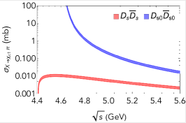
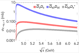
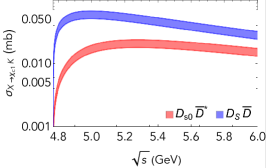
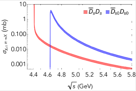
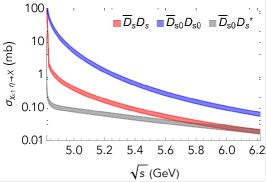
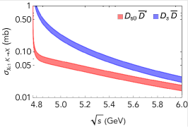
Figure 3: Top: cross sections for the production processes $\chi_{c1}(4274)\pi$ (left), $\chi_{c1}(4274)\eta$ (center) and $\chi_{c1}(4274)K$ (right), as functions of $\sqrt{s}$. Bottom: cross sections for the corresponding inverse reactions.

Let us now look at the $\chi_{c1}(4274)$-suppression processes in Figs. 3 and 4. As expected only the process $\chi_{c1}\pi\rightarrow D_{s0}D_{s0}$ is endothermic; the other absorption cross sections are exothermic, becoming very large at the threshold. Above the threshold, these cross sections have very distinct magnitudes. Most importantly, when we compare $\chi_{c1}(4274)$ absorption and production by comoving light mesons in the relevant region of energies for heavy ion collisions ($\sqrt{s}-\sqrt{s_{0}}<\,0.6$ GeV), in general the absorption cross sections are greater than the production ones. This feature reflects the differences of these reactions concerning the phase space as well the degeneracy factors encoded in Eq. (26).

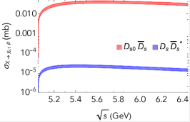
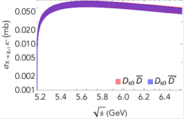
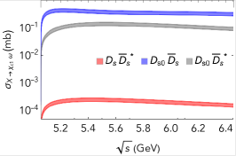
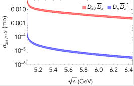
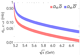
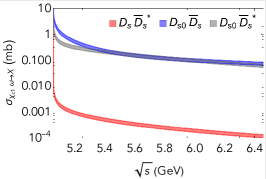
Figure 4: Top: cross sections for the production processes $\chi_{c1}(4274)\rho$ (left), $\chi_{c1}(4274)K^{*}$ (center) and $\chi_{c1}(4274)\omega$ (right), as functions of $\sqrt{s}$. Bottom: cross sections for the corresponding inverse reactions. In the process $X\rightarrow\chi_{c1}K^{*}$ the curves are slightly overlapped.

IV Thermal cross sections

The findings of the previous sections allow us to go ahead and use them as input in the analysis of the $\chi_{c1}(4274)$ production and suppression in a heavy ion collision environment, in which the medium effects become relevant. The collision energy is related to the temperature of the hadronic medium, and hence we need to evaluate the thermally averaged cross-sections, which are defined as the cross-sections averaged over the thermal distributions of the particles participating in the reactions. For the process $ab\rightarrow cd$ they are given by the convolution of vacuum cross-sections and the momentum distributions:

$$\left\langle\sigma_{ab\rightarrow cd}v_{ab}\right\rangle= \frac{\int d^{3}\mathbf{p}_{a}d^{3}\mathbf{p}_{b}f_{a}\left(\mathbf{p}_{a}\right)f_{b}\left(\mathbf{p}_{b}\right)\sigma_{ab\rightarrow cd}v_{ab}}{\int d^{3}\mathbf{p}_{a}d^{3}\mathbf{p}_{b}f_{a}\left(\mathbf{p}_{a}\right)f_{b}\left(\mathbf{p}_{b}\right)}$$

$$= \frac{1}{4\beta_{a}^{2}K_{2}\left(\beta_{a}\right)\beta_{b}^{2}K_{2}\left(\beta_{b}\right)}$$

$$\times\int_{z_{0}}^{\infty}dzK_{1}(z)\sigma\left(s=z^{2}T^{2}\right)$$

$$\times\left[z^{2}-\left(\beta_{a}+\beta_{b}\right)^{2}\right]\left[z^{2}-\left(\beta_{a}-\beta_{b}\right)^{2}\right],$$ (28)

where $f(p)$ is the Bose-Einstein distribution, $v_{ab}$ is the relative velocity of the two initial particles $a$ and $b$; $\beta_{i}=m_{i}/T$, where $T$ is the temperature; $z_{0}=max(\beta_{a}+\beta_{b},\beta_{c}+\beta_{d})$, and $K_{1}$ and $K_{2}$ are the modified Bessel functions of second kind. In Figs. 5 and 6 we plot the thermal cross section as functions of temperature. The suppression processes have a weaker dependence with the temperature than those for $\chi_{c1}(4274)$ production.

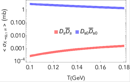
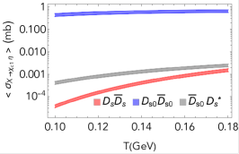
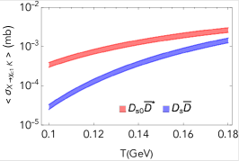
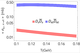
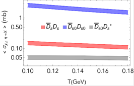
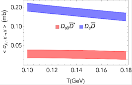
Figure 5: Top: thermal cross sections for the production processes $\chi_{c1}(4274)\pi$ (left), $\chi_{c1}(4274)\eta$ (center) and $\chi_{c1}(4274)K$ (right), as functions of temperature. Bottom: cross sections for the corresponding inverse reactions.

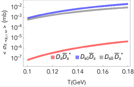
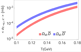
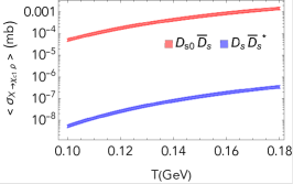
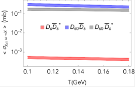
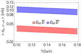
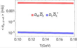
Figure 6: Top: thermal cross sections for the production processes $\chi_{c1}(4274)\rho$ (left), $\chi_{c1}(4274)K^{*}$ (center) and $\chi_{c1}(4274)\omega$ (right), as functions of temperature. Bottom: cross sections for the corresponding inverse reactions.

Comparing all the cross sections shown in the figures, the striking conclusion is that (unlike the case of most of the other exotic states) the most important process is $\chi_{c1}(4274)$ production through the reaction $D_{s0}\,\bar{D}_{s0}\to\chi_{c1}(4274)\,\pi$. The dominant absorption reaction is $\chi_{c1}(4274)\,\eta\to D_{s0}\,\bar{D}_{s0}$. In a hot hadron gas the abundance of $\eta$ is larger than the abundances of $D_{s0}$ and $\bar{D}_{s0}$. This may compensate the difference in the cross sections, but at this point we can not say that there will be a $\chi_{c1}(4274)$ suppression due to hadronic medium effects. To know what really happens we must solve the rate equations with the above cross sections. This will be addressed in a forthcoming publication.

V Conclusions

In this work we have studied the interactions of the $\chi_{c1}(4274)$ state with light mesons, which are the most abundant particles in the hot hadron gas formed in the late stage of heavy ion collisions. Using an effective Lagrangian approach, we computed the vacuum and thermal cross sections of $\chi_{c1}(4274)$ production (accompanied by light pseudoscalar and vector mesons) and the corresponding inverse processes. The coupling constants involving the $D_{s0}$ meson were calculated through the VMD model. The results show that the thermal cross-sections are sizeable. In almost all the cases, the absorption cross sections are larger than the production ones. However, the largest cross section is for $\chi_{c1}(4274)$ production through the reaction $D_{s0}\,\bar{D}_{s0}\to\chi_{c1}(4274)\,\pi$. Our study strongly motivates the use of the obtained cross sections as input to the rate equations, which yield the $\chi_{c1}(4274)$ multiplicity during the time evolution of a hot hadron gas. Work along this line is in progress.

Appendix A Amplitudes

The explicit expressions of the amplitudes for the processes represented in Figs. 1 are:

$$M^{(a)} = -\frac{g_{\pi^{0}D_{s}D_{s0}}g_{\chi_{c1}D_{s}\bar{D}_{s0}}}{\sqrt{2}}\epsilon^{\mu}(p_{3})(p_{3}-2p_{1})_{\mu}\frac{1}{t-m_{D_{s0}}^{2}},$$

$$M^{(b)} = \frac{g_{\pi^{0}D_{s}D_{s0}}g_{\chi_{c1}D_{s}\bar{D}_{s0}}}{\sqrt{2}}\epsilon^{\mu}(p_{3})(p_{3}-2p_{2})_{\mu}\frac{1}{u-m_{D_{s0}}^{2}},$$

$$M^{(c)} = -\frac{g_{\pi^{0}D_{s}D_{s0}}g_{\chi_{c1}D_{s}\bar{D}_{s0}}}{\sqrt{2}}\epsilon^{\mu}(p_{3})(p_{3}-2p_{1})_{\mu}\frac{1}{t-m_{D_{s}}^{2}},$$

$$M^{(d)} = \frac{g_{\pi^{0}D_{s}D_{s0}}g_{\chi_{c1}D_{s}\bar{D}_{s0}}}{\sqrt{2}}\epsilon^{\mu}(p_{3})(p_{3}-2p_{2})_{\mu}\frac{1}{u-m_{D_{s}}^{2}},$$

$$M^{(e)} = -\frac{g_{\eta D_{s}D_{s0}}g_{\chi_{c1}D_{s}\bar{D}_{s0}}}{\sqrt{2}}\epsilon^{\mu}(p_{3})(p_{3}-2p_{1})_{\mu}\frac{1}{t-m_{D_{s0}}^{2}},$$

$$M^{(f)} = \frac{g_{\eta D_{s}D_{s0}}g_{\chi_{c1}D_{s}\bar{D}_{s0}}}{\sqrt{2}}\epsilon^{\mu}(p_{3})(p_{3}-2p_{2})_{\mu}\frac{1}{u-m_{D_{s0}}^{2}},$$

$$M^{(g)} = -\frac{g_{\eta D_{s}D_{s0}}g_{\chi_{c1}D_{s}\bar{D}_{s0}}}{\sqrt{2}}\epsilon^{\mu}(p_{3})(p_{3}-2p_{1})_{\mu}\frac{1}{t-m_{D_{s}}^{2}},$$

$$M^{(h)} = \frac{g_{\eta D_{s}D_{s0}}g_{\chi_{c1}D_{s}\bar{D}_{s0}}}{\sqrt{2}}\epsilon^{\mu}(p_{3})(p_{3}-2p_{2})_{\mu}\frac{1}{u-m_{D_{s}}^{2}},$$

$$M^{(i)} = \frac{g_{PPV}g_{\chi_{c1}D_{s}\bar{D}_{s0}}}{\sqrt{3}}\epsilon^{*}_{\mu}(p_{2})\epsilon_{\nu}(p_{3})$$

$$\times(p_{2}-2p_{4})^{\mu}(p_{3}-2p_{1})^{\nu}\frac{1}{t-m_{D_{s0}}^{2}},$$

$$M^{(j)} = \frac{g_{PPV}g_{\chi_{c1}D_{s}\bar{D}_{s0}}}{\sqrt{2}}\epsilon_{\mu}^{*}(p_{2})\epsilon_{\nu}(p_{3})$$

$$\times(-p_{2}+2p_{4})^{\mu}(2p_{1}-p_{3})^{\nu}\frac{1}{t-m_{D_{s}}^{2}},$$

$$M^{(k)} = -\frac{g_{KDD_{s0}}g_{\chi_{c1}D_{s}\bar{D}_{s0}}}{2}\epsilon^{\mu}(p_{3})(-p_{3}+2p_{1})_{\mu}$$

$$\times\frac{1}{t-m_{D_{s0}}^{2}},$$

and for those depicted in Fig. 2 are

$$M^{(l)} = -\frac{g_{\chi_{c1}D_{s}\bar{D}_{s0}}g_{\rho D_{s0}{D}_{s0}}}{\sqrt{2}}\epsilon(p_{3})^{\nu}\epsilon(p_{4})^{\mu}$$

$$\times(-2p_{1}+p_{4})_{\mu}(p_{3}-2p_{2})_{\nu}\frac{1}{u-m_{D_{s0}}^{2}},$$

$$M^{(m)} = \frac{g_{\rho D_{s0}D_{s}^{*}}g_{\chi_{c1}D_{s}\bar{D}_{s0}}}{\sqrt{2}}(p_{4\mu}\epsilon_{\nu}^{*}(p_{2})-p_{4\nu}\epsilon_{\mu}^{*}(p_{2}))$$

$$\times(p^{\nu}_{2}\epsilon^{\mu}(p_{4})-p_{4}^{\mu}\epsilon^{\nu}(p_{4}))(2p_{1}-p_{3})_{\rho}\epsilon^{\rho}(p_{3})$$

$$\times\frac{1}{t-m_{D_{s0}}^{2}},$$

$$M^{(n)} = \frac{g_{PPV}g_{\chi_{c1}D_{s}\bar{D}_{s0}}}{\sqrt{2}}\epsilon^{\mu}(p_{4})\epsilon^{\nu}(p_{3})$$

$$\times(p_{4}-2p_{2})_{\mu}(2p_{1}-p_{3})_{\nu}\frac{1}{t-m_{D_{s}}^{2}},$$

$$M^{(o)} = \frac{g_{VVP}g_{\chi_{c1}D_{s}D_{s0}}}{{2}}\epsilon^{\mu\nu\alpha\beta}\varepsilon^{\rho}(p_{3})\varepsilon^{\beta}(p_{4})\varepsilon^{\nu}(p_{2})$$

$$\times(p_{4})_{\alpha}(p_{2})_{\mu}(2p_{1}-p_{3})_{\rho}\frac{1}{t-m_{D_{s}}^{2}}$$

$$M^{(p)} = -\frac{g_{PPV}g_{\chi_{c1}D_{s}\bar{D}_{s0}}}{\sqrt{3}}\epsilon(p_{3})^{\nu}\epsilon(p_{4})^{\mu}$$

$$\times(2p_{2}-p_{4})_{\mu}(2p_{1}-p_{3})_{\nu}\frac{1}{t-m_{D_{s}}^{2}}$$

$$M^{(q)} = \frac{g_{\chi_{c1}D_{s}\bar{D}_{s0}}g_{\omega D_{s0}D_{s}}}{\sqrt{2}}\epsilon(p_{3})^{\nu}\epsilon(p_{4})^{\mu}$$

$$\times(p_{4}-2p_{1})_{\mu}(p_{3}-2p_{2})_{\nu}\frac{1}{u-m_{D_{s0}}^{2}}$$

$$M^{(r)} = \frac{g_{\omega D_{s0}D_{s}^{*}}g_{\chi_{c1}D_{s}\bar{D}_{s0}}}{\sqrt{2}}(p_{4\mu}\epsilon_{\nu}^{*}(p_{2})-p_{4\nu}\epsilon_{\mu}^{*}(p_{2}))$$

$$\times(p^{\nu}_{2}\epsilon^{\mu}(p_{4})-p_{4}^{\mu}\epsilon^{\nu}(p_{4}))[(2p_{1}-p_{3})_{\rho}]\epsilon^{\rho}(p_{3})$$

$$\times\frac{1}{t-m_{D_{s0}}^{2}}$$

$$M^{(s)} = \frac{g_{VVP}g_{\chi_{c1}D_{s}\bar{D}_{s0}}}{\sqrt{6}}\epsilon^{\mu\nu\alpha\beta}\varepsilon^{\rho}(p_{3})\varepsilon^{\nu}(p_{4})\varepsilon^{*\beta}(p_{2})$$

$$\times(p_{4})_{\mu}(p_{2})_{\alpha}(-2p_{1}+p_{3})_{\rho}\frac{1}{t-m_{Ds}^{2}}$$

In these expressions $p_{1}$ and $p_{2}$ are the momenta of the initial states and $p_{3}$ and $p_{4}$ are the momenta of the final states. The $\varepsilon^{\mu}(p_{i})$ is the polarization of vector states with momenta $p_{i}$; $u$ and $t$ are the Mandelstam variables, which jointly with $s$, are defined as follows: $s=(p_{1}+p_{2})^{2}$, $u=(p_{1}-p_{4})^{2}$ and $t=(p_{1}-p_{3})^{2}$.

References

- (1) R. Aaij et al. [LHCb], Phys. Rev. Lett. 118 (2017) no.2, 022003 doi:10.1103/PhysRevLett.118.022003 [arXiv:1606.07895 [hep-ex]].
- (2) R. Aaij et al. [LHCb], Phys. Rev. D 95 (2017) no.1, 012002 doi:10.1103/PhysRevD.95.012002 [arXiv:1606.07898 [hep-ex]].
- (3) T. Aaltonen et al. [CDF], Mod. Phys. Lett. A 32 (2017) no.26, 1750139 doi:10.1142/S0217732317501395 [arXiv:1101.6058 [hep-ex]].
- (4) H. X. Chen, E. L. Cui, W. Chen, X. Liu and S. L. Zhu, Eur. Phys. J. C 77 (2017) no.3, 160 doi:10.1140/epjc/s10052-017-4737-5 [arXiv:1606.03179 [hep-ph]].
- (5) Z. G. Wang, Eur. Phys. J. C 77 (2017) no.3, 174 doi:10.1140/epjc/s10052-017-4751-7 [arXiv:1612.00195 [hep-ph]].
- (6) F. Stancu, J. Phys. G 37 (2010), 075017 [erratum: J. Phys. G 46 (2019) no.1, 019501] doi:10.1088/0954-3899/37/7/075017 [arXiv:0906.2485 [hep-ph]].
- (7) R. Zhu, Phys. Rev. D 94 (2016) no.5, 054009 doi:10.1103/PhysRevD.94.054009 [arXiv:1607.02799 [hep-ph]].
- (8) Q. F. Lü and Y. B. Dong, Phys. Rev. D 94 (2016) no.7, 074007 doi:10.1103/PhysRevD.94.074007 [arXiv:1607.05570 [hep-ph]].
- (9) L. C. Gui, L. S. Lu, Q. F. Lü, X. H. Zhong and Q. Zhao, Phys. Rev. D 98 (2018) no.1, 016010 doi:10.1103/PhysRevD.98.016010 [arXiv:1801.08791 [hep-ph]].
- (10) S. S. Agaev, K. Azizi and H. Sundu, Phys. Rev. D 95 (2017) no.11, 114003 doi:10.1103/PhysRevD.95.114003 [arXiv:1703.10323 [hep-ph]].
- (11) L. Maiani, A. D. Polosa and V. Riquer, Phys. Rev. D 94 (2016) no.5, 054026 doi:10.1103/PhysRevD.94.054026 [arXiv:1607.02405 [hep-ph]].
- (12) J. He, Phys. Rev. D 95, 074004(2017).
- (13) H. Q. Zhu and Y. Huang, Phys. Rev. D 105, 056011(2022).
- (14) A. M. Sirunyan et al. [CMS], Phys. Rev. Lett. 128,032001 (2022).
- (15) S. Cho and S. H. Lee, Phys. Rev. C 88, 054901(2013).
- (16) A. Martinez Torres, K. P. Khemchandani, F. S. Navarra, M. Nielsen and L. M. Abreu, Phys. Rev. D 90, 114023 (2014); A. Martinez Torres, K. P.Khemchandani, F. S. Navarra, M. Nielsen and L. M. Abreu, Acta Phys. Pol. B Proc. Supp. 8, 247 (2015).
- (17) L. M. Abreu, K. P. Khemchandani, A. Martinez Torres, F. S. Navarra and M. Nielsen, Phys. Lett. B 761, 303 (2016).
- (18) L. M. Abreu, K. P. Khemchandani, A. Martínez Torres, F. S. Navarra and M. Nielsen, Phys. Rev. C 97 044902 (2018).
- (19) L. M. Abreu, F. S. Navarra and M. Nielsen, Phys. Rev. C 101, 014906 (2020).
- (20) J. Hong, S. Cho, T. Song and S. H. Lee, Phys. Rev. C 98, 014913 (2018).
- (21) L. M. Abreu, F. S. Navarra, M. Nielsen and H. P. L. Vieira, Eur. Phys. J. C 82, 296 (2022).
- (22) L. M. Abreu, F. S. Navarra and H. P. L. Vieira, Phys. Rev. D 105, 116029 (2022).
- (23) L. M. Abreu, F. S. Navarra and H. P. L. Vieira, Phys. Rev D 106, 076001 (2022).
- (24) A. M. Sirunyan et al. (CMS), Phys. Rev. Lett. 128, 032001 (2022); R. Aaij et al. (LHCb), Phys. Rev. Lett. 126, 092001 (2021)
- (25) Y. Guo, X. Guo, J. Liao, E. Wang and H. Xing, [arXiv:2302.03828 [hep-ph]].
- (26) Y.-L. Ma. Phys. Rev. D, 82, 015013 (2010).
- (27) P.A. Zyla et al. (Particle Data Group), Prog. Theor. Exp. Phys. 2020, 083C01 (2020).
- (28) A. Faessler, T. Gutsche, V. E. Lyubovitskij and Y. L. Ma, Phys. Rev. D 76 (2007), 014005 doi:10.1103/PhysRevD.76.014005 [arXiv:0705.0254 [hep-ph]].